SLED: Self Logits Evolution Decoding for Improving Factuality in Large Language Models

Abstract

Large language models (LLMs) have demonstrated remarkable capabilities, but their outputs can sometimes be unreliable or factually incorrect. To address this, we introduce Self Logits Evolution Decoding (SLED), a novel decoding framework that enhances the truthfulness of LLMs without relying on external knowledge bases or requiring further fine-tuning. From an optimization perspective, our SLED framework leverages the latent knowledge embedded within the LLM by contrasting the output logits from the final layer with those from early layers. It then utilizes an approximate gradient approach to enable latent knowledge to guide the self-refinement of outputs, thereby effectively improving factual accuracy. Extensive experiments have been conducted on established benchmarks across a diverse range of model families (LLaMA 2, LLaMA 3, Gemma) and scales (from 2B to 70B), including more advanced architectural configurations such as the mixture of experts (MoE). Our evaluation spans a wide variety of tasks, including multi-choice, open-generation, and adaptations to chain-of-thought reasoning tasks. The results demonstrate that SLED consistently improves factual accuracy by up to 20% compared to existing decoding methods while maintaining natural language fluency and negligible latency overhead. Furthermore, it can be flexibly combined with other decoding methods to further enhance their performance.

1 Introduction

Large Language Models (LLMs) have achieved remarkable breakthroughs in recent years, demonstrating exceptional performance across various domains [1, 2, 35, 36, 44, 47, 48]. However, a significant challenge associated with LLMs is their tendency to hallucinate or distort the truth, resulting in outputs that are not factual [15, 17, 65]. This issue of hallucination undermines the reliability and trustworthiness of LLMs in practical applications. A popular strategy for improving the LLM factuality involves refining the decoding process [43, 53].

Figure 1: Factuality decoding overview.

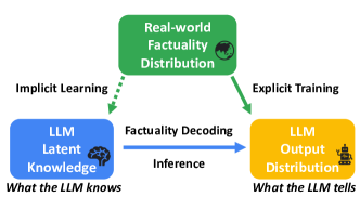
Decoding focuses on how the model selects the next token during the generation process, which can significantly influence the factual accuracy of the output. The decoding methods can be cost-effective since (a) they do not rely on external knowledge and (b) no additional training is required. Furthermore, decoding methods can be synergistically combined with other techniques aimed at improving the LLM factuality, such as retrieving information from external knowledge bases [24, 25], various fine-tuning strategies for better alignment [46, 48], or ensemble learning methods [10].

Recent studies [22, 26, 42, 50] suggest that LLMs sometimes have learned the factual content based on extensive pretraining or fine-tuning, although they fail to produce the correct answer when a user queries the model. This has inspired the development of several factuality decoding methods [7, 26, 27, 64] to reveal what the model implicitly "knows." Figure 1 summarizes the underlying mechanism of these factuality decoding methods. The LLMs’ output distribution is derived by applying the softmax function to the output logits from the final layer. During the training phase, this distribution is optimized based on the real-world factuality distribution represented by the training dataset. However, during the inference phase, "what the LLM tells" might still contain factual errors, which implies a discrepancy between the output distribution and the real-world factuality distribution. While the real-world distribution remains inaccessible during the inference phase, the model’s latent knowledge ("what the model knows") may have implicitly learned some factual content correctly during the training phase [22, 50]. Therefore, a key challenge for factuality decoding strategies lies in effectively harnessing the latent knowledge embedded within LLMs to refine the output distribution (logits) during inference.

Figure 2: Illustration of our Self Logits-Evolution Decoding (SLED) workflow.

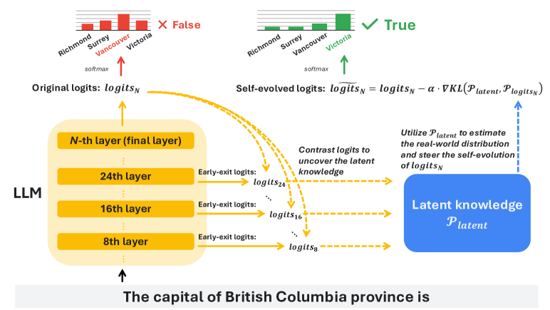
To address this challenge, we propose Self Logits Evolution Decoding (SLED), a novel factuality decoding approach that leverages the latent knowledge within LLMs by contrasting the final layer’s logits with early layers’ logits. During the decoding process, as LLMs progress from early to final layers, they progressively incorporate factual information stored in each layer into the output. SLED tracks this evolution process to unearth the latent knowledge within LLMs, and enables the “self-evolution” of the output distribution further to align it more closely with real-world facts. Furthermore, our approach recognizes that the latent knowledge within LLMs, while valuable, may not always be perfect. Therefore, instead of simply replacing the original outputs with this latent knowledge, SLED integrates it into the original logits through an operation similar to “single-step gradient descent” over the output logits during the inference time. This operation minimizes the Kullback-Leibler (KL) divergence between the latent knowledge distribution and the output distribution, effectively balancing the two and mitigating potential drawbacks such as overfitting or biased outputs. Figure 2 illustrates the SLED workflow, highlighting how SLED optimizes the output logits, leading to a more factual output distribution. We evaluate SLED on various LLMs (e.g., LLaMA 2 [48], LLaMA 3 [1], Gemma [31]) and benchmarks to demonstrate its state-of-the-art performance in layer-wise contrastive decoding methods. In summary, our main contributions are:

• We propose SLED, a novel decoding method that aligns LLMs outputs with factual knowledge without requiring an external knowledge base or fine-tuning data.

• We conduct extensive experiments across a range of LLMs, with varying configurations and scales. The results demonstrate that SLED consistently improves factual accuracy on various tasks and benchmarks, including multiple-choice, open-ended generation, and chain-of-thought reasoning tasks.

• SLED can be flexibly integrated with other factuality decoding methods to enhance their effectiveness further.

• We provide a new interpretable perspective for understanding layer-wise contrastive decoding methods, paving the way for further developments in factuality decoding.

2 Self Logits Evolution Decoding

A large language model, equipped with $\mathit{N}$ layers and a vocabulary $\mathcal{V}=[v_{1},v_{2},\ldots,v_{d}]$, typically generates text in the next-token prediction fashion. For each given prefix, the model computes the logits at the final ($\mathit{N}$-th) layer, $\mathit{logits}_{\mathit{N}}\triangleq(\ell_{(1,\mathit{N})},\ell_{(2,\mathit{N})},\ldots,\ell_{(d,\mathit{N})})$, which are obtained by applying a linear transformation to the hidden states of the final layer, projecting the high-dimensional hidden state vectors onto the space of the vocabulary size. Subsequently, the output distribution $\mathcal{P}_{\mathit{logits}_{\mathit{N}}}$ at the final ($\mathit{N}$-th) layer for the next token is derived by applying softmax function on the logits,

$$\mathcal{P}_{\mathit{logits}_{\mathit{N}}}\triangleq(p_{(1,\mathit{N})},\ldots,p_{(d,\mathit{N})})=softmax\left({\mathit{logits}_{\mathit{N}}}/{\tau}\right),$$

where $\tau$ is the temperature parameter. Therefore, for each $p_{(i,\mathit{N})}~{}(1\leq i\leq d)$, we have

$$p_{(i,\mathit{N})}={\exp(\ell_{(i,\mathit{N})}/\tau)}/{S},\ \text{where $\ S=\sum\nolimits_{j=1}^{d}\exp(\ell_{(j,\mathit{N})}/\tau).$}$$

Similarly, we can also derive the logits from early layers by applying the same linear transformation mentioned above to their hidden states. For any early layer $n~{}(n<N$), we denote its logits as $\mathit{logits}_{\mathit{n}}\triangleq(\ell_{(1,\mathit{n})},\ldots,\ell_{(d,\mathit{n})})$ and the corresponding distribution as $\mathcal{P}_{\mathit{logits}_{\mathit{n}}}\triangleq(p_{(1,\mathit{n})},\ldots,p_{(d,\mathit{n})})$.

Figure 3: We analyze the next-token predictions of three LLaMA-2-base models using the logits from each layer individually. This analysis is performed on 200 true claims from the FACTOR dataset. The results verify that the logits distribution at the final layer is closer to the real-world distribution than all the early layers in terms of KL divergence.

2.1 Logits Evolution

To improve factual accuracy, it is crucial that the correct token $v_{i}$ receives a higher value of $\mathit{logits}_{\mathit{N}}$ to ensure a higher probability value $p_{(i,\mathit{N})}$ in the output distribution $\mathcal{P}_{\mathit{logits}_{\mathit{N}}}$. From a mathematical perspective, this means aligning the model’s output distribution $\mathcal{P}_{\mathit{logits}_{\mathit{N}}}$ closely with the real-world factuality distribution $\mathcal{P}_{\mathit{real}}$. Specifically, we can formulate this goal as optimizing the following loss function $\mathcal{L}$ regarding the $\mathit{logits}$:

$$\mathcal{L}(\mathit{logits})\triangleq KL(\mathcal{P}_{\mathit{real}},\mathcal{P}_{\mathit{logits}}),\text{where}\ \mathit{logits}=(\ell_{1},...,\ell_{d}),\ \mathcal{P}_{\mathit{logits}}=softmax(\mathit{logits}/{\tau})$$ (1)

We describe the above optimization as Logits Evolution. Interestingly, the training of LLMs also aims at minimizing the divergence (typically the $\mathit{KL}$ divergence, as the training loss function is often the cross-entropy loss) between the ground truth $\mathcal{P}_{\mathit{real}}$ and the output distribution $\mathcal{P}_{\mathit{logits}_{\mathit{N}}}$. During the training phase, the logits evolution is driven externally by the real-world distribution $\mathcal{P}_{\mathit{real}}$ presented in the training dataset, and the corresponding solution is $\mathit{logits}=\mathit{logits}_{\mathit{N}}$. However, $\mathcal{P}_{\mathit{real}}$ is not accessible during the inference phase. To address this challenge, SLED utilizes the model’s latent knowledge to estimate $\mathcal{P}_{{real}}$ and enables "self-evolution" of the logits. We denote the estimation as $\mathcal{P}_{\mathit{latent}}$ and the self logits evolution can be achieved by the following gradient-descent operation:

$$\widetilde{\mathit{logits}}_{\mathit{N}}=\mathit{logits}_{\mathit{N}}-\alpha\cdot\nabla_{\mathit{logits}_{\mathit{N}}}KL(\mathcal{P}_{\mathit{latent}},\mathcal{P}_{\mathit{logits}_{\mathit{N}}}).$$ (2)

The parameter $\alpha$, termed the Evolution Rate, governs the magnitude of adjustments applied to $\mathit{logits}_{\mathit{N}}$ in the direction of the gradient $\nabla_{\mathit{logits}_{\mathit{N}}}KL(\mathcal{P}_{\mathit{latent}},\mathcal{P}_{\mathit{logits}_{\mathit{N}}})$. In the following Section 2.2 and 2.3, we discuss how we derive the $\mathcal{P}_{\mathit{latent}}$ as the estimation of the real-world distribution $\mathcal{P}_{\mathit{real}}$.

2.2 Estimate $\mathcal{P}_{\mathit{real}}$ by Tracking the Logits Evolution Direction throughout Layers

The core principle of our method involves leveraging the difference between each early layer’s logits and the final layer’s logit, $\mathit{logits}_{\mathit{n}}-\mathit{logits}_{\mathit{N}}$ to approximate the gradient of $KL(\mathcal{P}_{\mathit{real}},\mathcal{P}_{\mathit{logits}})$ at $\mathit{logits}=\mathit{logits}_{\mathit{n}}$. Then we estimate $\mathcal{P}_{\mathit{real}}$ based on this approximation.

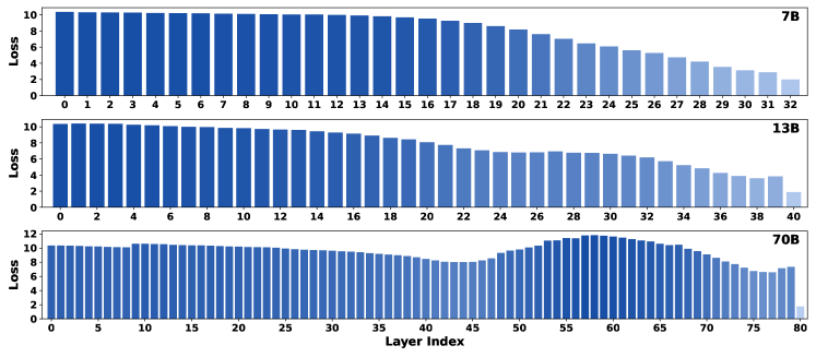
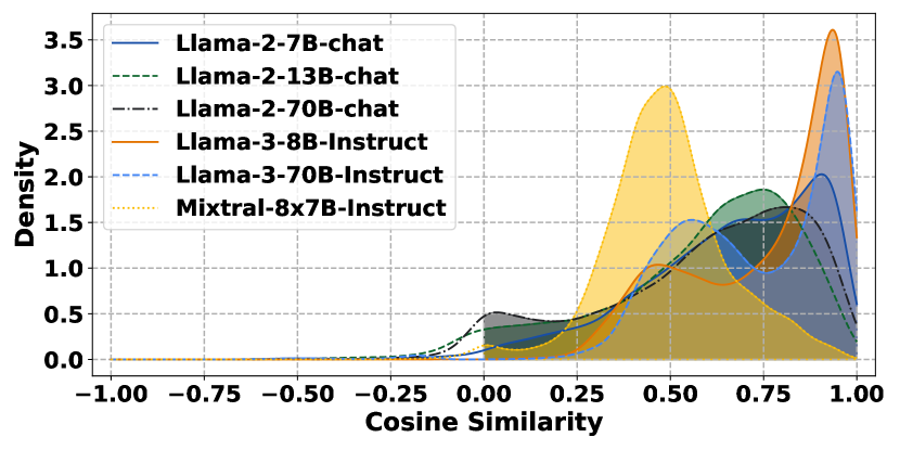
This is inspired by a new perspective of interpreting the training phase of LLMs as the evolution of logits described in Problem 1. As mentioned above, the solution derived by the training phase is the final layer’s logits $\mathit{logits}=\mathit{logits}_{\mathit{N}}$, since the final layer’s $\mathit{logits}_{\mathit{N}}$ directly engage with the real-world distribution $\mathcal{P}_{\mathit{real}}$ through the loss function in training. This implies that we can generally consider the final logits $\mathit{logits}_{\mathit{N}}$ to be a better solution than the logits from an early layer $\mathit{logits}_{\mathit{n}}$, with $KL(\mathcal{P}_{\mathit{real}},\mathcal{P}_{\mathit{logits}_{\mathit{N}}})<KL(\mathcal{P}_{\mathit{real}},\mathcal{P}_{\mathit{logits}_{\mathit{n}}})$. We present some examples in Figure 3 to demonstrate this. Based on this discussion, if we contrast the final layer’s logits with the early layer’s logits, we can consider the direction (orientation) of $\mathit{logits}_{\mathit{n}}-\mathit{logits}_{\mathit{N}}$ can approximately align with the direction of the gradient $\nabla_{\mathit{logits}}KL(\mathcal{P}_{\mathit{real}},\mathcal{P}_{\mathit{logits}})|_{\mathit{logits}=\mathit{logits}_{\mathit{n}}}$. To further verify this motivation, we calculate the cosine similarity between $\mathit{logits}_{\mathit{n}}-\mathit{logits}_{\mathit{N}}$ and $\nabla_{\mathit{logits}_{\mathit{n}}}KL(\mathcal{P}_{\mathit{real}},\mathcal{P}_{\mathit{logits}_{\mathit{n}}})$ for thousands of tokens across different models in Figure 7. We find that the majority of these values are positive, which means that the directions of these two vectors are close.

Hence, for each early layer $n$, we propose to maximize the following function of cosine similarity and derive the $\mathcal{P}^{(n)}_{\mathit{latent}}$ to estimate the $\mathcal{P}_{\mathit{real}}$.

$$\mathcal{P}^{(n)}_{\mathit{latent}}=\arg\max_{\mathcal{P}}\left(\text{CosSim}(\mathit{logits}_{\mathit{n}}-\mathit{logits}_{\mathit{N}},\nabla_{\mathit{logits}_{\mathit{n}}}KL(\mathcal{P},\mathcal{P}_{\mathit{logits}_{\mathit{n}}}),0\right)$$ (3)

2.3 Achieving the Self Logits Evolution in Three Phases

Based on the above analysis, we can introduce the procedures of SLED: First, we estimate $\mathcal{P}^{(n)}_{\mathit{latent}}$ for each early layer $n$ using the gradient approximation in Section 2.2. Subsequently, we apply a weighted average on $\{\mathcal{P}^{(n)}_{\mathit{latent}}\}$ across all early layers $n<N$ to derive $\mathcal{P}_{\mathit{latent}}$, which serves as the final estimation of the real-world distribution. Finally, we apply $\mathcal{P}_{\mathit{latent}}$ in Equation 2 to facilitate the self-evolution of ${\mathit{logits}}_{\mathit{N}}$, thereby derive the updated logits, $\widetilde{\mathit{logits}}_{\mathit{N}}$.

$${\mathit{logits}}_{\mathit{n}}-{\mathit{logits}}_{\mathit{N}} \overset{\text{in direction}}{\approx}\nabla_{\mathit{logits}_{\mathit{n}}}KL(\mathcal{P}_{\mathit{real}},\mathcal{P}_{\mathit{logits}_{\mathit{n}}})$$

$$\xRightarrow[\text{Estimate}]{{\color[rgb]{0.2578125,0.5234375,0.95703125}\definecolor[named]{pgfstrokecolor}{rgb}{0.2578125,0.5234375,0.95703125}\text{Phase 1}}}\ \mathcal{P}^{(n)}_{\mathit{latent}}\ \xRightarrow[\text{Ensemble}]{{\color[rgb]{0.2578125,0.5234375,0.95703125}\definecolor[named]{pgfstrokecolor}{rgb}{0.2578125,0.5234375,0.95703125}\text{Phase 2}}}\ \mathcal{P}_{\mathit{latent}}\ \xRightarrow[\text{Self-evolution in Eq \ref{optimized_lr_delta}}]{{\color[rgb]{0.2578125,0.5234375,0.95703125}\definecolor[named]{pgfstrokecolor}{rgb}{0.2578125,0.5234375,0.95703125}\text{Phase 3}}}\widetilde{\mathit{logits}}_{\mathit{N}}$$

Phase 1:

An exhaustive search for an exact solution to the complex optimization problem (Equation 3) is computationally impractical. We can reduce the solution space by the following. Suppose the real-world factuality distribution dictates that the next word to be generated is the $i$-th token $v_{i}$ from the vocabulary $\mathcal{V}$. Thus $\mathcal{P}_{\mathit{real}}=\mathcal{P}_{e_{i}}$, where $\mathcal{P}_{e_{i}}$ represents a standard basis vector (one-hot vector) with the $i$-th component set to 1 and all other components set to 0. Then, we can simplify the aforementioned optimization problem by limiting the solution space to $\{\mathcal{P}_{e_{i}}\}_{i=0}^{d}$ and decide which token $i$ should be selected. The corresponding gradient when $\mathcal{P}=\mathcal{P}_{e_{i}}$ has the following formulation.

Proposition 1.

The gradient of $KL(\mathcal{P}_{e_{i}},\mathcal{P}_{\mathit{logits}})$ at $\mathit{logits}=\mathit{logits}_{\mathit{n}}$ is:

$$\nabla_{\mathit{logits}_{\mathit{n}}}KL(\mathcal{P}_{e_{i}},\mathcal{P}_{\mathit{logits}_{\mathit{n}}})=(\mathcal{P}_{\mathit{logits}_{\mathit{n}}}-\mathcal{P}_{e_{i}})/{\tau}=\left(p_{(1,\mathit{n})},\ldots,p_{(i,\mathit{n})}-1,\ldots,p_{(d,\mathit{n})}\right)/{\tau}$$ (4)

We calculate the cosine similarity between the gradient $\nabla_{\mathit{logits}_{\mathit{n}}}KL(\mathcal{P}_{e_{i}},\mathcal{P}_{\mathit{logits}_{\mathit{n}}})$ and the difference $\mathit{logits}_{\mathit{n}}-\mathit{logits}_{\mathit{N}}$ for each token in the vocabulary $\mathcal{V}$. Then we select the $\mathcal{P}_{e_{i^{*}}}$ of which the gradient is closest to $\mathit{logits}_{\mathit{n}}-\mathit{logits}_{\mathit{N}}$ as the estimation $\mathcal{P}^{(n)}_{\mathit{latent}}$. Mathematically, this involves selecting $i^{*}$ according to the following criterion

$$i^{*}=\arg\max_{1\leq i\leq d}\,\bar{m}^{(n)}_{i},\ \text{where}\ \bar{m}^{(n)}_{i}=\max\left(\text{CosSim}(\mathit{logits}_{\mathit{n}}-\mathit{logits}_{\mathit{N}},\mathcal{P}_{\mathit{logits}_{\mathit{n}}}-\mathcal{P}_{e_{i}}),0\right),$$

and adopting $\mathcal{P}^{(n)}_{\mathit{latent}}=\mathcal{P}_{e_{i^{*}}}$ as the "hard estimation" of $\mathcal{P}_{\mathit{real}}$. Drawing from the concept of hard and soft targets in label smoothing and knowledge distillation, we further extend it to the "soft estimation",

$$\mathcal{P}^{(n)}_{\mathit{latent}}=(m^{(n)}_{1},\ldots,m^{(n)}_{i},\ldots,m^{(n)}_{d})/{m^{(n)}},\ \text{where}\ m^{(n)}_{i}=(\bar{m}^{(n)}_{i})^{2}\ \text{and}\ m^{(n)}={\sum\nolimits_{i=1}^{d}m^{(n)}_{i}}$$

We square $\{\bar{m}^{(n)}_{i}\}$ to moderately amplify their differences. Prior studies prove that soft targets usually offer stronger generalization capabilities, more information, and more robustness to noise than hard targets [13, 34, 45, 59, 62]. Hence, we adopt the soft estimation in lieu of the hard estimation.

Phase 2:

We ensemble $\mathcal{P}^{(n)}_{\mathit{latent}}$ across all layers by computing a weighted average of the set $\{\mathcal{P}^{(n)}_{\mathit{latent}}\}$ and adopt it as the final estimation of the $\mathcal{P}_{\mathit{latent}}$:

$$\mathcal{P}_{\mathit{latent}}={\sum\nolimits_{n=0}^{N}s^{(n)}\mathcal{P}^{(n)}_{\mathit{latent}}},\ \text{where}\ s^{(n)}=m^{(n)}/{(\sum\nolimits_{n=0}^{N}m^{(n)})}$$

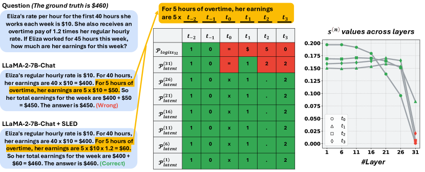
This estimation suggests that the weight $s^{(n)}$ of certain layer $n$ will be larger if the corresponding gradient approximation $\mathit{logits}_{\mathit{n}}-\mathit{logits}_{\mathit{N}}$ is more closely aligned with the gradients $\{\nabla_{\mathit{logits}_{\mathit{n}}}KL(\mathcal{P}_{e_{i}},\mathcal{P}_{\mathit{logits}_{\mathit{n}}})\}$ for the tokens in the vocabulary. This in turn amplifies the influence of layer $n$ on the final estimation, which is a desirable effect in our method. Figure 4 demonstrates that SLED can downplay incorrect tokens based on the gradient alignment. One can further validate that for each component $m_{i}$ in the final estimation $\mathcal{P}_{\mathit{latent}}\triangleq(m_{1},m_{2},\ldots,m_{d})$, the following relationship holds: $m_{i}={\sum_{n=0}^{N}m^{(n)}_{i}}/{(\sum_{n=0}^{N}\sum_{j=1}^{d}m^{(n)}_{j})}.$ This property simplifies the description in Algorithm 1.

Phase 3:

Applying $\mathcal{P}_{\mathit{latent}}$ in Equation 2 enables us to derive the gradient necessary for steering the self-evolution on the final layer’s logits $\mathit{logits}_{\mathit{N}}$.

Proposition 2.

The gradient of $KL(\mathcal{P}_{\mathit{latent}},\mathcal{P}_{\mathit{logits}})$ at $\mathit{logits}=\mathit{logits}_{\mathit{N}}$ is:

$$\nabla_{\mathit{logits}_{\mathit{N}}}KL(\mathcal{P}_{\mathit{latent}},\mathcal{P}_{\mathit{logits}_{\mathit{N}}})=(\mathcal{P}_{\mathit{logits}_{\mathit{N}}}-\mathcal{P}_{\mathit{latent}})/{\tau}=\left(p_{(1,\mathit{N})}-m_{1},\ldots,p_{(d,\mathit{N})}-m_{d}\right)/{\tau}$$

Then we can derive the self-evolved logits $\widetilde{\mathit{logits}}_{\mathit{N}}$

$$\widetilde{\mathit{logits}}_{\mathit{N}}\triangleq(\tilde{\ell}_{(1,\mathit{N})},\ldots,\tilde{\ell}_{(i,\mathit{N})},\ldots,\tilde{\ell}_{(d,\mathit{N})}),\ \text{where}\ \tilde{\ell}_{(i,\mathit{N})}={\ell}_{(i,\mathit{N})}-{\alpha}(p_{(i,\mathit{N})}-m_{i})/{\tau}.$$ (5)

Figure 4: An example from GSM8K demonstrating SLED’s mechanism. SLED derives the estimations $\mathcal{P}^{(n)}_{\mathit{latent}}$ by contrasting final layer’s logits $\mathit{logits}_{\mathit{N}}$ with early layers’ logits $\{\mathit{logits}_{\mathit{n}}\}$. We list the token with the highest probability value from the $\mathcal{P}^{(n)}_{\mathit{latent}}$ for different early layers. As shown, SLED downplays incorrect tokens by assigning lower weights $s^{(n)}$ to the corresponding $\mathcal{P}^{(n)}_{\mathit{latent}}$. Conversely, if the estimation is correct, the weights are relatively larger. The parameter evaluation scale is set to 2.

Algorithm 1 Self Logits Evolution Decoding

1:Initialization: LLM with $N$ layers, $inputs$, evolution rate $\alpha$, evolution scale $k>0$, $\eta\ll 0$, temperature parameter $\tau$, and the one-hoc vectors $\{\mathcal{P}_{e_{i}}\}$ defined in Section 2.3.

2:Feed the $inputs$ into the LLM to obtain the logits $\mathit{logits}_{\mathit{n}}=(\ell_{(1,\mathit{n})},\ldots,\ell_{(d,\mathit{n})})$ and probabilities $\mathcal{P}_{\mathit{logits}_{\mathit{n}}}=(p_{(1,\mathit{n})},\ldots,p_{(d,\mathit{n})})=softmax(\mathit{logits}_{\mathit{n}}/\tau)$ at each layer $n$, where $n\leq N$.

3:Identify the tokens with the top-$k$ largest values in $\mathit{logits}_{\mathit{N}}$ and denote their indices by $I_{k}$.

4:for each early layer $n$, $(n<N)$ do

5:     Compute differences for top-$k$ logits $\mathit{logits}_{\mathit{n}}-\mathit{logits}_{\mathit{N}}$.

6:     Calculate $m^{(n)}_{i}=\left[\max\left(\text{CosSim}(\mathit{logits}_{\mathit{n}}-\mathit{logits}_{\mathit{N}},\mathcal{P}_{\mathit{logits}_{\mathit{n}}}-\mathcal{P}_{e_{i}}),0\right)\right]^{2},i\in I_{k}$.

7:end for

8:Compute weighted average $m_{i}=\frac{\sum_{n=1}^{N}m^{(n)}_{i}}{\sum_{n=1}^{N}\sum_{j\in I_{k}}m^{(n)}_{j}}$ across different layers for each $i\in I_{k}$.

9:for each $i$ from $1$ to $d$ do

10:     Set $\tilde{\ell}_{(i,\mathit{N})}={\ell}_{(i,\mathit{N})}-\frac{\alpha}{\tau}(p_{(i,\mathit{N})}-m_{i})$ if $i\in I_{k}$ else Set $\tilde{\ell}_{(i,\mathit{N})}=\eta\ll 0$.

11:end for

12:Output: The self-evolved logits are $\widetilde{\mathit{logits}}_{\mathit{N}}=(\tilde{\ell}_{(1,\mathit{N})},\ldots,\tilde{\ell}_{(i,\mathit{N})},\ldots,\tilde{\ell}_{(d,\mathit{N})})$.

2.4 Computational Complexity and Design Decisions

For each layer, computing $\text{CosSim}(\mathit{logits}_{\mathit{n}}-\mathit{logits}_{\mathit{N}},\mathcal{P}_{\mathit{logits}_{\mathit{n}}}-\mathcal{P}_{e_{i}})$ for every token $v_{i}$ in the vocabulary $\mathcal{V}$ needs $\mathcal{O}(d^{2})$ operations. To reduce the computational complexity, we select only a subset $\mathcal{V}_{I_{k}}$, where the token $v_{i}\in\mathcal{V}_{I_{k}}$ has the top-$k$ highest logits in the final layer. In this scenario, we only initiate the self-evolution in Equation 2 of the logits corresponding to these top-$k$ tokens. For the remaining tokens, which have lower probabilities, their logits are adjusted to a very lower numerical value, e.g., $-1000$. This strategy significantly reduces the computational complexity, while maintaining focus on the most relevant tokens. We name the parameter $k$, as Evolution Scale, since it determines the number of top-probability tokens active for self-evolution.

Q 2.1: Why SLED contrast the final layer with all the early layers, instead of picking one premature layer to contrast based on JSD?

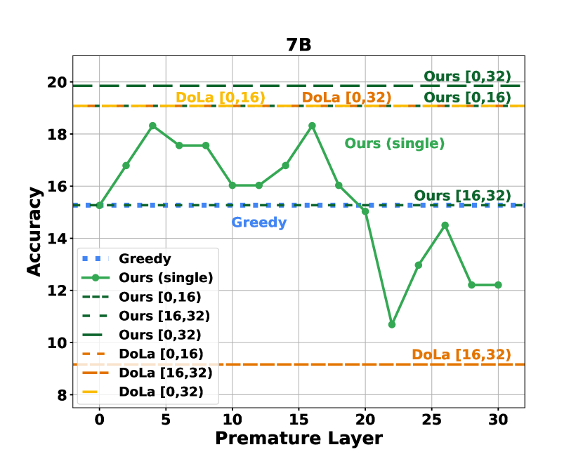
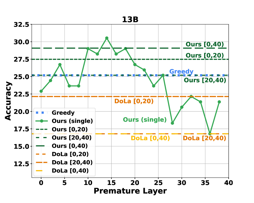
DoLa selects a subset of early layers to form a candidate set. Then it calculates the Jensen-Shannon Divergence (JSD) between the final layer and each layer in this set. Their strategy is to choose the layer with the highest JSD as the premature layer, and the chosen layer will be contrasted with the final layer to update probabilities. Obviously, if this strategy is reasonable, a larger candidate set should lead to a better choice of the premature layer and, consequently, enhanced overall performance. However, a paradoxical finding from their experimental results, which our tests also confirm in the discussion in Section 3.5, is that a larger candidate set for DoLa leads to decreased performance. Specifically, when the candidate set for DoLa ranged from 0 to 32 layers for LLaMA-2-7B-Base, the performance was inferior compared to a smaller set of 0 to 16 layers. This fundamental flaw indicates that selecting a good candidate set remains a challenge when applying DoLa. In contrast, our method does not face this concern as it applies an ensemble approach to all early layers. It is also important to note that our method works well even when only contrasting the final layer with part of the early layers, as demonstrated in Section 3.5 and A, proving the robustness of our approach.

Q 2.2: Why not use $\mathcal{P}_{\mathit{latent}}$ directly as the model’s output distribution?

It is crucial to understand that $\mathcal{P}_{\mathit{latent}}$ is merely an estimation of the real-world distribution based on the model’s latent knowledge instead of the exact $\mathcal{P}_{\mathit{real}}$. Consequently, relying solely on $\mathcal{P}_{\mathit{latent}}$, similar to DoLa, might lead to inaccuracies, as the latent knowledge can be imperfect. The original logits $\mathit{logits}_{\mathit{N}}$ are still important as they are refined directly by real-world data during training. The evolution rate $\alpha$ in Equation 2, serves to balance this trade-off, enabling a reciprocal enhancement between $\mathcal{P}_{\mathit{latent}}$ and the original $\mathit{logits}_{\mathit{N}}$. More ablation studies are provided in Section 3.5 and A.

Q 2.2: Considering that SLED adopts $\mathit{logits}_{\mathit{n}}-\mathit{logits}_{\mathit{N}}$ as the estimation of the gradient, why not directly apply it in Equation 2?

It is important to note that while $\mathit{logits}_{\mathit{n}}-\mathit{logits}_{\mathit{N}}$ is unconstrained, the gradients estimated in Equation 2 (e.g., $p_{(1,\mathit{N})}-m_{1},\ldots,p_{(d,\mathit{N})}-m_{d})$ are constrained within $[-1,1]$. Thus, direct substitution could lead to a mismatch in magnitudes and might also introduce unexpected noise. Proper normalization and subsequent aggregation of estimations from different layers are precisely what our method addresses in Section 2.2 and 2.3. Further analysis is provided in Section A.

3 Experiments

As a novel layer-wise contrastive decoding approach, we first benchmark SLED against the state-of-the-art approach DoLa [7] across a diverse range of model families (LLaMA 2, LLaMA 3, Gemma) and model scales (from 2B to 70B), including the more advanced mixture of experts (MoE) architecture, as detailed in Section 3.2 and 3.3. The results showcase notable factuality improvements across a variety of tasks, including multi-choice, open-generation, and adaptations to chain-of-thought reasoning tasks. Then, in Section 3.4, we integrate our method with other established factuality decoding techniques, illustrating that SLED can further enhance their performance. In Section 3.5, we further conduct in-depth studies on mitigating the repetition issue, layer selection, various parameter settings, and latency overhead to gain more comprehensive insights into SLED’s performance. We also extend our analysis with additional ablation studies and results across more benchmarks in Section A and C in the Appendix, and provide several examples of generated text as the qualitative study in Section B.

3.1 Experimental Setup

Benchmarks

We compare our method with baselines on several multiple-choice and open-ended generation tasks. For multiple-choice question tasks, we use the TruthfulQA [29] and FACTOR (Wiki)  [33] datasets to assess the LLMs’ factuality in short-answer/long-paragraph scenario, respectively. For open-ended generation tasks, we adopt TruthfulQA  [29] and tasks involving chain-of-thought reasoning [52]: StrategyQA [12] and GSM8K [8].

Models & Baselines

We evaluate the performance of SLED on six LLaMA-2 models [48] ({7B,13B,70B}-Base, {7B,13B,70B}-Chat), four LLaMA-3 family models [1] ({8B,70B}-Base, {8B,70B}-IT), two Gemma models (2B,7B), two MoE models (Mixtral-8$\times$7B, Mixtral-8$\times$7B-IT) [18]. We adopt the following baselines: 1) standard decoding (greedy decoding or sampling depending on the tasks), 2) DoLa [7], 3) Inference Time Intervention (ITI) [26], 4) Activation Decoding (AD) [4], 5) Contrastive Decoding (CD)  [27], and 6) Induce-then-Contrast Decoding (ICD) [64].

Metrics

We adopt the factual accuracy evaluation implemented in  [7] for multiple-choice tasks and chain-of-thought reasoning tasks. For the open-ended generation task on TruthfulQA, we follow the evaluation procedure in  [7, 29], using “finetuned-GPT3-judge”s to measure the truthfulness, informativeness, and rejection rate of generated outputs respectively.

Table 1: Comparison on LLaMA 2 model family. The best results are in bold for each dataset/metric. SLED outperforms DoLa and vanilla greedy decoding.

Model&Method	TruthfulQA (MC)			FACTOR	TruthfulQA (Open-Ended)				CoT
	MC1	MC2	MC3		%Truth	%Info	%T*I	%Reject	StrQA	GSM8K
LLaMA-2-7B-Base	33.17	59.42	31.78	58.15	32.80	90.09	23.99	8.45	60.96	14.03
+DoLa	32.56	63.03	30.57	62.49	35.74	95.23	32.31	2.57	60.61	14.71
+SLED (ours)	34.15	62.57	31.89	67.27	55.81	94.61	52.87	0.12	61.31	15.01
LLaMA-2-7B-Chat	35.62	57.46	32.07	56.78	59.24	78.95	38.68	17.50	63.67	21.08
+DoLa	33.41	61.93	30.35	56.65	58.02	87.03	45.78	13.10	64.32	21.00
+SLED (ours)	37.08	63.86	32.90	64.70	67.07	88.13	55.69	11.02	64.67	21.15
LLaMA-2-13B-Base	33.69	62.75	31.74	63.69	31.21	91.55	23.26	7.96	66.07	28.66
+DoLa	29.25	62.13	30.29	57.08	37.58	92.41	30.11	7.47	65.55	18.88
+SLED (ours)	34.15	63.62	31.89	70.91	38.31	94.85	33.29	5.02	66.81	29.34
LLaMA-2-13B-Chat	36.47	63.05	32.77	62.06	60.34	86.54	47.12	13.59	69.87	36.47
+DoLa	34.52	63.24	31.48	58.08	60.22	90.33	51.16	9.67	67.90	34.57
+SLED (ours)	37.09	63.75	32.60	67.50	63.65	95.23	58.87	5.26	69.96	36.54
LLaMA-2-70B-Base	33.66	61.10	32.33	72.78	55.45	62.55	18.48	36.74	75.20	56.33
+DoLa	26.93	60.33	29.42	61.92	60.95	70.62	32.07	17.72	73.45	43.37
+SLED (ours)	35.13	64.92	33.52	77.49	59.24	82.99	43.70	13.10	75.20	57.09
LLaMA-2-70B-Chat	35.98	64.18	32.99	69.07	49.57	81.27	31.33	29.13	77.25	54.59
+DoLa	31.58	54.40	32.31	58.28	61.44	77.97	39.90	21.28	74.41	49.05
+SLED (ours)	38.31	66.71	34.66	73.98	62.55	84.70	47.74	14.98	77.38	54.81

3.2 Evaluation on a Broad Range of LLM Benchmarks

Table 2: Using SLED with other LLM families also improves the factuality.

Model	FACTOR	TruthfulQA			Model	FACTOR	TruthfulQA
		MC1	MC2	MC3			MC1	MC2	MC3
LLaMA-3-8B	64.33	33.78	63.00	32.59	Mixtral-8$\times$7B	71.41	35.13	49.98	34.17
+DoLa	68.04	33.29	63.35	32.16	+DoLa	58.28	32.44	35.91	33.68
+SLED (ours)	68.67	35.13	64.09	32.50	+SLED (ours)	74.92	35.86	57.26	32.96
LLaMA-3-8B-IT	59.49	38.92	68.16	36.50	Mixtral-8$\times$7B-IT	70.51	37.94	62.51	35.25
+DoLa	61.06	35.86	65.30	33.78	+DoLa	56.15	32.19	39.17	33.76
+SLED (ours)	67.17	42.23	69.03	37.97	+SLED (ours)	75.55	41.73	68.52	37.70
LLaMA-3-70B	78.72	35.62	65.66	34.18	Gemma-2B	50.87	23.38	37.16	17.42
+DoLa	77.56	33.29	64.83	32.81	+DoLa	32.93	26.07	48.97	26.55
+SLED (ours)	80.83	37.58	66.19	34.11	+SLED (ours)	57.05	25.21	50.20	26.94
LLaMA-3-70B-IT	73.95	44.80	70.29	41.02	Gemma-7B	60.42	31.58	47.63	22.75
+DoLa	71.51	38.43	68.70	35.21	+DoLa	36.07	25.21	43.14	26.13
+SLED (ours)	76.85	48.35	74.03	43.16	+SLED (ours)	65.56	32.31	49.88	25.22

Multiple-Choices Tasks

The objective of these tasks is to employ decoding methods that enable LLMs to assign higher probabilities to correct completions/answers over incorrect alternatives. We demonstrate the effectiveness of SLED for both Short-Answer Factuality on the TruthfulQA and Long-Paragraph Factuality on the FACTOR dataset. For both DoLa and our SLED, we contrast the results from the final layer against all preceding layers. We randomly sample approximately 5% of the data for validation regarding parameter selection. The results, as shown in Table 1, indicate that SLED achieves superior outcomes in almost all metrics across six LLaMA-2 models. Notably, SLED achieves better performance under the MC1/MC3 metrics on TruthfulQA, which are more sensitive to fluctuations and pose a greater challenge. For long sentences in FACTOR, our method shows improvements over baselines by 5-13%. These results not only underscore the benefits of our method for factuality but also demonstrate its robustness across different lengths of text.

Open-Ended Generation Tasks

In open-ended settings, we prompt the model to generate answers for the same questions from TruthfulQA, following the settings outlined in [29, 7, 27]. In Table 1, we compare the performance of six LLaMA-2 models using standard greedy decoding, (greedy) DoLa, and (greedy) SLED. All the generated answers are then evaluated by a fine-tuned GPT-3 model for both truthfulness and informativeness scores. Considering that a 100% truthful score can be easily achieved by simply responding with ’I have no comment,’ which would result in a 0% informative score and thus is not very useful, we have introduced additional metrics—%Truth $\times$ Info and the rejection ratio %Reject —to demonstrate that SLED is a mutual-gains approach to achieve better both truthful and informative scores. We have improved the overall %Truth x Info scores by 3-20% across different models and reduced the rejection ratio by up to 95%. These enhancements demonstrate that our method effectively avoids the ’rejection pitfall,’ making it more helpful.

Adaptation to Chain-of-thought Reasoning Tasks

Although the StrategyQA and GSM8K tasks are also open-ended and require factual accuracy, the primary focus here is to evaluate how different decoding methods adapt to the Chain-of-Thought (COT) approach for handling complex reasoning tasks. We maintain a repetition penalty of 1, as we will discuss the repetition flaws associated with DoLa in Section 3.5. StrategyQA demands multi-hop reasoning, and as shown in Table 1, our method boosts accuracy across six models, whereas DoLa generally worsens it without a repetition penalty. GSM8K, a benchmark for math word problems that require arithmetic reasoning, also shows consistent accuracy improvement with SLED in 7B, 13B and 70B models.

3.3 Evaluation Across Diverse LLM Configurations

As discussed above and shown in Table 1, our method, SLED, demonstrates strong generalization capabilities across the LLaMA-2 model family, proving robust from 7B to 70B model sizes. In Table 2, we further showcase SLED’s impressive performance on the more recent LLaMA-3 family models, both at 8B and 70B sizes, in terms of long paragraph factuality and short answer factuality. Interestingly, SLED is also applicable to different pre-trained models, such as Gemma at both 2B and 7B sizes, and can even be adapted to the increasingly popular Mixture of Experts (MoE) architectures. These results confirm the exceptional adaptability of our method across various LLM configurations.

3.4 Evaluation on Integrating SLED with Other LLM Factuality Decoding Methods

SLED exclusively focuses on contrasting differences between layers without altering other parts of the model. Thus, it remains compatible with other techniques that incorporate additional strategies or utilize auxiliary models. This compatibility allows SLED to be seamlessly integrated into existing methods, enhancing factuality further without the need for modifications to SLED. We integrate SLED with the following approaches: ITI, AD, CD and ICD. Table 3 shows that SLED leads to accuracy improvements from 1% to 12% across four LLaMA-2 models.

Table 3: Comparison of decoding strategies on TruthfulQA datasets. SLED can also be seamlessly combined with other decoding strategies to improve performance further.

Model	LLaMA-2-7B-base			LLaMA-2-7B-chat
Method	AD	AD +DoLa	AD +SLED	AD	AD +DoLa	AD +SLED	ITI	ITI +SLED	ICD	ICD +SLED
MC1	32.80	25.58	33.29	35.37	33.41	36.23	36.60	43.33	46.32	46.87
MC2	59.59	39.06	62.55	58.14	50.31	63.15	65.62	65.75	69.08	72.09
MC3	31.05	17.89	31.80	31.84	23.15	32.23	34.89	37.66	41.25	43.64

Model	LLaMA-2-13B-base					LLaMA-2-13B-chat
Method	AD	AD +DoLa	AD +SLED	CD	CD +SLED	AD	AD +DoLa	AD +SLED	CD	CD +SLED
MC1	33.90	24.72	33.90	30.11	33.78	36.84	34.72	36.35	28.15	36.47
MC2	62.93	37.74	63.69	50.31	63.22	63.75	50.42	64.83	54.87	64.93
MC3	31.61	17.66	31.38	28.18	32.21	32.69	23.83	32.85	29.75	33.39

Table 4: Accuracy of LLaMA 2 13B Base on StrategyQA with Varying Repetition Penalties

Metric	Method	1	1.02	1.04	1.06	1.08	1.1	1.2	2
Accuracy(%)	DoLa	65.55	65.98	66.37	65.98	65.59	66.37	67.16	66.64
	SLED (Ours)	66.81	69.39	68.51	68.47	67.07	65.72	60.87	54.75
Repetition-4(%)	DoLa	7.63	7.19	6.45	5.98	5.50	5.10	3.73	2.05
	SLED (Ours)	3.73	2.45	1.89	1.36	1.05	0.69	0.20	0.10
Repetition-Sen(%)	DoLa	2.16	2.04	1.66	1.37	1.12	0.89	0.23	0.03
	SLED (Ours)	0.88	0.39	0.10	0.02	0.03	0	0	0

3.5 Ablation Studies and Analysis

Mitigating Repetition Issues

Table 4 demonstrates that our method, SLED, effectively addresses a significant issue in DoLa: repetitive content in open-ended generation tasks. Our approach outperforms DoLa without the need for excessive repetition penalty. While a slight increase in the repetition penalty further enhances the performance of our method, excessive penalties, such as 1.1, tend to degrade it. This suggests that SLED does not inherently require heavy adjustments for repetition issues. In contrast, DoLa’s performance improves with higher penalties (e.g., 1.1, 1.2, 2), indicating a more critical need for addressing repetitive content. We also employ two intuitive metrics, Repetition-4 and Repetition-Sen, to gauge the severity of repetition issues, following prior research [55]. Regardless of the repetition penalty imposed, our method consistently exhibits lower repetition rates. Table 7 includes some examples of generated text to illustrate this further.

Layer Selection

As discussed in Section 2.4, how to choose a good candidate set is still a paradoxically difficult task when applying DoLa. Our method does not exhibit this issue. Instead of selecting a single premature layer from the candidate set like DoLa, SLED contrasts the final layer with all layers in the candidate set and then ensembles all the results. Figure 5 shows that setting a larger candidate set, such as all the 32 layers for LLaMA-2-7B-Base, yields better performance than focusing solely on either the first $[0,16)$ or second half $[16,32)$. This implies that our layer-wise contrast approach captures more useful information in a more scientific manner. Furthermore, our tests confirm the robustness of our method even when the candidate set is minimal, such as a single layer, consistently demonstrating strong performance. Our settings mirror those of DoLa.

Figure 5: Evaluating using different premature layers for SLED and DoLa on a 10% subset of the GSM8K dataset. Contrasting all layers for SLED is better than using only the first half [0, 16) or the second half [16, 32). Hence, there are no improvements for SLED from strategic layer subset selection.

Parameter Analysis

Figure 6: WE explore the impact of evolution scale and rate based on the factual accuracy of a subset of the FACTOR dataset. (G: Greedy, D: DoLa)

(a) LLaMA 2 7B Base

(b) LLaMA 2 7B Chat

(c) LLaMA 2 13B Base

(d) LLaMA 2 13B Chat

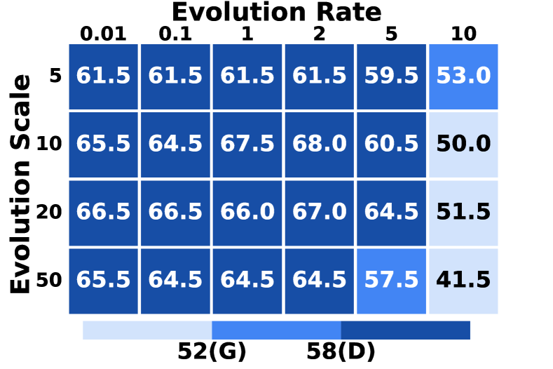
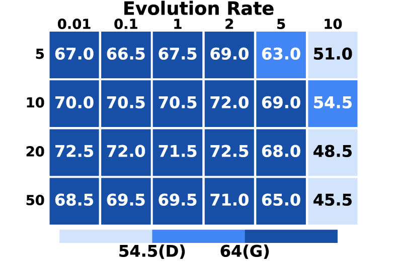
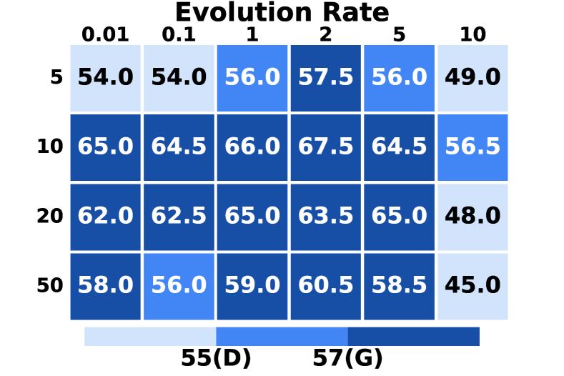
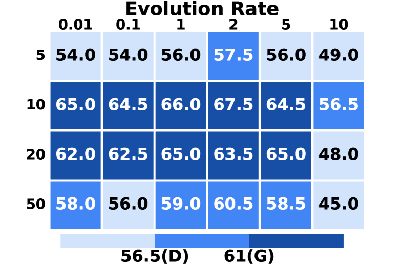
We next investigate the impact of parameters — evolution rate $\alpha$ and evolution scale $k$ — on the performance of SLED using a subset of the FACTOR dataset. We test evolution rates from $\{0.01,0.1,1,2,5,10\}$ and evolution scale values from $\{5,10,20,50\}$. Without extreme evolution rates (e.g., 10), our method performs well, confirming its robustness. As analyzed in our methodology and Eq. 2, the evolution rate balances the logit distribution ($\mathcal{P}_{\mathcal{N}})$ with the latent knowledge distribution ($\mathcal{P}_{\mathit{latent}}$). A lower evolution rate works better for larger models (13B) and chat models as their logits already better represent real-world distributions.

Latency

Our method, SLED, does not incur significant latency overhead. The latencies presented in Table 5 demonstrate that our method, SLED, just increases the decoding time of DoLa by factors ranging from 0.1% to 10%. Notably, even with an atypical setting such as evolution scale $=100$, which is seldom used, the increase remains around 10%. The latency for DoLa and SLED is much higher compared to the vanilla greedy decoding because we set all early layers as candidate layers set for both DoLa and SLED for a fair comparison.

Table 5: Latency (ms/token) comparison across different configurations. (ES: evolution scale)

Model	Greedy	DoLa	SLED (ES=5)	SLED (ES=20)	SLED (ES=50)	SLED (ES=100)
LLaMA-2-7B	23.64	29.93	30.41	31.15	32.70	34.63
LLaMA-2-13B	30.41	39.57	39.61	41.14	43.30	45.09
LLaMA-2-70B	82.63	136.42	138.33	140.24	143.12	148.85

4 Related Work

There have been many advances in improving training and inference to develop better out-of-the-box LLMs [47, 48, 1, 44, 36, 28, 63, 51, 20]. Unfortunately, LLMs still suffer from hallucinations and producing non-factual text. This has led researchers to develop many methods to improve factuality.

Retrieval, Fine-tuning, and Preferences.

Many techniques use additional knowledge graphs or fine-tuning data to increase factuality by updating the model parameters for this goal. One method is Retrieval-Augmented Generation (RAG) to use external knowledge to improve generation [3, 5, 9, 25]. Another option is to use post-generation retrieval and editing for improving attribution [11]. Other directions that use additional training or preference data are supervised fine-tuning (SFT) [38, 46], RLHF [37], DPO [40] or self-rewarding [58]. Complementary to these approaches, we wish to improve the LLM output distribution directly without needing any additional data.

Decoding and Factuality Decoding

For each prefix, the LLM generates a probability distribution for the next token on a fixed vocabulary list, and a decoding method determines how the next token is derived based on the estimated distribution. Decoding methods were initially developed to enhance the fluency and coherence of text generation, such as Beam Search (BS), which maintains the $k$ most probable sequences at each time step. Common decoding methods also include Diverse Beam Search (DBS) [49], Contrastive Decoding [27], Top-p Sampling [14] and so on.

Recently, the potential of decoding has extended beyond merely improving text readability, with some factuality decoding methods being proposed. These methods modify the generation process to focus on truthful statements rather than unsupported claims during the inference phase, aiming to reduce hallucinations. Notable recent works include Inference-Time Intervention (ITI) [26], Induced-Contrastive Decoding [64], Decoding by Contrasting Layers (DoLa) [7] and so on. ITI adjusts model activations during inference by following learned directions across a limited number of attention heads to improve truthfulness. Some researchers have extended previous Contrastive Decoding [27] methods to improve factual accuracy, such as Frustratingly Easy Model Decoding [56] and Induced-Contrastive Decoding [64], leveraging differences between expert and amateur models. Most closely related to our work is DoLa, which also employs contrasting logits from different layers. However, significant distinctions exist: Firstly, our method diverges in how to utilize those differences between logits to extract latent knowledge. Secondly, whereas DoLa directly substitutes the original output distribution with the latent knowledge distribution, our approach recognizes potential inaccuracies in this estimated distribution and adopts gradient descent within an optimization framework to integrate the model’s latent knowledge with the original output.

Limitations.

As we continue to refine our approach, several aspects of our method can be further developed and enhanced. Our method, SLED, achieves better factuality at the cost of operating slightly slower. Ideally, we could improve the output logits without incurring any computational cost compared to performing inference on the base LLM model. Another aspect is that currently, our experimental results support the superiority of SLED on multiple datasets. Parameter optimization using Bayesian methods [54, 30, 60, 61, 66], evolutionary algorithms [16, 32, 41] or reinforcement learning [67, 6, 19, 39] might also lead to more robust performance. It would also be ideal to back up our results with more theoretical analysis of SLED.

5 Conclusion

We introduced Self Logits Evolution Decoding (SLED), which is a new method to improve accuracy and factuality without requiring external knowledge (e.g., RAG) or fine-tuning (e.g., SFT). The key idea is to optimize the output logits based on the LLMs’ latent knowledge to improve factuality during inference. On several datasets, SLED achieved the SOTA results, improving over the vanilla decoding and DoLa. We also show that SLED does not increase the inference time significantly and that it can be combined with other factuality decoding methods. For future work, it would be interesting to combine SLED with supervised fine-tuning methods, e.g., to adapt to other domains.

Appendix A Additional Analysis and Ablation Studies

Justification on the Gradients Approximation of SLED in Section 2.2

To further support our method’s mechanism, which utilizes $\mathit{logits}_{\mathit{n}}-\mathit{logits}_{\mathit{N}}$ to approximate the gradient of $KL(\mathcal{P}_{\mathit{real}},\mathcal{P}_{\mathit{logits}})$ at $\mathit{logits}=\mathit{logits}_{\mathit{n}}$, we manually calculate the $Cosine\_similarity(\mathit{logits}_{\mathit{n}}-\mathit{logits}_{\mathit{N}},\nabla_{\mathit{logits}}KL(\mathcal{P}_{\mathit{real}},\mathcal{P}_{\mathit{logits}})|_{\mathit{logits}=\mathit{logits}_{\mathit{n}}})$ among thousands of tokens and layers. We plot the density function for different models. We find that the majority of these values are positive, demonstrating that the directions of these two vectors are very close. Hence, our gradient approximation strategy in Section 2.2 is reasonable.

Figure 7: We collect 10k pairs of $(\mathit{logits}_{\mathit{n}}-\mathit{logits}_{\mathit{N}},\nabla_{\mathit{logits}_{\mathit{n}}}KL(\mathcal{P}_{\mathit{real}},\mathcal{P}_{\mathit{logits}_{\mathit{n}}}))$ on different tokens in FACTOR and different early layers. We calculate their cosine similarity values and draw the density function for each LLM. Most of the pairs have positive Cosine similarity values, which verifies that the approximation strategy of SLED is reasonable.

Further Ablation Studies for Section 2.4

We design the following two ablation studies to support our claims in Section 2.4. The first study, referred to as ’Ablation 1’, directly employs $\mathcal{P}_{\mathit{latent}}$ as the output distribution as discussed in Q 2.2. The second study, denoted as ’Ablation 2’, involves directly scaling the differences, $\{\mathit{logits}_{\mathit{n}}-\mathit{logits}_{\mathit{N}}\}$, to constrain their magnitudes within $[-1,1]$. Then, we simply average these scaled differences across different layers and apply them to Equation 2 as mentioned in Q 2.3. The results presented in Table 6 demonstrate that the design of our SLED is reasonable.

	FACTOR	TruthfulQA
		MC1	MC2	MC3
LLaMA-2-7B-Chat + Ablation 1	63.59	25.21	51.09	26.25
+ Ablation 2	62.73	33.66	39.83	31.47
+ SLED	65.16	37.08	63.86	32.90
LLaMA-2-13B-Chat + Ablation 1	66.70	27.05	52.72	28.46
+ Ablation 2	66.29	37.33	45.00	31.98
+ SLED	67.06	37.09	63.75	32.60

Table 6: Performance comparison of ablation studies and SLED on FACTOR and TruthfulQA.

Appendix B Qualitative Studies

We present some examples from the StrategyQA dataset in Table 7 to illustrate that our method addresses the repetition issue of DoLa.

Q: Can you buy a fair trade laptop?
DoLa	A laptop is a portable computer. A portable computer is a handheld computer. A handheld computer is a palmtop computer. A palmtop computer is a PDA. A PDA is a personal digital assistant. A personal digital assistant is a PDA. A PDA is a handheld computer. A handheld computer is a palmtop computer. A palmtop computer is a PDA. A PDA is a personal digital assistant. A personal digital assistant is a PDA. Thus, a PDA is a PDA. A PDA is a PDA. A PDA is a PDA. A PDA is a PDA. A PDA is a PDA. A PDA is a PDA …
SLED	Fair Trade is a certification for coffee. Laptops are not coffee. Thus, you cannot buy a fair trade laptop. So the answer is no.
Q: Can you see the moon in Wembley Arena?
DoLa	Wembley Arena is in London, England. The moon is a celestial body, and the moon is in the sky. The moon is in the sky, and Wembley Arena is in London, England. London, England is on Earth, and the moon is in the sky. The moon is in the sky, and Wembley Arena is on Earth. Wembley Arena is on Earth, and the moon is in the sky. The moon is in the sky, and Wembley Arena is on Earth. The moon is in the sky, and Wembley Arena is on Earth. Wembley Arena is on Earth, and the moon is in the sky. The moon is in the sky, and Wembley Arena is on Earth. Wembley Arena is on Earth, and the moon is in the sky. The moon is in the sky, and Wembley Arena is on Earth. Wembley Arena is on Earth, and the moon is in the sky. The moon is in the sky, and Wembley Arena is on Earth. Wembley Arena is on Earth, and the moon is in the sky. The moon is in the sky, and Wembley Arena is on Earth. Wembley Arena
SLED	Wembley Arena is in London. London is in the Northern Hemisphere, and the moon is in the Southern Hemisphere. Thus, you cannot see the moon in Wembley Arena. So the answer is no.
Q: Does Thiago Moises May 13 2020 submission move hypothetically hurt Achilles?
DoLa	Thiago Moises is a MMA fighter. He is 1.73 m tall, and Achilles is about 0.00000000000000000000000000000000000000000000000000000000000000000000…
SLED	Thiago Moises’s submission was a rear naked choke, which is a blood choke. A blood choke can cause a fighter to pass out. Thus, Thiago Moises’s submission could hypothetically hurt Achilles. So the answer is yes.

Table 7: We present three examples of the generated text from LLaMA-2-13B-Base on StrategyQA dataset. SLED method can mitigate the repetition issue.

Appendix C Further Results from Open-ended Generation Task Benchmarks

We have conducted additional experiments on more realistic open-ended generations datasets, HotPotQA [57], Natural Question (NQ) [23], TriviaQA [21]. We adopt the Exact Match(EM) and the F1 score. Different from the setting in the Section 3, we adopt $[0,2,4,6,8,10,12,14]$ as candidate layers for LLaMA 2 7B Chat model and $[0,2,4,6,8,10,12,14,18]$ as candidate layers for LLaMA 2 13B Chat model for both DoLa and SLED. Our method still has robust performance across different datasets and metrics.

Table 8: Performance comparison on HotPotQA, Natural Question (NQ) and TriviaQA.

Model	HotpotQA		NQ		TriviaQA
	EM	F1	EM	F1	EM	F1
LLaMA 2 7B Chat	19.6	20.1	21.8	20.4	44.4	44.3
+ DoLa	20.4	21.3	23.5	21.5	45.2	45.3
+ SLED (ours)	20.9	21.5	24.4	22.2	47.6	46.3
Llama 2 13B Chat	23.8	21.7	33.1	28.9	63.0	60.9
+ DoLa	24.5	23.2	33.1	28.9	63.2	61.5
+ SLED (ours)	25.0	24.5	34.6	31.6	63.3	62.2

Appendix D Implementation Details

We conducted all experiments utilizing NVIDIA A100 GPUs and implemented our method based on the following repositories: DoLa, AD, and ICD. For decoding responses from the LLMs on TruthfulQA, StrategyQA, and GSM8K, we employed greedy decoding. The models were operated with 16-bit floating-point precision and a batch size of 1. For the LLaMA 2 models sized 7B, 13B, and 70B, we utilized 1, 1, and 3 GPUs respectively. Cross-GPU inference, involving model weight sharding, was facilitated by the Hugging Face Accelerate package.

Regarding the details in Section 3.4, we evaluate the 7B-chat model for ITI, as the checkpoint is publicly available. Combining ITI with SLED results in better performance compared to using ITI alone. AD employs an entropy-based metric to measure the ‘sharpness’ of in-context hidden states and incorporates it into the decoding process. Combining AD with SLED surpasses both the original AD and its combination with DoLa across four model types. For CD, we have conducted experiments in two distinct configurations: (i) the LLaMA 2 13B base model is contrasted with that of the Llama 2 7B base model, and (ii) the LLaMA 2 13B chat model and the LLaMA 2 7B chat model are compared. Applying SLED to the larger models (13B) boosts performance beyond vanilla CD. ICD contrasts a trustworthy 7B model with a fine-tuned, untrustworthy 7B model, and again, applying SLED on the trustworthy 7B model improves factual accuracy further.

Appendix E Additional Results of DoLa

Table 9 presents some additional results of DoLa across various benchmarks. Specifically, DoLa in Table 9 selects a subset of early layers as candidates for calculating the Jensen-Shannon Divergence (JSD) instead of using all layers. For example, for the LLaMA 2 7B Chat model, layers $[0,2,4,6,8,10,12,14]$ are designated as candidate layers. Notably, a specific trick implemented in DoLa is omitting the post-softmax step on logits for the TruthfulQA multiple-choice task to enhance accuracy. This trick is not applied to the vanilla greedy decoding in Table 9. In contrast, for the results presented in our Tables 1, 2, and 3, this technique is also been applied to vanilla greedy decoding to ensure a fair comparison.

Table 9: The Performance of DoLa Across Various Benchmarks

Model	TruthfulQA			GSM8K	StrQA
	MC1	MC2	MC3
LLaMA-2-7B-Base	28.40	43.39	20.52	14.03	60.96
+ DoLa	31.21	62.12	29.73	14.63	60.74
LLaMA-2-13B-Base	29.01	44.27	20.71	28.66	66.07
+ DoLa	29.38	63.95	33.63	28.81	66.59
LLaMA-2-70B-Base	37.70	53.60	27.36	56.33	75.20
+ DoLa	27.05	60.26	31.64	56.94	74.93
LLaMA-2-7B-Chat	33.66	51.29	24.91	21.08	63.67
+ DoLa	33.29	60.86	29.77	20.55	64.37
LLaMA-2-13B-Chat	35.37	53.31	26.71	36.47	69.87
+ DoLa	31.95	62.44	31.23	35.79	69.48
LLaMA-2-70B-Chat	37.33	56.33	27.94	54.59	77.25
+ DoLa	31.33	54.48	34.43	54.44	76.86

References

- AI@Meta [2024] AI@Meta. Llama 3 model card. 2024. URL https://github.com/meta-llama/llama3/blob/main/MODEL_CARD.md.
- Anil et al. [2023] Rohan Anil, Andrew M Dai, Orhan Firat, Melvin Johnson, Dmitry Lepikhin, Alexandre Passos, Siamak Shakeri, Emanuel Taropa, Paige Bailey, Zhifeng Chen, et al. Palm 2 technical report. arXiv preprint arXiv:2305.10403, 2023.
- Chen et al. [2024a] Jiawei Chen, Hongyu Lin, Xianpei Han, and Le Sun. Benchmarking large language models in retrieval-augmented generation. In Proceedings of the AAAI Conference on Artificial Intelligence, volume 38, pages 17754–17762, 2024a.
- Chen et al. [2024b] Shiqi Chen, Miao Xiong, Junteng Liu, Zhengxuan Wu, Teng Xiao, Siyang Gao, and Junxian He. In-context sharpness as alerts: An inner representation perspective for hallucination mitigation. arXiv preprint arXiv:2403.01548, 2024b.
- Cheng et al. [2024] Xin Cheng, Di Luo, Xiuying Chen, Lemao Liu, Dongyan Zhao, and Rui Yan. Lift yourself up: Retrieval-augmented text generation with self-memory. Advances in Neural Information Processing Systems, 36, 2024.
- Christiano et al. [2017] Paul Francis Christiano, Jan Leike, Tom B. Brown, Miljan Martic, Shane Legg, and Dario Amodei. Deep reinforcement learning from human preferences. ArXiv, abs/1706.03741, 2017.
- Chuang et al. [2024] Yung-Sung Chuang, Yujia Xie, Hongyin Luo, Yoon Kim, James R. Glass, and Pengcheng He. Dola: Decoding by contrasting layers improves factuality in large language models. In The Twelfth International Conference on Learning Representations, 2024. URL https://openreview.net/forum?id=Th6NyL07na.
- Cobbe et al. [2021] Karl Cobbe, Vineet Kosaraju, Mohammad Bavarian, Mark Chen, Heewoo Jun, Lukasz Kaiser, Matthias Plappert, Jerry Tworek, Jacob Hilton, Reiichiro Nakano, et al. Training verifiers to solve math word problems. arXiv preprint arXiv:2110.14168, 2021.
- Ding et al. [2024] Yujuan Ding, Wenqi Fan, Liangbo Ning, Shijie Wang, Hengyun Li, Dawei Yin, Tat-Seng Chua, and Qing Li. A survey on rag meets llms: Towards retrieval-augmented large language models. arXiv preprint arXiv:2405.06211, 2024.
- Du et al. [2024] Yilun Du, Shuang Li, Antonio Torralba, Joshua B. Tenenbaum, and Igor Mordatch. Improving factuality and reasoning in language models through multiagent debate, 2024. URL https://openreview.net/forum?id=QAwaaLJNCk.
- Gao et al. [2023] Luyu Gao, Zhuyun Dai, Panupong Pasupat, Anthony Chen, Arun Tejasvi Chaganty, Yicheng Fan, Vincent Zhao, Ni Lao, Hongrae Lee, Da-Cheng Juan, and Kelvin Guu. RARR: Researching and revising what language models say, using language models. In Anna Rogers, Jordan Boyd-Graber, and Naoaki Okazaki, editors, Proceedings of the 61st Annual Meeting of the Association for Computational Linguistics (Volume 1: Long Papers), pages 16477–16508, Toronto, Canada, July 2023. Association for Computational Linguistics. doi: 10.18653/v1/2023.acl-long.910. URL https://aclanthology.org/2023.acl-long.910.
- Geva et al. [2021] Mor Geva, Daniel Khashabi, Elad Segal, Tushar Khot, Dan Roth, and Jonathan Berant. Did aristotle use a laptop? a question answering benchmark with implicit reasoning strategies. Transactions of the Association for Computational Linguistics, 9:346–361, 2021.
- Hinton et al. [2015] Geoffrey Hinton, Oriol Vinyals, Jeff Dean, et al. Distilling the knowledge in a neural network. arXiv preprint arXiv:1503.02531, 2(7), 2015.
- Holtzman et al. [2019] Ari Holtzman, Jan Buys, Li Du, Maxwell Forbes, and Yejin Choi. The curious case of neural text degeneration. arXiv preprint arXiv:1904.09751, 2019.
- Huang et al. [2023] Lei Huang, Weijiang Yu, Weitao Ma, Weihong Zhong, Zhangyin Feng, Haotian Wang, Qianglong Chen, Weihua Peng, Xiaocheng Feng, Bing Qin, et al. A survey on hallucination in large language models: Principles, taxonomy, challenges, and open questions. arXiv preprint arXiv:2311.05232, 2023.
- Jaderberg et al. [2017] Max Jaderberg, Valentin Dalibard, Simon Osindero, Wojciech M Czarnecki, Jeff Donahue, Ali Razavi, Oriol Vinyals, Tim Green, Iain Dunning, Karen Simonyan, et al. Population based training of neural networks. arXiv preprint arXiv:1711.09846, 2017.
- Ji et al. [2023] Ziwei Ji, Nayeon Lee, Rita Frieske, Tiezheng Yu, Dan Su, Yan Xu, Etsuko Ishii, Ye Jin Bang, Andrea Madotto, and Pascale Fung. Survey of hallucination in natural language generation. ACM Computing Surveys, 55(12):1–38, 2023.
- Jiang et al. [2024] Albert Q. Jiang, Alexandre Sablayrolles, Antoine Roux, Arthur Mensch, Blanche Savary, Chris Bamford, Devendra Singh Chaplot, Diego de las Casas, Emma Bou Hanna, Florian Bressand, Gianna Lengyel, Guillaume Bour, Guillaume Lample, Lélio Renard Lavaud, Lucile Saulnier, Marie-Anne Lachaux, Pierre Stock, Sandeep Subramanian, Sophia Yang, Szymon Antoniak, Teven Le Scao, Théophile Gervet, Thibaut Lavril, Thomas Wang, Timothée Lacroix, and William El Sayed. Mixtral of experts, 2024. URL https://arxiv.org/abs/2401.04088.
- Jomaa et al. [2019] Hadi S Jomaa, Josif Grabocka, and Lars Schmidt-Thieme. Hyp-rl: Hyperparameter optimization by reinforcement learning. arXiv preprint arXiv:1906.11527, 2019.
- Joren et al. [2024] Hailey Joren, Jianyi Zhang, Chun-Sung Ferng, Da-Cheng Juan, Ankur Taly, and Cyrus Rashtchian. Sufficient context: A new lens on retrieval augmented generation systems. arXiv preprint arXiv:2411.06037, 2024.
- Joshi et al. [2017] Mandar Joshi, Eunsol Choi, Daniel Weld, and Luke Zettlemoyer. triviaqa: A Large Scale Distantly Supervised Challenge Dataset for Reading Comprehension. arXiv e-prints, art. arXiv:1705.03551, 2017.
- Kadavath et al. [2022] Saurav Kadavath, Tom Conerly, Amanda Askell, Tom Henighan, Dawn Drain, Ethan Perez, Nicholas Schiefer, Zac Hatfield-Dodds, Nova DasSarma, Eli Tran-Johnson, et al. Language models (mostly) know what they know. arXiv preprint arXiv:2207.05221, 2022.
- Kwiatkowski et al. [2019] Tom Kwiatkowski, Jennimaria Palomaki, Olivia Redfield, Michael Collins, Ankur Parikh, Chris Alberti, Danielle Epstein, Illia Polosukhin, Matthew Kelcey, Jacob Devlin, Kenton Lee, Kristina N. Toutanova, Llion Jones, Ming-Wei Chang, Andrew Dai, Jakob Uszkoreit, Quoc Le, and Slav Petrov. Natural questions: a benchmark for question answering research. Transactions of the Association of Computational Linguistics, 2019.
- Lei et al. [2023] Deren Lei, Yaxi Li, Mengya Hu, Mingyu Wang, Vincent Yun, Emily Ching, Eslam Kamal, et al. Chain of natural language inference for reducing large language model ungrounded hallucinations. arXiv preprint arXiv:2310.03951, 2023.
- Lewis et al. [2020] Patrick Lewis, Ethan Perez, Aleksandra Piktus, Fabio Petroni, Vladimir Karpukhin, Naman Goyal, Heinrich Küttler, Mike Lewis, Wen-tau Yih, Tim Rocktäschel, et al. Retrieval-augmented generation for knowledge-intensive nlp tasks. Advances in Neural Information Processing Systems, 33:9459–9474, 2020.
- Li et al. [2023a] Kenneth Li, Oam Patel, Fernanda Viégas, Hanspeter Pfister, and Martin Wattenberg. Inference-time intervention: Eliciting truthful answers from a language model. In A. Oh, T. Naumann, A. Globerson, K. Saenko, M. Hardt, and S. Levine, editors, Advances in Neural Information Processing Systems, volume 36, pages 41451–41530. Curran Associates, Inc., 2023a. URL https://proceedings.neurips.cc/paper_files/paper/2023/file/81b8390039b7302c909cb769f8b6cd93-Paper-Conference.pdf.
- Li et al. [2022] Xiang Lisa Li, Ari Holtzman, Daniel Fried, Percy Liang, Jason Eisner, Tatsunori Hashimoto, Luke Zettlemoyer, and Mike Lewis. Contrastive decoding: Open-ended text generation as optimization. arXiv preprint arXiv:2210.15097, 2022.
- Li et al. [2023b] Yuanzhi Li, Sébastien Bubeck, Ronen Eldan, Allie Del Giorno, Suriya Gunasekar, and Yin Tat Lee. Textbooks are all you need ii: phi-1.5 technical report. arXiv preprint arXiv:2309.05463, 2023b.
- Lin et al. [2022] Stephanie Lin, Jacob Hilton, and Owain Evans. TruthfulQA: Measuring how models mimic human falsehoods. In Smaranda Muresan, Preslav Nakov, and Aline Villavicencio, editors, Proceedings of the 60th Annual Meeting of the Association for Computational Linguistics (Volume 1: Long Papers), pages 3214–3252, Dublin, Ireland, May 2022. Association for Computational Linguistics. doi: 10.18653/v1/2022.acl-long.229. URL https://aclanthology.org/2022.acl-long.229.
- Liu and Wang [2019] Qiang Liu and Dilin Wang. Stein variational gradient descent: A general purpose bayesian inference algorithm, 2019.
- Mesnard et al. [2024] Gemma Team Thomas Mesnard, Cassidy Hardin, Robert Dadashi, Surya Bhupatiraju, Shreya Pathak, L. Sifre, Morgane Riviere, Mihir Kale, J Christopher Love, Pouya Dehghani Tafti, L’eonard Hussenot, Aakanksha Chowdhery, Adam Roberts, Aditya Barua, Alex Botev, Alex Castro-Ros, Ambrose Slone, Am’elie H’eliou, Andrea Tacchetti, Anna Bulanova, Antonia Paterson, Beth Tsai, Bobak Shahriari, Charline Le Lan, Christopher A. Choquette-Choo, Cl’ement Crepy, Daniel Cer, Daphne Ippolito, David Reid, Elena Buchatskaya, Eric Ni, Eric Noland, Geng Yan, George Tucker, George-Christian Muraru, Grigory Rozhdestvenskiy, Henryk Michalewski, Ian Tenney, Ivan Grishchenko, Jacob Austin, James Keeling, Jane Labanowski, Jean-Baptiste Lespiau, Jeff Stanway, Jenny Brennan, Jeremy Chen, Johan Ferret, Justin Chiu, Justin Mao-Jones, Katherine Lee, Kathy Yu, Katie Millican, Lars Lowe Sjoesund, Lisa Lee, Lucas Dixon, Machel Reid, Maciej Mikula, Mateo Wirth, Michael Sharman, Nikolai Chinaev, Nithum Thain, Olivier Bachem, Oscar Chang, Oscar Wahltinez, Paige Bailey, Paul Michel, Petko Yotov, Pier Giuseppe Sessa, Rahma Chaabouni, Ramona Comanescu, Reena Jana, Rohan Anil, Ross McIlroy, Ruibo Liu, Ryan Mullins, Samuel L Smith, Sebastian Borgeaud, Sertan Girgin, Sholto Douglas, Shree Pandya, Siamak Shakeri, Soham De, Ted Klimenko, Tom Hennigan, Vladimir Feinberg, Wojciech Stokowiec, Yu hui Chen, Zafarali Ahmed, Zhitao Gong, Tris Brian Warkentin, Ludovic Peran, Minh Giang, Cl’ement Farabet, Oriol Vinyals, Jeffrey Dean, Koray Kavukcuoglu, Demis Hassabis, Zoubin Ghahramani, Douglas Eck, Joelle Barral, Fernando Pereira, Eli Collins, Armand Joulin, Noah Fiedel, Evan Senter, Alek Andreev, and Kathleen Kenealy. Gemma: Open models based on gemini research and technology. ArXiv, abs/2403.08295, 2024. URL https://api.semanticscholar.org/CorpusID:268379206.
- Miikkulainen et al. [2024] Risto Miikkulainen, Jason Liang, Elliot Meyerson, Aditya Rawal, Dan Fink, Olivier Francon, Bala Raju, Hormoz Shahrzad, Arshak Navruzyan, Nigel Duffy, et al. Evolving deep neural networks. In Artificial intelligence in the age of neural networks and brain computing, pages 269–287. Elsevier, 2024.
- Muhlgay et al. [2023] Dor Muhlgay, Ori Ram, Inbal Magar, Yoav Levine, Nir Ratner, Yonatan Belinkov, Omri Abend, Kevin Leyton-Brown, Amnon Shashua, and Yoav Shoham. Generating benchmarks for factuality evaluation of language models. arXiv preprint arXiv:2307.06908, 2023.
- Müller et al. [2019] Rafael Müller, Simon Kornblith, and Geoffrey E Hinton. When does label smoothing help? Advances in neural information processing systems, 32, 2019.
- OpenAI [2022] OpenAI. Introducing chatgpt. https://openai.com/blog/chatgpt/, November 2022.
- OpenAI [2023] OpenAI. GPT-4 Technical Report. arXiv e-prints, art. arXiv:2303.08774, March 2023. doi: 10.48550/arXiv.2303.08774.
- Ouyang et al. [2022] Long Ouyang, Jeffrey Wu, Xu Jiang, Diogo Almeida, Carroll Wainwright, Pamela Mishkin, Chong Zhang, Sandhini Agarwal, Katarina Slama, Alex Ray, et al. Training language models to follow instructions with human feedback. Advances in Neural Information Processing Systems, 35:27730–27744, 2022.
- Ovadia et al. [2023] Oded Ovadia, Menachem Brief, Moshik Mishaeli, and Oren Elisha. Fine-tuning or retrieval? comparing knowledge injection in llms. arXiv preprint arXiv:2312.05934, 2023.
- Qi and Xu [2023] Xin Qi and Bing Xu. Hyperparameter optimization of neural networks based on q-learning. Signal, Image and Video Processing, 17(4):1669–1676, 2023.
- Rafailov et al. [2024] Rafael Rafailov, Archit Sharma, Eric Mitchell, Christopher D Manning, Stefano Ermon, and Chelsea Finn. Direct preference optimization: Your language model is secretly a reward model. Advances in Neural Information Processing Systems, 36, 2024.
- Real et al. [2017] Esteban Real, Sherry Moore, Andrew Selle, Saurabh Saxena, Yutaka Leon Suematsu, Jie Tan, Quoc V Le, and Alexey Kurakin. Large-scale evolution of image classifiers. In International conference on machine learning, pages 2902–2911. PMLR, 2017.
- Saunders et al. [2022] William Saunders, Catherine Yeh, Jeff Wu, Steven Bills, Long Ouyang, Jonathan Ward, and Jan Leike. Self-critiquing models for assisting human evaluators. arXiv preprint arXiv:2206.05802, 2022.
- Shi et al. [2024] Chufan Shi, Haoran Yang, Deng Cai, Zhisong Zhang, Yifan Wang, Yujiu Yang, and Wai Lam. A thorough examination of decoding methods in the era of llms. arXiv preprint arXiv:2402.06925, 2024.
- Team et al. [2023] Gemini Team, Rohan Anil, Sebastian Borgeaud, Yonghui Wu, Jean-Baptiste Alayrac, Jiahui Yu, Radu Soricut, Johan Schalkwyk, Andrew M Dai, Anja Hauth, et al. Gemini: a family of highly capable multimodal models. arXiv preprint arXiv:2312.11805, 2023.
- Thiel [2008] Christian Thiel. Classification on soft labels is robust against label noise. In Ignac Lovrek, Robert J. Howlett, and Lakhmi C. Jain, editors, Knowledge-Based Intelligent Information and Engineering Systems, pages 65–73, Berlin, Heidelberg, 2008. Springer Berlin Heidelberg. ISBN 978-3-540-85563-7.
- Tian et al. [2024] Katherine Tian, Eric Mitchell, Huaxiu Yao, Christopher D Manning, and Chelsea Finn. Fine-tuning language models for factuality. In The Twelfth International Conference on Learning Representations, 2024. URL https://openreview.net/forum?id=WPZ2yPag4K.
- Touvron et al. [2023a] Hugo Touvron, Thibaut Lavril, Gautier Izacard, Xavier Martinet, Marie-Anne Lachaux, Timothée Lacroix, Baptiste Rozière, Naman Goyal, Eric Hambro, Faisal Azhar, et al. Llama: Open and efficient foundation language models. arXiv preprint arXiv:2302.13971, 2023a.
- Touvron et al. [2023b] Hugo Touvron, Louis Martin, Kevin Stone, Peter Albert, Amjad Almahairi, Yasmine Babaei, Nikolay Bashlykov, Soumya Batra, Prajjwal Bhargava, Shruti Bhosale, et al. Llama 2: Open foundation and fine-tuned chat models. arXiv preprint arXiv:2307.09288, 2023b.
- Vijayakumar et al. [2018] Ashwin Vijayakumar, Michael Cogswell, Ramprasaath Selvaraju, Qing Sun, Stefan Lee, David Crandall, and Dhruv Batra. Diverse beam search for improved description of complex scenes. Proceedings of the AAAI Conference on Artificial Intelligence, 32(1), Apr. 2018. doi: 10.1609/aaai.v32i1.12340. URL https://ojs.aaai.org/index.php/AAAI/article/view/12340.
- Wang et al. [2020] Chenguang Wang, Xiao Liu, and Dawn Song. Language models are open knowledge graphs. arXiv preprint arXiv:2010.11967, 2020.
- Wang et al. [2024] Qinsi Wang, Saeed Vahidian, Hancheng Ye, Jianyang Gu, Jianyi Zhang, and Yiran Chen. Coreinfer: Accelerating large language model inference with semantics-inspired adaptive sparse activation, 2024. URL https://arxiv.org/abs/2410.18311.
- Wei et al. [2022] Jason Wei, Xuezhi Wang, Dale Schuurmans, Maarten Bosma, brian ichter, Fei Xia, Ed H. Chi, Quoc V Le, and Denny Zhou. Chain of thought prompting elicits reasoning in large language models. In Alice H. Oh, Alekh Agarwal, Danielle Belgrave, and Kyunghyun Cho, editors, Advances in Neural Information Processing Systems, 2022. URL https://openreview.net/forum?id=_VjQlMeSB_J.
- Welleck et al. [2024] Sean Welleck, Amanda Bertsch, Matthew Finlayson, Hailey Schoelkopf, Alex Xie, Graham Neubig, Ilia Kulikov, and Zaid Harchaoui. From decoding to meta-generation: Inference-time algorithms for large language models. arXiv preprint arXiv:2406.16838, 2024.
- Welling and Teh [2011] Max Welling and Yee W Teh. Bayesian learning via stochastic gradient langevin dynamics. In Proceedings of the 28th international conference on machine learning (ICML-11), pages 681–688, 2011.
- Xu et al. [2022] Jin Xu, Xiaojiang Liu, Jianhao Yan, Deng Cai, Huayang Li, and Jian Li. Learning to break the loop: Analyzing and mitigating repetitions for neural text generation. Advances in Neural Information Processing Systems, 35:3082–3095, 2022.
- Yang et al. [2023] Haoran Yang, Deng Cai, Huayang Li, Wei Bi, Wai Lam, and Shuming Shi. A frustratingly simple decoding method for neural text generation. arXiv preprint arXiv:2305.12675, 2023.
- Yang et al. [2018] Zhilin Yang, Peng Qi, Saizheng Zhang, Yoshua Bengio, William W. Cohen, Ruslan Salakhutdinov, and Christopher D. Manning. Hotpotqa: A dataset for diverse, explainable multi-hop question answering, 2018. URL https://arxiv.org/abs/1809.09600.
- Yuan et al. [2024] Weizhe Yuan, Richard Yuanzhe Pang, Kyunghyun Cho, Sainbayar Sukhbaatar, Jing Xu, and Jason Weston. Self-rewarding language models. arXiv preprint arXiv:2401.10020, 2024.
- Zhang et al. [2021] Chang-Bin Zhang, Peng-Tao Jiang, Qibin Hou, Yunchao Wei, Qi Han, Zhen Li, and Ming-Ming Cheng. Delving deep into label smoothing. IEEE Transactions on Image Processing, 30:5984–5996, 2021.
- Zhang et al. [2020a] Jianyi Zhang, Ruiyi Zhang, Lawrence Carin, and Changyou Chen. Stochastic particle-optimization sampling and the non-asymptotic convergence theory. In Silvia Chiappa and Roberto Calandra, editors, Proceedings of the Twenty Third International Conference on Artificial Intelligence and Statistics, volume 108 of Proceedings of Machine Learning Research, pages 1877–1887. PMLR, 26–28 Aug 2020a. URL https://proceedings.mlr.press/v108/zhang20d.html.
- Zhang et al. [2020b] Jianyi Zhang, Yang Zhao, and Changyou Chen. Variance reduction in stochastic particle-optimization sampling. In Hal Daumé III and Aarti Singh, editors, Proceedings of the 37th International Conference on Machine Learning, volume 119 of Proceedings of Machine Learning Research, pages 11307–11316. PMLR, 13–18 Jul 2020b. URL https://proceedings.mlr.press/v119/zhang20ac.html.
- Zhang et al. [2023a] Jianyi Zhang, Aashiq Muhamed, Aditya Anantharaman, Guoyin Wang, Changyou Chen, Kai Zhong, Qingjun Cui, Yi Xu, Belinda Zeng, Trishul Chilimbi, and Yiran Chen. ReAugKD: Retrieval-augmented knowledge distillation for pre-trained language models. In Anna Rogers, Jordan Boyd-Graber, and Naoaki Okazaki, editors, Proceedings of the 61st Annual Meeting of the Association for Computational Linguistics (Volume 2: Short Papers), pages 1128–1136, Toronto, Canada, July 2023a. Association for Computational Linguistics. doi: 10.18653/v1/2023.acl-short.97. URL https://aclanthology.org/2023.acl-short.97.
- Zhang et al. [2024] Jianyi Zhang, Saeed Vahidian, Martin Kuo, Chunyuan Li, Ruiyi Zhang, Tong Yu, Yufan Zhou, Guoyin Wang, and Yiran Chen. Towards building the federated gpt: Federated instruction tuning, 2024. URL https://arxiv.org/abs/2305.05644.
- Zhang et al. [2023b] Yue Zhang, Leyang Cui, Wei Bi, and Shuming Shi. Alleviating hallucinations of large language models through induced hallucinations. arXiv preprint arXiv:2312.15710, 2023b.
- Zhang et al. [2023c] Yue Zhang, Yafu Li, Leyang Cui, Deng Cai, Lemao Liu, Tingchen Fu, Xinting Huang, Enbo Zhao, Yu Zhang, Yulong Chen, et al. Siren’s song in the ai ocean: a survey on hallucination in large language models. arXiv preprint arXiv:2309.01219, 2023c.
- Zhao et al. [2019] Yang Zhao, Jianyi Zhang, and Changyou Chen. Self-adversarially learned bayesian sampling. In Proceedings of the AAAI Conference on Artificial Intelligence, volume 33, pages 5893–5900, 2019.
- Zoph and Le [2017] Barret Zoph and Quoc Le. Neural architecture search with reinforcement learning. In International Conference on Learning Representations, 2017. URL https://openreview.net/forum?id=r1Ue8Hcxg.