An Efficient Hierarchical Preconditioner-Learner Architecture for Reconstructing Multi-scale Basis Functions of High-dimensional Subsurface Fluid Flow
Abstract
Modeling subsurface fluid flow in porous media is crucial for applications such as oil and gas exploration. However, the inherent heterogeneity and multi-scale characteristics of these systems pose significant challenges in accurately reconstructing fluid flow behaviors. To address this issue, we proposed Fourier Preconditioner-based Hierarchical Multiscale Net(FP-HMsNet), an efficient hierarchical preconditioner-learner architecture that combines Fourier Neural Operators (FNO) with multi-scale neural networks to reconstruct multi-scale basis functions of high-dimensional subsurface fluid flow. Using a dataset comprising 102,757 training samples, 34,252 validation samples, and 34,254 test samples, we ensured the reliability and generalization capability of the model. Experimental results showed that FP-HMsNet achieved an MSE of 0.0036, an MAE of 0.0375, and an R2 of 0.9716 on the testing set, significantly outperforming existing models and demonstrating exceptional accuracy and generalization ability. Additionally, robustness tests revealed that the model maintained stability under various levels of noise interference. Ablation studies confirmed the critical contribution of the preconditioner and multi-scale pathways to the model’s performance. Compared to current models, FP-HMsNet not only achieved lower errors and higher accuracy but also demonstrated faster convergence and improved computational efficiency, establishing itself as the state-of-the-art (SOTA) approach. This model offers a novel method for efficient and accurate subsurface fluid flow modeling, with promising potential for more complex real-world applications.
keywords:
Subsurface Fluid Flow , Mixed Generalized Multiscale Element Method (Mixed GMsFEM) , Data-Driven Preconditioner , Fourier Neural Operator (FNO) , Multi-scale ModelingPACS:
A4620D , B7230M , C6170N , C3390[SMP_XJTLU]organization=School of Mathematics and Physics, Xi’an Jiaotong-Liverpool University, city=Suzhou, country=PR.China
1 Introduction
Modeling porous media for subsurface fluid flow is of paramount importance for oil and gas exploration and development, as well as for predicting subsurface seepage. The actual porous media are often heterogeneous, necessitating the consideration of their intricate fracture systems during modeling. These fractures vary in size and orientation, leading to models that may span multiple scales. Within these scaled systems, the presence of minor fractures may lead to a decrease in the accuracy of large-scale models, while employing smaller-scale models can be excessively computationally expensive. Therefore, the use of multi-scale techniques is particularly necessary for modeling subsurface fluid flow in heterogeneous porous media.
Multi-scale techniques find extensive applications in addressing fluid flow problems. Common methods, including multi-scale finite element methods(Chen and Hou,2003)(Ganis et al.,2017), multi-scale finite volume methods(Jenny et al.,2005)(Hajibeygi et al.,2008), and mortar multi-scale methods(Ganis et al.,2017), solve problems by applying pre-computed basis functions at the coarse grid scale. These techniques decipher microstructural features such as fracture and pore distribution at fine scales and then perform homogenization at coarse scales to predict the macroscopic flow of fluids through porous media. The essence lies in considering the physical processes and characteristics at different scales, emphasizing the inter-scale connectivity and hierarchical modeling approaches. Multi-scale techniques can significantly reduce the demand for computational resources while ensuring the accuracy of physical processes. Specifically, the technology involves starting from local heterogeneity features at the fine grid scale, through a series of complex mathematical transformations and information integration, constructing basis functions that can represent these features at the coarse grid scale. These basis functions can capture the main controlling factors of fluid flow, including the connectivity of the fracture network and the permeability of the matrix.
Homogenization methods, which transform complex media with multi-scale heterogeneity into equivalent homogeneous media, are widely applied in simulations of subsurface fluid flow (Azad et al.,2021). The fundamental assumption of these methods is that, through appropriate mathematical treatment, a complex multi-scale model can be approximated by an equivalent homogeneous model at the coarse grid scale without significantly losing simulation accuracy. In the homogenization process, statistical means, coefficients of variation, or more advanced homogenization techniques such as the Generalized Multi-scale Finite Element Method (GMsFEM) (Efendiev et al.,2013), are typically employed to capture and simplify the multi-scale characteristics of the media. In our model, we assume that the permeability field is a homogenized two-dimensional matrix, realized through multi-scale analysis of the permeability field.
Considering the following formulations:
| (1) |
with the nonhomogeneous boundary condition:
| (2) |
where is the high-contrast permeability, is the Darcy velocity, is the pressure, is the source term, is the specified normal component of the Darcy velocity on the boundary, is the computational domain, and is the outward unit normal vector on the boundary.
Define the mixed finite element space to solve the multi-scale problem:
where is a confirming partition of into finite elements with a coarse grid size . is the fine grid partition with size , correspondingly. is a vector space which satisfies that is a vector field on and . is a scalar space used for storing scalar fields defining on . Usually .
Supposed that is the set of basis functions for the coarse element, the multi-scale space for is defined as the linear span of all local basis functions
then the purpose of mixed GMsFEM (Chen et al., 2020) is to find such that
| (3) | ||||
where is the average of on the coarse edge.
To accurately construct multi-scale basis functions for high-dimensional subsurface fluid flow, a snapshot space is typically defined by solving local cell problems on each coarse grid element under Dirichlet boundary conditions. Subsequently, dominant modes are extracted by solving local eigenvalue problems, forming the offline space. The number of Partial Differential Equations (PDEs) to be solved in this process is equivalent to the product of the number of coarse grid elements and the number of fine grid edges within each coarse grid boundary. For instance, in a system with 100 coarse grid elements, where each element’s boundary contains 12 fine grid edges, a total of 1200 local cell problems and 100 local eigenvalue problems need to be solved, resulting in 1300 PDEs. This procedure effectively maps fine-scale features onto the coarse scale, enabling the multi-scale method to accurately capture the heterogeneity of porous media while ensuring computational efficiency and precision when modeling subsurface fluid flow at larger scales.
While multi-scale techniques have demonstrated significant advantages in modeling high-dimensional permeability fields, their direct application to solving practical problems often encounters challenges related to computational complexity and instability, especially when dealing with highly heterogeneous media or permeability fields with pronounced multi-scale features. To enhance the efficiency and stability of numerical solutions, preconditioners have been widely employed in multi-scale modeling, serving as a crucial tool for addressing these complex issues. The preconditioner used in this study does not process the matrix in the spatial domain, but rather combines deep learning techniques with preprocessing methods to transform the data into the frequency domain for information trimming and extraction, resulting in a data-driven preconditioner.
Deep learning techniques, as an important branch of machine learning, have played an increasingly significant role in recent years in reconstructing multiscale basis functions and solving partial differential equations (PDEs). Techniques such as Convolutional Neural Networks (CNNs) (Choubineh et al.,2022 and 2023), Transformer (Geng et al.,2024)(Meng et al.,2023), and Attention mechanisms (Vaswani,2017) have been widely applied in the development of PDE solvers. Among them, CNNs are particularly well-suited for handling two-dimensional array problems, capable of employing various convolutional filters to adaptively learn the spatial hierarchies of features. On the other hand, the Fourier Neural Operator (FNO) (Li et al.,2020) is an advanced model designed for simulating and solving continuous physical systems like PDEs. FNO excels at capturing global information and frequency domain features, demonstrating strong modeling capabilities and serving as an innovative example of deep learning applications in scientific computing and multi-scale problems.Incorporating deep learning into traditional numerical methods can enhance the efficiency of solving the mixed GMsFEM while using fewer parameters without compromising the accuracy of model reconstruction.
The goal of this study is not to directly develop a PDE solver but rather to explore methods for accelerating the mixed GMsFEM and enhancing the stability of multi-scale basis function reconstruction through the construction of a preconditioner and learner, aiming to achieve accurate prediction of multiscale basis functions.
The FP-HMsNet proposed in this study combines FNO with multi-scale neural network to realize efficient modeling of multi-scale basis functions. Specifically, FNO acts as a preconditioner capable of converting input data into the frequency domain to capture global frequency features and simplify complex multi-scale interactions; The multi-scale convolutional network can further learn the local features in detail, so as to enhance the characterization ability of heterogeneous structures at different scales. Compared with traditional methods, FP-HMsNet can not only maintain high accuracy under high contrast and complex geometric conditions, but also significantly reduce the computational complexity, overcoming the limitations of existing multi-scale methods in capturing high-frequency information. This dual architecture design makes the model show better performance and faster convergence rate when solving the reconstruction problem of high dimensional permeability field.
The remainder of this paper is organized as follows: Section 2 presents the related work, discussing the applications of multiscale modeling and deep learning techniques in permeability field modeling. Section 3 describes the dataset used in this study, including data generation and preprocessing procedures. Section 4 details the methodology, including the FNO-based preconditioner, the design of the multiscale learner, the ablation study, and the evaluation methods. Section 5 presents the experimental results with a comprehensive analysis of the model’s performance. Section 6 provides a discussion of the findings, highlighting the strengths and limitations of the proposed model. Finally, Section 7 concludes the paper by summarizing the main contributions and suggesting future research directions.
2 Related Work
Multi-scale techniques are very popular in solving Darcy flow problems. Below are two examples showing the application of these techniques to permeability prediction. (Jenny et al.,2003) proposed a multi-scale finite volume method based on a flux-continuous finite difference scheme. By locally solving the small-scale problem and constructing an effective coarse-scale transfer coefficient, the solution of the flow problem is simplified, and a new basis function design is introduced to ensure mass conservation when reconstructing the fine-scale velocity field. The results show that this method can reconstruct a fine-scale velocity field that conforms to the local fine-scale mass conservation, making the overall solution more accurate at the fine scale.
In the numerical simulation of fluid flow problems in porous media, in addition to the application of MsFVM, the multi-scale finite element method (MsFEM) and its extensions have also been widely studied. MsFEM originated from solving elliptic problems with multi-scale characteristics. Especially for flow simulation in composite materials and porous media, it provides a systematic method for effectively capturing fine-scale effects. (Hou and Wu,1997) first proposed Multi-scale Finite Element Method (MsFEM). By constructing basis functions adaptive to local characteristics in each grid block, MsFEM can effectively capture small-scale effects on coarse grids without resolving all fine-scale features. This method has the advantages of high computational efficiency and easy parallelization, and is particularly suitable for dealing with large-scale, multi-scale porous media problems. In order to eliminate the errors caused by scale resonance effects, Hou and Wu proposed an oversampling technique to further improve the accuracy and convergence of the method.
Building upon this foundation, (Efendiev et al.,2013) proposed the Generalized Multi-scale Finite Element Method (GMsFEM), which enhances the model’s ability to handle complex multi-scale problems by introducing multiple basis functions. Through spectral reduction techniques, GMsFEM significantly reduces computational complexity while maintaining accuracy, demonstrating particular advantages in highly heterogeneous media. To further improve computational efficiency and solution accuracy, (Chen et al.,2020) developed the Mixed Generalized Multi-scale Finite Element Method (Mixed GMsFEM). This method combines multi-scale basis functions with direct velocity field solutions, ensuring local conservation, making it particularly suitable for high-contrast and multi-phase flow simulations. By judiciously selecting the offline basis function space, Mixed GMsFEM reduces the computational burden in online calculations while maintaining high accuracy with fewer basis functions.
In complex porous media fluid flow problems, pretreatment techniques are widely used to improve the efficiency of numerical solutions. Especially when dealing with multi-scale permeability fields with high contrast, the preconditioner can significantly accelerate the convergence and reduce the computational overhead, and become an effective tool to solve the Darcy flow problem. (Efendiev et al.,2013) proposed an adaptive preconditioning method to construct rough Spaces by selecting eigenvectors from local eigenvalue problems, which showed significant advantages in the solution of Darcy flow in porous media. This method can effectively capture the heterogeneous information of the medium, and combine Gauss-Seidel iteration or ILU(0) smoothing operation to eliminate high-frequency errors, thereby improving convergence and computational efficiency. Although it performs well in high-contrast permeability fields, this approach is computationally expensive for LU decomposition to handle large-scale problems, and the tolerance Settings of eigenvalue selection may affect the performance of the preconditioner.
(Fu et al.,2024) proposed a two-layer preprocessing method based on generalized multi-scale space, which mainly improves the efficiency and robustness of solving Darcy flow problems by constructing non-standard rough Spaces containing local heterogeneity information. The preconditioner uses the feature function generated by the local eigenvalue problem to enrich the rough space and smooth it with ILU(0) decomposition, which significantly improves the convergence speed in high-contrast porous media. Although this method is robust to permeability fields with different contrast and geometric complexity, its efficiency depends heavily on parallel performance, especially when computing resources are limited, and the effect of preconditioner may not be ideal.
Neural operator is an application of deep learning technology in solving partial differential equations. Compared with traditional numerical operator, it has the advantages of low computational complexity and high efficiency. Here are three examples. (Choubineh et al.,2022 and 2023) uses convolutional neural networks to accelerate GMsFEM and mixed GMsFEM solutions for Darcy flow problems. His research significantly reduces the computational overhead of solving partial differential equations by extracting features from permeability fields and predicting multi-scale basis functions. His proposed deep ensemble learning method combines multiple CNN architectures and integrates the predictions of multiple models using linear regression and ridge regression to improve the prediction accuracy of the basis functions. Although these methods perform superior at high-contrast permeability fields and significantly reduce computation time, their effectiveness depends on high-quality training data and the complexity of the model. As the problem size increases, the training of convolutional neural networks may be limited by computational resources, which may affect their application in larger scale or more complex application scenarios.
(Liu et al.,2024) proposed a hierarchical attentional neural operator (HANO) to solve the spectrum bias problem in multi-scale operator learning. By introducing multi-level self-attention mechanism and local aggregation operation, the model can better capture high-frequency information. HANO decomposed the input-output mapping into different levels and performed local feature updates at each level, thus achieving multi-scale feature encoding and decoding at linear cost. He also used the experience loss function to enhance the learning ability of high-frequency components, thus alleviating the difficulty of neural networks learning high-frequency features in multi-scale problems. This method significantly improves the accuracy and generalization ability of the high contrast porous media flow problem, especially in capturing the derivative of the solution is better than other neural operator methods. However, the high complexity of HANO requires more computational resources during training, which may limit its application in hyperscale problems.
(Li et al.,2020) proposed the Fourier neural operator (FNO), which can be used to quickly solve partial differential equations (PDEs) such as Darcy flow. By parameterizing the operator mapping in Fourier space, the grid dependence of traditional solver is avoided. FNO uses fast Fourier transform (FFT) for convolution operation, reduces computational complexity, and achieves low relative error in Darcy flow problem with high contrast permeability field. However, its performance depends on data quality, especially when dealing with high frequency information and complexity, which may require additional tuning.
3 Dataset
To ensure reliable performance and robustness of the preconditioner-learner architecture in our study, a substaintial amount of input and output data is required for model training. in this research, we employed the Karhunen-Loeve Expansion (Fukunaga and Koontz,1970) to parameterize the random field with a specific covariance property. This method involves a Gaussian random field generation technique that decomposes the accumulation process into the eigenvalues and eigenfunctions of its covariance kernel. The computational domain is defined as , and the basis function values range between -1 and 1 (i.e., ). In our multi-scale grid system, the fine grid is configured as a uniform mesh, while the coarse grid is set as a mesh, indicating that each coarse grid block contains a fine grid. Within this grid system, there is a probability that a coarse grid may contain either complter or partial fractures, and these fractures can intersect with one another.
For the parameter settings, the matrix permeability has 5 different values: millidarcy, while the fracture permeability has 7 different values: millidarcy. In each grid system, the number of fractures in the porous medium ranges from 1 to 25, resulting in a total of 25 different configurations. This parameter setup yields 875 unique combinations (). Using MATLAB code, we repeatedly generated random samples, producing a total of 177,800 samples. Considering the randomness in the generation process, which could lead to duplicate samples, we performed a deduplication process and removed 6,537 duplicates. As a result, we obtained a dataset suitable for neural network training, consisting of 102,757 training samples, 34,252 validation samples, and 34,254 test samples, maintaining a 6:2:2 ratio. These data will be utilized for feature learning and evaluation during the model training process, as well as for assessing model performance upon training completion.
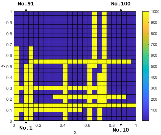
Fig.1 illustrates a sample of the permeability field, where the matrix permeability is 1 millidarcy, and the fracture permeability is 1000 millidarcy, with a total of 15 fractures present in the system. We define the coarse grid in the bottom left corner of the graph as No. 1 in coordinates that increase from left to right and from bottom to top. In this multi-scale system, the basis functions are defined on the coarse grid, but grids with different coordinates may have distinct basis functions even under the same permeability conditions (for instance, coarse grids No. 10 and No. 91 in Fig.1).
The initial permeability field was represented as a one-dimensional tensor. We reconstructed it into a two-dimensional tensor, where 100 and 9 correspond to the number of coarse grids and the number of fine grids within each coarse grid, respectively, while the structure of the basis function remained unchanged. This transformation enables the use of two-dimensional multi-scale convolutional filters for feature learning during the model construction. Considering that batch normalization was frequently applied within the model, data normalization was not performed during the preprocessing stage.
4 Methodology
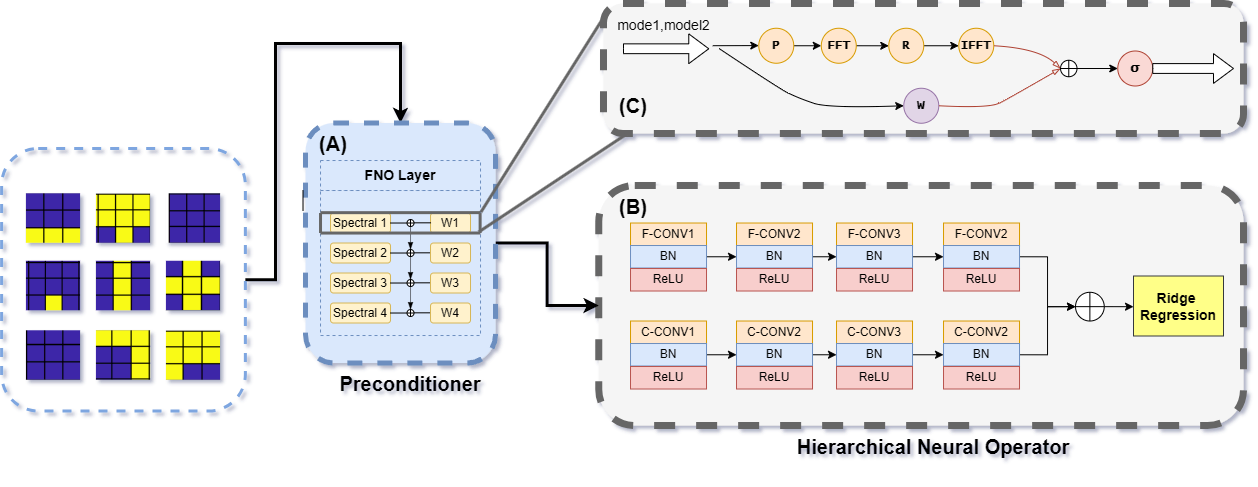
Our study proposed a Preconditioner-Learner architecture, combining the strengths of Fourier Neural Operator (FNO) and multi-scale neural network to learn basis functions. The FNO serves as a preconditioner, transforming the input into a spectral domain, where complex patterns can be learned more efficiently. This preconditioned input is then processed by a two-path multi-scale neural operator, which consists of convolutional layers that capture both coarse and fine-scale spatial features. Finally a Ridge regression layer with L2 regularization is employed to integrate the learned features and produce the final output.
4.1 Fourier Transformation-based Pre-conditioner
Fourier Neural Operator (FNO) is the first step of our model (Li et al.,2020; 2023), transforming the input into a richer representation in the frequency domain. The preconditioner applies the Fourier integral operator to convert into a spectral representation, which enables the model to capture local and global dependencies, giving a full understanding of the spatial relationships inherent in the basis functions. The Fourier integral operator is defined as
| (4) |
where is the Fourier transform of a periodic function parameterized by .
The operator plays a central role in converting the permeability field to the Fourier domain, thus achieving efficient spectral convolution. By learning the model adapts to different frequency component of the input, effectively capturing the global interaction. The Fourier transform is applied to the input function in the spatial domain, mapping it to the frequency domain:
| (5) |
where is the Fourier basis function and is the mesh sampled from the distribution . is the frequency mode. Assumed that is a periodic, square torus (Li et al.,2020) and the mesh is uniform, so the Fourier transform can be implemented by the 2-D fast Fourier transform (2D-FFT):
| (6) |
where is the computational domain.
In the frequency domain, the convolution operation is transformed into element-wise multiplications, which is efficient in computation:
| (7) |
where represents the learnable kernel in the Fourier domain, which allows the network to efficiently capture interactions across different spatial scales.
After performing spectral convolution so that learned weights perform the necessary operations in the frequency domain, the modified data is mapped back to the spatial domain using the inverse Fourier transform (IFFT):
| (8) |
This step enables the model to recover spatial patterns while taking advantage of spectral learning.
The process of the FNO layer reconstructs the input in the original domain and enrich the learning spectral information to capture global and non-global dependencies.
Our FNO-based preconditioner consists of multiple spectral convolution layers (here we set 4 layers). Fig.2-(A)(B) demonstrate the whole structure combining all the theories mentioned above, and convert the permeability from spatial domain to Fourier domain, then back to the spatial domain after pattern trimming. Each layer can capture different levels of frequency information. At each level, the input goes through the following process:
-
1.
Lifting and Fourier Transform: First Map the input to a higher dimension and transform from spatial domain to frequency domain using Fourier transform.
-
2.
Linear Transformation: Apply a linear transformation to the lower frequency modes while filtering out higher frequency models, which can be expressed as
(9) -
3.
Inverse Fourier Transform: Convert the data back to the spatial domain ().
-
4.
Pointwise Linear Transform, Combination and Activation: In parallel to the FFT, apply a local linear transformation to the original input . Combine the output from the frequency domain transformation and local transformation and passed through a non-linear activation function :
(10) (11) where , is the cumulative distribution function of standard normal distribution.
Go through the above process and follow the following iterative rules:
| (12) |
we can achieve the update of parameters in the Fourier Layer.
The preconditioner structure enables our model to operate on a feature space with more information while capturing both high and low frequency components of the input. It reduces the computational complexity from to , which can improve the convergence rate and achieve better performance when capturing complex spatial modes. This approach enables the model to adapt to various scales and boundary conditions.
4.2 Multi-scale Neural Operator for Basic Functions
Deep learning techniques have superior performance in constructing PDEs and basis function learners. A conventional convolutional neural network (CNN) consists of input, convolutional, pooling, fully connected, and output layers. The more complex the model has a larger order of parameters, which will put a certain demand on the computation and hardware. Compared with AlexNet (Krizhevsky et al.,2012) and VGGNet (Simonyan and Zisserman,2014), our multi-scale neural operater learner constructed in this study uses fewer layers, has less complexity, and can obtain ideal learning results in a lower training time.
Although the basis function we generated is defined on the coarse grid system, the fine grid system can still contain certain information. For this purpose, we employed convolutional filters at two different scales for information learning. Considering that a single-path neural network structure may alter feature scales, using convolutional kernels of two different scales within a single path could lead to the loss of some information.Hence, we have constructed a dual-path multi-scale convolutional neural operator architecture.
In this design, the output of the preconditioner is respectively passed through a large-scale net () and a small-scale net (), followed by feature fusion of the outputs from both paths, enabling multi-scale learning and hierarchical pattern learning. Since the size of filter used by small-scale CNN is , this path dose not change the specification and numerical results of data, then it can be regarded as a channel expansions operation of the initial information. This approach is pretty similar to the feature combination in FNO above and the physical information in Physical-informed Neural Networks (PINNs)(Raissi et al.,[23]), which enables maximum learning of the feature information contained in the multi-scale system.
In both the coarse grid path and fine grid path, the data output from the preprocessor is processed through a series of convolutional layers. A nonlinear mapping is performed in each convolutional layer:
| (13) |
where denotes the convolutional filters with kernel size or . represents batch normalization, and is the ReLU activation function. These layers capture spatial dependencies at both scales, effectively learning the multi-scale features of the input. Then this process will be flattened and passed to a fully connected layer. This layer implements Ridge regression using L2 regularization:
| (14) |
where denotes the learnable weights, and is the flattened feature map. The Ridge Regression loss function is given by:
| (15) |
where is the L2 regularization term, encouraging the model to maintain smaller weights, thereby improving generalization and preventing overfitting.
The multi-scale neural operator captures the hierarchical spatial structures in the data by learning both coarse-scale and fine-scale features through separate pathways, followed by channel fusion. Fig.2-(B) illustrates our multi-scale structure for learning multi-scale basis functions. This approach allows the model to adapt to details at different scales, thereby enhancing its ability to generalize to solutions of different basis functions.
The complete model integrates the spectral representation from the FNO preconditioner with the multi-scale convolutional features. This integration enables the model to capture both global (frequency-based) and local (spatial-based) dependencies, which is crucial for effectively modeling and solving basis function problems.
4.3 Ablation Study
Ablation study is an efficient method to investigate the superiority of the model and to evaluate the contribution of each component. In our study, to assess the effectiveness of the preconditioner and the advantage of the multi-scale neural operator compared to a single-scale learner, we conduct an ablation study by removing certain parts of the architecture to evaluate their impact on the learning of basis functions. To ensure experimental rigor, we adhere to the single-variable principle, where only one component (either the preconditioner, coarse-grid path, or fine-grid path) is removed at a time, while keeping all other components unchanged. The model is evaluated using the same metrics as the complete model, specifically MSE, MAE, and R2.
Removing the Preconditioner. The preconditioner is a crucial component of our proposed method. Removing this part causes the permeability field to be directly fed into the multi-scale operator for feature learning. To maintain structural consistency, we use a filter to process the data, ensuring that the output channel count matches that of the original preconditioner. All other structures and parameters, such as the number of training epochs and optimizer settings, remain unchanged.
Removing a Single-Scale Neural Operator. The multi-scale operator in our architecture learns features at different scales. To investigate the importance of different scales within the entire operator, we individually remove the coarse-grid path and fine-grid path. The primary impact of this modification on the structural design is that the output is directly fed into the fully connected layer without requiring convolutional fusion. For consistency, we continue using L2 regularization in the fully connected layer to simulate Ridge Regression. All other parameters and structures remain unchanged. The three models resulting from the different ablation methods are denoted as Ablation1 (Precondition), Ablation2 (Coarse), and Ablation3 (Fine), respectively. The specific experimental results will be presented and analyzed in the Results section.
4.4 Evaluation
The evaluation of the proposed model in our study is divided into three stages to comprehensively assess its performance, robustness, and generalization ability.
Model Evaluation. We use three standard metrics to evaluate the accuracy of the model’s learned basis functions: mean square error (MSE), mean absolute error (MAE), and coefficient of determination (R2).
MSE quantifies the average squared difference between predicted and actual values, offering insights into overall prediction accuracy and penalizing larger errors more severely.
| (16) |
MAE measures the average absolute difference between predictions and true values, providing a clearer indication of the model’s precision without over-penalizing outliers.
| (17) |
R2 represents the proportion of variance in the dependent variable that is explained by the independent variables, serving as an indicator of the model’s fit quality.
| (18) |
where , , denote the true value, predicted value and average of true value.
Subset Model MSE MAE R² Training Formal Ablation1 Ablation2 Ablation3 Validation Formal Ablation1 Ablation2 Ablation3 Testing Formal Ablation1 Ablation2 Ablation3 Total Formal Ablation1 Ablation2 Ablation3
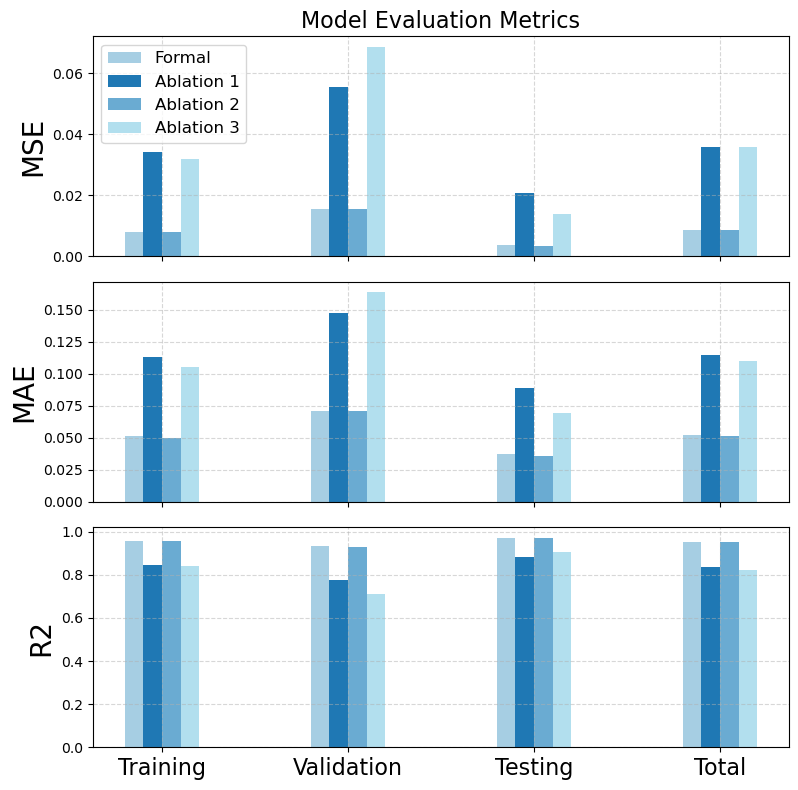
Robustness Assessment. To evaluate the model’s robustness and stability, we introduce perturbations into the input data and subsequently re-evaluate the model using the same three metrics: MSE, MAE, and R2. This approach allows us to observe how the model’s performance changes when exposed to noise, thereby assessing its resilience to data variability. A robust model is expected to demonstrate minimal variations in these metrics when subjected to such perturbations, indicating its stability under non-ideal conditions.
Generalization Ability. The model’s generalization ability is assessed using learning curves, which plot the training and validation errors against the number of training samples. By analyzing these curves, we can gain insights into whether the model is overfitting or underfitting. A well-generalized model will exhibit a decreasing gap between the training and validation errors as the training progresses, indicating its capability to perform consistently on unseen data.
This comprehensive evaluation framework ensures that the model’s accuracy, robustness, and ability to generalize to new data are rigorously tested, providing a solid foundation for its application in real-world scenarios.
5 Results
In this study, the performance of the model is described using both statistical analysis and visual representation. Tab.1 and Fig.5 present the evaluation results of the model and the ablation studies in two different ways. We will analyze the superiority of our model from several aspects.
The Impact of the Preconditioner on Model Performance. Ablation 1 represents the model without the preconditioner. As shown in Tab.1, the evaluation results indicate that the model’s MSE, MAE, and R2 on the testing set are 0.0206, 0.0887, and 0.8827, respectively, compared to 0.0036, 0.0602, and 0.9716 for the formal model. This comparison suggests that the preconditioner significantly enhances the learner’s ability to learn the basis functions. This architectural setup effectively improves the learning of features in the permeability field.
The Impact of Multi-scale Pathways on Model Performance. Ablation 2 and Ablation 3 represent ablation studies where the fine-grid system and coarse-grid system are removed, respectively. The evaluation metrics for Ablation 2 on the test set are 0.0035, 0.0357, and 0.9709 for MSE, MAE, and R2, while the corresponding metrics for Ablation 3 are 0.0357, 0.1098, and 0.8227. These results are consistent with the fact that the basis functions we learned are defined on the coarse-grid system. The exclusion of feature learning on the coarse grid has a significant impact on the overall model performance. Although the ablation of the fine-grid system did not result in a statistically significant decline in model performance, the fine-grid system still contains relevant information.
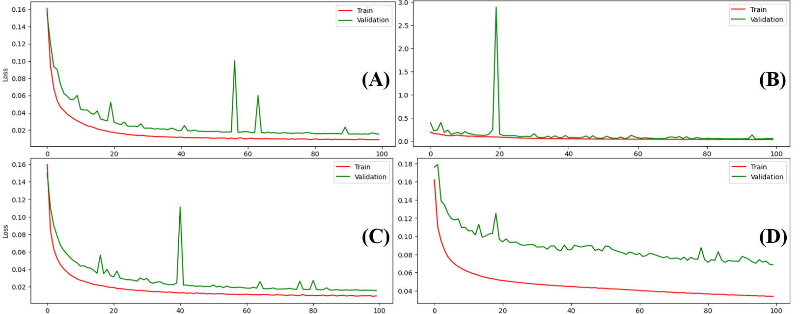
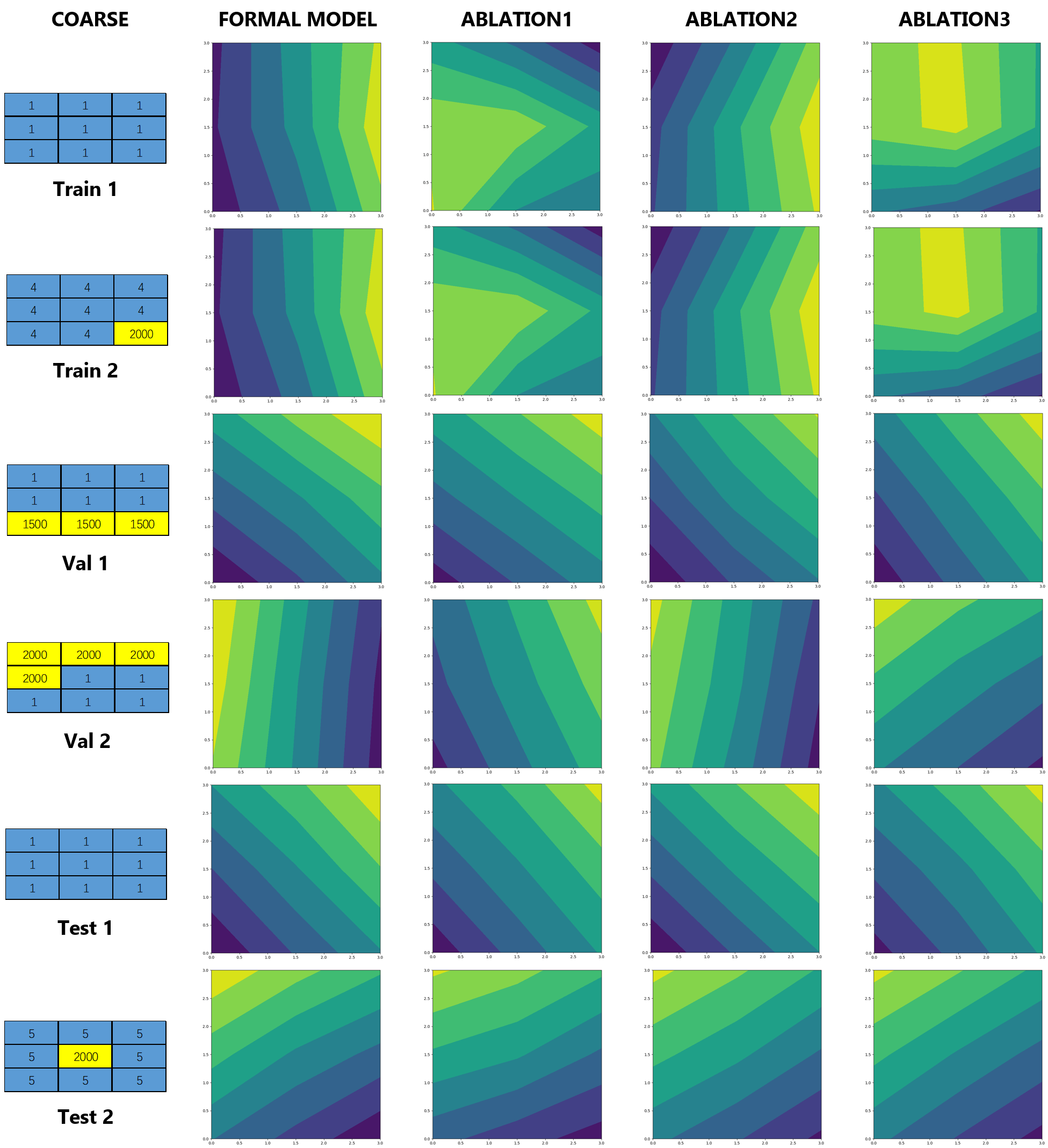
Fig.3 illustrates the reconstruction results of the model for the coarse-grid system. The left part displays a sample coarse grid from the simulated permeability fields, which were drawn from the training set, validation set, and testing set. In these grids, the blue regions represent matrix, the yellow regions indicate fractures, and the numbers in the grids denote the permeability at each location. The right part shows the reconstructions generated by different models. It is evident that the effectiveness of the preconditioner and the multi-scale learner can be observed from the reconstruction results. For homogenized permeability fields, the preconditioner demonstrates outstanding performance, aiding a single CNN model in extracting features more effectively.
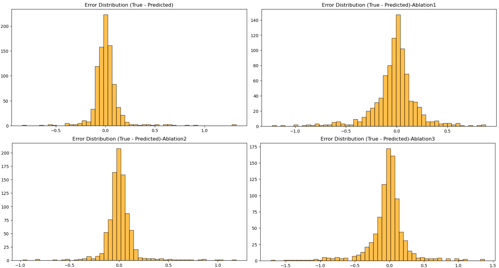
Additionally, we evaluate the model’s performance by observing the distribution of the errors (Fig.4). The concentration of errors can reflect model performance to a certain extent. We compared the learned basis functions with the original basis functions to calculate the errors, where models with error distributions centered around 0 exhibit superior performance. The results show that the model without the preconditioner displays a wider range of error values compared to other models. Furthermore, the error distribution of the model with the fine-grid system ablated closely resembles that of the complete model, indicating that the coarse-grid system contributes the majority of the information within the multi-scale system.
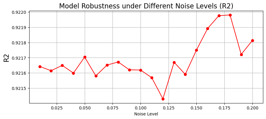
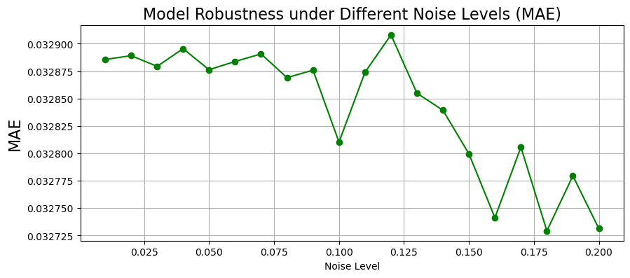
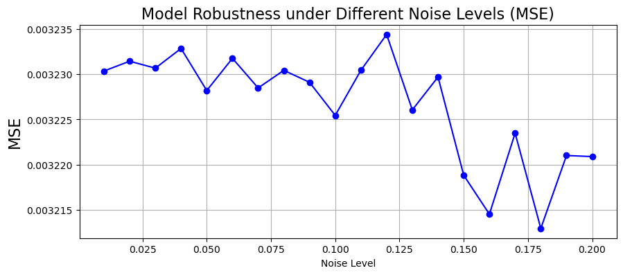
To evaluate the robustness of the model, we analyzed the variations in the evaluation metrics MSE, MAE, and R2 under the influence of 20 different levels of Gaussian noise ranging from 0.01 to 0.2. As shown in Fig.7, the MSE exhibits a fluctuating yet gradually decreasing trend with increasing noise levels, with changes consistently remaining within the range. Similarly, Fig.6 demonstrates that MAE experiences a fluctuating decline under different noise disturbances, also confined within the range, indicating that the model maintains high accuracy despite varying degrees of noise interference. In contrast, R2, as depicted in Fig.9, displays a fluctuating pattern and eventually rises as noise levels increase, with its overall change remaining within the magnitude. These findings indicate that the model exhibits robust performance under Gaussian noise interference, demonstrating an ability to resist noise and maintain stability and accuracy in predictions.
Fig.8 presents the learning curves of four models to evaluate their generalization capabilities. In Fig.8-(A), our proposed model demonstrates a consistent trend between training and validation losses, maintaining stability throughout the training process. The validation loss gradually decreases to a relatively low level, indicating that the model exhibits good fitting ability on both the training and validation sets, thereby demonstrating excellent generalization capability.
In contrast, the Ablation1 model shown in Fig.8-(B) (which excludes the preconditioner) exhibits a significant outlier in the validation loss, reaching as high as near to 3.0, indicating severe overfitting or instability on the validation set, thus reflecting poor generalization capability. The Ablation2 model in Fig.8-(C) (which excludes the fine grid pathway) and the Ablation3 model in Fig.8-(D) (which excludes the coarse grid pathway) both show some level of fluctuation in the validation loss. Although their fluctuations are not as dramatic as in Fig.8-(B), they are still higher overall compared to our proposed model.
These findings indicate that our proposed model (Fig.8-(A)) maintains stable performance across different datasets, with lower validation loss and no significant fluctuations, thereby proving its superior generalization capability in the presence of noise interference and model complexity.
6 Discussion
This study aims to develop a more accurate and efficient neural network architecture for learning multi-scale basis functions in porous media flow of subsurface fluids. By introducing a lightweight preconditioner-learner architecture, our proposed model demonstrated superior performance across evaluations of accuracy, generalization ability, and robustness, aligning well with our expectations.
The improved performance can be attributed to the preconditioner’s capability to transform data into the frequency (Fourier) domain, enabling the extraction of key features crucial for deep learning models. This suggests that preprocessing data before feeding it into convolutional neural network learners significantly enhances model learning efficacy. Additionally, we found that the multi-scale convolutional neural network effectively extracts features from different scales and incorporates them into the basis function learning, even when these functions are defined on a coarse grid system. This finding is further corroborated by our ablation study results, highlighting the critical role of the multi-scale structure in the model’s performance.
Compared to previous studies, our research aligns with established findings that deep learning techniques can be effectively applied for learning and reconstructing multi-scale basis functions with high accuracy. Importantly, the evaluation on the test set shows that our model achieved an MSE of 0.0036 and an R2 of 0.9716, while the corresponding results from the traditional convolutional neural network model of the previous research were 0.0466 and 0.8083, respectively(Choubineh et al.,2022). These outcomes clearly indicate that our model surpasses existing models in terms of accuracy. The introduction of the preconditioner and the multi-scale parallel learning strategy allowed our model to capture more features and effectively reconstruct the basis functions. Moreover, as observed from the learning curve (Fig.8), our model converges much faster, indicating that it requires less computational resources and training time compared to previous models, which is a significant advantage.
While these results are promising, there is significant potential to expand this work. One possible direction is to extend the current model to handle more complex three-dimensional permeability fields, which would enable a more comprehensive application in real-world subsurface environments. Additionally, the model could be adapted to handle multi-scale coupled systems that reflect the intricate interactions between different geological formations. Furthermore, evaluating the model’s performance using real reservoir data will be essential to validate its robustness and applicability in practical scenarios. Such enhancements would help in pushing the boundaries of subsurface fluid flow modeling and contribute to a more profound understanding of mineral exploration processes.
Despite these meaningful findings, certain limitations remain. The data used for training is relatively limited in scale compared to actual application environments, and only two scales were considered for model construction for simplicity, which might affect the model’s generalizability and application in more complex real-world scenarios. Nevertheless, the results of this study have significant implications for subsurface fluid flow and mineral exploration. Our model has the potential to reconstruct multi-scale basis functions based on actual permeability fields, providing valuable insights into subsurface mineral detection.
7 Conclusion
In this study, we presented FP-MsNet, a novel and efficient preconditioner-learner architecture for learning multi-scale basis functions in high-dimensional subsurface fluid flow. By integrating Fourier Neural Operator (FNO) with a multi-scale neural network architecture, our model effectively captures both global and local spatial features. Through comprehensive evaluations, FP-MsNet has demonstrated state-of-the-art (SOTA) performance, surpassing existing models in terms of accuracy, generalization, and robustness.
The ablation studies confirmed that the preconditioner and multi-scale pathways are critical components of our architecture, significantly contributing to its superior performance. Compared to traditional models, FP-MsNet achieved remarkably lower MSE, MAE and higher R2 scores, indicating its capability to capture complex spatial patterns with unprecedented precision.
Despite the promising results, limitations such as the relatively small training dataset and the simplicity of the two-scale model structure were acknowledged. Future work will focus on expanding the dataset and incorporating additional scales to enhance the model’s adaptability to more complex scenarios. Extending to three-dimensional data could further strengthen FP-MsNet’s applicability in real-world subsurface fluid flow modeling.
In summary, FP-MsNet represents the SOTA in multi-scale basis function reconstruction, offering a groundbreaking approach for subsurface fluid flow and mineral exploration, and establishing a robust foundation for future advancements in this field.
CRediT Authors Contributions Statement
Peiqi Li: Conceptualization, Methodology, Project administration, Visualization, Writing-original draft & review & editing. Jie Chen: Conceptualization, Data curation, Formal analysis, Methodology, Software, Supervision, Validation, Writing-review & editing.
Declaration of Competing Interests
The authors confirm that they have no conflicts of interest in regards to the content of this study.
Funding
This research did not receive any specific grant from funding agencies in the public, commercial, or not-for-profit sectors.
Acknowledgment
Thanks to Dr.Jie Chen for his support, resources and guidance during this study.
Data and Code Availability
Due to the proprietary considerations, both the dataset and the analysis code used in this study are not publicly available. Researchers interested in accessing the data or the code may contact the corresponding author for more information.
References
- Chen and Hou [2003] Z. Chen, T. Y. Hou, A mixed multiscale finite element method for elliptic problems with oscillating coefficients, Mathematics of Computation 72 (2003).
- Ganis et al. [2017] B. Ganis, D. Vassilev, C. Q. Wang, I. Yotov, A multiscale flux basis for mortar mixed discretizations of stokes-darcy flows, Computer Methods in Applied Mechanics & Engineering 313 (2017) 259–278.
- Jenny et al. [2005] P. Jenny, S. H. Lee, H. A. Tchelepi, Adaptive multiscale finite-volume method for multiphase flow and transport in porous media, Siam Journal on Multiscale Modeling & Simulation 3 (2005) 50–64.
- Hajibeygi et al. [2008] H. Hajibeygi, G. Bonfigli, M. A. Hesse, P. Jenny, Iterative multiscale finite-volume method, Journal of Computational Physics 227 (2008) 8604–8621.
- Azad et al. [2021] M.-R. Azad, A. Kamkar-Rouhani, B. Tokhmechi, M. Arashi, Hierarchical simultaneous upscaling of porosity and permeability features using the bandwidth of kernel function and wavelet transformation in two dimensions: Application to the spe-10 model, Oil & Gas Science and Technology–Revue d’IFP Energies nouvelles 76 (2021) 26.
- Efendiev et al. [2013] Y. Efendiev, J. Galvis, T. Y. Hou, Generalized multiscale finite element methods (gmsfem), Journal of computational physics 251 (2013) 116–135.
- Chen et al. [2020] J. Chen, E. T. Chung, Z. He, S. Sun, Generalized multiscale approximation of mixed finite elements with velocity elimination for subsurface flow, Journal of Computational Physics 404 (2020) 109133.
- Choubineh et al. [2022] A. Choubineh, J. Chen, F. Coenen, F. Ma, An innovative application of deep learning in multiscale modeling of subsurface fluid flow: Reconstructing the basis functions of the mixed gmsfem, Journal of Petroleum Science and Engineering 216 (2022) 110751.
- Choubineh et al. [2023] A. Choubineh, J. Chen, D. A. Wood, F. Coenen, F. Ma, Deep ensemble learning for high-dimensional subsurface fluid flow modeling, Engineering Applications of Artificial Intelligence 126 (2023) 106968.
- Geng et al. [2024] S. Geng, S. Zhai, C. Li, Swin transformer based transfer learning model for predicting porous media permeability from 2d images, Computers and Geotechnics 168 (2024) 106177.
- Meng et al. [2023] Y. Meng, J. Jiang, J. Wu, D. Wang, Transformer-based deep learning models for predicting permeability of porous media, Advances in Water Resources 179 (2023) 104520.
- Vaswani [2017] A. Vaswani, Attention is all you need, Advances in Neural Information Processing Systems (2017).
- Li et al. [2020] Z. Li, N. Kovachki, K. Azizzadenesheli, B. Liu, K. Bhattacharya, A. Stuart, A. Anandkumar, Fourier neural operator for parametric partial differential equations, arXiv preprint arXiv:2010.08895 (2020).
- Jenny et al. [2003] P. Jenny, S. Lee, H. A. Tchelepi, Multi-scale finite-volume method for elliptic problems in subsurface flow simulation, Journal of computational physics 187 (2003) 47–67.
- Hou and Wu [1997] T. Y. Hou, X.-H. Wu, A multiscale finite element method for elliptic problems in composite materials and porous media, Journal of computational physics 134 (1997) 169–189.
- Fu et al. [2024] S. Fu, E. Chung, L. Zhao, An efficient multiscale preconditioner for large-scale highly heterogeneous flow, SIAM Journal on Scientific Computing 46 (2024) S352–S377.
- Liu et al. [2024] X. Liu, B. Xu, S. Cao, L. Zhang, Mitigating spectral bias for the multiscale operator learning, Journal of Computational Physics 506 (2024) 112944.
- Fukunaga and Koontz [1970] K. Fukunaga, W. L. Koontz, Application of the karhunen-loeve expansion to feature selection and ordering, IEEE Transactions on computers 100 (1970) 311–318.
- Li et al. [2023] Z. Li, D. Z. Huang, B. Liu, A. Anandkumar, Fourier neural operator with learned deformations for pdes on general geometries, Journal of Machine Learning Research 24 (2023) 1–26.
- Li et al. [2020] Z. Li, N. Kovachki, K. Azizzadenesheli, B. Liu, K. Bhattacharya, A. Stuart, A. Anandkumar, Neural operator: Graph kernel network for partial differential equations, arXiv preprint arXiv:2003.03485 (2020).
- Krizhevsky et al. [2012] A. Krizhevsky, I. Sutskever, G. E. Hinton, Imagenet classification with deep convolutional neural networks, Advances in neural information processing systems 25 (2012).
- Simonyan and Zisserman [2014] K. Simonyan, A. Zisserman, Very deep convolutional networks for large-scale image recognition, arXiv preprint arXiv:1409.1556 (2014).
- Raissi et al. [2019] M. Raissi, P. Perdikaris, G. E. Karniadakis, Physics-informed neural networks: A deep learning framework for solving forward and inverse problems involving nonlinear partial differential equations, Journal of Computational physics 378 (2019) 686–707.