SUPPLEMENTARY MATERIAL TO: Fusion of Tree-induced Regressions for Clinico-genomic Data

Jeroen M. Goedhart^∗a, Mark A. van de Wiel^a, Wessel N. van Wieringen^a,b, Thomas Klausch^a

^∗Correspondence e-mail address: j.m.goedhart@amsterdamumc.nl

^aDepartment of Epidemiology and Data Science, Amsterdam Public Health Research Institute, Amsterdam University Medical Centers Location AMC, Meibergdreef 9, the Netherlands
^bDepartment of Mathematics, Vrije Universiteit, De Boelelaan 1081a, 1081 HV Amsterdam, The Netherlands

1 FusedTree for binary outcome

Recall that the fitted tree with $M$ leaf nodes induces data $\tilde{\boldsymbol{y}}\in\mathbb{R}^{N\times 1},$ $\tilde{\boldsymbol{X}}\in\mathbb{R}^{N\times Mp},$ and $\tilde{\boldsymbol{U}}\in\mathbb{R}^{N\times M}.$ We index observations, corresponding to the rows, of $\tilde{\boldsymbol{y}},$ $\tilde{\boldsymbol{X},}$ and $\tilde{\boldsymbol{U}}$ by $i,$ i.e. $\tilde{y}_{i},$ $\tilde{\boldsymbol{x}}_{i},$ and $\tilde{\boldsymbol{u}}_{i}$ . Then, for binary response $y_{i}\in\left\{0,1\right\},$ we consider the model

$$\tilde{y}_{i}\sim\textrm{Bernoulli}\left[\textrm{expit}\left(\tilde{\boldsymbol{u}}_{i}^{\top}\boldsymbol{c}+\tilde{\boldsymbol{x}}_{i}^{\top}\boldsymbol{\beta}\right)\right],\quad i=1,\ldots,N,$$ (1)

with again clinical intercept parameter vector $\boldsymbol{c}\in\mathbb{R}^{M},$ omics parameter vector $\boldsymbol{\beta}\in\mathbb{R}^{Mp},$ and $\textrm{expit$\left(x\right)$=}\exp\left(x\right)\left[1+\exp\left(x\right)\right]^{-1}.$ To find estimates $\hat{\boldsymbol{c}}$ of $\boldsymbol{c}$ and $\hat{\boldsymbol{\beta}}$ and $\boldsymbol{\beta},$ we solve

$$\hat{\boldsymbol{c}},\,\hat{\textbf{$\boldsymbol{\beta}$}} =\underset{\boldsymbol{c},\textbf{$\boldsymbol{\beta}$}}{\textrm{arg max}}\>\sum_{i=1}^{N}\tilde{y}_{i}\log\left[\textrm{expit}\left(\tilde{\boldsymbol{u}}_{i}^{\top}\boldsymbol{c}+\tilde{\boldsymbol{x}}_{i}^{\top}\boldsymbol{\beta}\right)\right]+\left(1-\tilde{y}_{i}\right)\log\left[1-\textrm{expit}\left(\tilde{\boldsymbol{u}}_{i}^{\top}\boldsymbol{c}+\tilde{\boldsymbol{x}}_{i}^{\top}\boldsymbol{\beta}\right)\right]$$

$$-\lambda\textbf{$\boldsymbol{\beta}$}^{T}\textbf{$\boldsymbol{\beta}$}-\alpha\textbf{$\boldsymbol{\beta}$}^{\top}\boldsymbol{\Omega}\textbf{$\boldsymbol{\beta}$}$$

$$=\underset{\boldsymbol{c},\textbf{$\boldsymbol{\beta}$}}{\textrm{arg max}}\>\sum_{i=1}^{N}\left\{\tilde{y}_{i}\left(\tilde{\boldsymbol{u}}_{i}^{\top}\boldsymbol{c}+\tilde{\boldsymbol{x}}_{i}^{\top}\boldsymbol{\beta}\right)-\log\left[1+\exp\left(\tilde{\boldsymbol{u}}_{i}^{\top}\boldsymbol{c}+\tilde{\boldsymbol{x}}_{i}^{\top}\boldsymbol{\beta}\right)\right]\right\}-\lambda\textbf{$\boldsymbol{\beta}$}^{T}\textbf{$\boldsymbol{\beta}$}-\alpha\textbf{$\boldsymbol{\beta}$}^{\top}\boldsymbol{\Omega}\textbf{$\boldsymbol{\beta}$},$$ (2)

i.e. optimizing the penalized log likelihood of all data for model (1).

Estimator (2) cannot be evaluated analytically and is hence found using the iterative re-weighted least squares (IRLS) algorithm.2

The IRLS algorithm updates estimates $\hat{\boldsymbol{c}}^{(t)},\,\hat{\textbf{$\boldsymbol{\beta}$}}^{(t)}\rightarrow\hat{\boldsymbol{c}}^{(t+1)},\,\hat{\textbf{$\boldsymbol{\beta}$}}^{(t+1)},$ with iteration index $t,$ until the estimates stabilize within some tolerance level. Specifically, define the linear predictor for the observations $\boldsymbol{\eta}^{(t)}=\left(\eta_{i}^{(t)}\right)_{i=1}^{N}\in\mathbb{R}^{N\times 1},$ with $\eta_{i}^{(t)}=\tilde{\boldsymbol{u}}_{i}^{\top}\hat{\boldsymbol{c}}^{(t)}+\tilde{\boldsymbol{x}}_{i}^{\top}\hat{\textbf{$\boldsymbol{\beta}$}}^{(t)}$, diagonal weight matrix $\boldsymbol{W}^{(t)}$ with $i$th element on the diagonal $W_{ii}^{(t)}=\exp\left(\eta_{i}^{(t)}\right)\left[\exp\left(\eta_{i}^{(t)}\right)+1\right]^{-2},$ Then, given current estimates $\hat{\boldsymbol{c}}^{(t)},\,\hat{\textbf{$\boldsymbol{\beta}$}}^{(t)},$ the updates equal:

$$\hat{\boldsymbol{c}}^{(t+1)} =\left\{\tilde{\boldsymbol{U}}^{\top}\left(\boldsymbol{W}^{(t)}\right)^{-1}\left[\textbf{$\tilde{\boldsymbol{X}}$}\left(\lambda\boldsymbol{I}_{Mp\times Mp}+\alpha\boldsymbol{\Omega}\right)^{-1}\textbf{$\tilde{\boldsymbol{X}}$}^{\top}+\left(\boldsymbol{W}^{(t)}\right)^{-1}\right]^{-1}\tilde{\boldsymbol{U}}\right\}^{-1}$$

$$\times\tilde{\boldsymbol{U}}^{\top}\left[\textbf{$\tilde{\boldsymbol{X}}$}\left(\lambda\boldsymbol{I}_{Mp\times Mp}+\alpha\boldsymbol{\Omega}\right)^{-1}\textbf{$\tilde{\boldsymbol{X}}$}^{\top}+\left(\boldsymbol{W}^{(t)}\right)^{-1}\right]^{-1}\left\{\boldsymbol{\eta}^{(t)}+\left(\boldsymbol{W}^{(t)}\right)^{-1}\left[\tilde{\boldsymbol{y}}-\textrm{expit}\left(\boldsymbol{\eta}^{(t)}\right)\right]\right\}$$

$$\hat{\textbf{$\boldsymbol{\beta}$}}^{(t+1)} =\left(\textbf{$\tilde{\boldsymbol{X}}$}^{\top}\boldsymbol{W}^{(t)}\textbf{$\tilde{\boldsymbol{X}}$}+\lambda\boldsymbol{I}_{Mp\times Mp}+\alpha\boldsymbol{\Omega}\right)^{-1}\textbf{$\tilde{\boldsymbol{X}}$}^{\top}\left[\boldsymbol{W}^{(t)}\left(\boldsymbol{\eta}^{(t)}-\tilde{\boldsymbol{U}}\hat{\boldsymbol{c}}^{(t+1)}\right)+\tilde{\boldsymbol{y}}-\textrm{expit}\left(\boldsymbol{\eta}^{(t)}\right)\right],$$ (3)

as was shown by Lettink et al. [2023]. We run the iterative algorithm until the penalized likelihood has stabilized within an absolute tolerance $\textrm{tol}=10^{-10}.$

2 FusedTree for survival outcome

For survival data, we have response $\tilde{y}_{i}=\left(t_{i},\delta_{i}\right)$ for observations $i=1,\ldots,N$ with $t_{i}$ the observed time at which patients had an event $\left(\delta_{i}=1\right)$ or were censored $\left(\delta_{i}=0\right).$ Again, we have tree-induced data $\tilde{\boldsymbol{X}}\in\mathbb{R}^{N\times Mp},$ and $\tilde{\boldsymbol{U}}\in\mathbb{R}^{N\times M}.$ We impose a proportional hazards model $h\left(t\mid X_{i}\right)=h_{0}\left(t\right)\exp\left(\tilde{\boldsymbol{u}}_{i}^{\top}\boldsymbol{c}+\tilde{\boldsymbol{x}}_{i}\boldsymbol{\beta}\right),$ which induces the penalized full log likelihood

$$l^{pen}\left(\boldsymbol{\beta},\boldsymbol{c},h_{0}\left(t\right);\tilde{\boldsymbol{y}},\tilde{\boldsymbol{X},}\tilde{\boldsymbol{U}}\right) =\sum_{i=1}^{N}\left\{-\exp\left(\tilde{\boldsymbol{u}}_{i}^{\top}\boldsymbol{c}+\tilde{\boldsymbol{x}}_{i}^{\top}\boldsymbol{\beta}\right)H_{0}(t_{i})+\delta_{i}\left[\log\left(h_{0}(t_{i})\right)+\tilde{\boldsymbol{u}}_{i}^{\top}\boldsymbol{c}+\tilde{\boldsymbol{x}}_{i}^{\top}\boldsymbol{\beta}\right]\right\}$$

$$-\lambda\textbf{$\boldsymbol{\beta}$}^{T}\textbf{$\boldsymbol{\beta}$}-\alpha\textbf{$\boldsymbol{\beta}$}^{\top}\boldsymbol{\Omega}\textbf{$\boldsymbol{\beta}$},$$ (4)

with baseline hazard $h_{0}\left(t\right)$ and cumulative baseline hazard $H_{0}\left(t\right)=\int_{t^{\prime}=0}^{t}h_{0}\left(t^{\prime}\right)dt^{\prime}.$ We then aim to find estimators $\hat{\boldsymbol{c}},\,\hat{\textbf{$\boldsymbol{\beta}$}}$ by

$$\hat{\boldsymbol{c}},\,\hat{\textbf{$\boldsymbol{\beta}$}}=\underset{\boldsymbol{c},\textbf{$\boldsymbol{\beta}$}}{\textrm{arg max}}\>l^{pen}\left(\boldsymbol{\beta},\boldsymbol{c},h_{0}\left(t\right);\tilde{\boldsymbol{y}},\tilde{\boldsymbol{X},}\tilde{\boldsymbol{U}}\right).$$ (5)

To solve (5), we use the iterative re-weighted least squares (IRLS) algorithm proposed by van Houwelingen et al. [2006]. Conveniently, this algorithm is almost identical to the IRLS algorithm for logistic regression, i.e. (3), as shown by van de Wiel et al. [2021]. The only differences between logistic regression and penalized cox regression are weights $W_{ii}^{(t)},$ which for penalized cox regression become $W_{ii}^{(t)}=\hat{H}_{0}^{(t)}\left(t\right)\exp\left(\tilde{\boldsymbol{u}}_{i}^{\top}\hat{\boldsymbol{c}}^{(t)}+\tilde{\boldsymbol{x}}_{i}^{\top}\hat{\textbf{$\boldsymbol{\beta}$}}^{(t)}\right),$ and centered response $\tilde{\boldsymbol{y}}-\textrm{expit}\left(\boldsymbol{\eta}^{(t)}\right),$ which equals $\tilde{\boldsymbol{y}}-\textrm{diag}\left(\boldsymbol{W}^{(t)}\right)$ for penalized cox regression. These changes are plugged into (3) and we run the iterative algorithm until penalized likelihood (4) has stabilized within an absolute tolerance $\textrm{tol}=10^{-10}$.

For iterative estimates $\hat{H}_{0}^{(t)}\left(t\right)$ of baseline hazard $H_{0}\left(t\right),$ we employ the Breslow estimator: $\hat{H}_{0}^{(t)}\left(t\right)=\sum_{i:\,t_{i}\leq t}\left\{\delta_{i}\left[\sum_{j:\,t_{j}\geq t_{i}}\exp\left(\tilde{\boldsymbol{u}}_{i}^{\top}\hat{\boldsymbol{c}}^{(t-1)}+\tilde{\boldsymbol{x}}_{i}^{\top}\hat{\textbf{$\boldsymbol{\beta}$}}^{(t-1)}\right)\right]^{-1}\right\}.$

3 Hyper-parameter tuning

To tune hyperparameters $\alpha$ and $\lambda,$ we solve for continuous response:

$$\hat{\lambda},\,\hat{\alpha}=\underset{\lambda,\,\alpha}{\textrm{arg min}}\frac{1}{K}\sum_{k=1}^{K}\left\|\tilde{\boldsymbol{y}}_{\varGamma_{k}}-\tilde{\boldsymbol{U}}_{\varGamma_{k}}\hat{\boldsymbol{c}}_{-\varGamma_{k}}\left(\lambda,\alpha\right)-\textbf{$\tilde{\boldsymbol{X}}$}_{\varGamma_{k}}\textbf{$\hat{\boldsymbol{\beta}}$}_{-\varGamma_{k}}\left(\lambda,\alpha\right)\right\|_{2}^{2},\quad\textrm{subject to}\quad\lambda,\,\alpha>0,$$ (6)

and for binary response, we solve:

$$\hat{\lambda},\,\hat{\alpha} =\underset{\lambda,\,\alpha}{\textrm{arg min}}\frac{1}{K}\sum_{k=1}^{K}\left\{\sum_{i\in\varGamma_{k}}\tilde{y}_{i}\left(\tilde{\boldsymbol{u}}_{i}\hat{\boldsymbol{c}}_{-\varGamma_{k}}\left(\lambda,\alpha\right)+\tilde{\boldsymbol{x}}_{i}^{\top}\textbf{$\hat{\boldsymbol{\beta}}$}_{-\varGamma_{k}}\left(\lambda,\alpha\right)\right)\right\}$$

$$-\frac{1}{K}\sum_{k=1}^{K}\left\{\sum_{i\in\varGamma_{k}}\log\left[1+\exp\left(\tilde{\boldsymbol{u}}_{i}^{\top}\hat{\boldsymbol{c}}_{-\varGamma_{k}}\left(\lambda,\alpha\right)+\tilde{\boldsymbol{x}}_{i}^{\top}\textbf{$\hat{\boldsymbol{\beta}}$}_{-\varGamma_{k}}\left(\lambda,\alpha\right)\right)\right]\right\}$$

$$\quad\textrm{subject to}\quad\lambda,\,\alpha>0,$$ (7)

and for survival response, we solve:

$$\hat{\lambda},\,\hat{\alpha}=\underset{\lambda,\,\alpha}{\textrm{arg min}} \frac{1}{K}\sum_{k=1}^{K}\left\{\sum_{i\in\varGamma_{k}}-\exp\left(\tilde{\boldsymbol{u}}_{i}^{\top}\hat{\boldsymbol{c}}_{-\varGamma_{k}}\left(\lambda,\alpha\right)+\tilde{\boldsymbol{x}}_{i}^{\top}\textbf{$\hat{\boldsymbol{\beta}}$}_{-\varGamma_{k}}\left(\lambda,\alpha\right)\right)\hat{H}_{0}(t_{i})\right\}$$

$$+\frac{1}{K}\sum_{k=1}^{K}\left\{\sum_{i\in\varGamma_{k}}\delta_{i}\left[\log\left(\hat{h}{}_{0}(t_{i})\right)+\tilde{\boldsymbol{u}}_{i}^{\top}\hat{\boldsymbol{c}}_{-\varGamma_{k}}\left(\lambda,\alpha\right)+\tilde{\boldsymbol{x}}_{i}^{\top}\textbf{$\hat{\boldsymbol{\beta}}$}_{-\varGamma_{k}}\left(\lambda,\alpha\right)\right]\right\}$$ (8)

$$\quad\textrm{subject to}\quad\lambda,\,\alpha>0,$$

with $\varGamma_{k}$ the observations in test fold $K$ and $-\varGamma_{k}$ the remaining samples forming the training set. Thus, we select $\hat{\lambda},\,\hat{\alpha}$ by minimizing the cross-validated prediction mean square error for continuous $\tilde{y}_{i}$ and the cross-validated likelihood for binary and survival $\tilde{y}_{i}.$

The above optimizations depend on repeated evaluation of estimators $\hat{\boldsymbol{c}}_{-\varGamma_{k}}\left(\lambda,\alpha\right)$ and $\textbf{$\hat{\boldsymbol{\beta}}$}_{-\varGamma_{k}}\left(\lambda,\alpha\right),$ which requires considerable computational time for high-dimensional data. As was shown by van de Wiel et al. [2021], a computationally more efficient procedure is to directly evaluate the linear predictors $\tilde{\boldsymbol{U}}_{\varGamma_{k}}\hat{\boldsymbol{c}}_{-\varGamma_{k}}\left(\lambda,\alpha\right)$ and $\textbf{$\tilde{\boldsymbol{X}}$}_{\varGamma_{k}}\textbf{$\hat{\boldsymbol{\beta}}$}_{-\varGamma_{k}}\left(\lambda,\alpha\right),$ i.e. the estimators in combination with their corresponding design matrices. These linear predictors can be reformulated such that their evaluation only requires repeated operations on matrices of dimension $N-\left|\varGamma_{k}\right|$ instead of dimension $Mp$ for evaluation of $\hat{\boldsymbol{c}}_{-\varGamma_{k}}\left(\lambda,\alpha\right)$ and $\textbf{$\hat{\boldsymbol{\beta}}$}_{-\varGamma_{k}}\left(\lambda,\alpha\right).$ The linear predictors are given, as derived by Lettink et al. [2023], with $\check{\boldsymbol{X}}=\tilde{\boldsymbol{X}}\boldsymbol{V}_{\varOmega}\left(\lambda\boldsymbol{I}_{p\times p}+\alpha\boldsymbol{D}_{\varOmega}\right)^{-\frac{1}{2}},$ by

$$\tilde{\boldsymbol{U}}_{\varGamma_{k}}\hat{\boldsymbol{c}}_{-\varGamma_{k}}\left(\lambda,\alpha\right) =\tilde{\boldsymbol{U}}_{\varGamma_{k}}\left[\tilde{\boldsymbol{U}}_{-\varGamma_{k}}^{\top}\left(\check{\boldsymbol{X}}_{-\varGamma_{k}}\check{\boldsymbol{X}}_{-\varGamma_{k}}^{\top}+\boldsymbol{I}_{\left|-\varGamma_{k}\right|\times\left|-\varGamma_{k}\right|}\right)^{-1}\tilde{\boldsymbol{U}}_{-\varGamma_{k}}\right]^{-1}$$

$$\times\tilde{\boldsymbol{U}}_{-\varGamma_{k}}^{\top}\left(\check{\boldsymbol{X}}_{-\varGamma_{k}}\check{\boldsymbol{X}}_{-\varGamma_{k}}^{\top}+\boldsymbol{I}_{\left|-\varGamma_{k}\right|\times\left|-\varGamma_{k}\right|}\right)^{-1}\tilde{\boldsymbol{y}}_{-\varGamma_{k}}$$

$$\textbf{$\tilde{\boldsymbol{X}}$}_{\varGamma_{k}}\textbf{$\hat{\boldsymbol{\beta}}$}_{-\varGamma_{k}}\left(\lambda,\alpha\right) =\check{\boldsymbol{X}}_{\varGamma_{k}}\check{\boldsymbol{X}}_{-\varGamma_{k}}^{\top}\left(\check{\boldsymbol{X}}_{-\varGamma_{k}}\check{\boldsymbol{X}}_{-\varGamma_{k}}^{\top}+\boldsymbol{I}_{\left|-\varGamma_{k}\right|\times\left|-\varGamma_{k}\right|}\right)^{-1}\left(\tilde{\boldsymbol{y}}_{-\varGamma_{k}}-\tilde{\boldsymbol{U}}_{-\varGamma_{k}}\hat{\boldsymbol{c}}_{-\varGamma_{k}}\right),$$

for continuous response, and

$$\tilde{\boldsymbol{U}}_{\varGamma_{k}}\hat{\boldsymbol{c}}_{-\varGamma_{k}}^{(t+1)}\left(\lambda,\alpha\right) =\tilde{\boldsymbol{U}}_{\varGamma_{k}}\left\{\tilde{\boldsymbol{U}}_{-\varGamma_{k}}^{\top}\left(\boldsymbol{W}_{-\varGamma_{k},-\varGamma_{k}}^{(t)}\right)^{-1}\left[\check{\boldsymbol{X}}_{-\varGamma_{k}}\check{\boldsymbol{X}}_{-\varGamma_{k}}^{\top}+\left(\boldsymbol{W}_{-\varGamma_{k},-\varGamma_{k}}^{(t)}\right)^{-1}\right]^{-1}\tilde{\boldsymbol{U}}_{-\varGamma_{k}}\right\}^{-1}$$

$$\times\tilde{\boldsymbol{U}}_{-\varGamma_{k}}^{\top}\left[\check{\boldsymbol{X}}_{-\varGamma_{k}}\check{\boldsymbol{X}}_{-\varGamma_{k}}^{\top}+\left(\boldsymbol{W}_{-\varGamma_{k},-\varGamma_{k}}^{(t)}\right)^{-1}\right]^{-1}\left\{\boldsymbol{\eta}_{-\varGamma_{k}}^{(t)}+\left(\boldsymbol{W}_{-\varGamma_{k},-\varGamma_{k}}^{(t)}\right)^{-1}\right.$$

$$\left.\times\left[\tilde{\boldsymbol{y}}_{-\varGamma_{k}}-\textrm{expit}\left(\boldsymbol{\eta}_{-\varGamma_{k}}^{(t)}\right)\right]\right\}$$

$$\textbf{$\tilde{\boldsymbol{X}}$}_{\varGamma_{k}}\textbf{$\hat{\boldsymbol{\beta}}$}_{-\varGamma_{k}}^{(t+1)}\left(\lambda,\alpha\right) =\check{\boldsymbol{X}}_{\varGamma_{k}}\check{\boldsymbol{X}}_{-\varGamma_{k}}^{\top}\left[\check{\boldsymbol{X}}_{-\varGamma_{k}}\check{\boldsymbol{X}}_{-\varGamma_{k}}^{\top}+\left(\boldsymbol{W}_{-\varGamma_{k},-\varGamma_{k}}^{(t)}\right)^{-1}\right]^{-1}$$

$$\times\left\{\boldsymbol{\eta}_{-\varGamma_{k}}^{(t)}-\tilde{\boldsymbol{U}}_{-\varGamma_{k}}\hat{\boldsymbol{c}}_{-\varGamma_{k}}^{(t+1)}+\left(\boldsymbol{W}_{-\varGamma_{k},-\varGamma_{k}}^{(t)}\right)^{-1}\left[\tilde{\boldsymbol{y}}_{-\varGamma_{k}}-\textrm{expit}\left(\boldsymbol{\eta}_{-\varGamma_{k}}^{(t)}\right)\right]\right\},$$

for binary response, with diagonal weight matrix $W_{-\varGamma_{k},-\varGamma_{k}}^{(t)}$ and linear predictor $\boldsymbol{\eta}_{-\varGamma_{k}}^{(t)}$ defined as in Appendix 1 combined with appropriate subsetting. Again, for survival response, we use a similar algorithm as for binary response in which only weights $W_{-\varGamma_{k},-\varGamma_{k}}^{(t)}$ and $\tilde{\boldsymbol{y}}_{-\varGamma_{k}}-\textrm{expit}\left(\boldsymbol{\eta}_{-\varGamma_{k}}^{(t)}\right)$ are modified as described in Appendix 2 .

Optimizations 6 and 7 are performed using the Nelder-Mead method (Nelder and Mead, 1965) implemented in the base R optim function with penalties $\lambda,\alpha$ on the $\log$-scale.

4 Shrinkage limits

Here, we derive the shrinkage limits of the FusedTree estimator, which we presented in eq. 6 of the main text.

Define $\boldsymbol{\varLambda}_{\lambda,\alpha}=\lambda\boldsymbol{I}_{Mp\times Mp}+\alpha\boldsymbol{\Omega},$ and recall $\boldsymbol{\Omega}=\boldsymbol{I}_{p\times p}\bigotimes\left(\boldsymbol{I}_{M\times M}-\frac{1}{M}\boldsymbol{1}_{M\times M}\right),$ with $M$ the number of leaf nodes. The estimators for the tree-induced clinical effect $\boldsymbol{c}$ and omics effects $\boldsymbol{\beta}$ are

$$\hat{\boldsymbol{c}} =\left\{\tilde{\boldsymbol{U}}^{\top}\left[\textbf{$\tilde{\boldsymbol{X}}$}\boldsymbol{\varLambda}_{\lambda,\alpha}^{-1}\textbf{$\tilde{\boldsymbol{X}}$}^{\top}+\boldsymbol{I}_{N\times N}\right]^{-1}\tilde{\boldsymbol{U}}\right\}^{-1}$$

$$\times\tilde{\boldsymbol{U}}^{\top}\left[\textbf{$\tilde{\boldsymbol{X}}$}\boldsymbol{\varLambda}_{\lambda,\alpha}^{-1}\textbf{$\tilde{\boldsymbol{X}}$}^{\top}+\boldsymbol{I}_{N\times N}\right]^{-1}\tilde{\boldsymbol{y}}$$

$$\hat{\textbf{$\boldsymbol{\beta}$}} =\left(\textbf{$\tilde{\boldsymbol{X}}$}^{\top}\textbf{$\tilde{\boldsymbol{X}}$}+\boldsymbol{\varLambda}_{\lambda,\alpha}\right)^{-1}\textbf{$\tilde{\boldsymbol{X}}$}^{\top}\left(\tilde{\boldsymbol{y}}-\tilde{\boldsymbol{U}}\hat{\boldsymbol{c}}\right),$$

$$=\left[\boldsymbol{\varLambda}_{\lambda,\alpha}^{-1}-\boldsymbol{\varLambda}_{\lambda,\alpha}^{-1}\textbf{$\tilde{\boldsymbol{X}}$}^{\top}\left(\textbf{$\tilde{\boldsymbol{X}}$}\boldsymbol{\varLambda}_{\lambda,\alpha}^{-1}\textbf{$\tilde{\boldsymbol{X}}$}^{\top}+\boldsymbol{I}_{N\times N}\right)^{-1}\textbf{$\tilde{\boldsymbol{X}}$}\boldsymbol{\varLambda}_{\lambda,\alpha}^{-1}\right]\textbf{$\tilde{\boldsymbol{X}}$}^{\top}\left(\tilde{\boldsymbol{y}}-\tilde{\boldsymbol{U}}\hat{\boldsymbol{c}}\right)$$ (9)

with the last line of (9) following from Woodbury’s identity. To derive the shrinkage limits ($\lambda\rightarrow\infty$ and $\alpha\rightarrow\infty$) of (9), we first find $\boldsymbol{\varLambda}_{\lambda,\alpha}^{-1}.$ Because $\boldsymbol{\varLambda}_{\lambda,\alpha}=\boldsymbol{I}_{p\times p}\bigotimes\boldsymbol{A},$ with $A=(\lambda+\alpha)\boldsymbol{I}_{M\times M}-\frac{\alpha}{M}\boldsymbol{1}_{M\times M},$ we have $\boldsymbol{\varLambda}_{\lambda,\alpha}^{-1}=\boldsymbol{I}_{p\times p}\bigotimes\boldsymbol{A}^{-1},$ and we are left with determining $\boldsymbol{A}^{-1},$ which can be shown to equal

$$\boldsymbol{A}^{-1}=\begin{pmatrix}a&b&\cdots&b\\ b&\ddots&\ddots&\vdots\\ \vdots&\ddots&a&b\\ b&\cdots&b&a\end{pmatrix}\in\mathbb{R}^{M\times M},$$

having identical diagonal elements $a=\lambda^{-1}-\alpha\left(1-1/M\right)\left(\lambda^{2}+\lambda\alpha\right)^{-1}$ and identical off-diagonal elements $b=\alpha\left(\lambda^{2}M+\lambda\alpha M\right)^{-1}.$ For $\lambda\rightarrow\infty,$ we have $a=b=0,$ and for $\alpha\rightarrow\infty,$ we have $a=b=1/\left(\lambda M\right).$ Thus, we have

$$\lim_{\lambda\rightarrow\infty}\boldsymbol{\varLambda}_{\lambda,\alpha}^{-1} =\boldsymbol{0}_{Mp\times Mp}$$ (10)

$$\lim_{\alpha\rightarrow\infty}\boldsymbol{\varLambda}_{\lambda,\alpha}^{-1} =\frac{1}{\lambda M}\boldsymbol{I}_{p\times p}\bigotimes\boldsymbol{1}_{M\times M}.$$ (11)

Limit (10) renders estimators$\boldsymbol{:}$

$$\lim_{\lambda\rightarrow\infty}\hat{\boldsymbol{c}} =\left(\tilde{\boldsymbol{U}}^{\top}\tilde{\boldsymbol{U}}\right)^{-1}\tilde{\boldsymbol{U}}^{\top}\tilde{\boldsymbol{y}}$$ (12)

$$\lim_{\lambda\rightarrow\infty}\hat{\textbf{$\boldsymbol{\beta}$}} =\boldsymbol{0}_{Mp},$$

with the first line the standard normal equation, as expected.

For $\alpha\rightarrow\infty,$ we first define the face-splitting product (Slyusar, 1999) by $\bullet,$ with matrix $\boldsymbol{C}=\boldsymbol{A}\bullet\boldsymbol{B}$ having row $i$ defined by the Kronecker product of corresponding rows $i$ of $\boldsymbol{A}$ and $\boldsymbol{B}.$ For $\boldsymbol{A}\in\mathbb{R}^{N\times M}$ and $\boldsymbol{B}\in\mathbb{R}^{N\times p},$ we then have $\boldsymbol{C}\in\mathbb{R}^{N\times Mp}.$ We also define the column-wise Kronecker product, i.e. the the Khatri–Rao product (Khatri and Rao, 1968), by $\ast,$ with $\boldsymbol{C}=\boldsymbol{A}\ast\boldsymbol{B}$ having column $j$ defined by the Kronecker product of column $j$ of $\boldsymbol{A}$ and $\boldsymbol{B}.$ For these products, the following useful properties hold (Slyusar, 1999):

$$\left(\boldsymbol{A}\bullet\boldsymbol{B}\right)\left(\boldsymbol{C}\bigotimes\boldsymbol{D}\right) =\left(\boldsymbol{AC}\right)\bullet\left(\boldsymbol{BD}\right)$$

$$\left(\boldsymbol{A}\bigotimes\boldsymbol{B}\right)\left(\boldsymbol{C}\ast\boldsymbol{D}\right) =\left(\boldsymbol{AC}\right)\ast\left(\boldsymbol{BD}\right)$$

$$\left(\boldsymbol{A}\bullet\boldsymbol{B}\right)\left(\boldsymbol{C}\ast\boldsymbol{D}\right) =\left(\boldsymbol{AC}\right)\circ\left(\boldsymbol{BD}\right)$$

$$\left(\boldsymbol{A}\bullet\boldsymbol{B}\right)^{\top} =\boldsymbol{A}^{\top}\ast\boldsymbol{B}^{\top}$$

with $\circ$ the Hadamard product, and all matrices of the right dimension to perform multiplication. These definitions are useful because we may define the tree-induced omics matrix $\tilde{\boldsymbol{X}}$ by

$$\tilde{\boldsymbol{X}}=\boldsymbol{X}\bullet\tilde{\boldsymbol{U}},$$ (13)

with $\boldsymbol{X}\in\mathbb{R}^{N\times p}$ the original omics covariate matrix.

We start with $\underset{\alpha\rightarrow\infty}{\lim}\hat{\boldsymbol{c}}.$ The limit $\underset{\alpha\rightarrow\infty}{\lim}\left[\textbf{$\tilde{\boldsymbol{X}}$}\boldsymbol{\varLambda}_{\lambda,\alpha}^{-1}\textbf{$\tilde{\boldsymbol{X}}$}^{\top}+\boldsymbol{I}_{N\times N}\right]^{-1}$ in (9) is simplified using (13) to

$$\lim_{\alpha\rightarrow\infty}\textbf{$\tilde{\boldsymbol{X}}$}\boldsymbol{\varLambda}_{\lambda,\alpha}^{-1}\textbf{$\tilde{\boldsymbol{X}}$}^{\top} =\frac{1}{\lambda M}\textbf{$\left(\boldsymbol{X}\bullet\tilde{\boldsymbol{U}}\right)$}\left(\boldsymbol{I}_{p\times p}\bigotimes\boldsymbol{1}_{M\times M}\right)\textbf{$\left(\boldsymbol{X}\bullet\tilde{\boldsymbol{U}}\right)$}^{\top}$$

$$=\frac{1}{\lambda M}\textbf{$\left(\boldsymbol{X}\bullet\tilde{\boldsymbol{U}}\boldsymbol{1}_{M\times M}\right)$}\textbf{$\left(\boldsymbol{X}^{\top}\ast\tilde{\boldsymbol{U}}^{\top}\right)$}$$

$$=\frac{1}{\lambda M}\textbf{$\left(\boldsymbol{X}\boldsymbol{X}^{\top}\right)$}\circ\left(\tilde{\boldsymbol{U}}\boldsymbol{1}_{M\times M}\tilde{\boldsymbol{U}}^{\top}\right)=\frac{1}{\lambda M}\textbf{$\boldsymbol{X}\boldsymbol{X}^{\top}$},$$ (14)

where we used $\tilde{\boldsymbol{U}}\boldsymbol{1}_{M\times M}\tilde{\boldsymbol{U}}^{\top}=\boldsymbol{1}_{N\times N}.$ This leads to the following limit

$$\lim_{\alpha\rightarrow\infty}\hat{\boldsymbol{c}} =\left\{\tilde{\boldsymbol{U}}^{\top}\left[\boldsymbol{X}\left(\frac{1}{\lambda M}\boldsymbol{I}_{p\times p}\right)\boldsymbol{X}^{\top}+\boldsymbol{I}_{N\times N}\right]^{-1}\tilde{\boldsymbol{U}}\right\}^{-1}$$

$$\times\tilde{\boldsymbol{U}}^{\top}\left[\boldsymbol{X}\left(\frac{1}{\lambda M}\boldsymbol{I}_{p\times p}\right)\boldsymbol{X}^{\top}+\boldsymbol{I}_{N\times N}\right]^{-1}\tilde{\boldsymbol{y}}.$$ (15)

Equation (15) is almost identical to the unpenalized effect estimator of a standard ridge regression with unpenalized $\tilde{\boldsymbol{U}}$ and penalized $\boldsymbol{X}$ (so the limit $\underset{\alpha\rightarrow\infty}{\lim}$ reduces $\tilde{\boldsymbol{X}}$ to $\boldsymbol{X}$). The standard ridge penalty, however, is multiplied by $M$ in (15) to account for having a factor $M$ more omics effect estimates.

Next, we compute $\underset{\alpha\rightarrow\infty}{\lim}\hat{\boldsymbol{\beta}}.$ We first note the equality

$$\lim_{\alpha\rightarrow\infty}\boldsymbol{\varLambda}_{\lambda,\alpha}^{-1}\textbf{$\tilde{\boldsymbol{X}}$}^{\top}=\frac{1}{\lambda M}\left(\boldsymbol{I}_{p\times p}\bigotimes\boldsymbol{1}_{M\times M}\right)\textbf{$\left(\boldsymbol{X}^{\top}\ast\tilde{\boldsymbol{U}}^{\top}\right)$}=\frac{1}{\lambda M}\boldsymbol{X}^{\top}\ast\boldsymbol{1}_{M\times N}.$$ (16)

Then, plugging (14) and (16) into the last line of (9) renders

$$\underset{\alpha\rightarrow\infty}{\lim}\hat{\boldsymbol{\beta}} =\left[\frac{1}{\lambda M}\boldsymbol{X}^{\top}\ast\boldsymbol{1}_{M\times N}-\frac{1}{\lambda M}\boldsymbol{X}^{\top}\ast\boldsymbol{1}_{M\times N}\left(\boldsymbol{I}_{N\times N}+\frac{1}{\lambda M}\textbf{$\boldsymbol{X}\boldsymbol{X}^{\top}$}\right)^{-1}\frac{1}{\lambda M}\textbf{$\boldsymbol{X}\boldsymbol{X}^{\top}$}\right]\left(\tilde{\boldsymbol{y}}-\tilde{\boldsymbol{U}}\hat{\boldsymbol{c}}\right)$$

$$=\left[\frac{1}{\lambda M}\boldsymbol{X}^{\top}-\frac{1}{\left(\lambda M\right)^{2}}\boldsymbol{X}^{\top}\left(\boldsymbol{I}_{N\times N}+\frac{1}{\lambda M}\textbf{$\boldsymbol{X}\boldsymbol{X}^{\top}$}\right)^{-1}\textbf{$\boldsymbol{X}\boldsymbol{X}^{\top}$}\right]\ast\boldsymbol{1}_{M\times N}\left(\tilde{\boldsymbol{y}}-\tilde{\boldsymbol{U}}\hat{\boldsymbol{c}}\right)$$

$$=\left\{\left[\frac{1}{\lambda M}\boldsymbol{I}_{N\times N}-\frac{1}{\left(\lambda M\right)^{2}}\boldsymbol{X}^{\top}\left(\boldsymbol{I}_{N\times N}+\frac{1}{\lambda M}\textbf{$\boldsymbol{X}\boldsymbol{X}^{\top}$}\right)^{-1}\textbf{$\boldsymbol{X}$}\right]\boldsymbol{X}^{\top}\ast\boldsymbol{1}_{M\times N}\right\}\left(\tilde{\boldsymbol{y}}-\tilde{\boldsymbol{U}}\hat{\boldsymbol{c}}\right),$$

with the second line following from the associativity of the Khatri-Rhao product: $\boldsymbol{A}\ast\boldsymbol{1}_{M\times N}+\boldsymbol{B}\ast\boldsymbol{1}_{M\times N}=\left(\boldsymbol{A}+\boldsymbol{B}\right)\ast\boldsymbol{1}_{M\times N},$ and because $\left(\boldsymbol{A}\ast\boldsymbol{1}_{M\times N}\right)\boldsymbol{B}=\left(\boldsymbol{AB}\right)\ast\boldsymbol{1}_{M\times N}.$ In the last line, we pulled out $\boldsymbol{X}^{\top}$ at the right-hand side of the $\left[\right]$ brackets. We then recognize the Woodbury identity

$$\frac{1}{\lambda M}\boldsymbol{I}_{N\times N}-\frac{1}{\left(\lambda M\right)^{2}}\boldsymbol{X}^{\top}\left(\boldsymbol{I}_{N\times N}+\frac{1}{\lambda M}\textbf{$\boldsymbol{X}\boldsymbol{X}^{\top}$}\right)^{-1}\textbf{$\boldsymbol{X}$}=\left(\boldsymbol{X}^{\top}\boldsymbol{X}+\lambda M\boldsymbol{I}_{p\times p}\right)^{-1},$$

which finally yields

$$\underset{\alpha\rightarrow\infty}{\lim}\hat{\boldsymbol{\beta}}=\left[\left(\boldsymbol{X}^{\top}\boldsymbol{X}+\lambda M\boldsymbol{I}_{p\times p}\right)^{-1}\boldsymbol{X}^{\top}\left(\tilde{\boldsymbol{y}}-\tilde{\boldsymbol{U}}\hat{\boldsymbol{c}}\right)\right]\ast\boldsymbol{1}_{M\times N},$$

with $\hat{\boldsymbol{c}}$ given by (15). We again recognize the standard ridge regression estimator with unpenalized $\tilde{\boldsymbol{U}}$ and with penalty $\lambda M\boldsymbol{I}_{p\times p}.$ Each entry $j$ of this estimator is repeated $M$ times because of the Khatri-Rhao product of the standard ridge estimator with $\boldsymbol{1}_{M\times N}.$

5 Regularization paths

To evaluate the effect of fusion penalty $\alpha$ on estimates of the leaf-node-specific omics effects $\hat{\boldsymbol{\beta}},$ we show regularization plots for several fixed values of $\lambda$ ($\lambda=\left\{0,1,10,100,500,5000\right\}$). We do so for a simulated data set in which some omics covariates $\boldsymbol{x}_{i}$ interact with clinical covariates $\boldsymbol{z}_{i}.$ The effect of the clinical covariates on the response is defined by a tree structure.

We consider sample size $N=500$ and number of omics covariates $p=10.$ We simulate omics covariates $\boldsymbol{x_{i}}\sim\mathcal{N}\left(\boldsymbol{0}_{p},\boldsymbol{I}_{p\times p}\right),$ clinical covariates $z_{il}\sim\textrm{Unif}\left(0,1\right),$ and define response $y_{i}=f\left(\boldsymbol{z}_{i},\boldsymbol{x}_{i}\right)+\epsilon_{i},$ with $\epsilon_{i}\sim\mathcal{N}\left(0,1\right),$ for $i=1,\ldots,N$ and clinical covariate index $l=1,\ldots,5.$ The relationship $f\left(\cdot\right)$ between clinical and omics covariates and response $y_{i}$ is given by

$$f\left(\boldsymbol{x},\boldsymbol{z},\boldsymbol{\beta}\right) =I\left(z_{1}\leq\frac{1}{2}\right)I\left(z_{2}\leq\frac{1}{2}\right)\left(-10+6\boldsymbol{x}_{1,2}^{\top}\boldsymbol{\beta}_{1,2}\right)+I\left(z_{1}\leq\frac{1}{2}\right)I\left(z_{2}>\frac{1}{2}\right)\left(-5+3\boldsymbol{x}_{1,2}^{\top}\boldsymbol{\beta}_{1,2}\right)$$

$$+I\left(z_{1}>\frac{1}{2}\right)I\left(z_{4}\leq\frac{1}{2}\right)\left(5+\frac{1}{2}\boldsymbol{x}_{1,2}^{\top}\boldsymbol{\beta}_{1,2}\right)+I\left(z_{1}>\frac{1}{2}\right)I\left(z_{4}>\frac{1}{2}\right)\left(10+\frac{1}{5}\boldsymbol{x}_{1,2}^{\top}\boldsymbol{\beta}_{1,2}\right)$$

$$+\boldsymbol{x}_{3:10}^{\top}\boldsymbol{\beta}_{3:10.},$$ (17)

with $\beta_{j}\sim\mathcal{N}\left(0,5/p\right).$ Thus, omics covariates $j=\left\{1,2\right\}$ interact with the clinical covariates and the other $8$ omics covariates do not. The estimated tree structure, using R package rpart, is shown in Figure S1, and equals the true tree structure specified in (17).

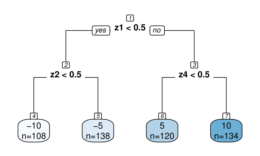
Figure S1: Fit of the tree

We then estimate omics effects $\hat{\boldsymbol{\beta}}$as a function of penalty $\alpha$ for the $\lambda$ grid. We show estimates for $\beta_{2}=0.62,$ which interacts with $\boldsymbol{z}_{i},$ and $\beta_{6}=-0.92,$ which does not interact with $z_{i}.$ In addition, we show the estimated constant $c_{6}$ in node $6$ (Figure S1), whose true value equals $c_{6}=5.$

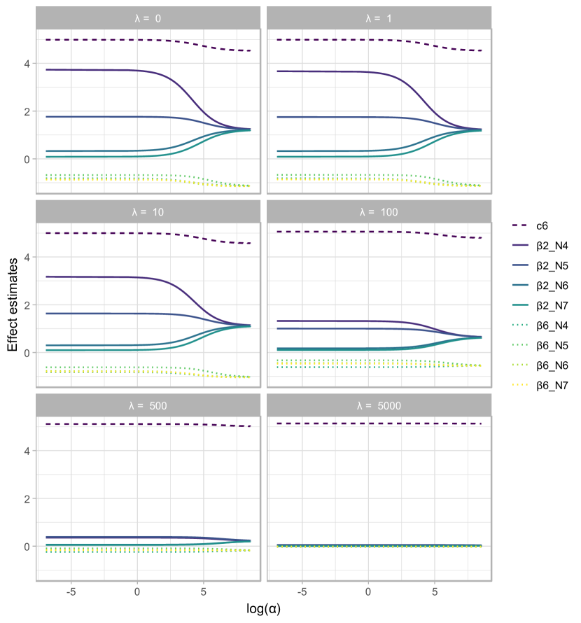
Figure S2: Regularization plots as a function of fusion penalty $\alpha$ for several values of $\lambda$. For illustration purposes, we only depict the node-specific estimates of $\beta_{2},$ $\beta_{6}$ and the clinical intercept estimated in node $6,$ i.e. $c_{6}.$

Results are depicted in Figure (S2). For small $\alpha$, and $\lambda<500,$ the node-specific estimates of $\beta_{2}$ vary substantially, which is expected because there is a strong interaction effect between this omics covariate and the clinical covariates. Estimates of $\beta_{6}$ remain relatively stable across nodes, which is also expected as for this omics covariate no interactions are present. For large $\alpha,$ the node-specific effects of $\beta_{2}$ are shrunken towards a shared value. Figure (S2) also shows that larger $\lambda$ values shrink the node-specific omics effect estimates towards $0,$ as expected. The clinical intercept $c_{6},$ which is left unpenalized slightly decreases for large $\alpha.$ Because $c$ and $\beta$ are estimated jointly, penalization of $\beta$ by the fusion penalty introduces bias in estimation of $c$ (see limit (15)) This bias becomes smaller for larger $\lambda$ and diminishes for $\lim_{\lambda\rightarrow\infty},$ i.e. limit (12).

6 Global Test summary

We shortly summarize the global test methodology (Goeman et al., 2006) applied to FusedTree. In node $m,$ we have data $\mathcal{D}_{m}=\left\{y_{k}^{(m)},\boldsymbol{x}_{k}^{(m)}\right\}_{k=1}^{n_{m}}$ and we model the response by:

$$E\left(y_{k}^{(m)}\mid\boldsymbol{x}_{i}^{(m)}\right)=c_{m}+\sum_{j=1}^{p}x_{kj}^{(m)}\beta_{j}^{(m)}.$$

We then test:

$$H_{0}:\quad\beta_{1}^{(m)}=\beta_{2}^{(m)}=\dots=\beta_{p}^{(m)}=0,$$

which is infeasible using a standard F-test for $p>n_{m}.$ To make progress, it is assumed that elements of $\boldsymbol{\beta}_{(m)}$ come from a common distribution with zero mean and variance $\tau^{2}.$ The method then tests

$$H_{0}:\quad\tau^{2}=0,$$

using the score test statistic. Because this statistic is asymptotically normal under $H_{0}$, p-values may be computed from this asymptotic distribution. Alternatively, for small sample sizes, the empirical distribution for the test statistic may be determined using permutations. The global test method also applies to binary $y_{i}\in\left\{0,1\right\}$ and survival response. For full details, see (Goeman et al., 2004).

7 Simulations results

Here, we show the full descriptions and results of the simulations summarized in Section $4$ of the main text.

We conduct three simulation experiments with different functional relationships $f_{1},$ $f_{2},$ $f_{3}$ between the response $y$ and clinical $\boldsymbol{z}$ and omics covariates $\boldsymbol{x}$ to showcase FusedTree:

1. Interaction (Section 7.1). We specify $f_{1}$ inspired by model (1) of the main text. Thus $f_{1}$ is a tree, defined by clinical covariates, with different linear omics models in the leaf nodes for $25\%$ of the omics covariates. The remaining $75\%$ of the omics covariates has a constant effect size. Thus, the clinical covariates interact with $25\%$ of the omics covariates.

2. Full Fusion (Section 7.2). In this experiment, we specify $f_{2}$ by two separate parts, a nonlinear clinical part and a linear omics part. In this experiment, the clinical covariates do not act as effect modifiers and FusedTree would benefit from a large fusion penalty $\alpha.$

3. Linear (Section 7.3). In this experiment, we specify $f_{3}$ by a separate linear clinical and a linear omics part. Again, FusedTree would benefit from a large fusion penalty $\alpha.$

The set-up for the three experiments is as follows. We simulate response $y_{i}=f\left(\boldsymbol{z}_{i},\boldsymbol{x}_{i}\right)+\epsilon_{i},$ with $\epsilon_{i}\sim\mathcal{N}\left(0,1\right)$ for $i=1,\ldots,N,$ and with different $f\left(\cdot\right)$ for each experiment. We consider two simulation settings: $N=100$ and $N=300.$ For each experiment and for each setting, we simulate clinical covariates $\boldsymbol{z}_{il}\sim\textrm{Unif}\left(0,1\right),$ for $l=1,\ldots,q$ and $q=5,$ and omics covariates $\boldsymbol{x}_{i}\sim\mathcal{N}\left(\boldsymbol{0}_{p},\boldsymbol{\Sigma}_{p\times p}\right),$ with $p=500,$ and correlation matrix $\boldsymbol{\Sigma}_{p\times p}$ set to the estimate of a real omics data set (Best et al., 2015) of which we randomly select $p=500$ covariates. For correlation matrix estimation, we employ work by Schäfer and Strimmer [2005] implemented in the R package corpcor. Finally, we simulate elements $j=1,\ldots,p$ of the omics effect regression parameter vector by $\beta_{1},\ldots,\beta_{p}\sim\textrm{Laplace}(0,\theta),$ with scale parameter $\theta.$ The Laplace distribution is the prior density for Bayesian lasso regression and ensures many close-to-zero effect sizes. We tune $\theta$ to control the signal in the omics covariates. Specifics of this parameter are found in the subsections.

In each experiment and for each setting, we simulate $500$ data sets. To each data set, we fit FusedTree and several competitors: ridge regression and lasso regression with unpenalized $\boldsymbol{z}_{i}$ implemented in the R package porridge (van Wieringen and Aflakparast, 2024) and glmnetFriedman et al. [2010], respectively, random forest (RF) implemented in the R package randomforestSRC (Ishwaran et al., 2008), and gradient boosting (Friedman, 2001) (GB) implemented in the R package gbm (Ridgeway, 2004). To assess the benefit of tuning fusion penalty $\alpha,$ we also fit FusedTree with $\alpha=0$ (ZeroFus), and Fully FusedTree (FulFus). Fully FusedTree jointly estimates a separate clinical part, defined by the estimated tree, and a separate omics part that does not vary with respect to the clinical covariates. For experiment $1$, we also include an oracle tree model. This model knows the tree structure in advance and only estimates the regression parameters in the leaf nodes and tunes $\lambda$ and $\alpha$. For all FusedTree-based models, we also include all continuous clinical covariates $\boldsymbol{z}_{i}$ linearly in the regression model, as explained in Section 2.6 of the main text.

We compare prediction models using the prediction mean square error (PMSE): $N^{-1}\sum_{i=1}^{N}\left(y_{i}-\hat{y}_{i}\right)^{2},$ with $\hat{y}_{i}$ the prediction of the given model for observation $i.$ The PMSE is estimated on an independent test data set of size $N_{\textrm{test}}=5,000.$ We summarize the PMSEs over the $500$ simulated data sets using boxplots. Finally, we tune the hyperparameter of all considered prediction models by $5$-fold cross validation. For FusedTree, we first prune the tree and then tune $\lambda$ and $\alpha,$ for ridge and lasso regression, we tune the standard penalties, and for gradient boosting, we tune the learning rate and the number of trees. We do not tune random forest because it is relatively robust to different hyperparameter settings.

7.1 Interaction between clinical and omics covariates

We specify the relationship $f_{1}$ between response and clinical and omics covariates by

$$f_{1}\left(\boldsymbol{x},\boldsymbol{z},\boldsymbol{\beta}\right) =I\left(z_{1}\leq\frac{1}{2}\right)I\left(z_{2}\leq\frac{1}{2}\right)\left(-10+8\boldsymbol{x}_{1:125}^{\top}\boldsymbol{\beta}_{1:125}\right)$$

$$+I\left(z_{1}\leq\frac{1}{2}\right)I\left(z_{2}>\frac{1}{2}\right)\left(-5+2\boldsymbol{x}_{1:125}^{\top}\boldsymbol{\beta}_{1:125}\right)$$

$$+I\left(z_{1}>\frac{1}{2}\right)I\left(z_{4}\leq\frac{1}{2}\right)\left(5+\frac{1}{2}\boldsymbol{x}_{1:125}^{\top}\boldsymbol{\beta}_{1:125}\right)$$

$$+I\left(z_{1}>\frac{1}{2}\right)I\left(z_{4}>\frac{1}{2}\right)\left(10+\frac{1}{8}\boldsymbol{x}_{1:125}^{\top}\boldsymbol{\beta}_{1:125}\right)$$

$$+\boldsymbol{x}_{126:500}^{\top}\boldsymbol{\beta}_{126:500.}+3z_{3}.$$

The scale parameter of the Laplace distribution equals $\theta=10/p.$ Clinical covariates $\boldsymbol{z}$ contain one noise covariate: $z_{5},$ and $4$ predictive covariates: tree covariates $z_{1},$ $z_{2},$ and $z_{4}$ and linear covariate $z_{3}.$ The predictive clinical covariates interact with the first $25\%$ of omics covariates, while the last $75\%$ of omics covariates have a constant effect size.

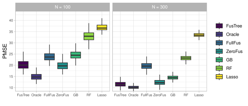
Figure S3: Boxplots of prediction mean square errors for several learners across $500$ simulated data sets for $N=100$ and $N=300$ for the interaction simulation experiment. For illustration purposes, we excluded ridge regression because it performed much worse compared to the other models.

FusedTree clearly outperforms FulFus and competitors GB, RF, and lasso for both sample size settings (Figure S3 and Table S1). We excluded results for ridge regression because it performed much worse than the other models.

The oracle model performs better than FusedTree indicating that the tree structure is not always estimated reliably. This difference becomes smaller for a larger sample size because tree structure estimation improves. For $N=100,$ FusedTree with $\alpha=0$ (ZeroFus) has a slightly lower average PMSE than FusedTree, while FusedTree has a lower PMSE than ZeroFus for $N=300.$ Supplementary Figure S4 reveals that for $N=100,$ fusion penalty parameter $\alpha$ is in some cases rather large, which explains why ZeroFus performs slightly better. For $N=300,$ $\alpha$ is tuned more reliably by FusedTree. Consequently, FusedTree has a lower average PMSE than ZeroFus.

Table S1: Average PMSE for several learners for the interaction simulation experiment

	$\boldsymbol{N=100}$	$\boldsymbol{N=300}$
FusedTree	$20.5$	$11.6$
Oracle	$14.9$	$10.2$
FulFus	$24.1$	$19.8$
ZeroFus	$20.0$	$12.5$
GB	$24.7$	$14.5$
RF	$33.0$	$23.2$
Ridge	$50.6$	$47.2$
Lasso	$37.5$	$33.5$

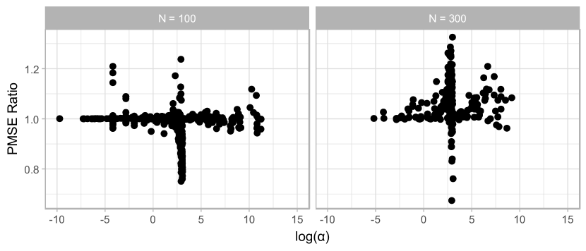
Figure S4: Scatter plot of $\textrm{PMSE}_{\textrm{ZeroFus}}/\textrm{PMSE}_{\textrm{FusedTree}}$ as a function of fusion penalty $\alpha$ (log scale) across $500$ simulated data sets for $N=100$ and $N=300$ for the effect modification simulation experiment (Section 4.1)

7.2 Full Fusion

For the full fusion experiment, we specify $f_{2}$ by

$$f_{2}\left(\boldsymbol{x},\boldsymbol{z},\boldsymbol{\beta}\right)=15\sin\left(\pi z_{1}z_{2}\right)+10\left(z_{3}-\frac{1}{2}\right)^{2}+2\exp\left(z_{4}\right)+2z_{5}+\boldsymbol{x}^{\top}\boldsymbol{\beta}.$$ (18)

We set the scale parameter of the Laplace distribution to $\theta=75/p,$ which ensures that the clinical covariate part explains slightly more variance in the response compared to the omics covariate part.

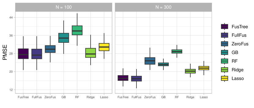
Figure S5: Boxplots of prediction mean square errors for several learners across $500$ simulated data sets for $N=100$ and $N=300$ for the full fusion simulation experiment

Figure S5 and Table S2 reveal that FusedTree and FulFus perform similarly for both sample sizes. Figure S6 plots the PMSE ratio of FulFus and FusedTree across simulated data sets as a function of the tuned fusion penalty $\alpha.$ This plot shows that $\alpha$ is typically set to a large value in which case the ratio is close to $1.$ For the few cases that the tuned $\alpha$ is small, FulFus outperforms FusedTree. FusedTree has a lower PMSE compared to ZeroFus, especially for $N=300.$ This finding suggests a clear benefit of borrowing information across nodes compared to independently estimating the omics effects.

FusedTree has a lower PMSE compared to competitors ridge and lasso regression, random forest, and gradient boosting, although the difference with ridge and lasso regression is small for $N=100.$

Table S2: Average PMSE for several learners for the full fusion simulation experiment

	$\boldsymbol{N=100}$	$\boldsymbol{N=300}$
FusedTree	$27.9$	$17.4$
FulFus	$27.8$	$17.2$
ZeroFus	$30.0$	$24.8$
GB	$35.0$	$23.3$
RF	$38.2$	$29.0$
Ridge	$28.2$	$20.5$
Lasso	$31.1$	$21.6$

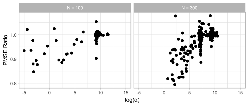
Figure S6: Scatter plot of $\textrm{PMSE}_{\textrm{Full\,Fus}}/\textrm{PMSE}_{\textrm{FusedTree}}$ as a function of fusion penalty $\alpha$ (log scale) across $500$ simulated data sets for $N=100$ and $N=300$ for the full fusion simulation experiment (Section 4.2)

7.3 Linear

For the linear experiment, we specify $f_{3}$ by

$$f_{3}\left(\boldsymbol{x},\boldsymbol{z},\boldsymbol{c},\boldsymbol{\beta}\right)=\boldsymbol{z}^{\top}\boldsymbol{c}+\boldsymbol{x}^{\top}\boldsymbol{\beta},$$

with elements $c_{l}\sim\textrm{Laplace}\left(\frac{75}{p}\right)$ of clinical regression parameter $\boldsymbol{c}\in\mathbb{R}^{5},$ and elements $\beta_{j}\sim\textrm{Laplace}\left(\frac{35}{p}\right)$ of omics regression parameter vector $\boldsymbol{\beta}\in\mathbb{R}^{500}.$ The linear clinical part explains slightly more variation in $y$ compared to the linear omics part.

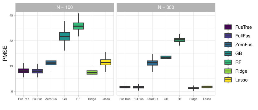
Figure S7: Boxplots of prediction mean square errors for several learners across $500$ simulated data sets for $N=100$ and $N=300$ for the linear simulation experiment

FusedTree clearly outperforms the nonlinear competitors GB and RF (Figure S7 and Table S3). For both sample size settings, FusedTree has a slightly larger PMSE compared to ridge regression. This difference becomes smaller for $N=300$ compared to $N=100.$ FusedTree performs slightly better than lasso regression for $N=100$, while for $N=300$ performance is similar.

Compared to FulFus, FusedTree performs nearly identical. Therefore, the benefit of fully fusing the omics effects in advance compared to estimating the fusion strength is negligible for this simulation experiment. Again, FusedTree has a lower PMSE than ZeroFus because of the benefit of borrowing information across nodes.

Table S3: Average PMSE for several learners for the linear simulation experiment

	$\boldsymbol{N=100}$	$\boldsymbol{N=300}$
FusedTree	$16.7$	$8.23$
FulFus	$16.5$	$8.17$
ZeroFus	$20.8$	$20.3$
GB	$34.6$	$23.6$
RF	$39.6$	$32.5$
Ridge	$15.8$	$7.62$
Lasso	$21.0$	$8.29$

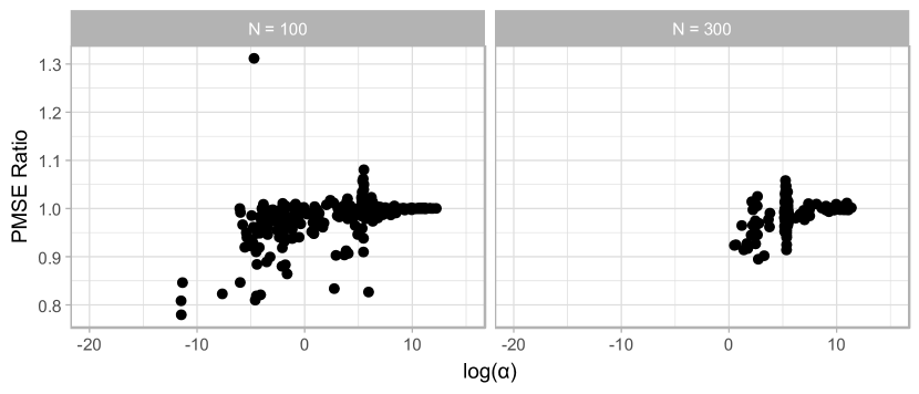
Figure S8: Scatter plot of $\textrm{PMSE}_{\textrm{Full\,Fus}}/\textrm{PMSE}_{\textrm{FusedTree}}$ as a function of fusion penalty $\alpha$ (log scale) across $500$ simulated data sets for $N=100$ and $N=300$ for the linear simulation experiment (Section 4.3)

8 Survival curves for CRC application

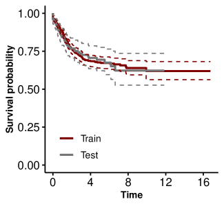
Figure S9: Kaplan-Meier estimate of the overall survival probability of the training and test response as a function of time (in years). The plot is produced using the R package survminer

References

• Best etย al. [2015] M.ย G. Best, N.ย Sol, I.ย Kooi, J.ย Tannous, B.ย A. Westerman, F.ย Rustenburg, P.ย Schellen, H.ย Verschueren, E.ย Post, J.ย Koster, etย al. Rna-seq of tumor-educated platelets enables blood-based pan-cancer, multiclass, and molecular pathway cancer diagnostics. Cancer cell, 28(5):666โ€“676, 2015. doi: 10.1016/j.ccell.2015.09.018.
• Friedman etย al. [2010] J.ย Friedman, R.ย Tibshirani, and T.ย Hastie. Regularization paths for generalized linear models via coordinate descent. J Stat Softw, 33(1):1โ€“22, 2010. doi: 10.18637/jss.v033.i01.
• Friedman [2001] J.ย H. Friedman. Greedy function approximation: A gradient boosting machine. Ann Stat, 29(5):1189 โ€“ 1232, 2001. doi: 10.1214/aos/1013203451. URL https://doi.org/10.1214/aos/1013203451.
• Goeman etย al. [2004] J.ย J. Goeman, S.ย A. vanย de Geer, F.ย deย Kort, and H.ย C. van Houwelingen. A global test for groups of genes: testing association with a clinical outcome. Bioinformatics, 20(1):93โ€“99, 2004. ISSN 1367-4803. doi: 10.1093/bioinformatics/btg382. URL https://doi.org/10.1093/bioinformatics/btg382.
• Goeman etย al. [2006] J.ย J. Goeman, S.ย A. Van Deย Geer, and H.ย C. Vanย Houwelingen. Testing against a high dimensional alternative. J R Stat Soc Ser B Methodol, 68(3):477โ€“493, 2006. doi: https://doi.org/10.1111/j.1467-9868.2006.00551.x. URL https://rss.onlinelibrary.wiley.com/doi/abs/10.1111/j.1467-9868.2006.00551.x.
• Ishwaran etย al. [2008] H.ย Ishwaran, Udayaย B. K., B.ย H. Eugene, and L.ย S. Michael. Random survival forests. Ann Appl Stat, 2(3), 2008. ISSN 1932-6157. doi: 10.1214/08-aoas169.
• Khatri and Rao [1968] C.ย G. Khatri and C.ย R. Rao. Solutions to some functional equations and their applications to characterization of probability distributions. The Indian Journal of Statistics, Series A (1961-2002), 30(2):167โ€“180, 1968. URL http://www.jstor.org/stable/25049527.
• Lettink etย al. [2023] A.ย Lettink, M.ย Chinapaw, and W.ย N. van Wieringen. Two-dimensional fused targeted ridge regression for health indicator prediction from accelerometer data. R Stat Soc Ser C Appl, 72(4):1064โ€“1078, 2023. ISSN 0035-9254. doi: 10.1093/jrsssc/qlad041. URL https://doi.org/10.1093/jrsssc/qlad041.
• Nelder and Mead [1965] J.ย A. Nelder and R.ย Mead. A Simplex Method for Function Minimization. Comput J, 7(4):308โ€“313, 1965. doi: 10.1093/comjnl/7.4.308. URL https://doi.org/10.1093/comjnl/7.4.308.
• Ridgeway [2004] G.ย Ridgeway. The gbm package. R Foundation for Statistical Computing, 5(3), 2004.
• Schรคfer and Strimmer [2005] J.ย Schรคfer and K.ย Strimmer. A shrinkage approach to large-scale covariance matrix estimation and implications for functional genomics. Stat Appl Genet Mol Biol, 4(1):Article32, 2005. doi: 10.2202/1544-6115.1175.
• Slyusar [1999] V.ย I. Slyusar. A family of face products of matrices and its properties. Cybern Syst Anal, 35(3):379โ€“384, 1999. doi: 10.1007/BF02733426. URL https://doi.org/10.1007/BF02733426.
• vanย de Wiel etย al. [2021] M.ย A. vanย de Wiel, M.ย M. van Nee, and A.ย Rauschenberger. Fast cross-validation for multi-penalty high-dimensional ridge regression. J Comput Graph Stat, 30(4):835โ€“847, 2021. doi: 10.1080/10618600.2021.1904962. URL https://doi.org/10.1080/10618600.2021.1904962.
• van Houwelingen etย al. [2006] H.ย C. van Houwelingen, T.ย Bruinsma, A.ย A.ย M. Hart, L.ย J. vanโ€™t Veer, and L.ย F.ย A. Wessels. Cross-validated cox regression on microarray gene expression data. Stat Med, 25(18):3201โ€“3216, 2006. doi: https://doi.org/10.1002/sim.2353. URL https://onlinelibrary.wiley.com/doi/abs/10.1002/sim.2353.
• van Wieringen and Aflakparast [2024] W.ย N. van Wieringen and M.ย Aflakparast. porridge: Ridge-Type Estimation of a Potpourri of Models, 2024. URL https://CRAN.R-project.org/package=porridge. R package version 0.3.3.