Abstract

In causal inference, treatment effects are typically estimated under the ignorability, or unconfoundedness, assumption, which is often unrealistic in observational data. By relaxing this assumption and conducting a sensitivity analysis, we introduce novel bounds and derive confidence intervals for the Average Potential Outcome (APO) – a standard metric for evaluating continuous-valued treatment or exposure effects. We demonstrate that these bounds are sharp under a continuous sensitivity model, in the sense that they give the smallest possible interval under this model, and propose a doubly robust version of our estimators. In a comparative analysis with the method of [17], using both simulated and real datasets, we show that our approach not only yields sharper bounds but also achieves good coverage of the true APO, with significantly reduced computation times.

1 INTRODUCTION

Estimating the causal effects of continuous interventions is crucial across many domains, including life sciences or economics. Understanding the impact of air pollutant concentration on cardiovascular mortality, drug concentration in plasma on tumor size, or income on demand for goods or services are examples of such applications of interest. In particular, observational data, or more generally real-world data, offer a significant opportunity to enhance clinical drug development and support regulatory decisions by using, for instance, Electronic Health Records (EHR), medical claims data or measurements from wearable devices. Since the 21^st Century Cures Act, the United States Food and Drug Administration (FDA) has even been requested to develop a program in order to evaluate how real-world evidence could be used for medical product approvals [6].

To leverage observational data in the context of treatment effect estimation, several statistical methodologies have been developed for binary and continuous treatments. Most of these approaches rely on a strong assumption, known as ignorability, unconfoundedness or exogeneity [31] in causal inference. This assumption posits that, inside a subgroup of units that share similar observed characteristics, the treatment can be considered randomly assigned. In the case of continuous treatments, the Average Potential Outcome (APO), sometimes named dose-response function, stands out as a metric of reference to evaluate treatment effect. Among the various methods that assume ignorability, noteworthy estimation approaches of the APO include Inverse Probability Weighting-like methods [15, 14, 22, 20, 5], Bayesian Additive Regression Trees (BART) [13], and Adversarial CounterFactual Regression (ACFR) [21]. The conditional counterpart of the APO, the Conditional Average Potential Outcome (CAPO), can also be estimated via similar techniques.

Nevertheless, this hypothesis may be overly optimistic given the impossibility to observe all confounding variables, especially in observational studies. To overcome this issue, recent works have suggested using sensitivity models to bound the biased treatment effect estimates, providing intervals as solutions. In the binary treatment scenario, researchers have explored ways to deviate from the regular ignorability assumption through the Marginal Sensitivity Model (MSM) [34, 39, 7, 8] or Rosenbaum’s Sensitivity Model (RSM) [28, 38].

Following these works, [17] extended the MSM to the continuous case (Continuous Marginal Sensitivity Model, or CMSM) and provided bounds for the APO that are suitable for high-dimensional and large-sample data. In this paper, we propose a new methodology that combines the doubly robust kernel-based APO estimator from [20] with an additional constraint on a weight function, and derive sharp bounds under a sensitivity model introduced in Section 2. Then, we deduce confidence intervals (CI) via the percentile bootstrap method, as done in [39]. This novel approach provides tighter and faster-to-compute bounds for the APO, as compared to [17].

1.1 Outline

The paper is organized as follows. Problem setting and notations are presented in Section 2. Section 3 provides a detailed description of the novel APO and CAPO bounds, along with convergence results. Empirical results and comparisons with the method from [17] are presented in Section 4 on simulated and real datasets, supporting our theoretical findings while displaying the computational efficiency of our estimators. Additional theoretical details, proofs and experimental results are provided in the appendices.

2 PROBLEM SETTING AND NOTATIONS

2.1 Notations and Assumptions

In the following, we consider the Neyman-Rubin potential outcome framework [25, 31] adapted to continuous treatments. We denote by $\mathbf{X}\in\mathcal{X}\subset\mathbb{R}^{p_{\mathbf{X}}}$ the vector of observed confounders, with $p_{\mathbf{X}}\geq 1$, $T\in\mathcal{T}\subset\mathbb{R}$ the continuous treatment or exposition, and $Y(t)\in\mathcal{Y}\subset\mathbb{R}$ the potential outcome for a treatment value $t$. If $Y$ is the observed outcome and $T=t$, then we assume that $Y=Y(t)$ (consistency and non-interference). Estimated quantities are denoted with a hat $\hat{\cdot}$, unless stated otherwise. Conditional expectations are rather written with a subscript, e.g. $\mathbb{E}_{\mathbf{X}=\mathbf{x}}[Y]\overset{\mathrm{not.}}{=}\operatorname*{\mathbb{E}}[Y|\mathbf{X}=\mathbf{x}]$.

For a fixed treatment or exposition value $\tau\in\mathcal{T}$ and covariate vector $\mathbf{x}\in\mathcal{X}$, we are interested in estimating and bounding the APO $\theta(\tau)$ and CAPO $\theta(\tau,\mathbf{x})$, which are defined as

$$\theta(\tau)\coloneq\operatorname*{\mathbb{E}}[Y(\tau)]\quad\text{and}\quad\theta(\tau,\mathbf{x})\coloneq\mathbb{E}_{\mathbf{X}=\mathbf{x}}[Y(\tau)].$$

The APO and CAPO are commonly estimated under the ignorability assumption for continuous treatments [14, 22, 20]:

$$\forall t\in\mathcal{T},\,Y(t)\mathchoice{\mathrel{\hbox to0.0pt{$\displaystyle\perp$\hss}\mkern 2.0mu{\displaystyle\perp}}}{\mathrel{\hbox to0.0pt{$\textstyle\perp$\hss}\mkern 2.0mu{\textstyle\perp}}}{\mathrel{\hbox to0.0pt{$\scriptstyle\perp$\hss}\mkern 2.0mu{\scriptstyle\perp}}}{\mathrel{\hbox to0.0pt{$\scriptscriptstyle\perp$\hss}\mkern 2.0mu{\scriptscriptstyle\perp}}}T\mid\mathbf{X}.$$

For convenience, we will refer to it as $\mathbf{X}$-ignorability. Under this hypothesis and consistency of the outcomes, notice that

$$\theta(\tau) =\operatorname*{\mathbb{E}}[\theta(\tau,\mathbf{X})]=\operatorname*{\mathbb{E}}[\mathbb{E}[Y(\tau)|\mathbf{X}]]$$

$$=\operatorname*{\mathbb{E}}[\mathbb{E}_{\mathbf{X},T=\tau}[Y(T)]]=\operatorname*{\mathbb{E}}[\eta(\tau,\mathbf{X})]$$ (1)

where $\eta(t,\mathbf{x})\coloneq\mathbb{E}_{\mathbf{X}=\mathbf{x},T=t}[Y]$ is a conditional expectation that could be estimated by regression. [20] and [5] proposed simple, stabilized and/or doubly robust versions of a kernel-based estimator of the APO, all recalled in Appendix A.3. We focus here on the doubly robust estimator from [20]. For a fixed treatment value $\tau\in\mathcal{T}$, and considering an i.i.d. observed sample $\mathcal{D}=\{(\mathbf{X}_{i},T_{i},Y_{i})\}_{i=1}^{n}$ of size $n$, they express it as

$$\hat{\theta}_{h}(\tau) =\frac{1}{n}\sum_{i=1}^{n}\frac{K_{h}(T_{i}-\tau)}{\hat{f}(T=T_{i}|\mathbf{X}=\mathbf{X}_{i})}\bigl{(}Y_{i}-\hat{\eta}(T_{i},\mathbf{X}_{i})\bigr{)}$$

$$\quad+\hat{\eta}(\tau),$$ (2)

where $\hat{\eta}(\tau)=\sum_{i=1}^{n}\hat{\eta}(\tau,\mathbf{X}_{i})/n$. $K_{h}$ is defined as $K_{h}(s)=K(s/h)/h$, where $h>0$ is a bandwidth and $K$ is a kernel. Common choices of $K$ include the Epanechnikov or Gaussian kernels. $K_{h}$ is here to localize the estimation around the treatment of interest $\tau$. See Assumption A.5 in appendix for more details on the kernel.

The density of $T$ conditionally on $\mathbf{X}=\mathbf{x}$, $t\mapsto f(T=t|\mathbf{X}=\mathbf{x})$, is known as Generalized Propensity Score (GPS) [14]. Reweighting the observed outcomes $Y_{i}$s by the inverse of the GPS gives more importance to units that had less chance to be exposed to treatment $T_{i}$ and, thus, artificially rebalances the data. The GPS generalizes the common Propensity Score [29] used in the binary treatment case. We assume that the GPS exists and that it is positive for all $\mathbf{x}\in\mathcal{X}$ and $t\in\mathcal{T}$ (see Assumption A.3 of positivity in appendix).

However, as mentioned earlier, $\mathbf{X}$-ignorability is rarely satisfied in practice due to the presence of unobserved confounders $\mathbf{U}\in\mathcal{U}\subset\mathbb{R}^{p_{\mathbf{U}}}$, where $p_{\mathbf{U}}\geq 1$. A more reasonable assumption is to impose $(\mathbf{X},\mathbf{U})$-ignorability:

$$\forall t\in\mathcal{T},\,Y(t)\mathchoice{\mathrel{\hbox to0.0pt{$\displaystyle\perp$\hss}\mkern 2.0mu{\displaystyle\perp}}}{\mathrel{\hbox to0.0pt{$\textstyle\perp$\hss}\mkern 2.0mu{\textstyle\perp}}}{\mathrel{\hbox to0.0pt{$\scriptstyle\perp$\hss}\mkern 2.0mu{\scriptstyle\perp}}}{\mathrel{\hbox to0.0pt{$\scriptscriptstyle\perp$\hss}\mkern 2.0mu{\scriptscriptstyle\perp}}}T|\mathbf{X},\mathbf{U}.$$

Under this assumption, the final equality in (2.1) no longer holds, meaning that $\theta(\tau)\neq\operatorname*{\mathbb{E}}[\eta(\tau,\mathbf{X})]$, and the estimator of the APO from Equation (2.1) becomes biased. In what follows, we show that, under $(\mathbf{X},\mathbf{U})$-ignorability and a sensitivity model introduced in the next subsection, bounds for the APO and CAPO can be derived and subsequently estimated. This is consistent with findings from [17], except that we propose sharp bounds.

2.2 Continuous Marginal Sensitivity Model

As mentioned in Section 1, previous works suggested bounding binary causal treatment effects under the MSM from [34] in presence of unobserved confounders. This sensitivity model involves an odds ratio of propensity scores that is bounded by a user-defined sensitivity parameter. Under absolute continuity assumptions, [17] later extended this model to the continuous treatment case via a likelihood ratio. We recall their model in Appendix A.1. In this paper, we introduce a new Continuous Marginal Sensitivity Model (CMSM) and show that it induces the one from [17].

Definition 2.1.

(CMSM for the APO) Under positivity Assumption A.3, for a given treatment value $\tau\in\mathcal{T}$, for all $(\mathbf{x},\mathbf{u})\in\mathcal{X}\times\mathcal{U}$, there exists a sensitivity parameter $\Gamma\geq 1$ such that

$$\Gamma^{-1}\leq\frac{f(T=\tau|\mathbf{X}=\mathbf{x},\mathbf{U}=\mathbf{u})}{f(T=\tau|\mathbf{X}=\mathbf{x})}\leq\Gamma.$$ (3)

The CMSM involves a conditional density with respect to $\mathbf{X}=\mathbf{x}$ and $\mathbf{U}=\mathbf{u}$, $t\mapsto f(T=t|\mathbf{X}=\mathbf{x},\mathbf{U}=\mathbf{u})$, which is the true but inestimable Generalized Propensity Score, had we observed all possible confounders. As compared to the sensitivity model from [17], our model does not involve the potential outcome $Y(\tau)$. For the CAPO, the same definition applies but for a fixed treatment value $\tau$ and fixed vector of covariates $\mathbf{x}$.

We can show that the proposed CMSM implies the one considered in [17]. This idea is formalized in the following proposition.

Proposition 2.2.

For a given treatment value $\tau\in\mathcal{T}$, for all $(\mathbf{x},y)\in\mathcal{X}\times\mathcal{Y}$, under the CMSM from Definition 2.1 and Assumptions A.3 and A.4, the following ratio

$$\frac{f(T=\tau|\mathbf{X}=\mathbf{x},Y(\tau)=y)}{f(T=\tau|\mathbf{X}=\mathbf{x})}=\frac{f(Y=y|\mathbf{X}=\mathbf{x},T=\tau)}{f(Y(\tau)=y|\mathbf{X}=\mathbf{x})}$$

$$=\frac{f(Y(\tau)=y|\mathbf{X}=\mathbf{x},T=\tau)}{f(Y(\tau)=y|\mathbf{X}=\mathbf{x})}$$

lies in $[\Gamma^{-1},\Gamma]$.

See Appendix A.7 for a proof. Now, $\Gamma$ can be seen as a user-defined sensitivity parameter which measures the deviation from the usual $\mathbf{X}$-ignorability assumption: if $\Gamma=1$, the CMSM becomes equivalent to $\mathbf{X}$-ignorability, as if all confounders were observed; higher values of $\Gamma$ assume a greater effect of the unobserved confounders on the treatment $T$ and a deviation from $\mathbf{X}$-ignorability. Under the model from Definition 2.1, we can now derive bounds for the CAPO and APO in the next section.

3 BOUNDS FOR THE CAPO AND APO

In this section, we present novel bounds for the CAPO and APO in the presence of unobserved confounders. They rely on a constraint on a likelihood ratio that we leverage to reach sharp bounds under the CMSM in Theorem 3.1. Additionally, we show that our bounds are also sharper than the ones considered in [17].

3.1 Weight Function

To reach the desired solution, we start by working on the CAPO until Theorem 3.1, and extend the results to the APO afterwards. Notice first that, by positivity Assumption A.4, the CAPO can be rewritten

$$\theta(\tau,\mathbf{x}) \coloneq\mathbb{E}_{\mathbf{X}=\mathbf{x}}[Y(\tau)]=\int yf(Y(\tau)=y|\mathbf{X}=\mathbf{x})\,\mathrm{d}y$$

$$=\int y\,w^{\star}(y,\mathbf{x},\tau)f(Y=y|\mathbf{X}=\mathbf{x},T=\tau)\,\mathrm{d}y$$

$$=\mathbb{E}_{\mathbf{X}=\mathbf{x},T=\tau}[Yw^{\star}(Y,\mathbf{x},\tau)],$$

where, for all $(\mathbf{x},t,y)\in\mathcal{X}\times\mathcal{T}\times\mathcal{Y}$,

$$w^{\star}(y,\mathbf{x},t)\coloneq\frac{f(Y(t)=y|\mathbf{X}=\mathbf{x})}{f(Y=y|\mathbf{X}=\mathbf{x},T=t)}$$

exists [17]. Note that the weight function, or likelihood ratio, $w^{\star}$ fulfills the constraint

$$\mathbb{E}_{\mathbf{X}=\mathbf{x},T=t}[w^{\star}(Y,\mathbf{x},t)]=1$$ (4)

for all $(\mathbf{x},t)\in\mathcal{X}\times\mathcal{T}$, and takes values within $[\Gamma^{-1},\Gamma]$, according to Proposition 2.2. For computation details, refer to Appendix A.4.

Using the conditional expectation $\eta$ and the previous constraint (4), the CAPO can also be written

$$\theta(\tau,\mathbf{x}) =\mathbb{E}_{\mathbf{X}=\mathbf{x},T=\tau}\bigl{[}\bigl{(}Y-\eta(\tau,\mathbf{x})\bigr{)}w^{\star}(Y,\mathbf{x},\tau)\bigr{]}$$

$$\quad+\eta(\tau,\mathbf{x}).$$ (5)

3.2 Sharp Bounds for the CAPO and APO

Under the CMSM, we define the bounds for the CAPO as

$$\theta^{-}(\tau,\mathbf{x}) \coloneq\inf_{w\in\mathcal{W}^{\star}_{\tau}}\mathbb{E}_{\mathbf{X}=\mathbf{x},T=\tau}\bigl{[}\bigl{(}Y-\eta(\tau,\mathbf{x})\bigr{)}w(Y,\mathbf{x},\tau)\bigr{]}$$

$$\quad+\eta(\tau,\mathbf{x}),$$ (6)

$$\theta^{+}(\tau,\mathbf{x}) \coloneq\sup_{w\in\mathcal{W}^{\star}_{\tau}}\mathbb{E}_{\mathbf{X}=\mathbf{x},T=\tau}\bigl{[}\bigl{(}Y-\eta(\tau,\mathbf{x})\bigr{)}w(Y,\mathbf{x},\tau)\bigr{]}$$

$$\quad+\eta(\tau,\mathbf{x}),$$ (7)

where $\mathcal{W}^{\star}_{\tau}$ is the set of functions $w:\mathcal{Y}\times\mathcal{X}\times\mathcal{T}\to[\Gamma^{-1},\Gamma]$ that satisfy Equation (4). In other words, these bounds correspond to the lowest and highest possible values for the CAPO when the weight function varies in $\mathcal{W}^{\star}_{\tau}$. Results from convex analysis allow to solve the minimization and maximization problems and lead to the results given in the following theorem.

Theorem 3.1.

Under Assumption A.3 and our sensitivity model from Definition 2.1, the solutions to the optimization problems (6) and (7) are given by

$$\theta^{\pm}(\tau,\mathbf{x}) =\frac{2\gamma-1}{\gamma}\mathbb{E}_{\mathbf{X}=\mathbf{x},T=\tau}\Bigl{[}Y-\eta(\tau,\mathbf{x})\Big{|}Q^{\pm}_{\mathbf{X},\tau}\Bigr{]}$$

$$\quad+\eta(\tau,\mathbf{x})$$ (8)

where $\pm$ stands for either $+$ or $-$, $Q^{+}_{\mathbf{X},\tau}\coloneq\{Y>q_{\gamma}^{\mathbf{X},\tau}\}$, $Q^{-}_{\mathbf{X},\tau}\coloneq\{Y\leq q_{1-\gamma}^{\mathbf{X},\tau}\}$, $\gamma\coloneq\Gamma/(1+\Gamma)$ and $q_{\upsilon}^{\mathbf{x},\tau}\coloneq Q(\upsilon;Y|\mathbf{X}=\mathbf{x},T=\tau)$, the quantile of order $\upsilon$ of the distribution of $Y$ conditionally on $\mathbf{X}=\mathbf{x}$ and $T=\tau$ (see Definition A.2).

Moreover, the interval $[\theta^{-}(\tau,\mathbf{x}),\theta^{+}(\tau,\mathbf{x})]$ is sharp under the CMSM, in the sense that it is the smallest possible interval under the CMSM for a given sensitivity parameter $\Gamma$.

We refer the reader to Appendix A.8 for a proof. An alternative demonstration of the optimal bounds is given in Appendix A.9. Observe that the conditional expectancy from Equation (8) is linked to the Conditional Value at Risk (CVaR), also known as Tail Value at Risk (TVaR) or Expected Shortfall (ES) in the financial literature (e.g., see [27]). The proof of Theorem 3.1 relies on this connection and the “Fenchel-Moreau-Rockafellar” dual representation of the CVaR (e.g., see [12] for a formal statement of the dual problem). [8] also found a connection with the CVaR in the binary treatment case. Finally, Theorem 3.1 implies that our bounds are sharper than the ones considered in [17]. In Appendix A.10, we suggest another comparison with the bounds from [17] that does not rely on the CVaR.

Similarly, for the APO, we can show that the interval $[\theta^{-}(\tau),\,\theta^{+}(\tau)]$ is sharp under the CMSM, using the relation $\theta^{\pm}(\tau)=\operatorname*{\mathbb{E}}[\theta^{\pm}(\tau,\mathbf{X})]$:

$$\theta^{\pm}(\tau) =\frac{2\gamma-1}{\gamma}\operatorname*{\mathbb{E}}\biggl{[}\mathbb{E}_{\mathbf{X},T=\tau}\Bigl{[}Y-\eta(\tau,\mathbf{X})\Big{|}Q^{\pm}_{\mathbf{X},\tau}\Bigr{]}\biggr{]}$$

$$\quad+\eta(\tau),$$ (9)

with $\eta(\tau)\coloneq\operatorname*{\mathbb{E}}[\eta(\tau,\mathbf{X})]$.

3.3 Bound Estimation

As the treatment or exposition $T$ is continuous, estimating the conditional expectations in Equation (9) requires a tool to localize the estimation around the treatment of interest $\tau$. Nonparametric kernel regression provides a solution. As in [20], we use kernels and define below kernelized versions of the bounds for the APO that are indexed by a bandwidth $h>0$:

$$\theta_{h}^{\pm}(\tau)\coloneq\eta(\tau)$$

$$+\frac{2\gamma-1}{\gamma}\operatorname*{\mathbb{E}}\biggl{[}\mathbb{E}\biggl{[}\frac{K_{h}(T-\tau)}{f(T|\mathbf{X})}(Y-\eta(\tau,\mathbf{X}))\bigg{|}\mathbf{X},Q^{\pm}_{\mathbf{X},T}\biggr{]}\biggr{]},$$ (10)

where $K_{h}$ is defined as in Equation (2.1).

Therefore, by defining $\mathcal{I}_{\mathcal{D_{-}}}=\{i\in[\![1,n]\!]\,;\,Y_{i}\leq q_{1-\gamma}^{\mathbf{X}_{i},T_{i}}\}$ of cardinality $n_{-}$, and $\mathcal{I}_{\mathcal{D_{+}}}=\{i\in[\![1,n]\!]\,;\,Y_{i}>q_{\gamma}^{\mathbf{X}_{i},T_{i}}\}$ of cardinality $n_{+}$, we can obtain estimators of $\theta_{h}^{-}(\tau)$ and $\theta_{h}^{+}(\tau)$ as follows:

$$\tilde{\theta}_{h}^{\pm}(\tau) =\frac{2\gamma-1}{\gamma n_{\pm}}\sum_{i\in\mathcal{I}_{\mathcal{D_{\pm}}}}\frac{K_{h}(T_{i}-\tau)}{f(T_{i}|\mathbf{X}_{i})}(Y_{i}-\eta(T_{i},\mathbf{X}_{i}))$$

$$\quad+\tilde{\eta}(\tau),$$ (11)

where $\tilde{\eta}(\tau)=\frac{1}{n}\sum_{i=1}^{n}\eta(\tau,\mathbf{X}_{i})$. See Appendix A.5 for another formulation of these estimators. The following informal theorem gives rates of convergence of our estimators and implies their consistency.

Theorem 3.2.

The optimal bandwidth that minimizes the upper bound on the Mean Squared Error (MSE) of $\tilde{\theta}^{-}_{h_{n}}(\tau)$ and $\tilde{\theta}^{+}_{h_{n}}(\tau)$ is $h_{n}^{\star}=\mathcal{O}(n^{-1/5})$, as $n$ tends to $+\infty$. For this value, the optimal MSE is $\mathcal{O}(n^{-4/5})$, as $n$ tends to $+\infty$.

See Appendix A.11 for a formal statement of Theorem 3.2 under additional classical regularity assumptions and for a proof. Notice that the previous rates of convergence are expected in nonparametric estimation (see, for instance, [35] or [20]).

In practice, the densities, conditional quantiles and conditional expectations are estimated. Whatever the method, we denote by $\hat{f}$, $\hat{Q}$ and $\hat{\eta}$ their respective estimators, and by $\hat{\theta}_{h}^{-}(\tau)$ and $\hat{\theta}_{h}^{+}(\tau)$ the resulting bounds. See Section 4 for different ways to compute these nuisance parameters. We refer to $[\hat{\theta}_{h}^{-}(\tau),\hat{\theta}_{h}^{+}(\tau)]$ as a Point Estimate Interval (PEI) [39] for the APO.

3.4 Partial and Double Robustness

Double robustness is an interesting property that allows estimators to be unbiased even if $f(T=t|\mathbf{X}=\mathbf{x})$ or $\eta(t,\mathbf{x})$ is misspecified. For simplicity, we assume that the conditional quantiles are correctly specified and show in Proposition 3.3 that the suggested bounds can only achieve partial robustness, in a sense defined below, but that we can also find doubly robust ones.

Proposition 3.3.

If the conditional quantiles are correctly specified, $\theta^{\pm}_{h}(\tau)$ is a partially robust bound for $\theta^{\pm}(\tau)$, in the sense that, even if $\eta(t,\mathbf{x})$ is misspecified, $\theta^{\pm}_{h}(\tau)\to\theta^{\pm}(\tau)$, as $h$ tends to 0.

However, if the conditional quantiles are correctly specified,

$$\theta^{\pm,\mathrm{DR}}_{h}(\tau)=\operatorname*{\mathbb{E}}[\theta^{\pm}(\tau,\mathbf{X})]$$

$$+\mathbb{E}\biggl{[}\frac{K_{h}(T-\tau)}{f(T|\mathbf{X})}\Bigl{(}Y\Gamma^{\pm\operatorname*{sign}(Y-q_{\pm}^{\mathbf{X},T})}-\theta^{\pm}(T,\mathbf{X})\Bigr{)}\biggr{]}$$

where $\theta^{\pm}(t,\mathbf{X})=\mathbb{E}_{\mathbf{X},T=t}[Y\Gamma^{\pm\operatorname*{sign}(Y-q_{\pm}^{\mathbf{X},t})}]$, $q_{+}^{\mathbf{X},t}=q_{\gamma}^{\mathbf{X},t}$, and $q_{-}^{\mathbf{X},t}=q_{1-\gamma}^{\mathbf{X},t}$, is a doubly robust bound for $\theta^{\pm}(\tau)$, even if $f(T|\mathbf{X})$ or $\theta^{\pm}(t,\mathbf{X})$ is misspecified.

See a formal statement and proof in Appendix A.12. As the doubly robust bounds perform less well in practice compared to the partially robust ones (higher variance and poor coverage of the true APO), the results for the former are provided in Appendix B.5, and we will focus only on the partially robust estimators in the following sections.

3.5 Confidence Interval for the APO via the Percentile Bootstrap

Finally, we follow [39], [7] and [17], and build a $(1-\alpha)$-confidence interval for the upper and lower bounds of the APO under our CMSM via the percentile bootstrap method. Consider $B$ bootstrap resamples, each of size $n$, obtained after sampling with replacement from the observed data, and denote by $\hat{\theta}_{h}^{-,b}(\tau)$ and $\hat{\theta}_{h}^{+,b}(\tau)$ the estimations of the lower and upper bounds of the APO on the $b$^th bootstrap resample. A two-sided $(1-\alpha)$-CI for the set $\bigl{[}\theta^{-}_{h}(\tau),\theta^{+}_{h}(\tau)\bigr{]}$ can be obtained after intersecting two one-sided $(1-\alpha/2)$-CIs for the lower and the upper bounds (see computation details in Appendix A.6). The $(1-\alpha)$-CI is then given by $\bigl{[}\hat{\theta}_{h}^{-,\lceil B(\alpha/2)\rceil}(\tau),\,\hat{\theta}_{h}^{+,\lceil B(1-\alpha/2)\rceil}(\tau)\bigr{]}$, with

$$\hat{\theta}_{h}^{-,\lceil B(\alpha/2)\rceil}(\tau)=\hat{Q}\Bigl{(}\alpha/2\,;\,\bigl{\{}\hat{\theta}_{h}^{-,b}(\tau)\bigr{\}}_{b=1}^{B}\Bigr{)}\quad\text{and}$$

$$\hat{\theta}_{h}^{+,\lceil B(1-\alpha/2)\rceil}(\tau)=\hat{Q}\Bigl{(}1-\alpha/2\,;\,\bigl{\{}\hat{\theta}_{h}^{+,b}(\tau)\bigr{\}}_{b=1}^{B}\Bigr{)}.$$

Here, $\hat{Q}(\upsilon\,;\,\{\hat{\theta}_{h}^{-,b}(\tau)\}_{b=1}^{B})$ denotes the empirical quantile of order $\upsilon$ of the sample $\{\hat{\theta}_{h}^{-,b}(\tau)\}_{b=1}^{B}$. A visual representation of the method is given in Appendix A.6. Notice that, for each bootstrap resample, we need to re-estimate $\hat{f}$ and $\hat{\eta}$. However, as in [7], we do not re-estimate $\hat{Q}$ to keep computations tractable.

4 EXPERIMENTS

In the following, we detail our experiments on simulated and real datasets, where we show that our (partially robust) method provides sharp bounds and outperforms the existing methodology from [17] in terms of computation time and tightness.

4.1 Implementation Details

4.1.1 Variance Reduction and Kernel Practical Issue

In practice, as done in [20], we work with stabilized versions of our estimators in order to avoid high variance due to extreme generalized propensity weights (see Equations (36) to (39) in Appendix A.5). We trim small propensity weights [20] by setting them to the 0.1 quantile of the estimated propensity scores if they fall below this value. This leads to a smaller variance as well, but increases the bias.

As underlined in [20], kernel estimations may become unstable near boundaries, beyond which no more data points can be observed. This is why we limit our estimations to values of $\tau$ between the 0.05 and 0.95 quantiles of the observed treatments. [20] suggest another solution by truncating and normalizing the kernel. Moreover, kernels require to specify a bandwidth $h$. To choose the best one, we use a nonparametric bootstrap approach, as detailed in Appendix B.1, instead of using the optimal $h$ from Theorem 3.2, as it involves intractable quantities.

4.1.2 Density and Quantile Estimation

As in [17], to estimate the GPS $f(T=t|\mathbf{X}=\mathbf{x})$ and conditional expectation $\eta(t,\mathbf{x})$, we model the conditional densities $\hat{f}(T=t|\mathbf{X}=\mathbf{x})$ and $\hat{f}(Y=y|\mathbf{X}=\mathbf{x},T=t)$ by Mixture Density Networks (MDN) [4], but other methods, such as the ones from [33] or [30], could be considered as well. In particular, we take a weighted mixture of $K$ Gaussian components such that

$$\hat{f}(Y=y|\mathbf{X}=\mathbf{x},T=t)$$

$$=\sum_{k=1}^{K}\hat{\pi}_{k}(\mathbf{x},t)\mathcal{N}(y|\hat{\mu}_{k}(\mathbf{x},t),\hat{\sigma}_{k}^{2}(\mathbf{x},t)),$$

where $\hat{\pi}_{k}(\mathbf{x},t)$, $\hat{\mu}_{k}(\mathbf{x},t)$ and $\hat{\sigma}_{k}^{2}(\mathbf{x},t)$ are respectively, the estimated weight, mean and variance of the $k$^th component, and $\mathcal{N}(y|\mu,\sigma^{2})$ is the density of a Gaussian distribution of mean $\mu$ and variance $\sigma^{2}$. [4] shows that $\hat{\eta}(t,\mathbf{x})=\sum_{k=1}^{K}\hat{\pi}_{k}(\mathbf{x},t)\hat{\mu}_{k}(\mathbf{x},t)$. $\hat{\pi}_{k}$, $\hat{\mu}_{k}$ and $\hat{\sigma}_{k}^{2}$ are estimated via neural networks and the GPS is modeled in the same way as $\hat{f}(Y=y|\mathbf{X}=\mathbf{x},T=t)$ (see Appendix B.2).

To estimate the conditional quantile function $Q(\upsilon;Y=y|\mathbf{X}=\mathbf{X}_{i},T=T_{i})$, we suggest leveraging the estimation of $f(Y=y|\mathbf{X}=\mathbf{X}_{i},T=T_{i})$ by finding the root of $y\mapsto F(Y=y|\mathbf{X}=\mathbf{X}_{i},T=T_{i})-\upsilon$, where $F(Y=y|\mathbf{X}=\mathbf{X}_{i},T=T_{i})$ is the cumulative distribution function of $f(Y=y|\mathbf{X}=\mathbf{X}_{i},T=T_{i})$ (see Appendix B.3). We could also use other methods like quantile regression via Generalized Random Forests [2], but they would not take advantage of the already estimated $\hat{f}(Y=y|\mathbf{X}=\mathbf{x},T=t)$.

4.2 Simulation Experiments

We first compare our method to the one from [17] on synthetic data. Implementation details for the method from [17] are given in Appendix B.4. We recall that we consider $p_{\mathbf{X}}$ observed and $p_{\mathbf{U}}$ unobserved confounders. The joint distribution $(\mathbf{X},\mathbf{U})$ follows a normal distribution $\mathcal{N}(\mathbf{0},\mathbf{\Sigma})$, where

$$\mathbf{\Sigma}=\begin{pmatrix}\mathbf{\Sigma_{X}}&\mathbf{\Sigma_{XU}}\\ \mathbf{\Sigma_{XU}}^{\top}&\mathbf{\Sigma_{U}}\end{pmatrix}.$$

$\mathbf{\Sigma_{X}}$ (resp., $\mathbf{\Sigma_{U}}$) is a tridiagonal matrix of size $p_{\mathbf{X}}\times p_{\mathbf{X}}$ (resp., $p_{\mathbf{U}}\times p_{\mathbf{U}}$), where the elements on the main diagonal are all equal to 1 and the elements on the subdiagonal and lower diagonal are all equal to $\rho_{\mathbf{X}}>0$ (resp., $\rho_{\mathbf{U}}>0$). $\mathbf{\Sigma_{XU}}$ is a $p_{\mathbf{X}}\times p_{\mathbf{U}}$ matrix with all coefficients equal to $\rho_{\mathbf{XU}}\geq 0$, where $\rho_{\mathbf{XU}}=\lambda\rho_{\mathbf{XU}}^{\mathrm{max}}$, with $0\leq\lambda<1$ and $\rho_{\mathbf{XU}}^{\mathrm{max}}=(1-\rho_{\mathbf{X}})/p_{\mathbf{U}}$, to ensure that $\mathbf{\Sigma}$ is a diagonal dominant matrix and is, thus, invertible. We define the treatment value $T$ conditionally on $\mathbf{X}=\mathbf{x}$ and $\mathbf{U}=\mathbf{u}$ as $T=\langle\beta_{\mathbf{X}},\mathbf{x}\rangle+\langle\beta_{\mathbf{U}},\mathbf{u}\rangle-0.5+\varepsilon_{T}$ where $\varepsilon_{T}\sim\mathcal{N}(0,\sigma_{\varepsilon_{T}}^{2})$, with $\sigma_{\varepsilon_{T}}>0$, $\beta_{\mathbf{X}}\in\mathbb{R}^{p_{\mathbf{X}}}$ and $\beta_{\mathbf{U}}\in\mathbb{R}^{p_{\mathbf{U}}}$. Finally, for all $t\in\mathcal{T}$, we set the potential outcome to

$$Y(t)=t+\zeta\langle\mathbf{X},\gamma_{\mathbf{X}}\rangle\cdot e^{-t\langle\mathbf{X},\gamma_{\mathbf{X}}\rangle}-\langle\mathbf{U},\gamma_{\mathbf{U}}\rangle\langle\mathbf{X},\gamma_{\mathbf{X}}\rangle+\varepsilon_{Y},$$

where $\varepsilon_{Y}\sim\mathcal{N}(0,\sigma_{\varepsilon_{Y}}^{2})$, $\sigma_{\varepsilon_{Y}}>0$, $\zeta\in\mathbb{R}$, $\gamma_{\mathbf{X}}\in\mathbb{R}^{p_{\mathbf{X}}}$ and $\gamma_{\mathbf{U}}\in\mathbb{R}^{p_{\mathbf{U}}}$. In this simulation scenario, the true APO has an explicit form

$$\theta(t) =\tau\Bigl{(}1-\zeta\cdot\gamma_{\mathbf{X}}^{\top}\mathbf{\Sigma_{X}}\gamma_{\mathbf{X}}\cdot e^{\frac{\tau^{2}}{2}\gamma_{\mathbf{X}}^{\top}\mathbf{\Sigma_{X}}\gamma_{\mathbf{X}}}\Bigr{)}$$

$$\quad-\gamma_{\mathbf{U}}^{\top}\mathbf{\Sigma_{XU}}^{\top}\gamma_{\mathbf{X}}.$$

During the simulation process, in order to avoid isolated data points and ensure the estimated sensitivity parameter $\Gamma$ is not too big, the observations that correspond to the 10% biggest hat values of the $(\mathbf{X},T,Y)$ design matrix are removed. The complete simulation setup is given in Appendix B.5.

To assess the variability of the considered methods and avoid training and predicting on the same data, we perform 2-fold cross-fitting on several simulated Monte-Carlo (MC) samples, each of size $n=900$ after removing outliers. For each sample, we compute 95%-level confidence intervals with $B=100$ bootstrap resamples for particular values of the treatment of interest $\tau$. To select the appropriate sensitivity parameter $\Gamma$, we consider a separate MC sample that acts as an external dataset where $\mathbf{U}$ is known and where we seek the lowest $\Gamma$ such that $[\Gamma^{-1},\Gamma]$ would contain almost all, say a proportion $p_{\Gamma}=99$%, of the ratios $f(T=\tau|\mathbf{X}=\mathbf{X}_{i},\mathbf{U}=\mathbf{U}_{i})/f(T=\tau|\mathbf{X}=\mathbf{X}_{i})$. This choice of $p_{\Gamma}$ ensures a good coverage of the confidence intervals because $\Gamma$ increases as the proportion $p_{\Gamma}$ gets bigger, and greater values of $\Gamma$ are associated with larger intervals. Additional results on the link between $\Gamma$ and the simulated dataset are provided in Appendix B.5.

First, we show that the order of magnitude of execution times for the method from [17] is much larger than for the proposed method. Boxplots of execution times on each MC sample are given in Figure 1, where three sensitivity analyses are performed on three different MC samples: one analysis with only two treatments of interest $\tau$, one with three, and another one with four. To be clear, a sensitivity analysis with $m$ values of treatments of interest $\tau$ means that the algorithms compute confidence intervals only for these $m$ values, even if $T$ is continuous. Therefore, increasing $m$ means refining the analysis, or smoothing the sensitivity plots. Results in Figure 1 show that the proposed method is on average 47 times faster than the concurrent method for a sensitivity analysis performed with two values of $\tau$, and this gap increases as the number $m$ of treatment values of interest grows. This can be explained by the fact that the concurrent algorithm involves a grid search step that depends directly on $\tau$ (Algorithm 1 from [17]). On the contrary, our method is almost insensitive to $m$. In addition, the sharpness of the proposed bounds is displayed in Figure 2. Indeed, in this sensitivity analysis, our bounds are tighter than the ones from [17], but they keep a good coverage of the true APO, as the pink squares remain in the confidence intervals. A comparison with the doubly robust estimators is provided in Appendix B.5.

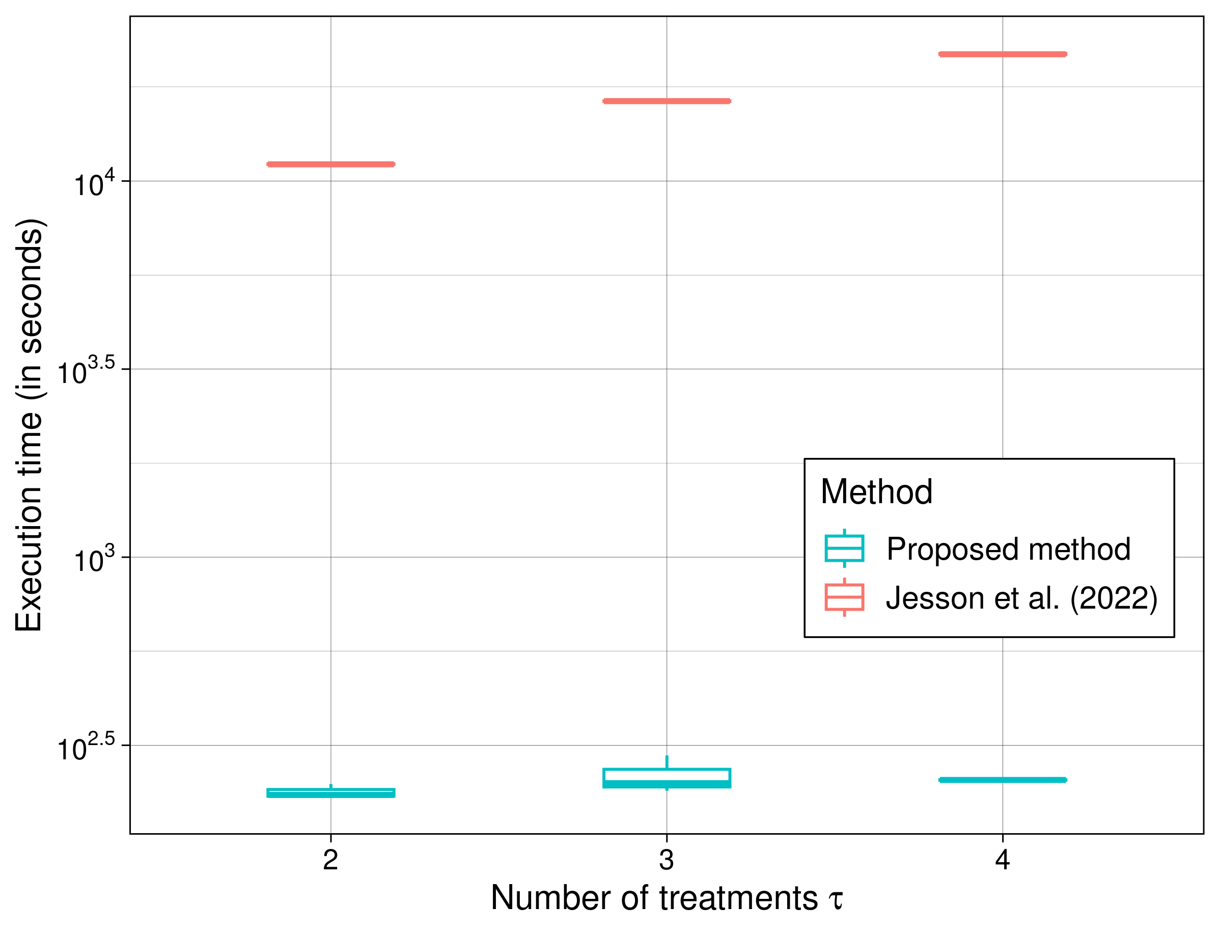
Figure 1: Boxplots of Execution Times (in Seconds) of the Proposed Method and [17] on 3 Monte-Carlo Samples. Sensitivity Analyses Were Performed for $m=2$, 3 and then 4 Values of Treatment of Interest $\tau$ (Setup from Table 2). The Times Do Not Include the Fine-Tuning Step of the Neural Networks.

Figure 2: Boxplots for the Upper and Lower Bounds of 95%-Level Confidence Intervals for 20 Monte-Carlo Samples. The Bounds from our Proposed Method Are in Blue While the Ones from the Concurrent Method [17] Are in Red. The True APO is Represented by Pink Squares. The Data Are Generated Using the Setup from Table 2, with an Estimated $\Gamma$ of 5.21.

4.3 Real Dataset Experiments

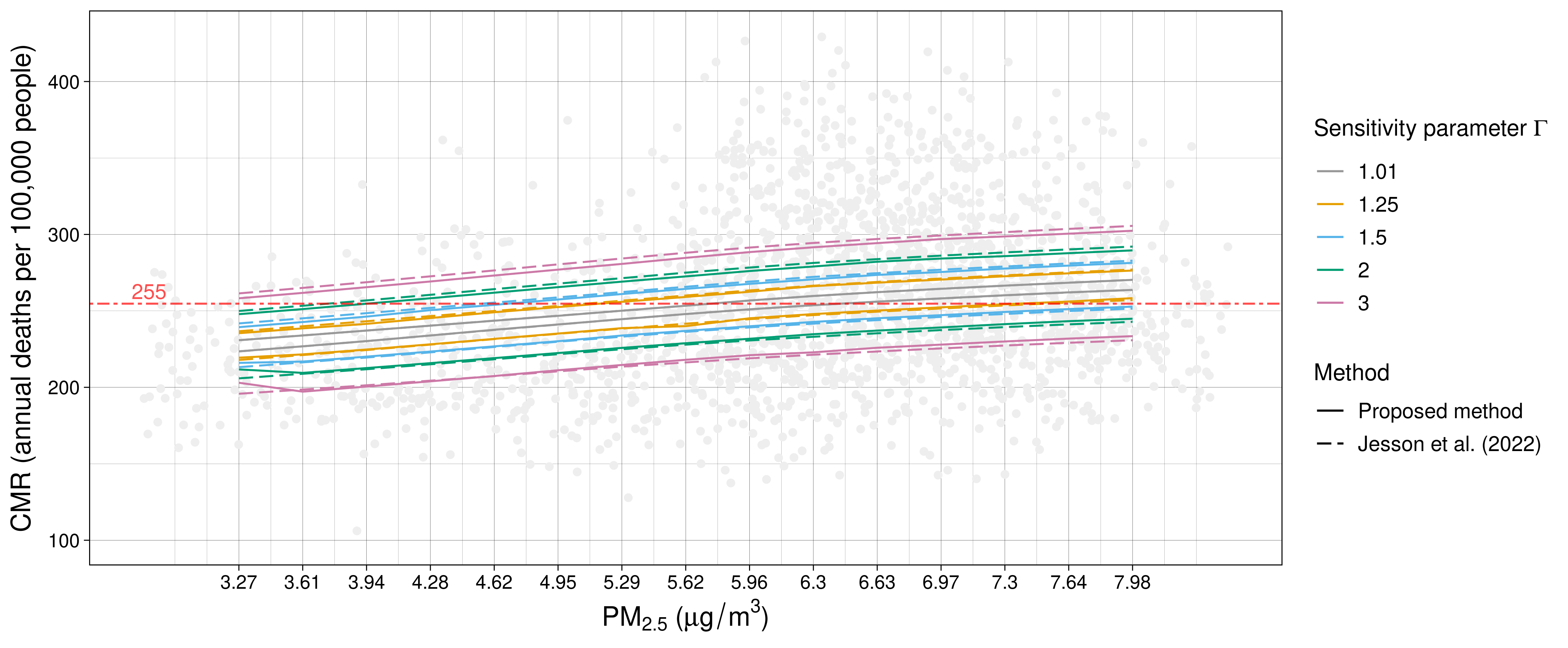
Figure 3: Sensitivity Analysis of the Real Dataset (95%-Level Confidence Intervals) with the Proposed Method and the One from [17] for 5 Values of $\Gamma$ and 15 Values of Exposition $\tau$ (PM2.5). The Red Dotted Line Corresponds to the Average CMR (255 Annual Deaths per 100,000 People). The Gray Points Are the Real Dataset With 84 Observations Removed to Improve Readability.

We further illustrate the behavior of our method on a publicly available dataset from the U.S. Environmental Protection Agency that studies the impact of annual PM2.5 level on cardiovascular mortality rate (CMR) in 2,132 U.S. counties between 1990 and 2010 [37]. PM2.5 fine particulate matter level corresponds to the continuous exposition $T$ and is measured in $\mu g/m^{3}$. CMR corresponds to the observed outcome $Y$ and is measured in annual deaths per 100,000 people. As in [3], we restrict the data to year 2010 to simplify the study and we consider 10 continuous variables as observed confounders $\mathbf{X}$. Finally, as in the simulated dataset, we remove 10% of extreme observations which leads to an effective sample size of $n=1918$. See Appendix B.6 for additional details on the preprocessing step.

In the following, the results are displayed for a user-defined range of values of the sensitivity parameter $\Gamma$. This is common in sensitivity analyses: in the continuous case, see [17]; in the binary case, see [39] or [7]. Another solution could be to set a certain threshold for the outcome, and to identify the lowest $\Gamma$ for which the threshold is in the CI. See Section 4.B. of [18] for a similar reasoning in the case of the Individual Treatment Effect (ITE), and [19] for other avenues to choose $\Gamma$. In any case, we do not estimate $\Gamma$ as in the previous subsection, as we do not have any external dataset with all possible confounders available.

After performing 2-fold cross-fitting on the data, 95%-level CIs are obtained with the proposed and concurrent methods for 15 different values of $\tau$ and 5 values of $\Gamma$ in Figure 3. First, as expected, we can observe that the confidence intervals grow as the sensitivity parameter $\Gamma$ increases. The gray curves, where $\Gamma=1.01$, correspond to results close to the $\mathbf{X}$-ignorability assumption, when $\Gamma=1$, i.e. results that could be obtained with estimator (2.1) from [20]. As $\Gamma$ increases, we deviate from $\mathbf{X}$-ignorability and assume that there are unobserved confounders. The more they have an effect on $T$, the more the uncertainty about the estimation of the treatment effect grows and the CIs become larger. Moreover, notice that, as the level of fine particles PM2.5 increases, there is a shift of the CIs towards greater values of the CMR. This observation supports the conclusion that cardiovascular mortality rate rises when the level of fine particles increases. However, if this result is significant when $\Gamma=1.01$, it is not true for larger values of $\Gamma$. Indeed, with $\Gamma=3$, the horizontal line representing the average CMR of 255 annual deaths per 100,000 people goes through all the CIs between 3.27 and 7.98 $\mu g/m^{3}$, and it could potentially be the true APO function. Thus, it would indicate no significant effect of PM2.5 level on the CMR. It is also immediately clear that the confidence intervals obtained with our method are smaller than the ones from [17]. Thus, with our method, a greater $\Gamma$ would be needed to move away from the hypothesis of effect of PM2.5 on CMR than with the concurrent method.

5 CONCLUSION AND FUTURE WORKS

We presented novel bounds for the APO after introducing a new continuous sensitivity model and leveraging a constraint on a likelihood ratio, derived confidence intervals from them, and showed that our algorithm outperforms existing methodologies in terms of computation times and sharpness. These results were demonstrated on a simulated dataset and real data from the U.S. Environmental Protection Agency. Additionally, we proposed doubly robust estimators of the bounds and performed an exploratory analysis on the variation of $\Gamma$ with respect to certain generation parameters of the dataset in appendix. To go further, it could be interesting to extend our method to the case where $T$ is multivariate, for example, to study drug antagonism or synergism. Moreover, in this article, we did not explain how to estimate the bounds for the CAPO from the data because it requires localizing the estimation around the covariates of interest, which is a case of high-dimensional regression. The estimation and interpretation of $\Gamma$ also requires additional investigation and is still an active domain of research. Finally, the suggested doubly robust estimators can be promising but more thorough examination is needed to improve their implementation.

6 DISCLOSURES

Jean-Baptiste Baitairian, Bernard Sebastien and Rana Jreich are Sanofi employees and may hold shares and/or stock options in the company. Agathe Guilloux is employed by INRIA. Sandrine Katsahian is employed by Université Paris-Cité and Assistance Publique – Hôpitaux de Paris (AP-HP). This work was supported by Sanofi and INRIA (Institut National de Recherche en Informatique et en Automatique).

References

Appendix A ADDITIONAL DEFINITIONS, ASSUMPTIONS, DETAILS AND PROOFS

In the following, we provide additional definitions used in the paper, along with proofs and their related assumptions.

A.1 Definitions

Definition A.1 corresponds to the sensitivity model that was considered in [17].

Definition A.1 (CMSM from [17]).

For a given treatment value $\tau\in\mathcal{T}$, for all $(\mathbf{x},y)\in\mathcal{X}\times\mathcal{Y}$, assuming $f(T=\tau|\mathbf{X}=\mathbf{x})$ is absolutely continuous with respect to $f(T=\tau|\mathbf{X}=\mathbf{x},Y(\tau)=y)$, there exists a sensitivity parameter $\Gamma\geq 1$ such that

$$\Gamma^{-1}\leq\frac{f(T=\tau|\mathbf{X}=\mathbf{x})}{f(T=\tau|\mathbf{X}=\mathbf{x},Y(\tau)=y)}\leq\Gamma.$$ (12)

Theorem 3.1 naturally leads to a conditional quantile. The following definition is the one we use in this paper.

Definition A.2 (Conditional quantile).

The generalized conditional quantile of order $\upsilon\in[0,1]$ of the distribution of $Y$ conditionally on $\mathbf{X}=\mathbf{x}$ and $T=t$ can be defined as:

$$Q(\upsilon;Y|\mathbf{X}=\mathbf{x},T=t)\overset{\mathrm{not.}}{=}q_{\upsilon}^{\mathbf{x},\mathbf{t}}\coloneq\inf\{q\in\mathbb{R},\,\mathbb{P}(Y\leq q|\mathbf{X}=\mathbf{x},T=t)>\upsilon\}.$$

A.2 Assumptions

Assumption A.3 ensures that the quotient in our sensitivity model (3) exists. Assumptions A.3 and A.4 are equivalent to assuming two by two absolute continuity of the densities. See Proposition 1 in [17] for another use of the absolute continuity assumption.

Assumption A.3 (Positivity and existence of the conditional densities for the treatment).

$\forall(\mathbf{x},\mathbf{u},t,y)\in\mathcal{X}\times\mathcal{U}\times\mathcal{T}\times\mathcal{Y},\,f(T=t|\mathbf{X}=\mathbf{x}),\,f(T=t|\mathbf{X}=\mathbf{x},Y(t)=y)\text{ and }f(T=t|\mathbf{X}=\mathbf{x},\mathbf{U}=\mathbf{u})$ exist and are positive. We will also assume that $\exists m_{f}>0,\,\forall(\mathbf{x},t)\in\mathcal{X}\times\mathcal{T},\,m_{f}\leq f(T=t|\mathbf{X}=\mathbf{x})$.

Assumption A.4 (Positivity and existence of the conditional densities for the outcome).

$\forall(\mathbf{x},t,y)\in\mathcal{X}\times\mathcal{T}\times\mathcal{Y},\,f(Y=y|\mathbf{X}=\mathbf{x})\text{ and }f(Y=y|\mathbf{X}=\mathbf{x},T=t)$ exist and are positive.

The following hypotheses concern the user-defined kernel. They are usual in nonparametric estimation.

Assumption A.5 (Kernel).

We assume that $K:\mathbb{R}\to\mathbb{R}_{+}$ is a symmetric and integrable kernel, with $\int_{-1}^{1}K(u)\,\mathrm{d}u=1$. We assume in addition that

1. $K$ is squared-integrable. In particular, $\exists M_{K^{2}}\in\mathbb{R},\,\int K^{2}(u)\,\mathrm{d}u\leq M_{K^{2}}<+\infty$.

2. $K$ is a kernel of order 1, i.e. $\exists M_{u^{2}K}\in\mathbb{R},\,\int u^{2}K(u)\,\mathrm{d}u\leq M_{u^{2}K}<+\infty$.

Assumption A.6 is classical in treatment effect estimation (see e.g., [20], [17], and [8]).

Assumption A.6.

The potential outcomes are bounded: $\exists M_{Y}\in\mathbb{R},\,|Y|\leq M_{Y}$.

The following assumptions are used in Theorem 3.2 to get bounds on the MSE of our estimators. For example, [1] uses similar hypotheses with kernels.

Assumption A.7.

For all $y\in\mathcal{Y}$ and $x\in\mathcal{X}$, the function $t\mapsto f(Y=y|\mathbf{X}=\mathbf{x},T=t)$ is $\mathcal{C}^{2}$ on $\mathcal{T}$. We also assume that, for a fixed treatment value $\tau\in\mathcal{T}$, for all $\mathbf{x}\in\mathcal{X}$, $\underset{y\in\mathcal{Y}}{\sup}|f(Y=y|\mathbf{X}=\mathbf{x},T=\tau)|=\lVert f\rVert_{\infty}<\infty$. In addition, there exists $M_{\partial^{2}f}\geq 0$ such that,

$$\forall(\mathbf{x},y,t)\in\mathcal{X}\times\mathcal{Y}\times\mathcal{T},\,\left|\pdv[order=2]{f}{T}(Y=y|\mathbf{X}=\mathbf{x},T=t)\right|\leq M_{\partial^{2}f}.$$

Assumption A.8.

For all $(\mathbf{x},y,\upsilon)$ in $\mathcal{X}\times\mathcal{Y}\times[0,1]$, the function $t\mapsto Q(\upsilon;Y|\mathbf{X}=\mathbf{x},T=t)$ is $\mathcal{C}^{2}$ on $\mathcal{T}$ and there exists $M_{\partial^{2}Q}\geq 0$ such that

$$\forall(\mathbf{x},t,\upsilon)\in\mathcal{X}\times\mathcal{T}\times[0,1],\,\left|\pdv[order=2]{Q}{T}(\upsilon;Y|\mathbf{X}=\mathbf{x},T=t)\right|\leq M_{\partial^{2}Q}.$$

Assumption A.9 is used to demonstrate the double robustness property in Proposition 3.3.

Assumption A.9.

For all $\mathbf{x}$ in $\mathcal{X}$, the function $t\mapsto\theta^{+}(t,\mathbf{x})=\mathbb{E}_{\mathbf{X}=\mathbf{x},T=t}[Y\Gamma^{\operatorname*{sign}(Y-q_{\gamma}^{\mathbf{x},t})}]$ is $\mathcal{C}^{2}$ on $\mathcal{T}$ and there exists $M_{\partial^{2}\theta^{+}}\geq 0$ such that

$$\forall(\mathbf{x},t)\in\mathcal{X}\times\mathcal{T},\,\left|\pdv[order=2]{\theta^{+}}{T}(t,\mathbf{x})\right|\leq M_{\partial^{2}\theta^{+}}.$$

A.3 Stabilized and Doubly Robust Estimations of the APO from [20]

The stabilized (or normalized) estimator from [20] can be written as:

$$\hat{\theta}^{\text{stab}}_{h}(\tau)=\sum_{i=1}^{n}\frac{K_{h}(T_{i}-\tau)Y_{i}}{\hat{f}(T=T_{i}|\mathbf{X}=\mathbf{X}_{i})}\Big{/}\sum_{j=1}^{n}\frac{K_{h}(T_{j}-\tau)}{\hat{f}(T=T_{j}|\mathbf{X}=\mathbf{X}_{j})}.$$ (13)

The doubly robust (or augmented) estimator from [20] can be written as:

$$\hat{\theta}^{\text{augm}}_{h}(\tau)=\hat{\eta}(\tau)+\frac{1}{n}\sum_{i=1}^{n}\frac{K_{h}(T_{i}-\tau)}{\hat{f}(T=T_{i}|\mathbf{X}=\mathbf{X}_{i})}(Y_{i}-\hat{\eta}(T_{i},\mathbf{X}_{i})),$$ (14)

where $\hat{\eta}(T_{i},\mathbf{X}_{i})$ is an estimator of $\operatorname*{\mathbb{E}}[Y|T=T_{i},\mathbf{X}=\mathbf{X}_{i}]$ and $\hat{\eta}(\tau)=\sum_{i=1}^{n}\hat{\eta}(\tau,\mathbf{X}_{i})/n$.

It is also possible to combine stabilization with double-robustness in one estimator. The estimator becomes:

$$\hat{\theta}^{\text{stab},\text{augm}}_{h}(\tau)=\hat{\eta}(\tau)+\frac{\sum_{i=1}^{n}\frac{K_{h}(T_{i}-\tau)}{\hat{f}(T=T_{i}|\mathbf{X}=\mathbf{X}_{i})}(Y_{i}-\hat{\eta}(T_{i},\mathbf{X}_{i}))}{\sum_{j=1}^{n}\frac{K_{h}(T_{j}-\tau)}{\hat{f}(T=T_{j}|\mathbf{X}=\mathbf{X}_{j})}},$$ (15)

Stabilization aims at reducing variance while double robustness ensures robustness to model misspecification: only $\hat{f}(T=T_{i}|\mathbf{X}=\mathbf{X}_{i})$ or $\hat{\eta}(\tau,\mathbf{X}_{i})$ needs to be correctly specified to ensure that the estimator is asymptotically unbiased.

A.4 Details for the Weight Function $w^{\star}$

We can rewrite the CAPO as

$$\theta(\tau,\mathbf{x}) \coloneq\mathbb{E}_{\mathbf{X}=\mathbf{x}}[Y(\tau)]$$

$$=\int yf(Y(\tau)=y|\mathbf{X}=\mathbf{x})\,\mathrm{d}y$$

$$=\int y\frac{f(Y(\tau)=y|\mathbf{X}=\mathbf{x})}{f(Y=y|\mathbf{X}=\mathbf{x},T=\tau)}f(Y=y|\mathbf{X}=\mathbf{x},T=\tau)\,\mathrm{d}y\quad\text{by Assumption~{}\ref{ass:positivity_cond_outcome}}$$

$$=\mathbb{E}_{\mathbf{X}=\mathbf{x},T=\tau}[Yw^{\star}(Y,\mathbf{x},\tau)],$$

where, for all $(\mathbf{x},t,y)\in\mathcal{X}\times\mathcal{T}\times\mathcal{Y}$, the likelihood ratio $w^{\star}$ is defined as

$$w^{\star}(y,\mathbf{x},t)=\frac{f\bigl{(}Y(t)=y\big{|}\mathbf{X}=\mathbf{x}\bigr{)}}{f\bigl{(}Y=y\big{|}\mathbf{X}=\mathbf{x},T=t\bigr{)}}.$$

Moreover, for all $(\mathbf{x},t)\in\mathcal{X}\times\mathcal{T}$,

$$\mathbb{E}_{\mathbf{X}=\mathbf{x},T=t}[w^{\star}(Y,\mathbf{x},t)] =\int\frac{f\bigl{(}Y(t)=y\big{|}\mathbf{X}=\mathbf{x}\bigr{)}}{f\bigl{(}Y=y|\mathbf{X}=\mathbf{x},T=t\bigr{)}}f\bigl{(}Y=y\big{|}\mathbf{X}=\mathbf{x},T=t\bigr{)}\,\mathrm{d}y$$

$$=\int f\bigl{(}Y(t)=y\big{|}\mathbf{X}=\mathbf{x}\bigr{)}\,\mathrm{d}y=1,$$

which leads to Equation (4).

A.5 All Bounds for the CAPO and APO

A.5.1 Bounds for the CAPO

From the proof of Theorem 3.1, we can get the true bounds for the CAPO:

$$\theta^{-}(\tau,\mathbf{x}) =\eta(\tau,\mathbf{x})+\frac{2\gamma-1}{\gamma}\mathbb{E}_{\mathbf{X}=\mathbf{x},T=\tau}\Bigl{[}Y-\eta(\tau,\mathbf{x})\Big{|}Y\leq q_{1-\gamma}^{\mathbf{x},\tau}\Bigr{]}$$ (16)

$$=\eta(\tau,\mathbf{x})+\mathbb{E}_{\mathbf{X}=\mathbf{x},T=\tau}\Bigl{[}(Y-\eta(\tau,\mathbf{x}))\Gamma^{-\operatorname*{sign}(Y-q_{1-\gamma}^{\mathbf{x},\tau})}\Bigr{]}$$ (17)

and

$$\theta^{+}(\tau,\mathbf{x}) =\eta(\tau,\mathbf{x})+\frac{2\gamma-1}{\gamma}\mathbb{E}_{\mathbf{X}=\mathbf{x},T=\tau}\Bigl{[}Y-\eta(\tau,\mathbf{x})\Big{|}Y>q_{\gamma}^{\mathbf{x},\tau}\Bigr{]}$$ (18)

$$=\eta(\tau,\mathbf{x})+\mathbb{E}_{\mathbf{X}=\mathbf{x},T=\tau}\Bigl{[}(Y-\eta(\tau,\mathbf{x}))\Gamma^{\operatorname*{sign}(Y-q_{\gamma}^{\mathbf{x},\tau})}\Bigr{]}$$ (19)

where $\gamma=\Gamma/(1+\Gamma)$ and $q_{\upsilon}^{\mathbf{x},\tau}=Q(\upsilon;Y|\mathbf{X}=\mathbf{x},T=\tau)$.

In subsection 3.3, the kernelized versions of the bounds are given by

$$\theta_{h}^{-}(\tau,\mathbf{x}) =\eta(\tau,\mathbf{x})+\frac{2\gamma-1}{\gamma}\mathbb{E}_{\mathbf{X}=\mathbf{x}}\biggl{[}\frac{K_{h}(T-\tau)}{f(T|\mathbf{X}=\mathbf{x})}(Y-\eta(\tau,\mathbf{x}))\bigg{|}Y\leq q_{1-\gamma}^{\mathbf{x},T}\biggr{]}$$ (20)

$$=\eta(\tau,\mathbf{x})+\mathbb{E}_{\mathbf{X}=\mathbf{x}}\biggl{[}\frac{K_{h}(T-\tau)}{f(T|\mathbf{X}=\mathbf{x})}(Y-\eta(\tau,\mathbf{x}))\Gamma^{-\operatorname*{sign}(Y-q_{1-\gamma}^{\mathbf{x},T})}\biggr{]}$$ (21)

and

$$\theta_{h}^{+}(\tau,\mathbf{x}) =\eta(\tau,\mathbf{x})+\frac{2\gamma-1}{\gamma}\mathbb{E}_{\mathbf{X}=\mathbf{x}}\biggl{[}\frac{K_{h}(T-\tau)}{f(T|\mathbf{X}=\mathbf{x})}(Y-\eta(\tau,\mathbf{x}))\bigg{|}Y>q_{\gamma}^{\mathbf{x},T}\biggr{]}$$ (22)

$$=\eta(\tau,\mathbf{x})+\mathbb{E}_{\mathbf{X}=\mathbf{x}}\biggl{[}\frac{K_{h}(T-\tau)}{f(T|\mathbf{X}=\mathbf{x})}(Y-\eta(\tau,\mathbf{x}))\Gamma^{\operatorname*{sign}(Y-q_{\gamma}^{\mathbf{x},T})}\biggr{]}$$ (23)

where $K_{h}$ is defined as in Equation (2.1).

A.5.2 Bounds for the APO

From the proof of Theorem 3.1 and the relation $\theta(\tau)=\operatorname*{\mathbb{E}}[\theta(\tau,\mathbf{X})]$, we can get the true bounds for the APO:

$$\theta^{-}(\tau) =\eta(\tau)+\frac{2\gamma-1}{\gamma}\operatorname*{\mathbb{E}}\biggl{[}\mathbb{E}_{\mathbf{X},T=\tau}\Bigl{[}Y-\eta(\tau,\mathbf{X})\Big{|}Y\leq q_{1-\gamma}^{\mathbf{X},\tau}\Bigr{]}\biggr{]}$$ (24)

$$=\eta(\tau)+\operatorname*{\mathbb{E}}\biggl{[}\mathbb{E}_{\mathbf{X},T=\tau}\Bigl{[}(Y-\eta(\tau,\mathbf{X}))\Gamma^{-\operatorname*{sign}(Y-q_{1-\gamma}^{\mathbf{X},\tau})}\Bigr{]}\biggr{]}$$ (25)

and

$$\theta^{+}(\tau) =\eta(\tau)+\frac{2\gamma-1}{\gamma}\operatorname*{\mathbb{E}}\biggl{[}\mathbb{E}_{\mathbf{X},T=\tau}\Bigl{[}Y-\eta(\tau,\mathbf{X})\Big{|}Y>q_{\gamma}^{\mathbf{X},\tau}\Bigr{]}\biggr{]}$$ (26)

$$=\eta(\tau)+\operatorname*{\mathbb{E}}\biggl{[}\mathbb{E}_{\mathbf{X},T=\tau}\Bigl{[}(Y-\eta(\tau,\mathbf{X}))\Gamma^{\operatorname*{sign}(Y-q_{\gamma}^{\mathbf{X},\tau})}\Bigr{]}\biggr{]},$$ (27)

where $\eta(\tau)=\operatorname*{\mathbb{E}}[\eta(\tau,\mathbf{X})]$, $\gamma=\Gamma/(1+\Gamma)$ and $q_{\upsilon}^{\mathbf{X},\tau}=Q(\upsilon;Y|\mathbf{X},T=\tau)$.

In subsection 3.3, the kernelized versions of the bounds are given by

$$\theta_{h}^{-}(\tau) =\eta(\tau)+\frac{2\gamma-1}{\gamma}\operatorname*{\mathbb{E}}\biggl{[}\mathbb{E}\biggl{[}\frac{K_{h}(T-\tau)}{f(T|\mathbf{X})}(Y-\eta(\tau,\mathbf{X}))\bigg{|}\mathbf{X},Y\leq q_{1-\gamma}^{\mathbf{X},T}\biggr{]}\biggr{]}$$ (28)

$$=\eta(\tau)+\operatorname*{\mathbb{E}}\biggl{[}\frac{K_{h}(T-\tau)}{f(T|\mathbf{X})}(Y-\eta(\tau,\mathbf{X}))\Gamma^{-\operatorname*{sign}(Y-q_{1-\gamma}^{\mathbf{X},T})}\biggr{]}$$ (29)

and

$$\theta_{h}^{+}(\tau) =\eta(\tau)+\frac{2\gamma-1}{\gamma}\operatorname*{\mathbb{E}}\biggl{[}\mathbb{E}\biggl{[}\frac{K_{h}(T-\tau)}{f(T|\mathbf{X})}(Y-\eta(\tau,\mathbf{X}))\bigg{|}\mathbf{X},Y>q_{\gamma}^{\mathbf{X},T}\biggr{]}\biggr{]}$$ (30)

$$=\eta(\tau)+\operatorname*{\mathbb{E}}\biggl{[}\frac{K_{h}(T-\tau)}{f(T|\mathbf{X})}(Y-\eta(\tau,\mathbf{X}))\Gamma^{\operatorname*{sign}(Y-q_{\gamma}^{\mathbf{X},T})}\biggr{]},$$ (31)

where $K_{h}$ is defined as in Equation (2.1).

By defining $\mathcal{I}_{\mathcal{D_{-}}}=\{i\in[\![1,n]\!]\,;\,Y_{i}\leq q_{1-\gamma}^{\mathbf{X}_{i},T_{i}}\}$ of cardinality $n_{-}$, and $\mathcal{I}_{\mathcal{D_{+}}}=\{i\in[\![1,n]\!]\,;\,Y_{i}>q_{\gamma}^{\mathbf{X}_{i},T_{i}}\}$ of cardinality $n_{+}$, we can obtain estimators of $\theta_{h}^{-}(\tau)$ and $\theta_{h}^{+}(\tau)$ as follows, using Equations (28) and (30):

$$\tilde{\theta}_{h}^{-}(\tau)=\tilde{\eta}(\tau)+\frac{2\gamma-1}{\gamma n_{-}}\sum_{i\in\mathcal{I}_{\mathcal{D_{-}}}}\frac{K_{h}(T_{i}-\tau)}{f(T_{i}|\mathbf{X}_{i})}(Y_{i}-\eta(T_{i},\mathbf{X}_{i}))$$ (32)

and

$$\tilde{\theta}_{h}^{+}(\tau)=\tilde{\eta}(\tau)+\frac{2\gamma-1}{\gamma n_{+}}\sum_{i\in\mathcal{I}_{\mathcal{D_{+}}}}\frac{K_{h}(T_{i}-\tau)}{f(T_{i}|\mathbf{X}_{i})}(Y_{i}-\eta(T_{i},\mathbf{X}_{i})),$$ (33)

where $\tilde{\eta}(\tau)=\frac{1}{n}\sum_{i=1}^{n}\eta(\tau,\mathbf{X}_{i})$.

Using Equations (29) and (31), we can also get estimators via

$$\tilde{\theta}_{h}^{-}(\tau)=\tilde{\eta}(\tau)+\frac{1}{n}\sum_{i=1}^{n}\frac{K_{h}(T_{i}-\tau)(Y_{i}-\eta(T_{i},\mathbf{X}_{i}))}{f(T_{i}|\mathbf{X}_{i})}\Gamma^{-\operatorname*{sign}\left(Y_{i}-q_{1-\gamma}^{\mathbf{X}_{i},T_{i}}\right)}$$ (34)

and

$$\tilde{\theta}_{h}^{+}(\tau)=\tilde{\eta}(\tau)+\frac{1}{n}\sum_{i=1}^{n}\frac{K_{h}(T_{i}-\tau)(Y_{i}-\eta(T_{i},\mathbf{X}_{i}))}{f(T_{i}|\mathbf{X}_{i})}\Gamma^{\operatorname*{sign}\left(Y_{i}-q_{\gamma}^{\mathbf{X}_{i},T_{i}}\right)},$$ (35)

where $\tilde{\eta}(\tau)=\frac{1}{n}\sum_{i=1}^{n}\eta(\tau,\mathbf{X}_{i})$.

In practice, we use stabilized versions of our estimators to reduce their variance. Thus, Equations (32) and (33) become

$$\tilde{\theta}_{h}^{-,\mathrm{stab}}(\tau)=\tilde{\eta}(\tau)+\frac{2\gamma-1}{\gamma}\cdot\frac{\sum_{i\in\mathcal{I}_{\mathcal{D_{-}}}}\frac{K_{h}(T_{i}-\tau)}{f(T_{i}|\mathbf{X}_{i})}(Y_{i}-\eta(T_{i},\mathbf{X}_{i}))}{\sum_{j\in\mathcal{I}_{\mathcal{D_{-}}}}\frac{K_{h}(T_{j}-\tau)}{f(T_{j}|\mathbf{X}_{j})}}$$ (36)

and

$$\tilde{\theta}_{h}^{+,\mathrm{stab}}(\tau)=\tilde{\eta}(\tau)+\frac{2\gamma-1}{\gamma}\cdot\frac{\sum_{i\in\mathcal{I}_{\mathcal{D_{+}}}}\frac{K_{h}(T_{i}-\tau)}{f(T_{i}|\mathbf{X}_{i})}(Y_{i}-\eta(T_{i},\mathbf{X}_{i}))}{\sum_{j\in\mathcal{I}_{\mathcal{D_{+}}}}\frac{K_{h}(T_{j}-\tau)}{f(T_{j}|\mathbf{X}_{j})}},$$ (37)

and Equations (34) and (35) become

$$\tilde{\theta}_{h}^{-,\mathrm{stab}}(\tau)=\tilde{\eta}(\tau)+\frac{\sum_{i=1}^{n}\frac{K_{h}(T_{i}-\tau)(Y_{i}-\eta(T_{i},\mathbf{X}_{i}))}{f(T_{i}|\mathbf{X}_{i})}\Gamma^{-\operatorname*{sign}\left(Y_{i}-q_{1-\gamma}^{\mathbf{X}_{i},T_{i}}\right)}}{\sum_{j=1}^{n}\frac{K_{h}(T_{j}-\tau)}{f(T_{j}|\mathbf{X}_{j})}\Gamma^{-\operatorname*{sign}\left(Y_{j}-q_{1-\gamma}^{\mathbf{X}_{j},T_{j}}\right)}}$$ (38)

and

$$\tilde{\theta}_{h}^{+,\mathrm{stab}}(\tau)=\tilde{\eta}(\tau)+\frac{\sum_{i=1}^{n}\frac{K_{h}(T_{i}-\tau)(Y_{i}-\eta(T_{i},\mathbf{X}_{i}))}{f(T_{i}|\mathbf{X}_{i})}\Gamma^{\operatorname*{sign}\left(Y_{i}-q_{\gamma}^{\mathbf{X}_{i},T_{i}}\right)}}{\sum_{j=1}^{n}\frac{K_{h}(T_{j}-\tau)}{f(T_{j}|\mathbf{X}_{j})}\Gamma^{\operatorname*{sign}\left(Y_{j}-q_{\gamma}^{\mathbf{X}_{j},T_{j}}\right)}},$$ (39)

where $\tilde{\eta}(\tau)=\frac{1}{n}\sum_{i=1}^{n}\eta(\tau,\mathbf{X}_{i})$.

A.6 Percentile Bootstrap Method

From the bounds obtained in the previous subsection, we can derive confidence intervals via the percentile bootstrap, as done in [39]. Figure 4 gives an intuitive visualization of this method.

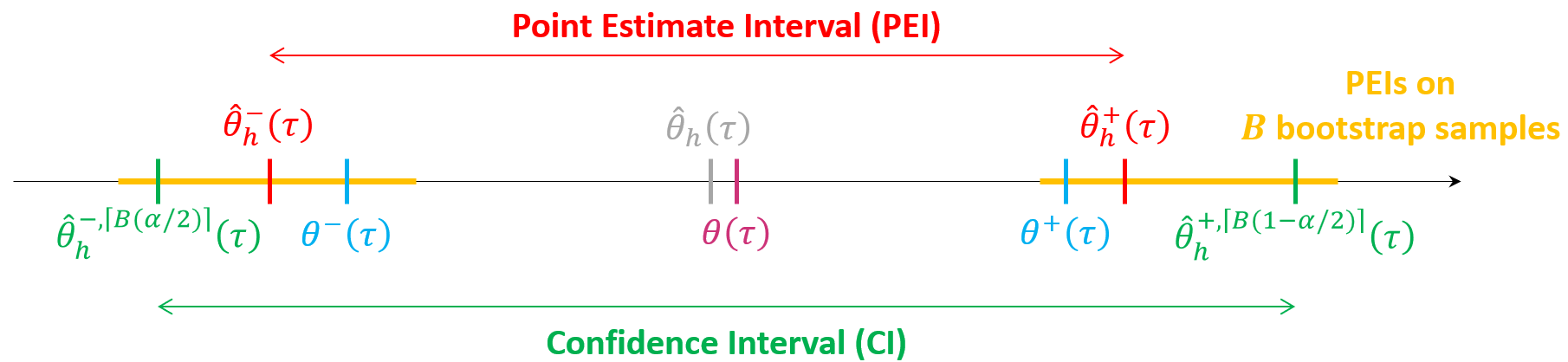
Figure 4: Percentile Bootstrap Method

In Figure 4, the true unknown APO is represented in violet. The APO estimated via Equation (2.1) is in gray. The two true bounds on the APO from Equation (9) are represented in blue. If we estimate these bounds on the whole dataset, we can get the Point Estimate Interval in red. Instead of using the whole dataset, if we compute the PEI on $B$ bootstrap samples and then take the quantiles of order $\alpha/2$ and $1-\alpha/2$ of, respectively, the lower and upper bounds, we can get a $(1-\alpha)$-level confidence interval in green. The ranges of lower bounds and upper bounds on the $B$ bootstrap samples are represented in yellow.

As mentioned in the main text, a two-sided $(1-\alpha)$-CI for the set $\bigl{[}\theta^{-}_{h}(\tau),\theta^{+}_{h}(\tau)\bigr{]}$ can be obtained after intersecting two one-sided $(1-\alpha/2)$-CIs for the lower and the upper bounds. Indeed, by the union bound,

$$\mathbb{P}\Bigl{(}\bigl{[}\theta_{h}^{-}(\tau),\,\theta_{h}^{+}(\tau)\bigr{]}\not\subset\bigl{[}\hat{\theta}_{h}^{-,\lceil B(\alpha/2)\rceil}(\tau),\,\hat{\theta}_{h}^{+,\lceil B(1-\alpha/2)\rceil}(\tau)\bigr{]}\Bigr{)}$$

$$=\mathbb{P}\Bigl{(}\bigl{\{}\theta_{h}^{-}(\tau)<\hat{\theta}_{h}^{-,\lceil B(\alpha/2)\rceil}(\tau)\bigr{\}}\cup\bigl{\{}\hat{\theta}_{h}^{+,\lceil B(1-\alpha/2)\rceil}(\tau)<\theta_{h}^{+}(\tau)\bigr{\}}\Bigr{)}$$

$$\leq\mathbb{P}\Bigl{(}\theta_{h}^{-}(\tau)<\hat{\theta}_{h}^{-,\lceil B(\alpha/2)\rceil}(\tau)\Bigr{)}+\mathbb{P}\Bigl{(}\hat{\theta}_{h}^{+,\lceil B(1-\alpha/2)\rceil}(\tau)<\theta_{h}^{+}(\tau)\Bigr{)}$$

$$\leq\frac{\alpha}{2}+\frac{\alpha}{2}=\alpha.$$

Therefore,

$$\mathbb{P}\Bigl{(}\bigl{[}\theta_{h}^{-}(\tau),\,\theta_{h}^{+}(\tau)\bigr{]}\subset\bigl{[}\hat{\theta}_{h}^{-,\lceil B(\alpha/2)\rceil}(\tau),\,\hat{\theta}_{h}^{+,\lceil B(1-\alpha/2)\rceil}(\tau)\bigr{]}\Bigr{)}\geq 1-\alpha.$$

A.7 Proof of Proposition 2.2

Under Assumptions A.3 and A.4, simple computations show that the ratio considered in the sensitivity model from [17] (see Definition A.1 or their Definition 1) satisfies, for a fixed treatment value $\tau\in\mathcal{T}$,

$$\forall(\mathbf{x},y)\in\mathcal{X}\times\mathcal{Y},\,\frac{f\bigl{(}T=\tau\big{|}\mathbf{X}=\mathbf{x},Y(\tau)=y\bigr{)}}{f\bigl{(}T=\tau\big{|}\mathbf{X}=\mathbf{x}\bigr{)}}=\frac{f\bigl{(}Y(\tau)=y\big{|}\mathbf{X}=\mathbf{x},T=\tau\bigr{)}}{f\bigl{(}Y(\tau)=y\big{|}\mathbf{X}=\mathbf{x}\bigr{)}}$$ (40)

by Bayes’ theorem. Now, notice that

$$\forall(\mathbf{x},\mathbf{u})\in\mathcal{X}\times\mathcal{U},\,\upsilon(\mathbf{u},\mathbf{x},\tau)\coloneq\frac{f\bigl{(}\mathbf{U}=\mathbf{u}\big{|}\mathbf{X}=\mathbf{x}\bigr{)}}{f\bigl{(}\mathbf{U}=\mathbf{u}\big{|}\mathbf{X}=\mathbf{x},T=\tau\bigr{)}}=\frac{f\bigl{(}T=\tau\big{|}\mathbf{X}=\mathbf{x}\bigr{)}}{f\bigl{(}T=\tau\big{|}\mathbf{X}=\mathbf{x},\mathbf{U}=\mathbf{u}\bigr{)}}$$

is in $[\Gamma^{-1},\Gamma]$ under the CMSM from Definition 2.1. Moreover, $(\mathbf{X},\mathbf{U})$-ignorability implies that

$$f\bigl{(}Y(\tau)=y\big{|}\mathbf{X}=\mathbf{x}\bigr{)} =\int_{\mathcal{U}}f\bigl{(}Y(\tau)=y,\mathbf{U}=\mathbf{u}\big{|}\mathbf{X}=\mathbf{x}\bigr{)}\,\mathrm{d}\mathbf{u}$$

$$=\int_{\mathcal{U}}f\bigl{(}Y(\tau)=y\big{|}\mathbf{X}=\mathbf{x},\mathbf{U}=\mathbf{u}\bigr{)}f\bigl{(}\mathbf{U}=\mathbf{u}\big{|}\mathbf{X}=\mathbf{x}\bigr{)}\,\mathrm{d}\mathbf{u}$$

$$=\int_{\mathcal{U}}f\bigl{(}Y(\tau)=y\big{|}\mathbf{X}=\mathbf{x},\mathbf{U}=\mathbf{u},T=\tau\bigr{)}f\bigl{(}\mathbf{U}=\mathbf{u}\big{|}\mathbf{X}=\mathbf{x},T=\tau\bigr{)}\upsilon(\mathbf{u},\mathbf{x},\tau)\,\mathrm{d}\mathbf{u}.$$

Therefore, by Bayes’ theorem and as $\upsilon(\mathbf{u},\mathbf{x},\tau)$ is in $[\Gamma^{-1},\Gamma]$ for all $\mathbf{x}$ and $\mathbf{u}$,

$$\Gamma^{-1}\int_{\mathcal{U}}f\bigl{(}Y(\tau)=y,\mathbf{U}=\mathbf{u}\big{|}\mathbf{X}=\mathbf{x},T=\tau\bigr{)}\,\mathrm{d}\mathbf{u}\leq f\bigl{(}Y(\tau)=y\big{|}\mathbf{X}=\mathbf{x}\bigr{)}\leq\Gamma\int_{\mathcal{U}}f\bigl{(}Y(\tau)=y,\mathbf{U}=\mathbf{u}\big{|}\mathbf{X}=\mathbf{x},T=\tau\bigr{)}\,\mathrm{d}\mathbf{u}$$

$$\Rightarrow\Gamma^{-1}f\bigl{(}Y(\tau)=y\big{|}\mathbf{X}=\mathbf{x},T=\tau\bigr{)}\leq f\bigl{(}Y(\tau)=y\big{|}\mathbf{X}=\mathbf{x}\bigr{)}\leq\Gamma f\bigl{(}Y(\tau)=y\big{|}\mathbf{X}=\mathbf{x},T=\tau\bigr{)}$$

$$\Rightarrow\Gamma^{-1}\leq\frac{f\bigl{(}Y(\tau)=y\big{|}\mathbf{X}=\mathbf{x}\bigr{)}}{f\bigl{(}Y(\tau)=y\big{|}\mathbf{X}=\mathbf{x},T=\tau\bigr{)}}\leq\Gamma$$

Finally, using Equation (40), we just proved that our sensitivity model implies the one from [17].

A.8 Proof of Theorem 3.1

The proof focuses on the lower bound for the CAPO $\theta^{-}(\tau,\mathbf{x})$ but a similar reasoning can be used for the upper bound $\theta^{+}(\tau,\mathbf{x})$.

Notice that the minimization problem (6) can be written:

$$\theta^{-}(\tau,\mathbf{x}) =\eta(\tau,\mathbf{x})+\inf_{w\in\mathcal{W}^{\star}_{\tau}}\mathbb{E}_{\mathbf{X}=\mathbf{x},T=\tau}\bigl{[}\bigl{(}Y-\eta(\tau,\mathbf{x})\bigr{)}w(Y,\mathbf{x},\tau)\bigr{]}$$

$$=\Gamma^{-1}\eta(\tau,\mathbf{x})+(1-\Gamma^{-1})\underset{w\in\mathcal{W}^{\star}_{\tau}}{\inf}\mathbb{E}_{\mathbf{X}=\mathbf{x},T=\tau}\Biggl{[}Y\frac{w(Y,\mathbf{x},\tau)-\Gamma^{-1}}{1-\Gamma^{-1}}\Biggr{]}$$

Now, rewrite

$$\mathbb{E}_{\mathbf{X}=\mathbf{x},T=\tau}\Biggl{[}Y\frac{w(Y,\mathbf{x},\tau)-\Gamma^{-1}}{1-\Gamma^{-1}}\Biggr{]} =\int y\frac{w(y,\mathbf{x},\tau)-\Gamma^{-1}}{1-\Gamma^{-1}}f(Y=y|\mathbf{X}=\mathbf{x},T=\tau)\,\mathrm{d}y$$

$$=\int yg(y,\mathbf{x},\tau)f(Y=y|\mathbf{X}=\mathbf{x},T=\tau)\,\mathrm{d}y$$

where $g(y,\mathbf{x},\tau)\coloneq(w(y,\mathbf{x},\tau)-\Gamma^{-1})/(1-\Gamma^{-1})$ is a density ratio because $f(Y=y|\mathbf{X}=\mathbf{x},T=\tau)g(y,\mathbf{x},\tau)$ is a density. Indeed,

$$\int f(Y=y|\mathbf{X}=\mathbf{x},T=\tau)g(y,\mathbf{x},\tau)\,\mathrm{d}y =\frac{1}{1-\Gamma^{-1}}\int f(Y=y|\mathbf{X}=\mathbf{x},T=\tau)\left(\frac{f(Y(\tau)=y|\mathbf{X}=\mathbf{x})}{f(Y=y|\mathbf{X}=\mathbf{x},T=\tau)}-\Gamma^{-1}\right)\,\mathrm{d}y$$

$$=\frac{1}{1-\Gamma^{-1}}\int f(Y=y|\mathbf{X}=\mathbf{x},T=\tau)-\Gamma^{-1}f(Y(\tau)=y|\mathbf{X}=\mathbf{x})\,\mathrm{d}y$$

$$=\frac{1}{1-\Gamma^{-1}}-\frac{\Gamma^{-1}}{1-\Gamma^{-1}}=1$$

and, as $w\in\mathcal{W}^{\star}(\tau)$,

$$g(y,\mathbf{x},\tau)=\frac{1}{1-\Gamma^{-1}}\left(w(y,\mathbf{x},\tau)-\Gamma^{-1}\right)\in[0,\Gamma+1]=[0,(1-\gamma)^{-1}],$$

so $f(Y=y|\mathbf{X}=\mathbf{x},T=\tau)g(y,\mathbf{x},\tau)$ is nonnegative.

Therefore,

$$\underset{w\in\mathcal{W}^{\star}_{\tau}}{\inf}\mathbb{E}_{\mathbf{X}=\mathbf{x},T=\tau}\Biggl{[}Y\frac{w(Y,\mathbf{x},\tau)-\Gamma^{-1}}{1-\Gamma^{-1}}\Biggr{]}=\underset{g(Y,\mathbf{x},\tau)\leq\frac{1}{1-\gamma}}{\inf}\mathbb{E}_{\mathbf{X}=\mathbf{x},T=\tau}[Yg(Y,\mathbf{x},\tau)].$$

The “Fenchel-Moreau-Rockafellar” dual representation of the Expected Shortfall $\mathrm{ES}_{1-\gamma}(Y)\coloneq\mathbb{E}_{\mathbf{X}=\mathbf{x},T=\tau}[-Y|Y\leq q_{1-\gamma}^{\mathbf{x},\tau}]$ gives (e.g., see [12]):

$$\mathrm{ES}_{1-\gamma}(Y)=\underset{g(Y,\mathbf{x},\tau)\leq\frac{1}{1-\gamma}}{\sup}\mathbb{E}_{\mathbf{X}=\mathbf{x},T=\tau}[-Yg(Y,\mathbf{x},\tau)]=-\underset{g(Y,\mathbf{x},\tau)\leq\frac{1}{1-\gamma}}{\inf}\mathbb{E}_{\mathbf{X}=\mathbf{x},T=\tau}[Yg(Y,\mathbf{x},\tau)]$$

This leads to the following equality:

$$\theta^{-}(\tau,\mathbf{x})=\Gamma^{-1}\eta(\tau,\mathbf{x})+(\Gamma^{-1}-1)\mathbb{E}_{\mathbf{X}=\mathbf{x},T=\tau}[-Y|Y\leq q_{1-\gamma}^{\mathbf{x},\tau}].$$ (41)

Finally, to get a dependence only in $\gamma$, we can rewrite the lower bound for the CAPO:

$$\theta^{-}(\tau,\mathbf{x}) =\Gamma^{-1}\eta(\tau,\mathbf{x})+(\Gamma^{-1}-1)\mathbb{E}_{\mathbf{X}=\mathbf{x},T=\tau}[-Y|Y\leq q_{1-\gamma}^{\mathbf{x},\tau}]$$

$$=\frac{1-\gamma}{\gamma}\eta(\tau,\mathbf{x})+\frac{1-2\gamma}{\gamma}\mathbb{E}_{\mathbf{X}=\mathbf{x},T=\tau}[-Y|Y\leq q_{1-\gamma}^{\mathbf{x},\tau}]$$

$$=\eta(\tau,\mathbf{x})+\frac{1-2\gamma}{\gamma}\mathbb{E}_{\mathbf{X}=\mathbf{x},T=\tau}[-Y|Y\leq q_{1-\gamma}^{\mathbf{x},\tau}]+\frac{1-2\gamma}{\gamma}\mathbb{E}_{\mathbf{X}=\mathbf{x},T=\tau}[\eta(\tau,\mathbf{x})|Y\leq q_{1-\gamma}^{\mathbf{x},\tau}]$$

$$=\eta(\tau,\mathbf{x})+\frac{2\gamma-1}{\gamma}\mathbb{E}_{\mathbf{X}=\mathbf{x},T=\tau}[Y-\eta(\tau,\mathbf{x})|Y\leq q_{1-\gamma}^{\mathbf{x},\tau}].$$

Similarly, the upper bound for the CAPO is given by

$$\theta^{+}(\tau,\mathbf{x})=\eta(\tau,\mathbf{x})+\frac{2\gamma-1}{\gamma}\mathbb{E}_{\mathbf{X}=\mathbf{x},T=\tau}[Y-\eta(\tau,\mathbf{x})|Y>q_{\gamma}^{\mathbf{x},\tau}].$$

As the proof relies on the “Fenchel-Moreau-Rockafellar” dual representation, which is an optimum, the interval $[\theta^{-}(\tau,\mathbf{x}),\theta^{+}(\tau,\mathbf{x})]$ is also sharp under the CMSM.

A.9 Alternative Proof of the Bounds $\theta^{-}(\tau,\mathbf{x})$ and $\theta^{+}(\tau,\mathbf{x})$ from Theorem 3.1

In this alternative proof of the bounds for the CAPO, we leverage the constraint on the weight function from Equation (4), which reminds the Quantile Balancing condition from [7] in the binary treatment case.

We first show that the minimizer and maximizer of the optimization problems (6) and (7) are

$$w^{-}(Y,\mathbf{x},\tau)=\Gamma^{-\operatorname*{sign}\left(Y-Q\left(1-\gamma;\,Y|\mathbf{X}=\mathbf{x},T=\tau\right)\right)}\text{ and }w^{+}(Y,\mathbf{x},\tau)=\Gamma^{\operatorname*{sign}\left(Y-Q\left(\gamma;\,Y|\mathbf{X}=\mathbf{x},T=\tau\right)\right)},$$

where $\operatorname*{sign}(\cdot)$ is the sign function.

We focus on the maximization problem (7). First, $w^{+}(Y,\mathbf{x},\tau)$ fulfills Equation (4) because

$$\mathbb{E}_{\mathbf{X}=\mathbf{x},T=\tau}[w^{+}(Y,\mathbf{x},\tau)] =\int_{\mathcal{Y}}\Gamma^{\operatorname*{sign}(y-Q(\gamma;Y|\mathbf{X}=\mathbf{x},T=\tau))}f(Y=y|\mathbf{X}=\mathbf{x},T=\tau)\,\mathrm{d}y$$

$$=\Gamma\int_{\mathcal{Y}}\mathbb{1}(y>Q(\gamma;Y|\mathbf{X}=\mathbf{x},T=\tau))f(Y=y|\mathbf{X}=\mathbf{x},T=\tau)\,\mathrm{d}y$$

$$\quad+\Gamma^{-1}\int_{\mathcal{Y}}\mathbb{1}(y\leq Q(\gamma;Y|\mathbf{X}=\mathbf{x},T=\tau))f(Y=y|\mathbf{X}=\mathbf{x},T=\tau)\,\mathrm{d}y$$

$$=\Gamma(1-\gamma)+\Gamma^{-1}\gamma=1,$$

by definition of the conditional quantile. The same applies to $w^{-}(Y,\mathbf{x},\tau)$. Moreover, $w^{+}(Y,\mathbf{x},\tau)$ and $w^{-}(Y,\mathbf{x},\tau)$ are in $[\Gamma^{-1},\Gamma]$, so they are in $\mathcal{W}^{\star}_{\tau}$.

Then, notice that, for all $w\in\mathcal{W}^{\star}_{\tau}$,

$$\mathbb{E}_{\mathbf{X}=\mathbf{x},T=\tau}\left[Yw(Y,\mathbf{x},\tau)\right] =\mathbb{E}_{\mathbf{X}=\mathbf{x},T=\tau}[Yw(Y,\mathbf{x},\tau)]$$

$$=\mathbb{E}_{\mathbf{X}=\mathbf{x},T=\tau}\left[\bigl{(}Y-Q(\gamma;Y|\mathbf{X}=\mathbf{x},T=\tau)\bigr{)}w(Y,\mathbf{x},\tau)\right]+Q(\gamma;Y|\mathbf{X}=\mathbf{x},T=\tau)$$

thanks to Equation (4). Solving the maximization problem is then equivalent to maximizing the following expression with respect to $w$:

$$\mathbb{E}_{\mathbf{X}=\mathbf{x},T=\tau}\left[\bigl{(}Y-Q(\gamma;Y|\mathbf{X}=\mathbf{x},T=\tau)\bigr{)}w(Y,\mathbf{x},\tau)\right].$$

To maximize the expectancy, we want $w$ to be the biggest possible when $Y-Q(\gamma;Y|\mathbf{X}=\mathbf{x},T=\tau)$ is positive, i.e. be equal to $\Gamma$, and the lowest possible when $Y-Q(\gamma;Y|\mathbf{X}=\mathbf{x},T=\tau)$ is negative, i.e. be equal to $\Gamma^{-1}$. Thus, the only possible maximizer is $w^{+}(Y,\mathbf{x},\tau)=\Gamma^{\operatorname*{sign}\left(Y-Q\left(\gamma;\,Y|\mathbf{X}=\mathbf{x},T=\tau\right)\right)}$.

The same reasoning applies for the minimization problem (6). Finally, as the problem is linear in $w$, $[\theta^{-}(\tau,\mathbf{x}),\theta^{+}(\tau,\mathbf{x})]$ is an interval. Therefore, the bounds are:

$$\theta^{-}(\tau,\mathbf{x}) =\eta(\tau,\mathbf{x})+\mathbb{E}_{\mathbf{X}=\mathbf{x},T=\tau}\left[(Y-\eta(\tau,\mathbf{x}))\Gamma^{-\operatorname*{sign}(Y-q_{1-\gamma}^{\mathbf{x},\tau})}\right]$$ (42)

$$\theta^{+}(\tau,\mathbf{x}) =\eta(\tau,\mathbf{x})+\mathbb{E}_{\mathbf{X}=\mathbf{x},T=\tau}\left[(Y-\eta(\tau,\mathbf{x}))\Gamma^{\operatorname*{sign}(Y-q_{\gamma}^{\mathbf{x},\tau})}\right]$$ (43)

To get their final form, simply notice that

$$\mathbb{E}_{\mathbf{X}=\mathbf{x},\,T=\tau}\Bigl{[}\bigl{(}Y-\eta(\tau,\mathbf{x})\bigr{)}w^{+}(Y,\mathbf{x},\tau)\Bigr{]} =\Gamma\mathbb{E}_{\mathbf{X}=\mathbf{x},\,T=\tau}\Bigl{[}\bigl{(}Y-\eta(\tau,\mathbf{x})\bigr{)}{{{1}}{\mathrm{I}}}_{Y>Q\left(\gamma;\,Y|\mathbf{X}=\mathbf{x},T=\tau\right)}\Bigr{]}$$

$$\quad+\Gamma^{-1}\mathbb{E}_{\mathbf{X}=\mathbf{x},\,T=\tau}\Bigl{[}\bigl{(}Y-\eta(\tau,\mathbf{x})\bigr{)}{{{1}}{\mathrm{I}}}_{Y\leq Q\left(\gamma;\,Y|\mathbf{X}=\mathbf{x},T=\tau\right)}\Bigr{]}$$

$$=\left(\frac{\gamma}{1-\gamma}-\frac{1-\gamma}{\gamma}\right)\mathbb{E}_{\mathbf{X}=\mathbf{x},\,T=\tau}\Bigl{[}\bigl{(}Y-\eta(\tau,\mathbf{x})\bigr{)}{{{1}}{\mathrm{I}}}_{Y>Q\left(\gamma;\,Y|\mathbf{X}=\mathbf{x},T=\tau\right)}\Bigr{]}$$

$$=\frac{2\gamma-1}{\gamma(1-\gamma)}\mathbb{E}_{\mathbf{X}=\mathbf{x},\,T=\tau}\Bigl{[}\bigl{(}Y-\eta(\tau,\mathbf{x})\bigr{)}{{{1}}{\mathrm{I}}}_{Y>Q\left(\gamma;\,Y|\mathbf{X}=\mathbf{x},T=\tau\right)}\Bigr{]}$$

$$=\frac{2\gamma-1}{\gamma}\mathbb{E}_{\mathbf{X}=\mathbf{x},\,T=\tau}\Bigl{[}Y-\eta(\tau,\mathbf{x})\Big{|}Y>q_{\gamma}^{\mathbf{x},\tau}\Bigr{]}$$

because $\mathbb{P}(Y>Q\left(\gamma;\,Y|\mathbf{X}=\mathbf{x},T=\tau\right))=1-\gamma$, and

$$\mathbb{E}_{\mathbf{X}=\mathbf{x},\,T=\tau}\Bigl{[}\bigl{(}Y-\eta(\tau,\mathbf{x})\bigr{)}w^{-}(Y,\mathbf{x},\tau)\Bigr{]} =\Gamma^{-1}\mathbb{E}_{\mathbf{X}=\mathbf{x},\,T=\tau}\Bigl{[}\bigl{(}Y-\eta(\tau,\mathbf{x})\bigr{)}{{{1}}{\mathrm{I}}}_{Y>Q\left(1-\gamma;\,Y|\mathbf{X}=\mathbf{x},T=\tau\right)}\Bigr{]}$$

$$\quad+\Gamma\mathbb{E}_{\mathbf{X}=\mathbf{x},\,T=\tau}\Bigl{[}\bigl{(}Y-\eta(\tau,\mathbf{x})\bigr{)}{{{1}}{\mathrm{I}}}_{Y\leq Q\left(1-\gamma;\,Y|\mathbf{X}=\mathbf{x},T=\tau\right)}\Bigr{]}$$

$$=\frac{2\gamma-1}{\gamma}\mathbb{E}_{\mathbf{X}=\mathbf{x},\,T=\tau}\Bigl{[}Y-\eta(\tau,\mathbf{x})\Big{|}Y\leq q_{1-\gamma}^{\mathbf{x},\tau}\Bigr{]}.$$

because $\mathbb{P}(Y\leq Q\left(1-\gamma;\,Y|\mathbf{X}=\mathbf{x},T=\tau\right))=1-\gamma$.

A.10 Alternative Comparison Between our Bounds and the Ones from [17]

Proposition A.10.

The bounds given in [17] and defined as

$$\bar{\theta}^{-}(\tau,\mathbf{x})=\eta(\tau,\mathbf{x})+\underset{\kappa\in\mathcal{\bar{K}}_{\tau}}{\inf}\frac{\mathbb{E}_{\mathbf{X}=\mathbf{x},T=\tau}[\kappa(Y,\mathbf{X},\tau)(Y-\eta(\tau,\mathbf{X}))]}{\bigl{(}\Gamma^{2}-1\bigr{)}^{-1}+\mathbb{E}_{\mathbf{X}=\mathbf{x},T=\tau}[\kappa(Y,\mathbf{X},\tau)]}$$

$$\bar{\theta}^{+}(\tau,\mathbf{x})=\eta(\tau,\mathbf{x})+\underset{\kappa\in\mathcal{\bar{K}}_{\tau}}{\sup}\frac{\mathbb{E}_{\mathbf{X}=\mathbf{x},T=\tau}[\kappa(Y,\mathbf{X},\tau)(Y-\eta(\tau,\mathbf{X}))]}{\bigl{(}\Gamma^{2}-1\bigr{)}^{-1}+\mathbb{E}_{\mathbf{X}=\mathbf{x},T=\tau}[\kappa(Y,\mathbf{X},\tau)]}$$

with $\mathcal{\bar{K}}_{\tau}=\bigl{\{}\kappa:\mathcal{Y}\times\mathcal{X}\times\mathcal{T}\to[0,1]\bigr{\}}$ are sub-optimal in the sense that $\bar{\theta}^{-}(\tau,\mathbf{x})\leq\theta^{-}(\tau,\mathbf{x})$ and $\theta^{+}(\tau,\mathbf{x})\leq\bar{\theta}^{+}(\tau,\mathbf{x})$.

Proof.

Using our notations, we can reformulate the main steps leading to the bounds proposed in [17] and demonstrate that they are larger than ours.

Recall that, from Equation (3.1)

$$\theta(\tau,\mathbf{x}) =\eta(\tau,\mathbf{x})+\mathbb{E}_{\mathbf{X}=\mathbf{x}}[Y(\tau)-\eta(\tau,\mathbf{x})]$$

$$=\eta(\tau,\mathbf{x})+\mathbb{E}_{\mathbf{X}=\mathbf{x},T=\tau}[(Y-\eta(\tau,\mathbf{x}))w^{\star}(Y,\mathbf{x},\tau)].$$

Now, define the weight function considered in [17] (denoted there $w(y,\mathbf{x})$) as

$$\kappa^{\star}(y,\mathbf{x},\tau)=\frac{w^{\star}(y,\mathbf{x},\tau)-\Gamma^{-1}}{\Gamma-\Gamma^{-1}},$$

or, equivalently,

$$w^{\star}(y,\mathbf{x},\tau)=\Gamma^{-1}+\kappa^{\star}(y,\mathbf{x},\tau)\bigl{(}\Gamma-\Gamma^{-1}\bigr{)}.$$

$\kappa^{\star}$ takes its values in $[0,1]$ (because $w^{\star}$ takes its values in $[\Gamma^{-1},\Gamma]$). Equation (4) ensures that

$$\mathbb{E}_{\mathbf{X}=\mathbf{x},T=\tau}[\kappa^{\star}(Y,\mathbf{x},\tau)]=\frac{1-\Gamma^{-1}}{\Gamma-\Gamma^{-1}}=\frac{1}{\Gamma+1}.$$

Then, we can write

$$\theta(\tau,\mathbf{x}) =\eta(\tau,\mathbf{x})+\Gamma^{-1}\overbrace{\mathbb{E}_{\mathbf{X}=\mathbf{x},T=\tau}[Y-\eta(\tau,\mathbf{x})]}^{=0}+\bigl{(}\Gamma-\Gamma^{-1}\bigr{)}\mathbb{E}_{\mathbf{X}=\mathbf{x},T=\tau}[(Y-\eta(\tau,\mathbf{x}))\kappa^{\star}(Y,\mathbf{x},\tau)]$$

$$=\eta(\tau,\mathbf{x})+\bigl{(}\Gamma-\Gamma^{-1}\bigr{)}\mathbb{E}_{\mathbf{X}=\mathbf{x},T=\tau}[(Y-\eta(\tau,\mathbf{x}))\kappa^{\star}(Y,\mathbf{x},\tau)].$$

Moreover, the definition of $\kappa^{\star}$ ensures that

$$\bigl{(}\Gamma^{2}-1\bigr{)}^{-1}+\int\kappa^{\star}(y,\mathbf{x},\tau)f(y|\mathbf{X}=\mathbf{x},T=\tau)\,\mathrm{d}y =\bigl{(}\Gamma^{2}-1\bigr{)}^{-1}+\mathbb{E}_{\mathbf{X}=\mathbf{x},T=\tau}[\kappa^{\star}(Y,\mathbf{x},\tau)]$$

$$=\bigl{(}\Gamma^{2}-1\bigr{)}^{-1}+\frac{1}{\Gamma+1}$$

$$=\frac{1}{\Gamma-\Gamma^{-1}}.$$

This proves that

$$\theta(\tau,\mathbf{x}) =\eta(\tau,\mathbf{x})+\bigl{(}\Gamma-\Gamma^{-1}\bigr{)}\mathbb{E}_{\mathbf{X}=\mathbf{x},T=\tau}[(Y-\eta(\tau,\mathbf{x}))\kappa^{\star}(Y,\mathbf{x},\tau)]$$

$$=\eta(\tau,\mathbf{x})+\frac{\mathbb{E}_{\mathbf{X}=\mathbf{x},T=\tau}[(Y-\eta(\tau,\mathbf{x}))\kappa^{\star}(Y,\mathbf{x},\tau)]}{\bigl{(}\Gamma^{2}-1\bigr{)}^{-1}+\mathbb{E}_{\mathbf{X}=\mathbf{x},T=\tau}[\kappa^{\star}(Y,\mathbf{x},\tau)]}.$$

We can now give an alternative definition of our lower and upper bounds on the CAPO using the rescaled weight function $\kappa$,

$$\theta^{-}(\tau,\mathbf{x})=\eta(\tau,\mathbf{x})+\underset{\kappa\in\mathcal{K}^{\star}_{\tau}}{\inf}\frac{\mathbb{E}_{\mathbf{X}=\mathbf{x},T=\tau}[(Y-\eta(\tau,\mathbf{x}))\kappa(Y,\mathbf{x},\tau)]}{\bigl{(}\Gamma^{2}-1\bigr{)}^{-1}+\mathbb{E}_{\mathbf{X}=\mathbf{x},T=\tau}[\kappa(Y,\mathbf{x},\tau)]}$$

and

$$\theta^{+}(\tau,\mathbf{x})=\eta(\tau,\mathbf{x})+\underset{\kappa\in\mathcal{K}^{\star}_{\tau}}{\sup}\frac{\mathbb{E}_{\mathbf{X}=\mathbf{x},T=\tau}[(Y-\eta(\tau,\mathbf{x}))\kappa(Y,\mathbf{x},\tau)]}{\bigl{(}\Gamma^{2}-1\bigr{)}^{-1}+\mathbb{E}_{\mathbf{X}=\mathbf{x},T=\tau}[\kappa(Y,\mathbf{x},\tau)]}$$

where $\mathcal{K}^{\star}_{\tau}=\bigl{\{}\kappa:\mathcal{Y}\times\mathcal{X}\times\mathcal{T}\to[0,1]\,;\,\forall\mathbf{x}\in\mathcal{X},\,\mathbb{E}_{\mathbf{X}=\mathbf{x},T=\tau}[\kappa(Y,\mathbf{x},\tau)]=(\Gamma+1)^{-1}\bigr{\}}$.

As $\mathcal{K}^{\star}_{\tau}\subset\mathcal{\bar{K}}_{\tau}$, the following inclusion holds: $[\theta^{-}(\tau,\mathbf{x}),\theta^{+}(\tau,\mathbf{x})]\subset\bigl{[}\bar{\theta}^{-}(\tau,\mathbf{x}),\bar{\theta}^{+}(\tau,\mathbf{x})\bigr{]}$. This concludes the proof. ∎

A.11 Formal Statement and Proof of Theorem 3.2

Theorem A.11.

Under Assumptions A.3 to A.8, the optimal bandwidth that minimizes the upper bound on the Mean Squared Error (MSE) of $\tilde{\theta}^{-}_{h_{n}}(\tau)$ and $\tilde{\theta}^{+}_{h_{n}}(\tau)$ is $h_{n}^{\star}\underset{n\to+\infty}{=}\mathcal{O}(n^{-1/5})$. For this value, the optimal MSE is $\mathcal{O}(n^{-4/5})$, as $n$ tends to $+\infty$. This result also implies that, for a sequence of bandwidths $(h_{n})_{n\geq 1}$ that tends to $0$ as $n$ tends to $+\infty$, we have $\tilde{\theta}^{+}_{h_{n}}(\tau)\overset{\mathbb{L}^{2}}{\to}\theta^{+}(\tau)$ and $\tilde{\theta}^{-}_{h_{n}}(\tau)\overset{\mathbb{L}^{2}}{\to}\theta^{-}(\tau)$.

Proof.

The proof of Theorem A.11 is divided into two parts: we first study the variance, then the bias of the estimators. From that, we deduce the order of the optimal bandwidth $h^{\star}$ and Mean Squared Error (MSE) of the estimators of the bounds. In the following, we only focus on the upper bound $\tilde{\theta}^{+}_{h}(\tau)$. A similar reasoning can be made with the lower bound of the APO $\tilde{\theta}^{-}_{h}(\tau)$. In the proof, we use the alternative form of $\tilde{\theta}^{+}_{h}(\tau)$ given by Equation (34).

A.11.1 Variance of $\tilde{\theta}^{+}_{h}(\tau)$

We first study the variance of our estimator of the upper bound for the APO.

$$\operatorname*{Var}\bigl{(}\tilde{\theta}^{+}_{h}(\tau)\bigr{)} =\operatorname*{Var}\left(\frac{1}{n}\sum_{i=1}^{n}\frac{K_{h}(T_{i}-\tau)(Y_{i}-\eta(T_{i},\mathbf{X}_{i}))}{f(T_{i}|\mathbf{X}_{i})}\Gamma^{\operatorname*{sign}(Y_{i}-Q(\gamma;Y|\mathbf{X}_{i},T_{i}))}+\eta(\tau,\mathbf{X}_{i})\right)$$

$$=\frac{1}{n}\operatorname*{Var}\left(\frac{K_{h}(T-\tau)(Y-\eta(T,\mathbf{X}))}{f(T|\mathbf{X})}\Gamma^{\operatorname*{sign}(Y-Q(\gamma;Y|\mathbf{X},T))}+\eta(\tau,\mathbf{X})\right)\quad\text{by i.i.d. Assumption}$$

$$\leq\frac{1}{n}\operatorname*{\mathbb{E}}\left[\left(\frac{K_{h}(T-\tau)(Y-\eta(T,\mathbf{X}))}{f(T|\mathbf{X})}\Gamma^{\operatorname*{sign}(Y-Q(\gamma;Y|\mathbf{X},T))}+\eta(\tau,\mathbf{X})\right)^{2}\right]$$

Using the fact that $\forall(x,y)\in\mathbb{R}^{2},\,(x+y)^{2}\leq 2x^{2}+2y^{2}$, we get

$$\operatorname*{Var}\bigl{(}\tilde{\theta}^{+}_{h}(\tau)\bigr{)}\leq\frac{2}{n}\underbrace{\operatorname*{\mathbb{E}}\Biggl{[}\operatorname*{\mathbb{E}}\left[\frac{K_{h}(T-\tau)^{2}(Y-\eta(T,\mathbf{X}))^{2}}{f(T|\mathbf{X})^{2}}\Gamma^{2\operatorname*{sign}(Y-Q(\gamma;Y|\mathbf{X},T))}\middle|\mathbf{X}\right]\Biggr{]}}_{\mathbf{A}}+\frac{2}{n}\underbrace{\operatorname*{\mathbb{E}}\left[\eta(\tau,\mathbf{X})^{2}\right]}_{\mathbf{B}}$$

By Assumption A.6, we know that $\eta(T,\mathbf{X})$ is upper bounded by $M_{Y}$, so $\mathbf{B}$ is upper bounded by $M_{Y}^{2}$.

We now study Term $\mathbf{A}$:

$$\mathbf{A} =\operatorname*{\mathbb{E}}\Biggl{[}\iint\frac{K_{h}(t-\tau)^{2}(y-\eta(t,\mathbf{X}))^{2}}{f(T=t|\mathbf{X})^{2}}\Gamma^{2\operatorname*{sign}(y-Q(\gamma;Y|\mathbf{X},t))}\underbrace{f(Y=y,T=t|\mathbf{X})}_{\mathclap{=f(Y=y|\mathbf{X},T=t)f(T=t|\mathbf{X})}}\,\mathrm{d}y\,\mathrm{d}t\Biggr{]}$$

$$=\Gamma^{2}\operatorname*{\mathbb{E}}\Biggl{[}\int\frac{K_{h}(t-\tau)^{2}}{f(T=t|\mathbf{X})}\operatorname*{Var}[Y|\mathbf{X},t]\,\mathrm{d}t\Biggr{]}$$

$$\quad+\underbrace{(\Gamma^{-2}-\Gamma^{2})}_{\leq 0}\underbrace{\mathbb{E}\left[\int\frac{K_{h}(t-\tau)^{2}}{f(T=t|\mathbf{X})}\int(y-\eta(t,\mathbf{X}))^{2}f(Y=y|\mathbf{X},T=t)\mathds{1}(y<Q(\gamma;Y|\mathbf{X},T=t))\,\mathrm{d}y\,\mathrm{d}t\right]}_{\geq 0}$$

$$\leq\Gamma^{2}\operatorname*{\mathbb{E}}\left[\int\frac{K_{h}(t-\tau)^{2}}{f(T=t|\mathbf{X})}\operatorname*{\mathbb{E}}[Y^{2}|\mathbf{X},t]\,\mathrm{d}t\right]\quad\text{by $\operatorname*{Var}[Y|\mathbf{X},t]\leq\operatorname*{\mathbb{E}}[Y^{2}|\mathbf{X},t]$}$$

$$\leq\frac{\Gamma^{2}M_{Y}^{2}}{hm_{f}}\int K(s)^{2}\,\mathrm{d}s\quad\text{by Assumptions~{}\ref{ass:positivity_cond_treatment} and \ref{ass:bounded_outcomes}}$$

$$\leq\frac{\Gamma^{2}M_{K^{2}}M_{Y}^{2}}{m_{f}}\cdot\frac{1}{h}\quad\text{by Assumption~{}\ref{ass:kernel}.\ref{ass:kernel_add_1}}$$

Finally,

$$\operatorname*{Var}\bigl{(}\tilde{\theta}^{+}_{h}(\tau)\bigr{)} \leq\frac{C_{\mathrm{Var}_{1}}}{nh}+\frac{C_{\mathrm{Var}_{2}}}{n},$$

where $C_{\mathrm{Var}_{1}}=\frac{2\Gamma^{2}M_{K^{2}}M_{Y}^{2}}{m_{f}}$ and $C_{\mathrm{Var}_{2}}=2M_{Y}^{2}$.

A.11.2 Bias of $\tilde{\theta}^{+}_{h}(\tau)$

Define the bias for the estimator of the upper bound of the APO:

$$b^{+}_{h}(\tau)\coloneq\mathbb{E}\left[\tilde{\theta}^{+}_{h}(\tau)\right]-\theta^{+}(\tau)$$

The expectancy can be written

$$\mathbb{E}\left[\tilde{\theta}^{+}_{h}(\tau)\right] =\mathbb{E}\left[\frac{1}{n}\sum_{i=1}^{n}\frac{K_{h}(T_{i}-\tau)(Y_{i}-\eta(T_{i},\mathbf{X}_{i}))}{f(T_{i}|\mathbf{X}_{i})}\Gamma^{\operatorname*{sign}(Y_{i}-Q(\gamma;Y|\mathbf{X}_{i},T_{i}))}+\eta(\tau,\mathbf{X}_{i})\right]$$

$$=\mathbb{E}\Biggl{[}\underbrace{\mathbb{E}\left[\frac{K_{h}(T-\tau)(Y-\eta(T,\mathbf{X}))}{f(T|\mathbf{X})}\Gamma^{\operatorname*{sign}(Y-Q(\gamma;Y|\mathbf{X},T))}\middle|\mathbf{X}\right]}_{\mathbf{A}}\Biggr{]}+\eta(\tau)\quad\text{by i.i.d. Assumption.}$$

We focus on the first term:

$$\mathbf{A} =\mathbb{E}\left[\frac{K_{h}(T-\tau)(Y-\eta(T,\mathbf{X}))}{f(T|\mathbf{X})}\Gamma^{\operatorname*{sign}(Y-Q(\gamma;Y|\mathbf{X},T))}\middle|\mathbf{X}\right]$$

$$=\iint\frac{K_{h}(t-\tau)(y-\eta(t,\mathbf{X}))}{f(T=t|\mathbf{X})}\Gamma^{\operatorname*{sign}(y-Q(\gamma;Y|\mathbf{X},t))}\underbrace{f(Y=y,T=t|\mathbf{X})}_{\mathclap{=f(Y=y|\mathbf{X},T=t)f(T=t|\mathbf{X})}}\,\mathrm{d}y\,\mathrm{d}t$$

$$=\iint K(s)(y-\eta(\tau+sh,\mathbf{X}))\Gamma^{\operatorname*{sign}(y-Q(\gamma;Y|\mathbf{X},\tau+sh))}f(Y=y|\mathbf{X},T=\tau+sh)\,\mathrm{d}y\,\mathrm{d}s$$

$$=\Gamma\iint K(s)(y-\eta(\tau+sh,\mathbf{X}))f(Y=y|\mathbf{X},T=\tau+sh)\,\mathrm{d}y\,\mathrm{d}s$$

$$\quad+\left(\Gamma^{-1}-\Gamma\right)\iint K(s)(y-\eta(\tau+sh,\mathbf{X}))\mathds{1}(y\leq Q(\gamma;Y|\mathbf{X},\tau+sh))f(Y=y|\mathbf{X},T=\tau+sh)\,\mathrm{d}y\,\mathrm{d}s$$

$$=\Gamma\int K(s)\int yf(Y=y|\mathbf{X},T=\tau+sh)\,\mathrm{d}y\,\mathrm{d}s$$

$$\quad-\Gamma\int K(s)\eta(\tau+sh,\mathbf{X})\underbrace{\int f(Y=y|\mathbf{X},T=\tau+sh)\,\mathrm{d}y}_{=1}\,\mathrm{d}s$$

$$\quad+\left(\Gamma^{-1}-\Gamma\right)\iint K(s)y\mathds{1}(y\leq Q(\gamma;Y|\mathbf{X},\tau+sh))f(Y=y|\mathbf{X},T=\tau+sh)\,\mathrm{d}y\,\mathrm{d}s$$

$$\quad-\left(\Gamma^{-1}-\Gamma\right)\int K(s)\eta(\tau+sh,\mathbf{X})\underbrace{\int\mathds{1}(y\leq Q(\gamma;Y|\mathbf{X},\tau+sh))f(Y=y|\mathbf{X},T=\tau+sh)\,\mathrm{d}y}_{=\gamma}\,\mathrm{d}s$$

$$=(\Gamma-1)\int K(s)\int yf(Y=y|\mathbf{X},T=\tau+sh)\,\mathrm{d}y\,\mathrm{d}s$$

$$\quad+\left(\Gamma^{-1}-\Gamma\right)\int K(s)\int_{-\infty}^{Q(\gamma;Y|\mathbf{X},\tau+sh)}yf(Y=y|\mathbf{X},T=\tau+sh)\,\mathrm{d}y\,\mathrm{d}s$$

The same lines of decomposition apply to $\theta^{+}(\tau)$, for which we get

$$\theta^{+}(\tau) =\eta(\tau)+(\Gamma-1)\eta(\tau)+\left(\Gamma^{-1}-\Gamma\right)\operatorname*{\mathbb{E}}\left[\int_{-\infty}^{Q(\gamma;Y|\mathbf{X},\tau)}yf(Y=y|\mathbf{X},T=\tau)\,\mathrm{d}y\right].$$

Thus, the bias is

$$b^{+}_{h}(\tau) =(\Gamma-1)\operatorname*{\mathbb{E}}\Biggl{[}\underbrace{\int K(s)\int yf(Y=y|\mathbf{X},T=\tau+sh)\,\mathrm{d}y\,\mathrm{d}s-\eta(\tau)}_{\mathbf{B}}\Biggr{]}$$

$$\quad+\left(\Gamma^{-1}-\Gamma\right)\operatorname*{\mathbb{E}}\Biggl{[}\underbrace{\int K(s)\int_{-\infty}^{Q(\gamma;Y|\mathbf{X},\tau+sh)}yf(Y=y|\mathbf{X},T=\tau+sh)\,\mathrm{d}y\,\mathrm{d}s-\int_{-\infty}^{Q(\gamma;Y|\mathbf{X},\tau)}yf(Y=y|\mathbf{X},T=\tau)\,\mathrm{d}y}_{\mathbf{C}}\Biggr{]}$$

We first study Term $\mathbf{B}$. Under Assumption A.7, we use a Taylor expansion of order 2 around $T=\tau$:

$$\exists a\in[0,1],\,f(Y=y|\mathbf{X},T=\tau+sh)=f(Y=y|\mathbf{X},T=\tau)+sh\pdv[order=1]{f}{T}(Y=y|\mathbf{X},T=\tau)+\frac{s^{2}h^{2}}{2}\pdv[order=2]{f}{T}(Y=y|\mathbf{X},T=\tau+sha),$$

so that, using the symmetry of the kernel (Assumption A.5),

$$\mathbf{B}=\frac{h^{2}}{2}\int s^{2}K(s)\int y\pdv[order=2]{f}{T}(Y=y|\mathbf{X},T=\tau+sha)\,\mathrm{d}y\,\mathrm{d}s.$$

We now use the fact that $\pdv[order=2]{f}{T}(Y=y|\mathbf{X}=\mathbf{x},T=t)$ is $M_{\partial^{2}f}$-bounded (Assumption A.7) to write

$$\left|\int y\pdv[order=2]{f}{T}(Y=y|\mathbf{X},T=\tau+sha)\,\mathrm{d}y\right|\leq M_{Y}^{2}M_{\partial^{2}f}.$$

Finally, Assumption A.5.(ii) ensures that

$$|\mathbf{B}|\leq\frac{h^{2}}{2}M_{Y}^{2}M_{\partial^{2}f}M_{u^{2}K}.$$

Turning now to term $\mathbf{C}$, we first use the same Taylor expansion to write

$$\mathbf{C} =\int K(s)\int_{-\infty}^{Q(\gamma;Y|\mathbf{X},\tau+sh)}yf(Y=y|\mathbf{X},T=\tau+sh)\,\mathrm{d}y\,\mathrm{d}s-\int_{-\infty}^{Q(\gamma;Y|\mathbf{X},\tau)}yf(Y=y|\mathbf{X},T=\tau)\,\mathrm{d}y$$

$$=\frac{h^{2}}{2}\int s^{2}K(s)\int_{-\infty}^{Q(\gamma;Y|\mathbf{X},\tau)}y\pdv[order=2]{f}{T}(Y=y|\mathbf{X},T=\tau+sha)\,\mathrm{d}y\,\mathrm{d}s$$

$$\quad+\int K(s)\int_{Q(\gamma;Y|\mathbf{X},\tau)}^{Q(\gamma;Y|\mathbf{X},\tau+sh)}yf(Y=y|\mathbf{X},T=\tau+sh)\,\mathrm{d}y\,\mathrm{d}s.$$

The absolute value of the first term is bounded by $h^{2}M_{Y}^{2}M_{\partial^{2}f}M_{u^{2}K}/2$. By means of a Taylor expansion of order 2 of the conditional quantile around $T=\tau$, the absolute value of the second term can be upper bounded as follows:

$$\int K(s)\int_{Q(\gamma;Y|\mathbf{X},\tau)}^{Q(\gamma;Y|\mathbf{X},\tau+sh)}|y||f(Y=y|\mathbf{X},T=\tau+sh)|\,\mathrm{d}y\,\mathrm{d}s$$

$$\leq M_{Y}\lVert f\rVert_{\infty}\int K(s)\bigl{(}Q(\gamma;Y|\mathbf{X},\tau+sh)-Q(\gamma;Y|\mathbf{X},\tau)\bigr{)}\,\mathrm{d}s\quad\text{by Assumptions~{}\ref{ass:bounded_outcomes} and \ref{ass:f_outcome_c2_bounded}}$$

$$\leq\frac{h^{2}M_{Y}\lVert f\rVert_{\infty}}{2}\int s^{2}K(s)\pdv[order=2]{Q}{T}(\gamma;Y|\mathbf{X},\tau+sha^{\prime})\,\mathrm{d}s\quad\text{by Assumptions~{}\ref{ass:kernel} and \ref{ass:Q_c2_bounded}, with $a^{\prime}\in[0,1]$}$$

$$\leq\frac{h^{2}}{2}M_{Y}\lVert f\rVert_{\infty}M_{\partial^{2}Q}M_{u^{2}K}\quad\text{by Assumptions~{}\ref{ass:kernel}.\ref{ass:kernel_add_2} and \ref{ass:Q_c2_bounded}}.$$

By bringing together our previous results, we get the following bound for the bias:

$$|b^{+}_{h}(\tau)|\leq\frac{h^{2}}{2}M_{Y}M_{u^{2}K}\left[(\Gamma-1)M_{Y}M_{\partial^{2}f}+\left(\Gamma-\Gamma^{-1}\right)(M_{Y}M_{\partial^{2}f}+\lVert f\rVert_{\infty}M_{\partial^{2}Q})\right]=h^{2}C_{\text{bias}},$$

where $C_{\text{bias}}\coloneq M_{Y}M_{u^{2}K}[(\Gamma-1)M_{Y}M_{\partial^{2}f}+\left(\Gamma-\Gamma^{-1}\right)(M_{Y}M_{\partial^{2}f}+\lVert f\rVert_{\infty}M_{\partial^{2}Q})]/2$.

A.11.3 Mean Squared Error of $\tilde{\theta}^{+}_{h}(\tau)$ and Optimal Bandwidth $h^{\star}$

The last step of the proof is to bound the Mean Squared Error,

$$\operatorname*{Var}\bigl{(}\hat{\theta}^{+}_{h}(\tau)\bigr{)}+|b^{+}_{h}(\tau)|^{2}\leq\frac{C_{\mathrm{Var}_{1}}}{nh}+\frac{C_{\mathrm{Var}_{2}}}{n}+h^{4}C^{2}_{\text{bias}},$$

which, then, gives us the order of magnitude of the optimal bandwidth $h^{\star}=\mathcal{O}(n^{-1/5})$, as $n$ tends to infinity. For this choice, the MSE is $\mathcal{O}(n^{-4/5})$, which is usual is nonparametric estimation (see, for instance, [35]) and is of the same order as the MSE obtained in [20].

Note: more general results can be obtained by considering Hölder- or Lipschitz-continuous functions regarding the second order partial derivatives of the conditional densities for the outcome and the conditional quantiles (see [35]). We could even develop a bandwidth selection method in the spirit of [11] for automatically adapting to the unknown regularity.

∎

A.12 Formal Statement and Proof of Proposition 3.3

Proposition A.12.

If the conditional quantiles are correctly specified and under Assumptions A.5 to A.8, $\theta^{\pm}_{h}(\tau)$ is a partially robust bound for $\theta^{\pm}(\tau)$, in the sense that, even if $\eta(t,\mathbf{x})$ is misspecified, $\theta^{\pm}_{h}(\tau)\to\theta^{\pm}(\tau)$, as $h$ tends to 0.

However, if the conditional quantiles are correctly specified and under Assumptions A.3, A.5 and A.9,

$$\theta^{\pm,\mathrm{DR}}_{h}(\tau)=\operatorname*{\mathbb{E}}[\theta^{\pm}(\tau,\mathbf{X})]+\mathbb{E}\biggl{[}\frac{K_{h}(T-\tau)}{f(T|\mathbf{X})}\Bigl{(}Y\Gamma^{\pm\operatorname*{sign}(Y-q_{\pm}^{\mathbf{X},T})}-\theta^{\pm}(T,\mathbf{X})\Bigr{)}\biggr{]}$$

where $\theta^{\pm}(t,\mathbf{X})=\mathbb{E}_{\mathbf{X},T=t}[Y\Gamma^{\pm\operatorname*{sign}(Y-q_{\pm}^{\mathbf{X},t})}]$, $q_{+}^{\mathbf{X},t}=q_{\gamma}^{\mathbf{X},t}$, and $q_{-}^{\mathbf{X},t}=q_{1-\gamma}^{\mathbf{X},t}$, is a doubly robust bound for $\theta^{\pm}(\tau)$, even if $f(T|\mathbf{X})$ or $\theta^{\pm}(t,\mathbf{X})$ is misspecified.

Proof.

In the following, we assume that the conditional quantiles are correctly specified and we focus on the upper bounds, but the reasoning is the same for the lower bounds. Moreover, for simplicity, we demonstrate the properties for the CAPO instead of the APO. Results for the APO can be obtained by means of the tower property. For the rest of the proof, notice that $\theta^{+}(\tau,\mathbf{x})$ from Equation (19) is also equal to

$$\theta^{+}(\tau,\mathbf{x})=\mathbb{E}_{\mathbf{X}=\mathbf{x},T=\tau}\Bigl{[}Y\Gamma^{\operatorname*{sign}(Y-q_{\gamma}^{\mathbf{x},\tau})}\Bigr{]}$$ (44)

by Equation (4), as $\Gamma^{\operatorname*{sign}(Y-q_{\gamma}^{\mathbf{x},\tau})}\in\mathcal{W}^{\star}_{\tau}$.

A.12.1 Partial Robustness of $\theta^{-}_{h}(\tau,\mathbf{x})$ and $\theta^{+}_{h}(\tau,\mathbf{x})$

Recall that

$$\theta_{h}^{+}(\tau,\mathbf{x})=\eta(\tau,\mathbf{x})+\mathbb{E}_{\mathbf{X}=\mathbf{x}}\biggl{[}\frac{K_{h}(T-\tau)}{f(T|\mathbf{X}=\mathbf{x})}(Y-\eta(\tau,\mathbf{x}))w^{+}(Y,\mathbf{x},T)\biggr{]}$$

where $w^{+}(Y,\mathbf{x},T)=\Gamma^{\operatorname*{sign}(Y-q_{\gamma}^{\mathbf{x},T})}\in\mathcal{W}^{\star}_{\tau}$.

• If $f(T|\mathbf{X}=\mathbf{x})$ is correctly specified but not $\eta(\tau,\mathbf{x})$, which is misspecified by $\bar{\eta}(\tau,\mathbf{x})$, then:

  $$\theta_{h}^{+}(\tau,\mathbf{x}) =\bar{\eta}(\tau,\mathbf{x})+\mathbb{E}_{\mathbf{X}=\mathbf{x}}\biggl{[}\frac{K_{h}(T-\tau)}{f(T|\mathbf{X}=\mathbf{x})}(Y-\bar{\eta}(\tau,\mathbf{x}))w^{+}(Y,\mathbf{x},T)\biggr{]}$$

  $$=\bar{\eta}(\tau,\mathbf{x})+\mathbb{E}_{\mathbf{X}=\mathbf{x}}\biggl{[}\frac{K_{h}(T-\tau)}{f(T|\mathbf{X}=\mathbf{x})}Yw^{+}(Y,\mathbf{x},T)\biggr{]}-\mathbb{E}_{\mathbf{X}=\mathbf{x}}\biggl{[}\frac{K_{h}(T-\tau)}{f(T|\mathbf{X}=\mathbf{x})}\bar{\eta}(\tau,\mathbf{x})\underbrace{\mathbb{E}_{\mathbf{X}=\mathbf{x},T=\tau}[w^{+}(Y,\mathbf{x},T)]}_{=1\text{ by Eq.~{}\eqref{eqn:constraint_w_star}}}\biggr{]}.$$

  As

  $$\mathbb{E}_{\mathbf{X}=\mathbf{x}}\biggl{[}\frac{K_{h}(T-\tau)}{f(T|\mathbf{X}=\mathbf{x})}\bar{\eta}(\tau,\mathbf{x})\biggr{]} =\bar{\eta}(\tau,\mathbf{x})\mathbb{E}_{\mathbf{X}=\mathbf{x}}\biggl{[}\frac{K_{h}(T-\tau)}{f(T|\mathbf{X}=\mathbf{x})}\biggr{]}=\bar{\eta}(\tau,\mathbf{x})\int K_{h}(t-\tau)\frac{f(T=t|\mathbf{X}=\mathbf{x})}{f(T=t|\mathbf{X}=\mathbf{x})}\,\mathrm{d}t=\bar{\eta}(\tau,\mathbf{x}),$$

  where the last equality comes from Assumption A.5, we can write

  $$\theta_{h}^{+}(\tau,\mathbf{x})=\mathbb{E}_{\mathbf{X}=\mathbf{x}}\biggl{[}\frac{K_{h}(T-\tau)}{f(T|\mathbf{X}=\mathbf{x})}Yw^{+}(Y,\mathbf{x},T)\biggr{]}\underset{h\to 0}{\to}\theta^{+}(\tau,\mathbf{x}).$$

  after using similar arguments as in the proof of the bias of $\tilde{\theta}^{+}_{h}(\tau)$ (proof of Theorem 3.2 with Assumptions A.5 to A.8).

• If $\eta(\tau,\mathbf{x})$ is correctly specified but not $f(T|\mathbf{X}=\mathbf{x})$, which is misspecified by $\bar{f}(T|\mathbf{X}=\mathbf{x})$, then:

  $$\theta_{h}^{+}(\tau,\mathbf{x}) =\eta(\tau,\mathbf{x})+\mathbb{E}_{\mathbf{X}=\mathbf{x}}\biggl{[}\frac{K_{h}(T-\tau)}{\bar{f}(T|\mathbf{X}=\mathbf{x})}(Y-\eta(\tau,\mathbf{x}))w^{+}(Y,\mathbf{x},T)\biggr{]}$$

  $$=\eta(\tau,\mathbf{x})+\mathbb{E}_{\mathbf{X}=\mathbf{x}}\biggl{[}\frac{K_{h}(T-\tau)}{\bar{f}(T|\mathbf{X}=\mathbf{x})}\mathbb{E}_{\mathbf{X}=\mathbf{x},T}[(Y-\eta(\tau,\mathbf{x}))w^{+}(Y,\mathbf{x},T)]\biggr{]}\quad\text{by tower property}$$

  $$=\eta(\tau,\mathbf{x})+\int_{\mathcal{T}}\frac{K_{h}(t-\tau)}{\bar{f}(T=t|\mathbf{X}=\mathbf{x})}f(T=t|\mathbf{X}=\mathbf{x})\underbrace{\int_{\mathcal{Y}}(y-\eta(\tau,\mathbf{x}))w^{+}(y,\mathbf{x},t)f(Y=y|T=t,\mathbf{X}=\mathbf{x})\,\mathrm{d}y}_{=\int_{\mathcal{Y}}yw^{+}(y,\mathbf{x},t)f(Y=y|T=t,\mathbf{X}=\mathbf{x})\,\mathrm{d}y-\eta(\tau,\mathbf{x})\text{ by Eq.~{}\eqref{eqn:constraint_w_star}}}\,\mathrm{d}t$$

  $$=\eta(\tau,\mathbf{x})+\int_{\mathcal{T}}\frac{K_{h}(t-\tau)}{\bar{f}(T=t|\mathbf{X}=\mathbf{x})}f(T=t|\mathbf{X}=\mathbf{x})\bigr{[}\theta^{+}(t,\mathbf{x})-\eta(\tau,\mathbf{x})\bigl{]}\,\mathrm{d}t.$$

  Double robustness would be reached if, except for $T=\tau$, $\bar{f}(T=t|\mathbf{X}=\mathbf{x})$ was equal to $f(T=t|\mathbf{X}=\mathbf{x})$. Therefore, as it is not the case, we only have a partial robustness with respect to $\eta(\tau,\mathbf{x})$.

A.12.2 Double Robustness of $\theta^{-,\mathrm{DR}}_{h}(\tau,\mathbf{x})$ and $\theta^{+,\mathrm{DR}}_{h}(\tau,\mathbf{x})$

Notice first that

$$\theta^{+}(\tau,\mathbf{x})=\mathbb{E}_{\mathbf{X}=\mathbf{x},T=\tau}[Y\Gamma^{\operatorname*{sign}(Y-q_{\gamma}^{\mathbf{x},\tau})}]=\frac{2\gamma-1}{\gamma}\mathbb{E}_{\mathbf{X}=\mathbf{x},T=\tau}\Bigl{[}Y\Big{|}Y>q_{\gamma}^{\mathbf{x},\tau}\Bigr{]}$$

is optimal under the CMSM. Indeed, as demonstrated in the alternative proof A.9, $w^{+}(Y,\mathbf{x},\tau)=\Gamma^{\operatorname*{sign}(Y-q_{\gamma}^{\mathbf{x},\tau})}$ fulfills Equation (4) and maximizes $\mathbb{E}_{\mathbf{X}=\mathbf{x},T=\tau}[Yw(Y,\mathbf{x},\tau)]$, with respect to $w$ in $\mathcal{W}^{\star}_{\tau}$. More generally, for all $t\in\mathcal{T}$ and $\mathbf{x}\in\mathcal{X}$,

$$\theta^{+}(t,\mathbf{x})=\mathbb{E}_{\mathbf{X}=\mathbf{x},T=t}[Y\Gamma^{\operatorname*{sign}(Y-q_{\gamma}^{\mathbf{x},t})}]$$

• If $f(T|\mathbf{X}=\mathbf{x})$ is correctly specified, but $\theta^{+}(t,\mathbf{x})$ is misspecified by $\bar{\theta}^{+}(t,\mathbf{x})$, then:

  $$\theta^{+,\mathrm{DR}}_{h}(\tau,\mathbf{x}) =\bar{\theta}^{+}(\tau,\mathbf{x})+\mathbb{E}_{\mathbf{X}=\mathbf{x}}\biggl{[}\frac{K_{h}(T-\tau)}{f(T|\mathbf{X}=\mathbf{x})}\Bigl{(}Y\Gamma^{\operatorname*{sign}(Y-q_{\gamma}^{\mathbf{x},T})}-\bar{\theta}^{+}(T,\mathbf{x})\Bigr{)}\biggr{]}$$

  $$=\bar{\theta}^{+}(\tau,\mathbf{x})+\mathbb{E}_{\mathbf{X}=\mathbf{x}}\biggl{[}\frac{K_{h}(T-\tau)}{f(T|\mathbf{X}=\mathbf{x})}\Bigl{(}\mathbb{E}_{\mathbf{X}=\mathbf{x},T}\Bigl{[}Y\Gamma^{\operatorname*{sign}(Y-q_{\gamma}^{\mathbf{x},T})}\Bigr{]}-\bar{\theta}^{+}(T,\mathbf{x})\Bigr{)}\biggr{]}$$

  $$=\bar{\theta}^{+}(\tau,\mathbf{x})+\mathbb{E}_{\mathbf{X}=\mathbf{x}}\biggl{[}\frac{K_{h}(T-\tau)}{f(T|\mathbf{X}=\mathbf{x})}\bigl{(}\theta^{+}(T,\mathbf{x})-\bar{\theta}^{+}(T,\mathbf{x})\bigr{)}\biggr{]}$$

  $$=\bar{\theta}^{+}(\tau,\mathbf{x})-\int\frac{K_{h}(t-\tau)}{f(T=t|\mathbf{X}=\mathbf{x})}\bar{\theta}^{+}(t,\mathbf{x})f(T=t|\mathbf{X}=\mathbf{x})\,\mathrm{d}t$$

  $$\quad+\int\frac{K_{h}(t-\tau)}{f(T=t|\mathbf{X}=\mathbf{x})}\theta^{+}(t,\mathbf{x})f(T=t|\mathbf{X}=\mathbf{x})\,\mathrm{d}t$$

  $$=\bar{\theta}^{+}(\tau,\mathbf{x})-\int K(s)\bar{\theta}^{+}(\tau+sh,\mathbf{x})\,\mathrm{d}s+\int K(s)\theta^{+}(\tau+sh,\mathbf{x})\,\mathrm{d}s$$

  Under Assumption A.9 for $\theta^{+}$ and equivalent assumption for $\bar{\theta}^{+}$, we can write, by means of two Taylor expansions of order 2 around $T=\tau$, with fixed $(a,a^{\prime})\in[0,1]^{2}$:

  $$\theta^{+,\mathrm{DR}}_{h}(\tau,\mathbf{x})=\theta^{+}(\tau,\mathbf{x})+\frac{h^{2}}{2}\int s^{2}K(s)\biggl{[}\pdv[order=2]{\theta^{+}}{T}(\tau+sha^{\prime},\mathbf{x})-\pdv[order=2]{\bar{\theta}^{+}}{T}(\tau+sha,\mathbf{x})\biggr{]}\,\mathrm{d}s$$

  Therefore, by Assumptions A.5.(ii) and A.9 (and equivalent assumption for $\bar{\theta}^{+}$),

  $$\bigl{|}\theta^{+,\mathrm{DR}}_{h}(\tau,\mathbf{x})-\theta^{+}(\tau,\mathbf{x})\bigr{|} \leq\frac{h^{2}}{2}\int s^{2}K(s)\biggl{[}\biggl{|}\pdv[order=2]{\theta^{+}}{T}(\tau+sha^{\prime},\mathbf{x})\biggr{|}+\biggl{|}\pdv[order=2]{\bar{\theta}^{+}}{T}(\tau+sha,\mathbf{x})\biggr{|}\biggr{]}\,\mathrm{d}s$$

  $$\leq\frac{(M_{\partial^{2}\theta^{+}}+M_{\partial^{2}\bar{\theta}^{+}})M_{u^{2}K}}{2}h^{2}\underset{h\to 0}{\to}0$$

• If $\theta^{+}(t,\mathbf{x})$ is correctly specified, but $f(T|\mathbf{X}=\mathbf{x})$ is misspecified by $\bar{f}(T|\mathbf{X}=\mathbf{x})$, then:

  $$\theta^{+,\mathrm{DR}}_{h}(\tau,\mathbf{x}) =\theta^{+}(\tau,\mathbf{x})+\mathbb{E}_{\mathbf{X}=\mathbf{x}}\biggl{[}\frac{K_{h}(T-\tau)}{\bar{f}(T|\mathbf{X}=\mathbf{x})}\Bigl{(}Y\Gamma^{\operatorname*{sign}(Y-q_{\gamma}^{\mathbf{x},T})}-\theta^{+}(T,\mathbf{x})\Bigr{)}\biggr{]}$$

  $$=\theta^{+}(\tau,\mathbf{x})+\mathbb{E}_{\mathbf{X}=\mathbf{x}}\biggl{[}\frac{K_{h}(T-\tau)}{\bar{f}(T|\mathbf{X}=\mathbf{x})}\Bigl{(}\underbrace{\mathbb{E}_{\mathbf{X}=\mathbf{x},T}\bigl{[}Y\Gamma^{\operatorname*{sign}(Y-q_{\gamma}^{\mathbf{x},T})}\bigr{]}}_{=\theta^{+}(T,\mathbf{x})}-\theta^{+}(T,\mathbf{x})\Bigr{)}\biggr{]}\quad\text{by tower property}$$

  $$=\theta^{+}(\tau,\mathbf{x})$$

∎

Appendix B EXPERIMENTS

The experiments were conducted using Amazon EC2 m6i.xlarge instances (only CPUs). Amazon EC2 g5.xlarge and g6.xlarge instances (CPUs and GPUs) were also tested without significant execution time improvement, as the neural network models are not big enough. The code was developed under the R Statistical Software v4.3.2 [26]. Notable libraries that were used include ggplot2 v3.4.4 [36] for data visualization, torch v0.12.0 [9] for neural networks, and foreach v1.5.2 [24] for “for” loops. See section B.7 for an exhaustive list of the libraries and corresponding licenses.

B.1 Kernel Bandwidth $h$ Estimation

The kernel bandwidth $h$ is estimated following Algorithm 1, with an Epanechnikov kernel. We use a number of bootstrap samples $B=100$ and a grid of bandwidths $\mathcal{H}$ that consists in 40 equally spaced values between 0.1 and 2.5 because, according to Theorem 3.2, the order of magnitude of the optimal $h$ is approximately 0.26 in the simulated dataset, as $n=900$, and 0.22 in the real dataset, as $n=1918$. It is also possible to perform parametric bootstrap because, as discussed in [32] and [10], non-parametric bootstrap can lead to poor choices of the bandwidth due to bias underestimation.

Algorithm 1 Nonparametric Bootstrap for the APO $\theta(\tau)$

Dataset $\mathcal{D}=\{(\mathbf{X}_{i},T_{i},Y_{i})\}_{i=1}^{n}$, treatment value $\tau$, number of bootstrap samples $B$, grid of bandwidths $\mathcal{H}$, CI level $\alpha$.

Compute $\hat{\theta}^{+}_{h}(\tau)$ and $\hat{\theta}^{-}_{h}(\tau)$ from $\mathcal{D}$ and Equation (3.3).

for $b\in\{1,\dots,B\}$ do

     for $k\in\{1,\dots,n\}$ do

         Sample $(x^{b}_{k},t^{b}_{k},y^{b}_{k})$ uniformly from $\mathcal{D}$ with replacement.

     end for

     for $h\in\mathcal{H}$ do

         Compute $\hat{\theta}^{\pm,b}_{h}(\tau)$ from $x^{b}_{1},\ldots,x^{b}_{n}$, $t^{b}_{1},\ldots,t^{b}_{n}$ and $y^{b}_{1},\ldots,y^{b}_{n}$ and Equation (3.3).

     end for

end for

Compute $\hat{h}^{\pm}(\tau)=\underset{h\in\mathcal{H}}{\operatorname*{argmin}}\frac{1}{B}\sum_{b=1}^{B}\bigl{(}\hat{\theta}^{\pm,b}_{h}(\tau)-\hat{\theta}^{\pm}_{h}(\tau)\bigr{)}^{2}$.

Compute the PEI $\Bigl{[}\hat{\theta}^{-}_{\hat{h}^{-}(\tau)}(\tau),\theta^{+}_{\hat{h}^{+}(\tau)}(\tau)\Bigr{]}$ and the CI $\Bigl{[}\hat{\theta}^{-,\lceil B\alpha/2\rceil}_{\hat{h}^{-}(\tau)}(\tau),\hat{\theta}^{+,\lceil B(1-\alpha/2)\rceil}_{\hat{h}^{+}(\tau)}(\tau)\Bigr{]}$.

B.2 Density Estimation via Neural Networks

The neural network architecture is detailed in Figure 5. Notice that linear layers include a bias term. In the Gaussian Mixture Model module, we point out that we use 3 linear layers with $K$ hidden units (one for the weight, one for the mean, and one for the variance of each component) that are fed to the distr_mixture_same_family function from the torch library via a categorical distribution for the mixture_distribution parameter, and a normal distribution for the component_distribution parameter. We fix some hyperparameters and fine-tune the number of hidden units and number of Gaussian components, as detailed in Table 1, and we optimize the resulting network with Adam optimizer with a fine-tuned learning rate (chosen between $10^{-4}$ and $10^{-3}$, with a step of $10^{-4}$). Fine-tuning is made following Algorithm 2. We recall that we perform 2-fold cross-fitting i.e., the data are randomly divided equally in two, with fine-tuning and model fitting on one half and predictions on the other half, and vice versa. In Algorithm 2, we randomly choose $M=100$ triplets (learning rate, number of components $K$, number of hidden units), we set the number of random splits to $N=2$ and use a negative log-likelihood as loss function $l$. In practice, we also add a patience (number of epochs training must continue after the loss stopped decreasing) of 5 epochs: we check if the mean of 5 consecutive losses is greater than the mean of the same number of consecutive losses 5 epochs before. When we re-estimate the conditional densities $f(Y|\mathbf{X},T)$ and $f(T|\mathbf{X})$ on each bootstrap resample, we do not train the neural networks from scratch but start the training with weights estimated during the computation of the PEI on the original dataset (method known as transfer learning). This allows gaining some computation time.

For the doubly robust estimators, we estimate $\theta^{+}(\tau,\mathbf{x})$ and $\theta^{-}(\tau,\mathbf{x})$ thanks to the same neural network architecture that was used to estimate $\eta(t,\mathbf{x})$ but, instead of regressing $Y$ on $\mathbf{X}$ and $T$, we regress $Y\Gamma^{\operatorname*{sign}(Y-q_{\gamma}^{\mathbf{x},\tau})}$ and $Y\Gamma^{-\operatorname*{sign}(Y-q_{1-\gamma}^{\mathbf{x},\tau})}$ on $\mathbf{X}$ and $T$.

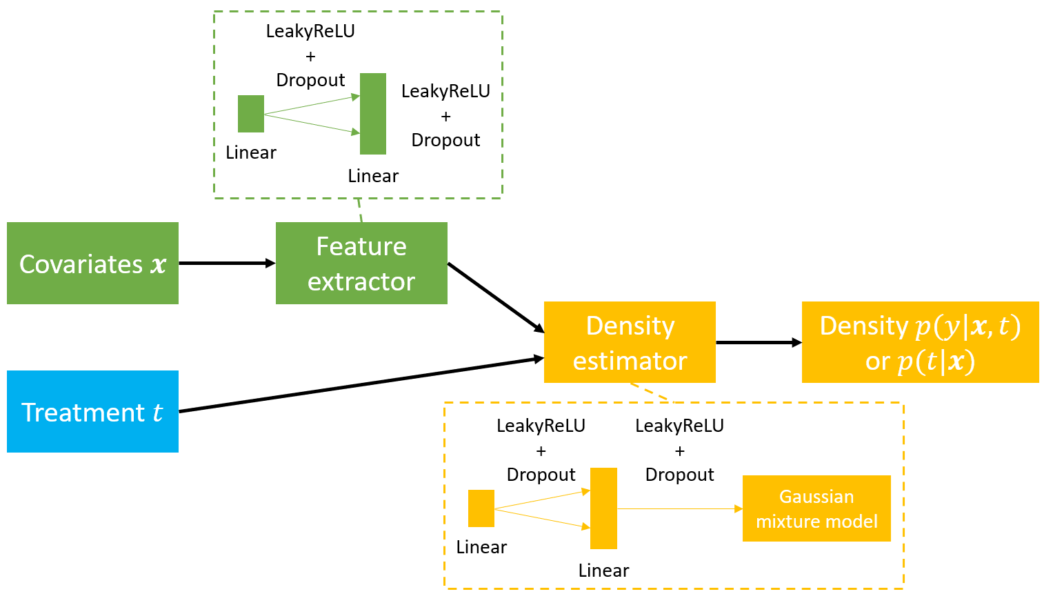
Figure 5: Gaussian Mixture Model Neural Network Architecture (inspired by [17])

Table 1: Neural Network Hyperparameters

	Hyperparameter	Value
Feature extractor	Linear 1 (hidden units)	Fine-tuned (8, 16, 32 or 64)
	Linear 2 (hidden units)	Fine-tuned (8, 16, 32 or 64)
	Leaky ReLU (negative slope)	0.04
	Dropout (probability)	0.04
Density estimator	Linear 1 (hidden units)	Fine-tuned (16, 32, 64 or 128)
	Linear 2 (hidden units)	Fine-tuned (16, 32, 64 or 128)
	Leaky ReLU (negative slope)	0.04
	Dropout (probability)	0.04
	Number of Gaussian components ($K$)	Fine-tuned (between 3 and 30)

Algorithm 2 Fine-Tuning Algorithm for a Gaussian Mixture Model Neural Network

Dataset $\mathcal{D}$, list of hyperparameters $(L_{1},\dots,L_{M})$ (search space), number of random splits $N$, neural network model $\mathcal{N}$, $\ell$ loss function

for $i\in[\![1,N]\!]$ do

     Divide $\mathcal{D}$ randomly into $\mathcal{D}^{\mathrm{train}}$ (80%), $\mathcal{D}^{\mathrm{valid}}$ (10%), $\mathcal{D}^{\mathrm{test}}$ (10%).

     for $c\in[\![1,M]\!]$ do

         Train $\mathcal{N}$ with hyperparameters $L_{c}$ on $\mathcal{D}_{i}^{\mathrm{train}}$ and use $\mathcal{D}_{i}^{\mathrm{valid}}$ for early stopping.

         Compute $l_{i,c}=\ell(\mathcal{D}_{i}^{\mathrm{test}})$.

     end for

end for

For all $c\in[\![1,M]\!]$, compute $l_{c}=\frac{1}{N}\sum_{i=1}^{N}l_{i,c}$.

Choose $L_{\hat{c}}$ with $\hat{c}=\operatorname*{argmin}_{c\in[\![1,M]\!]}l_{c}$.

B.2.1 Modeling of the GPS $\hat{f}(T=t|\mathbf{X}=\mathbf{x})$

In the same way as $\hat{f}(Y=y|\mathbf{X}=\mathbf{x},T=t)$, the GPS can be written as a mixture of $K^{\prime}$ Gaussian components

$$\hat{f}(T=t|\mathbf{X}=\mathbf{x})=\sum_{k=1}^{K^{\prime}}\tilde{\pi}_{k}(\mathbf{x})\mathcal{N}(t|\tilde{\mu}_{k}(\mathbf{x}),\tilde{\sigma}_{k}^{2}(\mathbf{x})),$$

where $\tilde{\pi}_{k}(\mathbf{x})$, $\tilde{\mu}_{k}(\mathbf{x})$ and $\tilde{\sigma}_{k}^{2}(\mathbf{x})$ are, respectively, the weight, mean and variance of the $k$^th component.

B.3 Conditional Quantile Estimation

To estimate the quantile function $Q(\upsilon;Y|\mathbf{X}=\mathbf{X}_{i},T=T_{i})$, we compute the conditional density $f(Y=y|\mathbf{X}=\mathbf{X}_{i},T=T_{i})$ and then search the root of the function $y\mapsto F(Y=y|\mathbf{X}=\mathbf{X}_{i},T=T_{i})-\upsilon$ thanks to the uniroot function from the stats library [26]. The cumulative distribution $F$ is recovered thanks to the cdf attribute of the estimated Gaussian mixture model. As the outcome $Y$ is centered and scaled, we search the root in the range $[-10,10]$.

B.4 Implementation Choices for the Method from [17]

We implement the algorithm from [17] in the R language, as it is only available for Python (see https://github.com/oatml/overcast). In particular, to estimate $f(Y=y|\mathbf{X}=\mathbf{x},T=t)$ and $\eta(t,\mathbf{x})$, we use the same model as for our method and the architecture from Figure 5. Moreover, as their method involves a Monte-Carlo integration (function $I(\cdot)$ from their paper), we sample 500 outcomes $Y_{i}$ from the estimated conditional density $f(Y=y|\mathbf{X}=\mathbf{x},T=t)$. To get the estimated lower and upper bounds for the APO (denoted $\underline{\hat{\mu}}(t;\Lambda,\theta)$ and $\hat{\bar{\mu}}(t;\Lambda,\theta)$, respectively, in [17]), we average the estimated bounds for the CAPO on all observed covariates, not only a subset as suggested in their article.

B.5 Details about the Simulated Dataset and Additional Results

B.5.1 Simulation Setup

The joint distribution $(\mathbf{X},\mathbf{U})$ follows a normal distribution $\mathcal{N}(\mathbf{0},\mathbf{\Sigma})$, where

$$\mathbf{\Sigma}=\begin{pmatrix}\mathbf{\Sigma_{X}}&\mathbf{\Sigma_{XU}}\\ \mathbf{\Sigma_{XU}}^{\top}&\mathbf{\Sigma_{U}}\end{pmatrix}.$$

$\mathbf{\Sigma_{X}}$ (resp., $\mathbf{\Sigma_{U}}$) is a tridiagonal matrix of size $p_{\mathbf{X}}\times p_{\mathbf{X}}$ (resp., $p_{\mathbf{U}}\times p_{\mathbf{U}}$), where the elements on the main diagonal are all equal to 1 and the elements on the subdiagonal and lower diagonal are all equal to $\rho_{\mathbf{X}}>0$ (resp., $\rho_{\mathbf{U}}>0$). $\mathbf{\Sigma_{XU}}$ is a $p_{\mathbf{X}}\times p_{\mathbf{U}}$ matrix with all coefficients equal to $\rho_{\mathbf{XU}}\geq 0$, where $\rho_{\mathbf{XU}}=\lambda\rho_{\mathbf{XU}}^{\mathrm{max}}$, with $0\leq\lambda<1$ and $\rho_{\mathbf{XU}}^{\mathrm{max}}=(1-\rho_{\mathbf{X}})/p_{\mathbf{U}}$, to ensure that $\mathbf{\Sigma}$ is a diagonal dominant matrix and is, thus, invertible.

The properties of the multivariate normal distribution allow to say that

$$\leavevmode\resizebox{234.15271pt}{}{$\mathbf{U}|\mathbf{X}=\mathbf{x}\sim\mathcal{N}\left(\mathbf{\Sigma_{XU}}^{\top}\mathbf{\Sigma_{X}}^{-1}\mathbf{x},\,\mathbf{\Sigma_{U}}-\mathbf{\Sigma_{XU}}^{\top}\mathbf{\Sigma_{X}}^{-1}\mathbf{\Sigma_{XU}}\right)$}.$$

We define $T$ conditionally on $\mathbf{X}=\mathbf{x},\mathbf{U}=\mathbf{u}$ as $T=\langle\beta_{\mathbf{X}},\mathbf{x}\rangle+\langle\beta_{\mathbf{U}},\mathbf{u}\rangle-0.5+\varepsilon_{T}$ where $\varepsilon_{T}\sim\mathcal{N}(0,\sigma_{\varepsilon_{T}}^{2})$, with $\sigma_{\varepsilon_{T}}>0$, $\beta_{\mathbf{X}}\in\mathbb{R}^{p_{\mathbf{X}}}$ and $\beta_{\mathbf{U}}\in\mathbb{R}^{p_{\mathbf{U}}}$. Moreover, the distribution of $T$ is given by $\mathcal{N}(\mu_{T},\sigma_{T}^{2})$, where

$$\mu_{T} =\phi_{X}(\mathbf{x})+\left\langle\beta_{\mathbf{U}},\,\mathbf{\Sigma_{XU}}^{\top}\mathbf{\Sigma_{X}}^{-1}\mathbf{x}\right\rangle\quad\text{and}$$

$$\sigma_{T}^{2} =\sigma_{\varepsilon_{T}}^{2}+\beta_{\mathbf{U}}^{\top}\bigl{(}\mathbf{\Sigma_{U}}-\mathbf{\Sigma_{XU}}^{\top}\mathbf{\Sigma_{X}}^{-1}\mathbf{\Sigma_{XU}}\bigr{)}\beta_{\mathbf{U}}.$$

Finally, for all $t\in\mathcal{T}$, we set the potential outcome to

$$Y(t)=t+\zeta\langle\mathbf{X},\gamma_{\mathbf{X}}\rangle\cdot e^{-t\langle\mathbf{X},\gamma_{\mathbf{X}}\rangle}-\langle\mathbf{U},\gamma_{\mathbf{U}}\rangle\langle\mathbf{X},\gamma_{\mathbf{X}}\rangle+\varepsilon_{Y}$$

where $\varepsilon_{Y}\sim\mathcal{N}(0,\sigma_{\varepsilon_{Y}}^{2})$, $\sigma_{\varepsilon_{Y}}>0$, $\zeta\in\mathbb{R}$, $\gamma_{\mathbf{X}}\in\mathbb{R}^{p_{\mathbf{X}}}$ and $\gamma_{\mathbf{U}}\in\mathbb{R}^{p_{\mathbf{U}}}$.

For all $\mathbf{x}\in\mathcal{X}$, the true CAPO is then

$$\theta(\tau,\mathbf{x})=\tau+\zeta\langle\mathbf{x},\gamma_{\mathbf{X}}\rangle e^{-\tau\langle\mathbf{x},\gamma_{\mathbf{X}}\rangle}-\left\langle\mathbf{\Sigma_{XU}}^{\top}\mathbf{\Sigma_{X}}^{-1}\mathbf{x},\gamma_{\mathbf{U}}\right\rangle\left\langle\mathbf{x},\gamma_{\mathbf{X}}\right\rangle,$$

and the true APO is given by

$$\theta(\tau)=\tau\Bigl{(}1-\zeta\cdot\gamma_{\mathbf{X}}^{\top}\mathbf{\Sigma_{X}}\gamma_{\mathbf{X}}\cdot e^{\frac{\tau^{2}}{2}\gamma_{\mathbf{X}}^{\top}\mathbf{\Sigma_{X}}\gamma_{\mathbf{X}}}\Bigr{)}-\gamma_{\mathbf{U}}^{\top}\mathbf{\Sigma_{XU}}^{\top}\gamma_{\mathbf{X}}.$$

During the simulation process, in order to avoid isolated data points, the observations that correspond to the 10% biggest hat values of the $(\mathbf{X},T,Y)$ design matrix are removed.

In our implementation, for reproducibility purpose, we set the random seeds to 1 (base R set.seed function and torch_manual_seed function from the torch library). Figure 6 is an example of a simulated sample with parameters from Table 2 and initial $n=1000$.

Figure 6: Example of a Simulated Sample (Treatment and Outcome) with Parameters from Table 2 and Initial $n=1000$. The Pink Curve Corresponds to the True Unknown APO Function $\theta(\tau)$.

B.5.2 Additional Sensitivity Analysis Results

Figure 7 is a sensitivity analysis performed on the data from Figure 6.

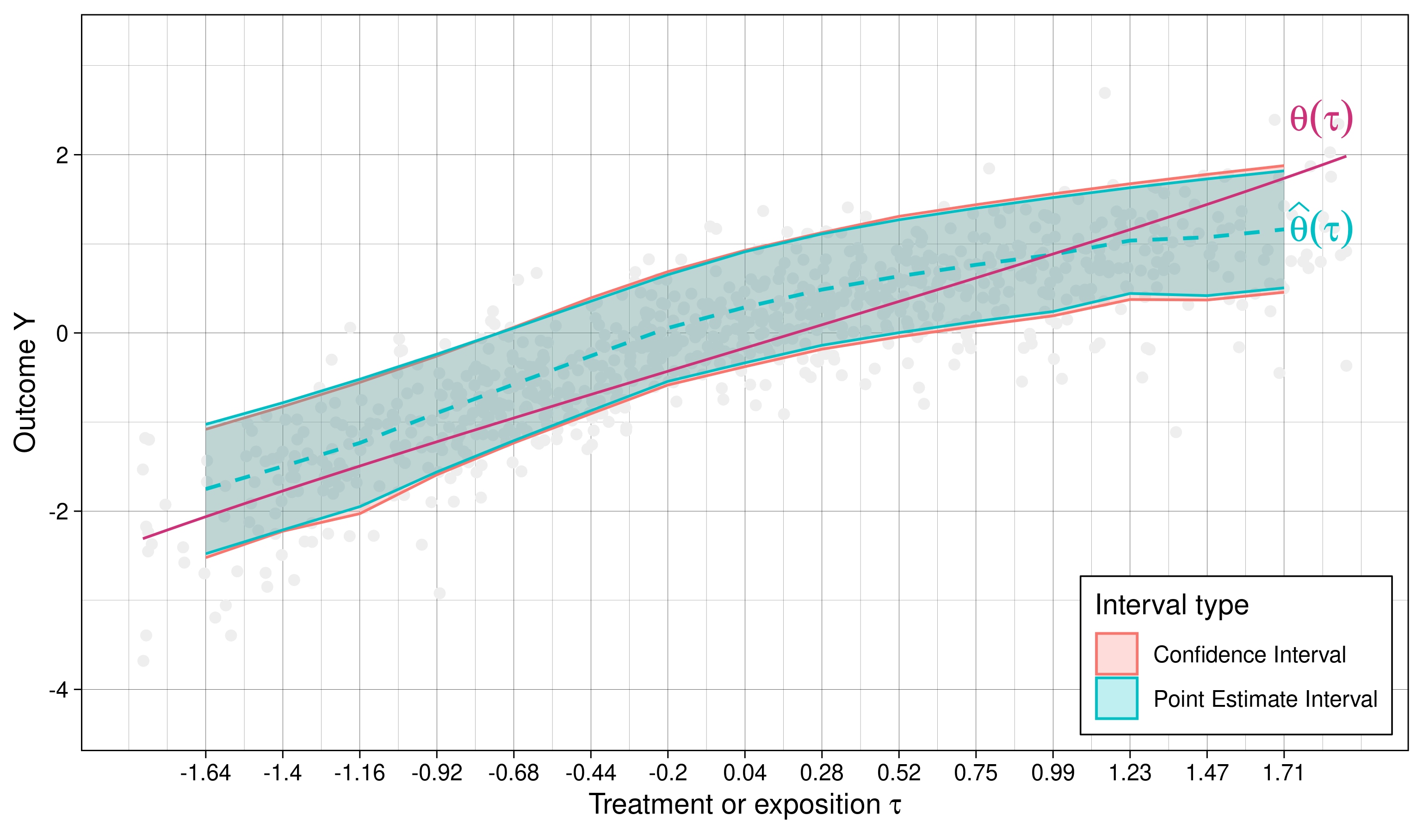
Figure 7: Sensitivity Analysis on the Simulated Dataset from Figure 6 for 15 Values of $\tau$. The Pink Line Corresponds to the True Unknown APO Function $\theta(\tau)$. The Blue Dotted Curve Corresponds to the Estimated APO Function $\hat{\theta}(\tau)$ Under Ignorability. The Gray Points Correspond to the Whole Generated Dataset. The Red Curves Correspond to the Estimated 95%-Level Confidence Intervals and the Blue Curves, to the Point Estimate Intervals.

Figures 1 and 2 in the main text are generated using the parameter values from Table 2.

Table 2: Parameter Values Used to Generate Figures 1 and 2

Parameter	Value	Parameter	Value	Parameter	Value
$p_{\mathbf{X}}$	5	$\lambda$	0.5	$\gamma_{\mathbf{U}}$	(0.4, 0.7, 0.7)
$p_{\mathbf{U}}$	3	$\beta_{\mathbf{X}}$	(0.3, 0.3, 0.3, 0.3, 0.3)	$\zeta$	-0.3
$\rho_{\mathbf{X}}$	0.3	$\beta_{\mathbf{U}}$	(0.2, 0.2, 0.2)	$\sigma_{\varepsilon_{T}}$	0.5
$\rho_{\mathbf{U}}$	0.3	$\gamma_{\mathbf{X}}$	(0.2, 0.2, 0.2, 0.2, 0.2)	$\sigma_{\varepsilon_{Y}}$	0.7

The doubly robust (DR) estimator from Proposition 3.3 is compared to the partially robust estimator and to the method from [17] in Figure 8. A higher variance in the estimation of the bounds with the DR method can be observed immediately. Moreover, the property of sharpness of the bounds tends to be valid for $\tau=-0.799$ and 0.0376 but not for other values. Finally, the coverage of the true APO is not good for extreme values of $\tau$. More investigations are needed to fully explain these results.

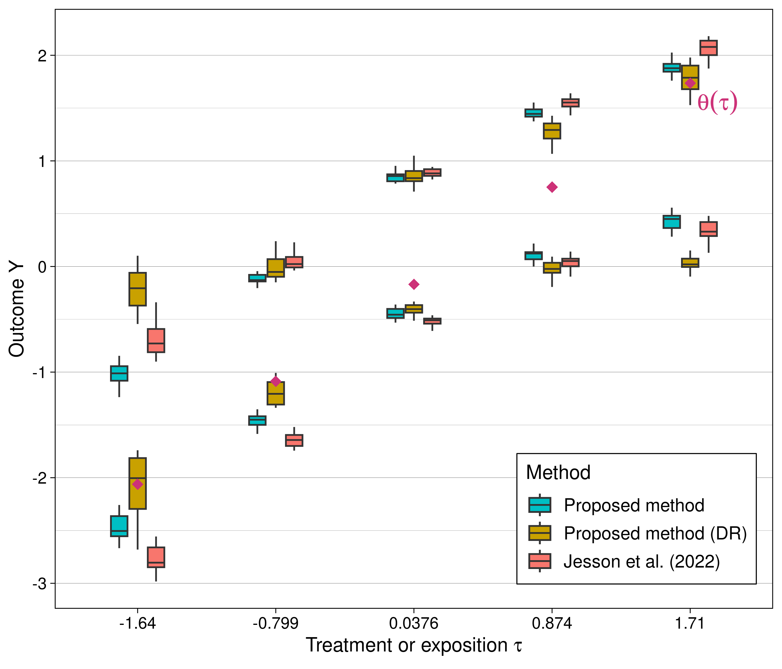
Figure 8: Boxplots of 95%-Level Confidence Intervals for 20 Monte-Carlo Samples. The Partially Robust Bounds Are in Blue While the Doubly Robust (DR) Ones Are in Yellow and the Ones from the Concurrent Method [17] Are in Red. The True APO is Represented by Pink Squares. The Data Are Generated Using the Setup from Table 2, with an Estimated $\Gamma$ of 5.21.

B.5.3 Computation Time Issue

In order to reduce execution time, it is possible to perform parallel computing. However, for practical reasons, it was not possible to use this technique because the tensor objects from the torch library do not allow parallelization. Figure 1 was therefore obtained with no parallel computing. Nevertheless, some parts in the code that did not involve torch tensors could be parallelized (essentially for the method from [17]). Thus, when possible, except for Figure 1, we used parallel computation on Amazon EC2 c6i.16xlarge instances.

B.5.4 Effect of the Parameters from the Data Generation Process on $\Gamma$

We perform an exploratory analysis of the influence of the parameters from the generation process of the dataset on the sensitivity parameter $\Gamma$. Figure 9 displays the influence of the correlation between $\mathbf{X}$ and $\mathbf{U}$, $\rho_{\mathbf{XU}}$, on the chosen $\Gamma$. As expected this sensitivity parameter decreases as the correlation increases, because already observed covariates would explain unobserved confounders. Then, in Figure 10, we vary the values of $\beta_{\mathbf{U}}$, which links the unobserved confounders to the treatment $T$. When $\mathbf{U}$ has no effect on the treatment, i.e. $\beta_{\mathbf{U}}$ is null, we expect $\Gamma$ to be equal to 1, which is equivalent to $\mathbf{X}$-ignorability. This is indeed what we observe in Figure 10, with $\Gamma$ values increasing as $\beta_{\mathbf{U}}$ becomes larger.

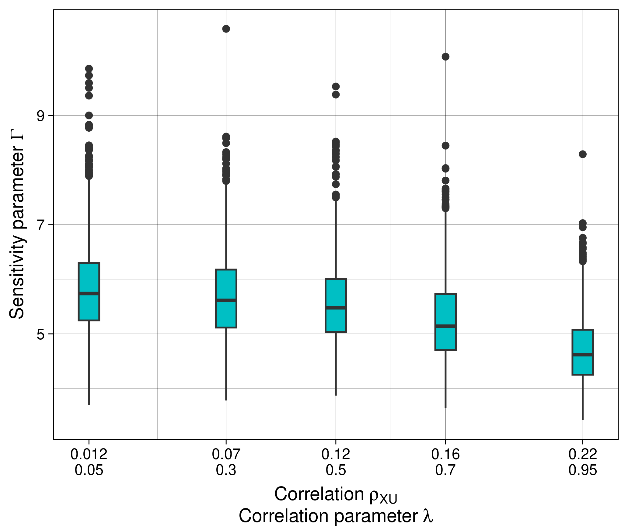
Figure 9: Boxplots of Estimated Sensitivity Parameter $\Gamma$ on 1000 Monte-Carlo Samples for 5 Values of Correlation $\rho_{\mathbf{XU}}$ (Setup from Table 2 except for $\rho_{\mathbf{XU}}$).

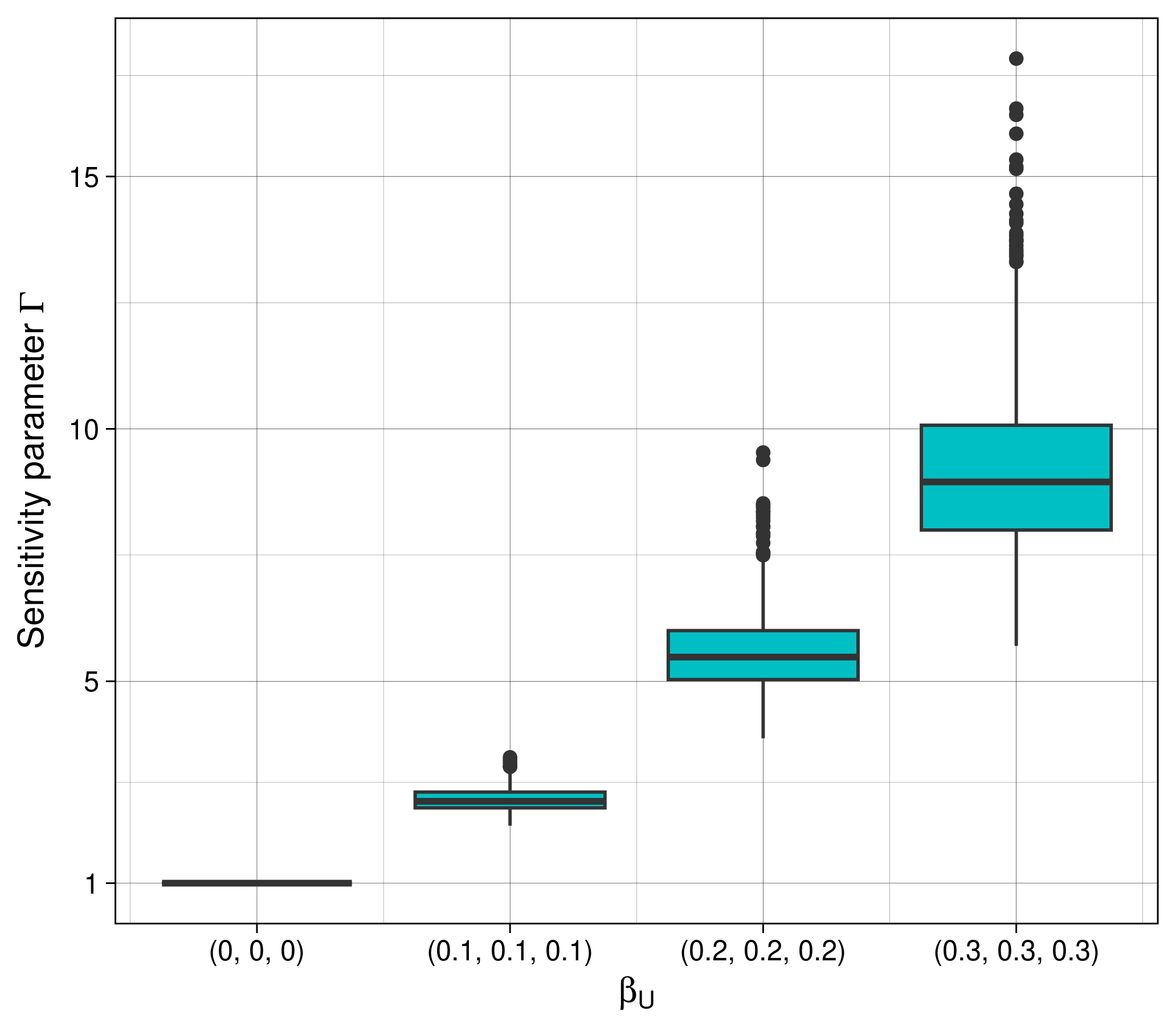
Figure 10: Boxplots of Estimated Sensitivity Parameter $\Gamma$ on 1000 Monte-Carlo Samples for 4 Values of $\beta_{\mathbf{U}}$ (Setup from Table 2 except for $\beta_{\mathbf{U}}$).

B.6 Details about the Real Dataset and Additional Results

The data are shared between three files: County_annual_PM25_CMR.csv, County_RAW_variables.csv and County_SES_index_quintile.csv.

The exposition $T$ is retrieved via the PM2.5 variable, and the observed outcome $Y$, via the CMR variable.

We keep 10 continuous variables that correspond to the observed confounders $\mathbf{X}$: healthfac_2005_1999, population_2000, SES_index_2010, civil_unemploy_2010, median_HH_inc_2010, femaleHH_ns_pct_2010, vacant_HHunit_2010, owner_occ_pct_2010, eduattain_HS_2010 and pctfam_pover_2010.

Only data from year 2010 are kept thanks to the Year variable. Then, population_2000 and median_HH_inc_2010 are log-normalized. Finally, CMR, PM2.5 and all covariates are centered and scaled. As in the simulated data, we remove 10% of the isolated data points that correspond to the 10% biggest hat values of the design matrix of $(\mathbf{X},T,Y)$.

Figure 11 shows the distribution of the outcome (CMR) as a function of the exposition (PM2.5) without the outliers, and before centering and scaling.

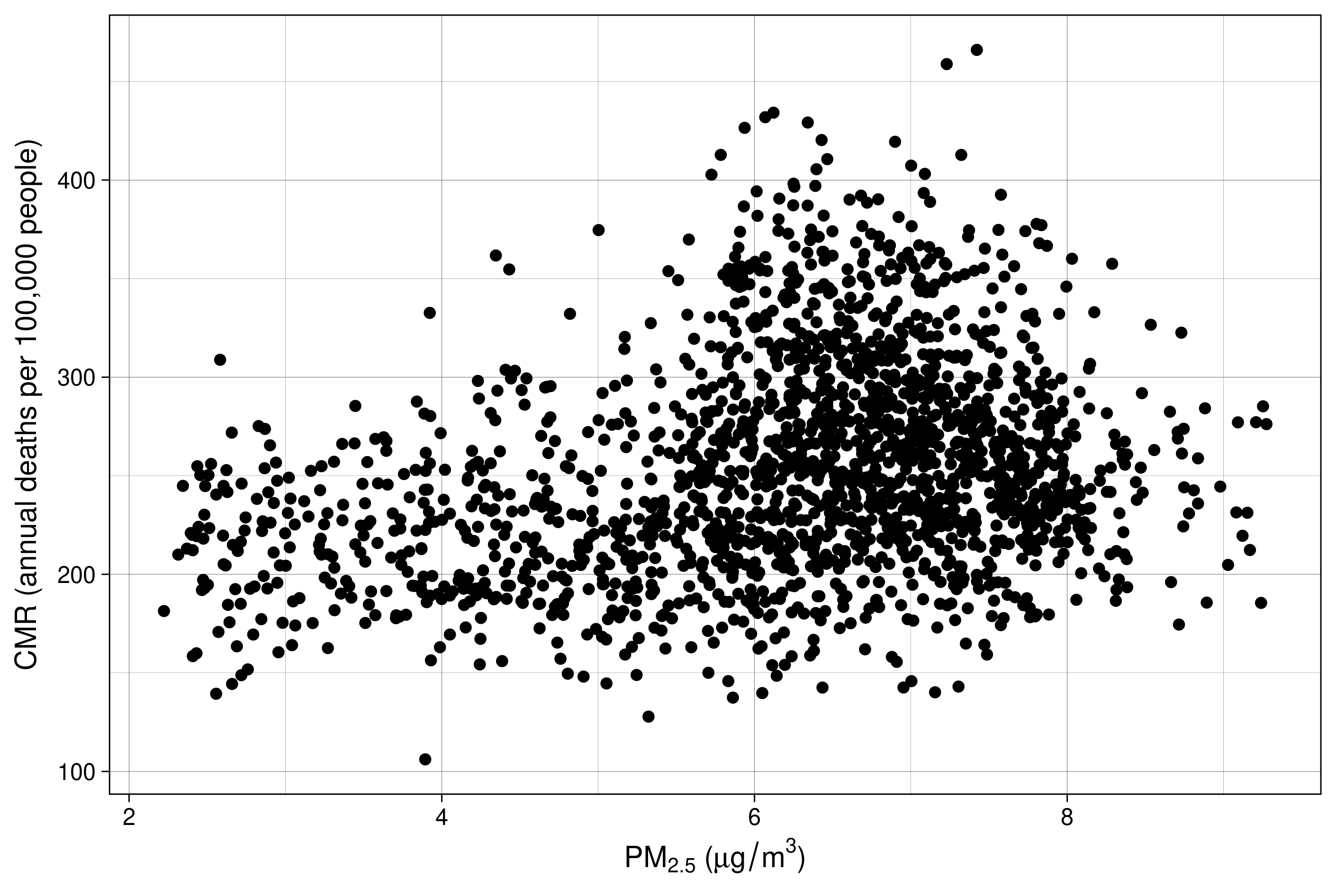
Figure 11: CMR as a Function of PM2.5.

Figure 12 is the same sensitivity analysis as in Figure 3, but with $\Gamma=50$ as well. However, high values of $\Gamma$ lead to extreme conditional quantiles, for which more suitable estimation methods than the one used in this paper should be used.

Figure 12: Sensitivity Analysis of the Real Dataset (95%-Level Confidence Intervals) with the Proposed Method and the One from [17] for 6 Values of $\Gamma$ and 15 Values of Exposition $\tau$ (PM2.5). The Red Dotted Line Corresponds to the Average CMR (255 Annual Deaths per 100,000 People). The Gray Points Are the Real Dataset With 82 Observations Removed to Improve Readability.

B.7 Libraries and Licenses

Libraries from Table 3 are used in the proposed R implementation.

Table 3: Libraries and Corresponding Licenses

Library	Authors	Version	License
foreach	[24]	1.5.2	Apache License (== 2.0)
ggplot2	[36]	3.4.4	MIT
latex2exp	[23]	0.9.6	MIT
tictoc	[16]	1.2.1	Apache License (== 2.0)
torch	[9]	0.12.0	MIT

References

• [1] Ruben G Ascoli โ€œLimitations Of Richardson Extrapolation For Kernel Density Estimationโ€ In arXiv preprint arXiv:1812.08619, 2018
• [2] Susan Athey, Julie Tibshirani and Stefan Wager โ€œGeneralized random forestsโ€ In The Annals of Statistics 47.2 Institute of Mathematical Statistics, 2019, pp. 1148โ€“1178 DOI: 10.1214/18-AOS1709
• [3] Taha Bahadori, Eric Tchetgen Tchetgen and David Heckerman โ€œEnd-to-end balancing for causal continuous treatment-effect estimationโ€ In International Conference on Machine Learning, 2022, pp. 1313โ€“1326 PMLR
• [4] Christopher M. Bishop โ€œMixture density networksโ€ Aston University, 1994
• [5] Kyle Colangelo and Ying-Ying Lee โ€œDouble Debiased Machine Learning Nonparametric Inference with Continuous Treatmentsโ€, 2023 arXiv: https://arxiv.org/abs/2004.03036
• [6] Peng Ding et al. โ€œSensitivity Analysis for Unmeasured Confounding in Medical Product Development and Evaluation Using Real World Evidenceโ€ In arXiv preprint arXiv:2307.07442, 2023
• [7] Jacob Dorn and Kevin Guo โ€œSharp sensitivity analysis for inverse propensity weighting via quantile balancingโ€ In Journal of the American Statistical Association Taylor & Francis, 2022, pp. 1โ€“13
• [8] Jacob Dorn, Kevin Guo and Nathan Kallus โ€œDoubly-valid/doubly-sharp sensitivity analysis for causal inference with unmeasured confoundingโ€ In Journal of the American Statistical Association Taylor & Francis, 2024, pp. 1โ€“12
• [9] Daniel Falbel and Javier Luraschi โ€œtorch: Tensors and Neural Networks with โ€™GPUโ€™ Accelerationโ€ R package version 0.12.0, https://github.com/mlverse/torch, 2023 URL: https://torch.mlverse.org/docs
• [10] Julian J. Faraway and Myoungshic Jhun โ€œBootstrap Choice of Bandwidth for Density Estimationโ€ In Journal of the American Statistical Association 85.412 [American Statistical Association, Taylor & Francis, Ltd.], 1990, pp. 1119โ€“1122 URL: http://www.jstor.org/stable/2289609
• [11] Alexander Goldenshluger and Oleg Lepski โ€œBandwidth selection in kernel density estimation: Oracle inequalities and adaptive minimax optimalityโ€ In The Annals of Statistics 39.3 Institute of Mathematical Statistics, 2011, pp. 1608โ€“1632 DOI: 10.1214/11-AOS883
• [12] Martin Herdegen and Cosimo Munari โ€œAn elementary proof of the dual representation of Expected Shortfallโ€ In Mathematics and Financial Economics 17.4 Springer, 2023, pp. 655โ€“662
• [13] Jennifer L Hill โ€œBayesian nonparametric modeling for causal inferenceโ€ In Journal of Computational and Graphical Statistics 20.1 Taylor & Francis, 2011, pp. 217โ€“240
• [14] Keisuke Hirano and Guido W Imbens โ€œThe propensity score with continuous treatmentsโ€ In Applied Bayesian modeling and causal inference from incomplete-data perspectives 226164, 2004, pp. 73โ€“84
• [15] Kosuke Imai and David A Van Dyk โ€œCausal inference with general treatment regimes: Generalizing the propensity scoreโ€ In Journal of the American Statistical Association 99.467 Taylor & Francis, 2004, pp. 854โ€“866
• [16] Sergei Izrailev โ€œtictoc: Functions for Timing R Scripts, as Well as Implementations of โ€Stackโ€ and โ€StackListโ€ Structuresโ€ R package version 1.2.1, 2024 URL: https://CRAN.R-project.org/package=tictoc
• [17] Andrew Jesson et al. โ€œScalable sensitivity and uncertainty analyses for causal-effect estimates of continuous-valued interventionsโ€ In Advances in Neural Information Processing Systems 35, 2022, pp. 13892โ€“13907
• [18] Ying Jin, Zhimei Ren and Emmanuel J Candรจs โ€œSensitivity analysis of individual treatment effects: A robust conformal inference approachโ€ In Proceedings of the National Academy of Sciences 120.6 National Acad Sciences, 2023, pp. e2214889120
• [19] Nathan Kallus and Angela Zhou โ€œConfounding-robust policy improvementโ€ In Advances in neural information processing systems 31, 2018
• [20] Nathan Kallus and Angela Zhou โ€œPolicy evaluation and optimization with continuous treatmentsโ€ In International conference on artificial intelligence and statistics, 2018, pp. 1243โ€“1251 PMLR
• [21] Amirreza Kazemi and Martin Ester โ€œAdversarially Balanced Representation for Continuous Treatment Effect Estimationโ€ In Proceedings of the AAAI Conference on Artificial Intelligence 38.12, 2024, pp. 13085โ€“13093
• [22] Edward H Kennedy, Zongming Ma, Matthew D McHugh and Dylan S Small โ€œNon-parametric methods for doubly robust estimation of continuous treatment effectsโ€ In Journal of the Royal Statistical Society Series B: Statistical Methodology 79.4 Oxford University Press, 2017, pp. 1229โ€“1245
• [23] Stefano Meschiari โ€œlatex2exp: Use LaTeX Expressions in Plotsโ€ R package version 0.9.6, 2022 URL: https://CRAN.R-project.org/package=latex2exp
• [24] Microsoft and Steve Weston โ€œforeach: Provides Foreach Looping Constructโ€ R package version 1.5.2, 2022 URL: https://CRAN.R-project.org/package=foreach
• [25] Jerzy Neyman โ€œOn the application of probability theory to agricultural experiments. Essay on principlesโ€ In Ann. Agricultural Sciences, 1923, pp. 1โ€“51
• [26] R Core Team โ€œR: A Language and Environment for Statistical Computingโ€, 2023 R Foundation for Statistical Computing URL: https://www.R-project.org/
• [27] R Tyrrell Rockafellar and Stanislav Uryasev โ€œOptimization of conditional value-at-riskโ€ In Journal of risk 2 Citeseer, 2000, pp. 21โ€“42
• [28] P.R. Rosenbaum โ€œObservational Studiesโ€, Springer Series in Statistics Springer, 2002 URL: https://books.google.fr/books?id=K0OglGXtpGMC
• [29] Paul R Rosenbaum and Donald B Rubin โ€œThe central role of the propensity score in observational studies for causal effectsโ€ In Biometrika 70.1 Oxford University Press, 1983, pp. 41โ€“55
• [30] Jonas Rothfuss, Fabio Ferreira, Simon Walther and Maxim Ulrich โ€œConditional density estimation with neural networks: Best practices and benchmarksโ€ In arXiv preprint arXiv:1903.00954, 2019
• [31] Donald B Rubin โ€œEstimating causal effects of treatments in randomized and nonrandomized studies.โ€ In Journal of educational Psychology 66.5 American Psychological Association, 1974, pp. 688
• [32] BW Silverman and GA Young โ€œThe bootstrap: to smooth or not to smooth?โ€ In Biometrika 74.3 Oxford University Press, 1987, pp. 469โ€“479
• [33] Masashi Sugiyama et al. โ€œConditional density estimation via least-squares density ratio estimationโ€ In Proceedings of the Thirteenth International Conference on Artificial Intelligence and Statistics, 2010, pp. 781โ€“788 JMLR WorkshopConference Proceedings
• [34] Zhiqiang Tan โ€œA distributional approach for causal inference using propensity scoresโ€ In Journal of the American Statistical Association 101.476 Taylor & Francis, 2006, pp. 1619โ€“1637
• [35] Alexandre B Tsybakov โ€œNonparametric estimatorsโ€ In Introduction to Nonparametric Estimation Springer, 2009, pp. 1โ€“76
• [36] Hadley Wickham โ€œggplot2: Elegant Graphics for Data Analysisโ€ Springer-Verlag New York, 2016 URL: https://ggplot2.tidyverse.org
• [37] Lauren H Wyatt et al. โ€œAnnual PM2. 5 and cardiovascular mortality rate data: Trends modified by county socioeconomic status in 2,132 US countiesโ€ In Data in brief 30 Elsevier, 2020, pp. 105318
• [38] Steve Yadlowsky et al. โ€œBounds on the conditional and average treatment effect with unobserved confounding factorsโ€ In The Annals of Statistics 50.5 Institute of Mathematical Statistics, 2022, pp. 2587โ€“2615
• [39] Qingyuan Zhao, Dylan S Small and Bhaswar B Bhattacharya โ€œSensitivity analysis for inverse probability weighting estimators via the percentile bootstrapโ€ In Journal of the Royal Statistical Society Series B: Statistical Methodology 81.4 Oxford University Press, 2019, pp. 735โ€“761