A bifurcation phenomenon for the critical Laplace and -Laplace equation in the ball
Francesca Dalbono
Matteo Franca
Andrea Sfecci
Dipartimento di Matematica e Informatica, Università degli Studi di Palermo,
Via Archirafi 34, 90123 Palermo - Italy. email: francesca.dalbono@unipa.it
Dipartimento di Matematica,
Università degli Studi di Bologna, Piazza di porta san Donato 5 - 40126, Bologna -
Italy. email: matteo.franca4@unibo.it Dipartimento di Matematica e Geoscienze,
Università degli Studi di Trieste, Via Valerio 12/1, 34127, Trieste -
Italy. email: asfecci@units.it.
(Received: date / Accepted: date)
Abstract
In this paper we show that the number of radial positive solutions of the following critical problem
where , and ,
undergoes a bifurcation phenomenon.
Namely, the problem admits one solution for any if is steep enough at , while it admits no solutions
for small and two solutions for large if is too flat at .
The existence of the second solution is new, even in the classical Laplace case.
The proofs use Fowler transformation and dynamical systems tools.
In this paper we focus on positive radial solutions for the generalized scalar curvature equation
(1)
where denotes the -Laplace operator,
,
,
, and is the Sobolev critical exponent
(2)
The function is assumed to be , for simplicity.
We are interested in crossing solutions, which means solutions of the problem
(3)
In particular, we will show that the existence of radial solutions of (3) depends on the behavior of
in a neighborhood of zero, and on the length of the radius .
Since we exclusively concentrate our study on radial solutions, we can reduce equation (1) to
the following singular ordinary differential equation
(4)
where “ ” denotes the differentiation with respect to , and, with a slight
abuse of notation, .
We say that a solution of (4) is regular if and only if for a suitable : in this case it will be denoted by .
It is well known that exists and it is unique for any , cf. e.g. [25, 26, 33, 34].
Note that .
As an alternative, from a standard scaling argument, we can find a counterpart for the eigenvalue equation where we fix for definiteness and we multiply the potential by a parameter , i.e.
(5)
Indeed, if we set
(6)
and , then solves equation (4) if and only if solves
and if and only if , where .
Hence, the number of solutions of (3) as varies coincides with
the number of solutions of (5) as varies.
The scalar curvature equation (1) has been extensively studied in the literature due to its significance in a broad variety of applications, such as
Riemannian geometry, astrophysics, quantum mechanic, chemistry, theory of non-Newtonian fluids and elasticity (cf. [21] for more detailed references on application of -Laplace equations and e.g. [7, 8]
for application to Riemannian geometry in the case).
In many phenomena, positivity of solutions has a physical relevance.
Non-linear eigenvalue problems similar to (5) are nowadays a classical topic, see e.g. [5] and the more recent [6, 15, 16, 28, 40]
where the reaction term is replaced by a sum of a linear and a term either critical or supercritical with respect to the Sobolev exponent. We address the interested reader to the introduction of [5, 15, 16] for a discussion of several possible diagrams appearing as different reaction terms are considered.
A key role in our analysis is played by the following hypothesis
There are some constants such that
The existence and the multiplicity of the solutions of (3) and (5)
depend crucially on , which, in literature, is often referred to as the order of flatness of the function at .
Problem (3) subject to condition has been already investigated in the early 1990s
by Bianchi-Egnell in [3] and by Lin-Lin in [39], who determined the existence of the critical value
in the Laplacian setting . In fact, Bianchi-Egnell and Lin-Lin have been able to prove the following result.
Theorem A [39].Assume that satisfies and consider in (3).
If , then problem (3) admits a radial solution for every .
(
If , then there exists a sufficiently small constant such that problem (3)
does not admit any radial solution when ;
)
If , then there exists a sufficiently large constant such that problem (3) admits a radial solution
for every .
In fact Bianchi and Egnell in [3] focused on the case.
In particular, following a shooting approach based on ordinary differential equations, they constructed and glued together two regular solutions of (4), one shooting from the zero initial condition and the other shooting from infinity.
The restriction has often been adopted in the Laplacian literature to ensure the existence of a solution to problem (3).
For instance, it appears in [37, Theorem 0.19], where the scalar curvature is required to be strictly decreasing in a left neighbourhood of .
The upper constraint can be also found in the recent work [38], dealing with the -Nirenberg problem on the standard sphere
for .
Among the very few examples of existence results for the Laplacian scalar curvature problem
in the absence of upper bound conditions on ,
we refer to the very recent papers [10, 43], where hypothesis is combined with
a (not so easily verifiable) topological global index formula on the critical points of .
Note that in the -Laplace context, the condition generalizes to , cf. [22].
We emphasize that Theorem A, besides its intrinsic interest, has been a key starting point in proving
the existence of Ground States with fast decay, i.e. solutions positive for any and decaying as
at infinity.
In fact, it can be shown that if is increasing close to and decreasing close to
we might expect to find Ground States with fast decay: in the 90s there was a flourishing of papers giving sufficient conditions for existence and non-existence
of these solutions.
A possible strategy is indeed to combine Theorem A, or similar results, with the use of Kelvin inversion,
which transfers the information on regular solutions to fast decay solutions,
see e.g. [3, 12].
Roughly speaking, one can expect that if is steep enough at (i.e. ) and at infinity
with and , , then
there is a Ground State with fast decay, while if these conditions are violated, one can construct a counterexample to Theorem A, see [3, Theorem 0.3]. For a generalization to the -Laplace setting, we also refer to [22], which
follows a different strategy since Kelvin inversion is not available in that context.
We think it is worthwhile to point out that if in , then the problem becomes easier: roughly speaking,
its solutions behave as the solutions of the , -subcritical case,
i.e. (3) admits a radial solution for any (or, equivalently, (5) admits
a radial solution for any ), for any . Again, combining this result with Kelvin inversion one might obtain
the existence of Ground States with fast decay. This idea was extensively used in the 90s in many papers
to handle the Laplacian problem, starting, probably, from [35],
[9], [44],
and then it was developed and adapted to related problems, such as existence of Ground States with fast decay with a prescribed number of sign changes, see e.g. [45] and [33], dealing with the Laplacian and -Laplacian setting, respectively.
The aim of this paper is to improve Theorem A in 3 main directions.
Firstly, we extend the results to the -Laplace context, proving the existence of the generalized flatness order’s threshold
which coincides with
of Theorem A for .
As far as we are aware, these are the first results in this direction,
although
we have to require
the probably technical condition
. The possibility to remove this restriction will be the object of further investigations.
Secondly, we are able to remove the condition (i.e. in the -Laplace context), by requiring
that is increasing for any .
Thirdly, and probably more importantly, we are able to prove the existence of a second solution when
(i.e. in the -Laplace context), thus completing the bifurcation diagram even in the case.
Let us state our assumptions and the main results of the paper.
The function is increasing for any , strictly in some interval.
The function is uniformly continuous in and there are such that
for any .
Note that if is bounded in
then is uniformly continuous in .
Theorem 1.
Assume that satisfies .
If , then problem (3) admits a radial solution for every .
If , then there exists such that problem (3)
does not admit any radial solution when .
In fact, Theorem 2 holds also if we drop the global assumption ,
but we strengthen the requirement on by
introducing the upper bound on the order of flatness at zero, in the spirit of Theorem A.
Unfortunately, we need to ask for some further very weak technical conditions on for large.
Theorem 3.
Assume that satisfies with
.
Assume further that either holds or there is such that
when , then we get the same conclusion as in Theorem 2.
Using the change of variable (6), we can
rewrite Theorems 1, 2, and 3 as follows.
Corollary 4.
Assume that satisfies .
If , then problem (5) admits a radial solution for every .
If , then there exists such that problem (5)
does not admit any radial solution when .
Again, according to Theorem 3, we can drop the global condition and get the same result by restricting the interval in which varies
and by imposing some further weak asymptotic conditions on for large.
Corollary 6.
Assume that satisfies with ; assume further that either holds or there is such that
for any .
Then, we get the same conclusions as in Corollary 5.
In fact via Theorem 3 and Corollary 6
we are also able to extend Theorem A to the case where , which was not covered by [3, 39], with the addition of a very weak technical condition
which, roughly speaking, is satisfied unless is subject to wild oscillations for large, or converges to for large.
Moreover, our methods are considerably different from those of Lin-Lin in [39].
Our proofs are based on the Fowler transformation, which discloses the geometrical aspect of our problem by converting the singular ordinary differential equation (4)
into an equivalent dynamical system, cf. (11), following the way paved by [32, 31, 30] and later on by [1, 2, 23].
Then, we develop a detailed phase plane analysis, involving invariant manifold theory for non-autonomous systems, energy estimates, comparisons of the
non-autonomous planar system with suitable autonomous ones and a Grönwall’s argument.
1.1 On the proofs of the theorems
We briefly sketch the plan of our proof.
Let
(7)
and denote by the first zero of when :
our argument relies on a study of the properties of the function .
Using some classical results (see [14, 36] for the Laplacian
case, and [26, 34] for -Laplacian extensions),
we know that under assumption .
Then, using a standard transversality argument,
it is straightforwardly proved that is continuous, see Proposition 22 below.
Then, it is not difficult to show, see, e.g. [33, Proposition 2.4] that
(8)
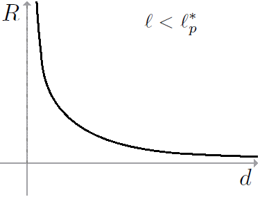
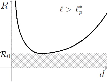
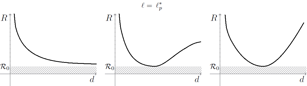
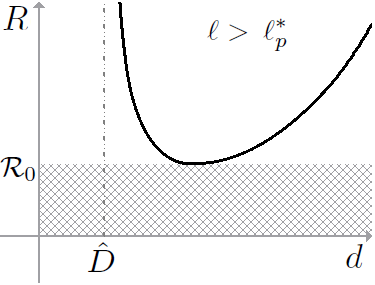
Figure 1: A sketch of the graph of the function , when and are assumed. In the critical case , we have three possible alternatives.
The focus and the original part of our study consists in analyzing the asymptotic behaviour of the solutions with large initial data ,
which is determined by the parameter in . In particular, we have the following
bifurcation phenomenon, when is assumed
(9)
see Propositions 37 and 43 below.
This asymptotic analysis will allow us to draw the diagrams in Figure 1.
Since the number of solutions of
problem (3) is the number of points of the preimage , the proof of Theorem 2 is immediately given.
Actually, using a truncation argument, see Remark 25, we are
able to get the first estimate in (9), also when assumption is dropped,
cf. Proposition 37. Hence, the proof of Theorem 1 in the subcritical case follows.
In fact, in the case, a part of (9)
has been already shown in [39, Theorem 1.6], see also [7, Remark 4.1]:
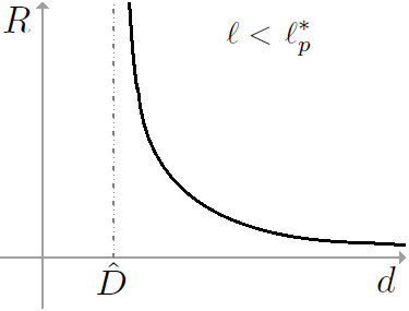
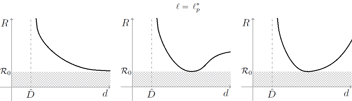
Figure 2: A sketch of the graph of the function , in the setting of Theorem 3. In the critical case , we have three possible alternatives.
Finally, we adapt our analysis to the context where the global requirement is replaced by the local requirement ,
and we reprove the existence of the second solution in the supercritical case. As shown in Lemma 45 below, the restriction , and the technical
requirement that either holds or there is such that when
are needed just
in order to ensure that there is such that , with as in (7).
Then, using classical arguments, we see that if , then
and, adapting the computation performed when holds, we prove that
satisfies (9) if ,
see Propositions 44 and 46 below.
As a consequence, we are able to draw the diagrams for in Figure 2,
from which Theorem 3 follows.
Notice that if , then is a Ground State, that is a solution of (4), positive for any .
The paper is organized as follows.
In §2 we introduce the Fowler transformation, i.e.
the change of variables (2) which turns (4) into the planar, non-autonomous dynamical system (11); then we recall some basic tools
in this context. In particular, we review some aspects of invariant manifold theory for non-autonomous systems,
and we introduce the unstable leaves of (11) which correspond to regular solutions
of (4).
In §3 we establish some standard properties of the function , such as continuity and
asymptotic properties close to and to , when is a Ground State.
The core of our argument is in §4, where we prove the asymptotic properties of as tends to infinity:
in §4.1 we focus on the subcritical case , and in §4.2 we consider the critical and supercritical setting
. In §5 we briefly conclude the proofs of the main results of the paper.
2 Fowler transformation,
basic notation and preliminaries
Let us introduce a change of variables known as Fowler transformation,
which allows to transform (4) into a two-dimensional dynamical system.
We define
(10)
This change of variable is known from the ’30s, see [17], and it has been generalized
to the -Laplacian case by Bidaut-Véron [4] and some years later (independently) by Franca, see e.g. [18, 19, 20, 22, 23].
According to (2), we can rewrite (4) as the following dynamical system:
(11)
where , as in (2),
and “” denotes the differentiation with respect to .
If we evaluate along a solution of (11), we obtain the associated Pohozaev type energy , whose derivative
with respect to satisfies
(14)
We also need to consider the autonomous system obtained by freezing the -dependence
of . In particular,
fixed ,
we consider the frozen autonomous system:
(15)
where is assumed to have finite limit, whenever .
If we differentiate the energy of system (15) along a solution
of the dynamical system (11), we get
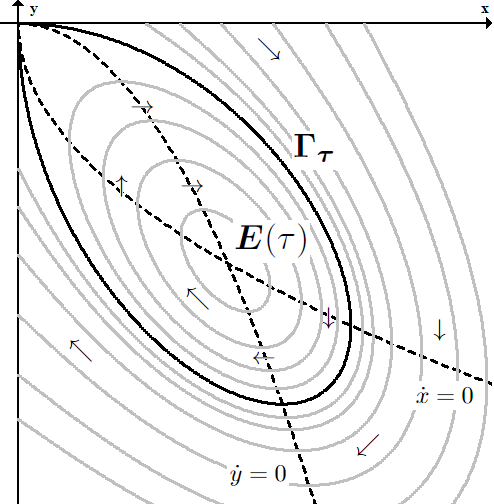
System (15) exhibits an equilibrium point in , of coordinates
(18)
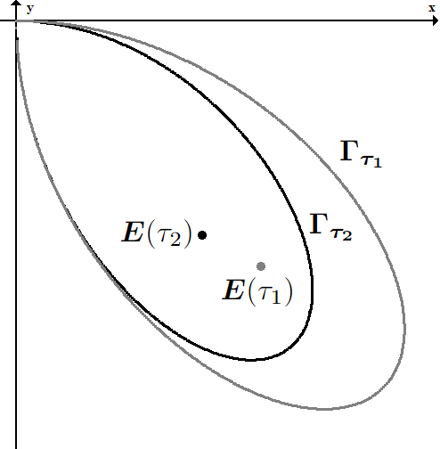
It is also well known (see, among others, [22]) that, for any fixed , system (15) admits a homoclinic orbit
(see Figure 3)
(19)
recalling that the case requires a boundedness restriction on .
Taking into account that the flows of (11) and (15) are ruled by their linear part near the origin,
we easily deduce that the origin is a
saddle-type critical point for (11) and (15).
Finally, notice that
is a centre and it lies in the interior of the region enclosed by .
According to [23, 27], we also know the exact expression of the homoclinic trajectories of (15). In particular, the one corresponding to the regular Ground State such that satisfies
(20)
where is a computable constant, see [27].
Moreover, fixed there exists a constant such that
(21)
where .
Let us now list some immediate consequences of assumption .
Remark 8.
Assume , then the homoclinic orbit belongs to the region enclosed by , cf. Figure 3.
Figure 3: On the left, the energy levels of at fixed time , with the homoclinic orbit . On the right, the position of the set with respect to the set in the case .
Lemma 9.
Assume .
If is a regular solution, then the corresponding trajectory of system (11)
satisfies
and
(the equality occurs only when holds),
where is the first zero of .
Moreover,
(the first equality occurs only when holds).
Proof.
The result immediately follows from , (14), and (13).
∎
As an immediate consequence we have the following.
Lemma 10.
Assume and fix . Then, for every , the trajectory of system (11)
either lies in the exterior of the region enclosed by , or it lies on if .
The next part of the section is devoted to explore the dynamical system (11) through an invariant manifold approach.
From [23, 29, 31], and [11, §13.4], we know that the existence of the unstable manifold is ensured by the following condition:
The function is bounded and uniformly continuous in and is finite.
Notice that is always satisfied when holds.
Correspondingly, the existence of the stable manifold is guaranteed by .
The unstable manifold will play a key role in this paper, since we will see via Remark 17
that regular solutions correspond to trajectories of (11) converging to the origin as ,
i.e. leaving from the unstable manifold.
Let
denote the open ball of radius , centered at the origin.
Following [31, Theorem 2.1], which is in fact a rewording of [29, Theorem 2.25], and its reformulation in[24, Appendix],
we find the next result.
Theorem 11.
Assume , then there is such that for any the set
is a embedded manifold tangent to the -axis at the origin if , and to the line if .
Further, let
be a segment
transversal to , then is a singleton,
and
is uniformly continuous in .
Assume , then there is such that for any the set
is a embedded manifold tangent to the -axis at the origin if and to the line if .
Further, let be a segment
transversal to , then is a singleton, and
is uniformly continuous in .
This result may also be obtained by using the simpler approach developed in [11, §13.4], with the exception of
the part concerning
the uniform continuity of and .
Actually, [31, Theorem 2.1] ensures that and are
if is .
We notice that
is split by the origin in two connected components.
Since we are just interested in positive solutions, we denote by and the components
lying respectively in and . Similarly,
is split by the origin in two connected components, say and ,
lying in and , respectively.
Following again either [29, Theorem 2.25]
or [11, §13.4] and in particular Theorem 4.5, we deduce some crucial properties concerning the uniform exponential asymptotic behaviour of the trajectories intersecting the manifolds and .
Theorem 12.
Assume and , then the sets
are embedded manifold for any . Furthermore,
if and , then
the limits
are positive and finite. Further, there is such that
Using the flow of (11), with a standard argument, we pass from the local manifolds
and , defined for , to the global manifolds and defined
for any .
In fact, rephrasing [24, Appendix],
we set
(22)
We observe that and , the unstable and stable leaves respectively, are immersed manifolds which can be characterized as follows
(23)
By construction, if , then for any .
From Theorem 11
and the smooth dependence of the flow of (11) on initial data,
we get the smoothness property of the unstable and stable manifold.
Remark 13.
Assume , then depends continuously on . Namely,
let be a segment which intersects transversely in a point , then
there is a neighborhood of such that
intersects in a point for any , and is continuous. Actually, it has the same
regularity as (11), so it is if (11) is in .
Analogously if holds, then depends continuously on , and smoothly if (11) is smooth in .
Let us denote by the unstable manifold , defined in (19).
According to [1] and [24, §2.2], the smoothness property of observed in Remark 13 can be extended to .
Remark 14.
Assume ,
then
depends smoothly on .
In particular, let be a segment transversal to and let be the intersection point between and ;
follow from the origin towards ,
then it intersects transversely in a point, say , for any ,
for a suitable sufficiently large
; furthermore, the function is and
.
We stress that is uniquely defined as the first
intersection between and , although it might not be the unique intersection,
especially if is too large.
Let be a segment transversal to , take and
denote by the compact and connected branch of between the origin and
.
Analogously, denote by the compact connected branch of
between the origin and .
Lemma 15.
Assume . Let and be as in Remark 14, then there is such that
(24)
Proof.
Let be the fixed constant defined in Theorem 11.
If is close enough to the origin so that , then
by construction
for every , see (22), and (24) follows straightforwardly from Theorem 12.
Now, let be a generic segment transversal to satisfying
, and let be such that
Fix a point belonging to , then
there is
such that
. By construction,
for any
since
.
Using Remark 14 combined with the compactness of , continuous dependence on initial data and parameters of the flow of (11),
and possibly choosing a larger ,
we can assume that
is such that
(25)
whenever and ; notice that does not depend on and , but depends on .
The existence of as in (25) is trivial for any , so
(25) holds for any .
Thus, Theorem 12 ensures the existence of such that
To prove (24) for ,
it is enough to recall that is compact, is fixed and the flow of (11) is continuous;
then the lemma follows by choosing some
.
∎
The following lemma better describes the behaviour of the solutions departing
from a point , as . Roughly speaking, we can say that such trajectories mime the autonomous dynamical system (15) frozen at .
If is unbounded,
then we easily get a contradiction with (27).
Thus, we can assume that there is such that
.
Using continuous dependence on initial data and parameters, we see that for any there exists
such that if , then
for any whenever .
Afterwards, from Remark 14,
we find large enough so that
for any , so that eventually we get
for any whenever ;
but this is in contradiction with (27), since we are assuming that and
. The Lemma is thus proved.
∎
We denote by
the trajectory of (11)
corresponding to the regular solution of (4).
According to [21, 22], all the regular solutions correspond to trajectories in the unstable leaf.
Remark 17.
Assume that and holds.
Then,
Further, fixed ,
the function defined by
is a continuous (bijective) parametrization of . In particular,
.
Therefore,
for any there is a unique such that
for any .
In fact, the dependence of with respect to the parameter is .
The existence of a bijective parametrization of can be obtained extending to the -Laplacian setting the argument developed in the proof of [12, Lemma 2.10], written in the case . The smoothness of with respect to follows from the smoothness
of the flow of (11).
According to [41, Lemma 3.7], we can easily prove the monotonicity properties of regular solutions. In particular,
Remark 18.
Any regular solution of (4) is decreasing until its first zero.
Fix as in Remark 14, so that is well defined for any .
From Remark 17, we can define the function
by setting for any . In particular,
.
Now, we need the following weak version of the implicit function theorem, cf. [13, Theorem 15.1].
Theorem 19.
Let be a function continuous along with its partial derivative .
Let and , then we can find and exactly one continuous function
such that and for any .
Our next aim consists in showing the invertibility and monotonicity of .
Lemma 20.
Assume .
Let , be as in Remark 14. Then, there is such that the function
, defined by the property
, is continuous, bijective, monotone decreasing, and its inverse
is continuous.
Furthermore,
, and so .
Proof.
As noticed in Remark 14, the function is well defined, due to the transversality of the first crossing between and ,
for .
We show now that admits a continuous inverse, by constructing it via
Theorem 19.
Denote by the straight line containing the segment , and let be the smooth function which evaluates the directed distance from to , so that if and only if .
Recalling the parametrization of introduced in Remark 17, we define .
Let us consider a couple with and . In particular,
and so
.
From the smoothness property of given in Remark 13, we can compute
(28)
(29)
since is orthogonal to and is transversal to .
From the previous formula we also find that is continuous, so
we can apply Theorem 19, thus finding locally a continuous function
such that ; so by construction is the local inverse of .
Since the previous argument can be performed for every couple satisfying with
, we can conclude that the image of is an open interval , and that is a global inverse.
We now show that .
Let be such that . Then, for every
the point is such that .
Let us consider the solution corresponding to the trajectory
.
According to Lemma 16, is positive for , and from Remark 18, we deduce that
(30)
as .
Finally, we find that is decreasing
and there exists such that .
∎
3 Basic properties of the function .
Using the Pohozaev identity, see e.g.[20, 21, 34, 42],
it is possible to obtain the following classical result.
Proposition 21.
Assume , then all the regular solutions of (4) have a zero at . Hence, all the corresponding trajectories
of (11) are such that when and .
For the proof, we refer to [14, 36] for the Laplacian operator and to [26, 34] for -Laplacian extensions. Then, following [21, Theorem 4.2], we can prove the continuity of the function .
Proposition 22.
Assume , then the set introduced in (7) is open and the function
is continuous.
We need two further asymptotic results, which can already be found in literature in slightly different contexts.
Proposition 23.
Assume , and ,
then .
We refer to [33, Proposition 2.4] for the proof.
With some effort, we can generalize the previous proposition a bit.
Proposition 24.
Assume and the existence of , with which is an accumulation point for . Then,
Proof.
According to Remark 18, is positive and decreasing for any , since .
Let be as in Theorem 11, and choose so that
where is as in Remark 17.
By construction, for any .
Assume by contradiction that there are , , and such that
.
Let us denote by .
From the continuity of the parametrization , for any we can find
so that
when .
Then, using the continuity of the flow of (11), we can choose small enough (and large enough) so that
for any ,
whenever .
Hence, we get
for any and . Hence
for any and, consequently,
for any : a contradiction.
The Proposition is thus proved.
∎
Let us observe also that
is a Ground State and converges to as .
4 The asymptotic estimate of for large.
Now we proceed to study the behavior of for large. We emphasize that the asymptotic estimates of the first zero for large initial data are mainly based on
the crucial assumption .
Our first step is to locate through
the function , see Proposition 26 and Remark 27. Then, we use
a Grönwall’s argument to get a lower and an upper bound
of the time taken by to cross the negative semi-axis,
see Lemmas 31 and 33.
Finally, we prove the
asymptotic estimates of in Proposition 35
(for the case) and in Propositions 43 and 46
(for the case).
We emphasize that assumption implies that the function is strictly increasing in a neighborhood of , so we can use
the following truncation argument.
Remark 25.
From we see that
there exists such that and
(31)
So, we can find a function of class satisfying in the interval ,
for every , and
In particular, satisfies , and . Such a truncation argument will permit us to assume implicitly the validity of the previous hypotheses, when we will look for properties of system (11) in a neighborhood of in the presence of the only hypothesis .
Now, we provide some estimates of the energy , where is as in Remark 14.
Proposition 26.
Assume .
Let be a small enough segment, transversal to , and consider
the point , with .
Then, there is a constant such that
(32)
Proof.
We write for brevity
and .
Notice that, according to Lemma 16, is positive in .
Since , from Lemma 9 combined with Remark 17 we know that .
Hence, in the spirit of [22, pag. 357], by (14) and Remark 25 we find
(33)
where
We can rewrite in the following equivalent form:
Recalling (26) and the fact that both , converge to exponentially as as observed in Lemma 15 and in (20), we apply the Lebesgue theorem
to deduce the existence of such that
The thesis follows by plugging (34) and (35) in (33).
∎
For a fixed , let denote the segment of lying between the negative semi-axis and the isocline of system (11), i.e.
(36)
Recalling the definition of equilibrium point given in (18), we observe that for any the homoclinic orbit intersects transversely.
From Lemma 16 and Proposition 26, we get the following asymptotic result.
Remark 27.
Assume .
Follow from the origin towards . Then, for any
we can find such that
intersects transversely in a point, say , whenever .
From (36) we see that
Moreover, there is a constant such that
(37)
In the next part of this section
we study of the asymptotic behavior of the solutions,
under the more restrictive assumptions , and . Finally, and will be removed
using the truncation argument suggested by Remark 25.
Lemma 28.
Assume . Let be a regular solution of (4) and let
be the corresponding trajectory of (11). Then, there are
such that when and it becomes null at ; furthermore, when , and when .
Proof.
The existence of follows from Proposition 21. From Lemma 9, we know that for any .
By a simple calculation, for every in the isocline with , so we easily deduce the existence of
such that and .
∎
Assume and .
Fixed , consider
and as in Remark 27 so that
is well defined for any .
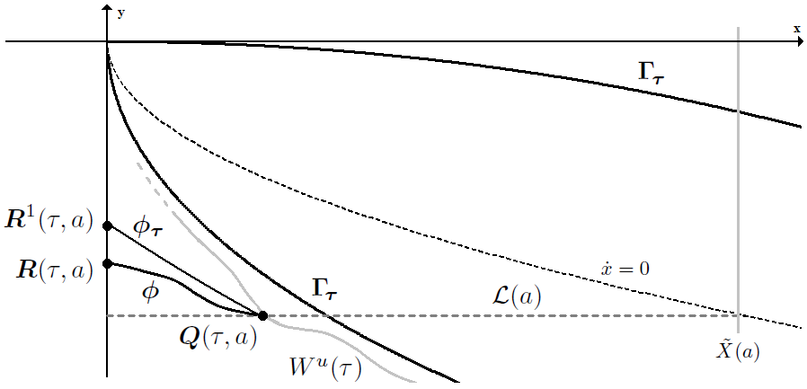
From Proposition 21, there exists such that crosses the negative semi-axis at in a point, say (see Figure 4)
(38)
According to Remark 25, it is not restrictive to assume that for any
(provided that we choose in Remark 27).
So, from Lemma 9 we deduce that .
Figure 4: The position of the points , , and .
Our next purpose is to provide suitable estimates from above and from below of .
From Lemma 28,
is a graph on the -axis when .
In particular,
we can find a function such that the image of can be parametrized as for .
Let us now consider the trajectory of the system (15) frozen at .
Notice that its graph is contained in the level set
(39)
which lies in the exterior of the homoclinic orbit defined in (19).
Hence, there exists
such that lies in the quadrant when and it crosses transversely the negative semi-axis at
in a point, say (see Figure 4)
(40)
Remark 29.
Assume , then the functions and are continuous in their domain since the flow on the negative -axis is transversal.
From the study of the trajectories of the autonomous system (15),
we can deduce that
(41)
and, consequently,
we can find a strictly decreasing function such that the image of can be parametrized as for .
Lemma 30.
Assume and that for any .
Fix ,
and let be as in Remark 27. Then,
Proof.
For brevity, let us write
and
.
From (16) combined with Lemma 28,
we see that is strictly increasing in the interval . In particular,
recalling (39), we have
for every and .
Thus,
we get
(42)
and, as an immediate consequence,
The statement of the lemma holds if we prove that for any .
Observe first that . Then, from (11) and (15)
we find that equals along with its first and second derivatives, however
Hence, when is in a suitable right neighborhood of .
Let
If ,
the lemma is proved. So, we assume by contradiction that . Then, we have ,
and .
Hence, recalling (42),
So in a left neighborhood of ,
giving a contradiction.
∎
In the following Lemma we assume bounded. This assumption will be removed via Remark 25.
Lemma 31.
Assume , , and .
For any we define
(43)
Then, there is such that, for any ,
(44)
(45)
Proof.
Let be the value provided by Remark 27, and fix .
We consider again the trajectories
and
.
Observe that along the horizontal segment . as well as in the interior of the bounded set enclosed by , and the negative semi-axis. Using this fact, according to Lemma 28 and
(41), we see that
for any and any .
Moreover, for both the trajectories we get
Assume , and that for any .
If , then there exists
such that
Proof.
We simply need to choose in Lemma 33 satisfying the
assumption .
Then, we set as in (43), so that Lemma 33 permits us to
conclude the proof recalling that by Lemma 30.
∎
Proposition 35.
Assume , and that for any .
If , then there exists such that
and .
Proof.
Let be as in Proposition 34.
Then, we can recover the constant provided by Remark 27, and the function defined in Lemma 20 such that .
From Lemma 20
there exists such that
the inverse function
is continuous and satisfies
.
In particular, .
Since the previous results focus their attention
on a neighborhood of , recalling Remark 25 we can
remove the hypothesis and the monotonicity assumption on .
Proposition 36.
Assume .
If , then there exists
such that
Now, repeating the argument of the proof of Proposition 35 combined with the truncation argument of the proof of Proposition 36, we
obtain the asymptotic behavior of for large values of , which will allow us to prove
the part of Theorem 1 concerning the case.
Proposition 37.
Let assumption hold with . Then, there exists such that
and .
4.2 The case .
In this subsection we focus our attention on the opposite case .
We invite the reader to take in mind Lemma 20, i.e.
the intersection time if and only if .
Remark 38.
Recalling the definition of in (2)
we see that if then
(56)
Lemma 39.
Let assumptions , , and hold with . Let us fix
and define as in (43).
Assume that there exists a sequence with , satisfying .
Then, if is sufficiently large,
Proof.
Since both and converge to ,
according to Remark 25,
we can set
for every .
Then, using (14), (46), Remark 32 and (56), we get
when is sufficiently large.
We argue by contradiction, and assume that there exists a subsequence of , still called for simplicity, which satisfies
so that, for sufficiently large ,
Then, recalling the definition of in (13) and the definition of in (38), we get
where . Hence,
setting ,
from (44) and (55)
it follows that
which contradicts our assumption .
∎
Lemma 40.
Let assumption hold with . Fix and define
(57)
Let us assume that there exist a sequence with , such that .
Then, if is sufficiently large,
Proof.
Arguing as in Remark 25, we can modify system (11), replacing with and notice that we can apply Lemma 39 in this case.
From the hypothesis, we deduce that, for large, we have . Since
and the original coincide on , we easily conclude.
∎
where we set , if the corresponding trajectory does not cross the negative -axis.
Proof.
We argue by contradiction assuming
the existence of a sequence , with and satisfying .
Since we are focusing our attention on a neighborhood of , we can again suitably modify in the function as suggested in Remark 25, in order to ensure the validity of the hypotheses of Lemma 39.
Hence, we can assume,
without loss of generality, that and hold, too.
So, according to (14), the energy is increasing along the trajectories.
As a consequence, from Lemma 40 and Remark 27, we get
for sufficiently large.
So, recalling
the definition of in (13) and the definition of in (38),
we can find a positive constant such that
Moreover, we can use the estimate in Remark 32 to get
for sufficiently large. Hence, we have
leading to
which is in contradiction with
.
The proposition is thus proved.
∎
When (with the strict inequality), we find a more precise estimate.
Assume that there is such that, for every , there exists a time at which the trajectory
crosses the negative semi-axis, and
for any .
Then
Proof.
Let , given by Proposition 41.
Without loss of generality, we choose
the value provided by Remark 25 so that .
Recalling Remark 38, we first fix satisfying
(58)
and then such that
Since , we can introduce
such that
(59)
Consider the trajectory of system (11) departing from at the time and the points
When we focus our attention on the trajectory restricted to the interval , recalling the truncation argument in Remark 25, we can assume that both and hold.
So, we can argue as in the proof of Lemma 39,
to obtain such that
Assume by contradiction that there is and a sequence such that and .
Let us now focus our attention on .
We remark that the validity of and is not guaranteed anymore in ;
however , so in this interval. Hence, we can compute
Theorem 2 follows from Proposition 43, cf. §5 for more details.
In order to prove the second part of Theorem 1, we need to remove
the monotonicity assumption from Proposition 43.
Note that if does not hold, we cannot ensure
the existence of points of in a neighborhood of ,
when .
However, we can prove a weaker result.
Proposition 44.
Assume , and define
If , then there is such that for any .
Proof.
Fix , as in (57) and set as in Remark 27.
Let be as in Remark 25.
From Proposition 41 we deduce that
(66)
Now, let us fix and denote by the branch of the unstable manifold between the origin and
. From Remark 17 we see that there is such that the function
restricted to gives a parametrization of , i.e.
is a continuous bijective function.
Using Remark 14 and Lemma 16, reducing if necessary, we see that if then
is close to the corresponding trajectory in when ; in particular
if . Hence for any .
Let now . Recalling Remark 17, we have , and using
Lemma 20 we see that there is a unique
such that the trajectory
crosses transversely at .
Then, from (66) we see that
Hence for any .
Then, setting , the Proposition is proved.
∎
Now, we reprove Proposition 43 by replacing the global assumption with the local assumption .
Motivated by [3, 7, 39],
and inspired by [18] and [22], we obtain the following result.
Lemma 45.
Assume with ; assume further either or that
there is such that when .
Then, there is such that .
Notice that if with holds and exists and it is positive, either bounded or
unbounded, or if is asymptotically periodic, then Lemma 45 applies.
The proof of Lemma 45 is rather technical and it is postponed to Section 4.2.1, as well as the related proof of the following adapted version of Proposition 43.
Proposition 46.
Assume with ; assume further either or that
there is such that when .
Then
We start by proving Lemma 45 under assumption :
the following arguments are preliminary to the proof under this hypothesis.
The alternative case where it is assumed that is then obtained as a Corollary.
Let us assume , so that we can construct the stable manifold , see §2 and, in particular, (23).
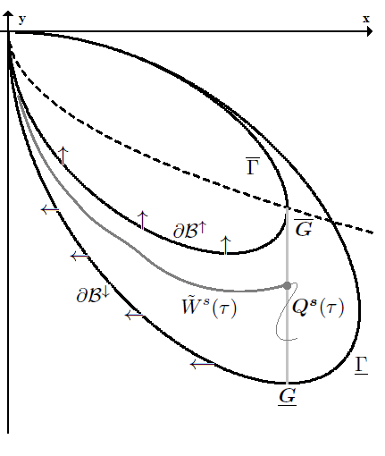
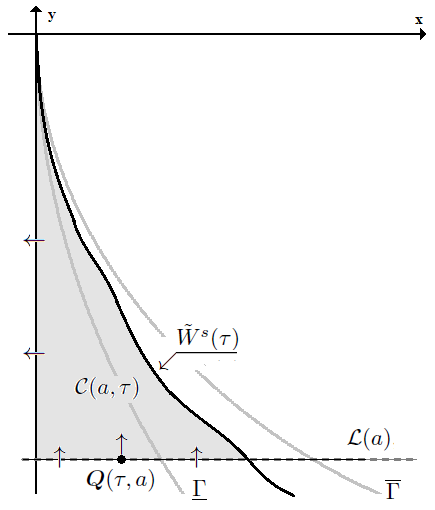
To develop our construction we need to define several sets, and we invite the reader to follow the argument on Figure 5.
Assume and , then
for any we set
We define and
. Notice that both and are the image
of closed regular curves; we denote by and by the bounded sets enclosed by
and , respectively: notice that .
We denote by the (transversal) intersection between and the isocline such that .
Then, we denote by the intersection between the line and contained in and by
the vertical segment between and . Moreover, we denote by the branch of
between the origin and contained in
and by the branch of
between the origin and contained in .
Finally, we denote by the compact set enclosed by , and , see Figure 5.
We emphasize that if is a trajectory of (11), we find,
according to (16),
Using this fact, we easily obtain the following crucial remark
Remark 47.
Assume and , then the flow of (11) on
aims towards the interior of for any , while on
aims towards the exterior of for any .
Figure 5: The constructions needed in the proof of Lemma 45
Let us now fix . From Remark 47 and the construction in §2,
we see that
intersects (not necessarily transversely), see [22, Lemma 2.8].
Follow from the origin towards : denote by the first intersection with
and by the connected branch of between the origin and .
In what follows, we recall the argument in [22, pp. 357–360].
Let us consider the autonomous systems (11), where is replaced by , respectively , and we denote by
the trajectories of these systems starting at time from the point .
From (20), recalling that in the region the branch of
lies under the corresponding branch of ,
see Figure 5,
we can find such that
or, equivalently,
(70)
Such estimates permit us to provide analogous ones for the solutions of the non-autonomous system (11).
We give the proof of the first inequality, the other being similar. Let . Assume by contradiction that . Then, and since , from (68) and Remark 47
the trajectory remains in the interior
of and in particular we get .
So, from (11) and (15), we deduce that
, providing in a right neighborhood of , leading to a contradiction.
∎
From Lemma 48, we obtain the following result, which has already been proved in [22, Lemma 3.1] focusing the attention on the point , but we repeat the argument here to correct some typos.
Lemma 49.
Assume and with .
Then, there is such that
for any and .
Take any and consider a point .
We denote, for brevity, the trajectory as .
We note that must cross the line
at a time smaller than .
So, let us denote by the largest value with such a property. In particular, by construction, ,
and for every .
Using Lemma 48, we have
(72)
Since we see that
is decreasing in the interval ; so using (72),
From Remark 27, there is such that intersects transversely in a point
denoted by , for every . Moreover,
since , a subsegment of joins with (transversely), and, consequently,
from the previous argument,
intersects , too, for every .
Lemma 50.
Assume and with .
Then, there is such that for any the trajectory
corresponds to a crossing solution, i.e. there is such that
for any and it becomes null at . Further
for any .
Proof.
Let us consider the compact set , see Figure 5, delimited by ,
the negative semi-axis and the line , for any .
Then, from Remark 27, we can find , with provided by Lemma 49, such that
Fix ; then by construction , when
is in a sufficiently small right neighborhood of , see Remark 13.
So, there is such that for any
and it leaves when , or for any
(i.e. ).
From an analysis of the phase portrait we see that
(75)
Assume first that , then either crosses the negative semi-axis at
proving the thesis, or .
So, assume the latter and observe that
, thus .
Then, for any , and by construction
for any . So, since the trajectories and coincide, we conclude that
for any , thus giving us .
Hence, we get a contradiction comparing (74) with Lemma 49.
We consider now the remaining case: . Recalling (75), the only reasonable conclusion is that as , i.e. .
Whence, from (75) we find
, and get again the contradiction comparing (74) with Lemma 49.
So, the lemma is proved.
∎
Taking advantage of this result, we can extend it to a wider class of functions.
Lemma 51.
Assume with , and that
there is such that when .
Then, the same conclusion as in Lemma 50 holds.
Proof.
Recalling that , by assumption there is
such that when .
Let us define
Let
be the trajectory
of the modified system (11) where is replaced by .
Observe that satisfies and we can still apply Remark 13, but depends continuously and not smoothly on .
Since the original system and the modified one coincide for , then their unstable manifolds are the same in this interval.
Concerning the modified system, let
and select the point as above.
Then, from Remark 27 we see that for any , cf. (73), there is , such that crosses transversely in for any .
From Lemma 50
applied to the modified system,
we can find such that for any there are and
such that
and both
and
hold for any , see (75).
Since for any , if , the thesis is achieved. So, we assume ; since is constant then is constant when , see (16), then
for any .
Let us set
, then from the previous estimate we get .
Notice that we can rewrite the image of as a graph in , i.e. there is a decreasing smooth function such that
for every .
Therefore
we see that the trajectory is forced to stay in the unbounded set
whenever .
Observe now that the maximum of within is obtained in which is compact; further it has to be negative, so there is
such that when .
Then it is easy to check that is bounded when .
So, from elementary considerations, we see that crosses the negative semiaxis at .
∎
The previous lemmas permit us to complete the proof of Lemma 45.
We fix as in (73), and consider the segment defined as in (36).
From Remark 27, there is such that intersects in for every .
Using Lemma 20, we consider the decreasing continuous function
such that the solution of (4) corresponds to the trajectory of (11).
Then, either Lemma 50 or 51 applies providing the value such that the solution is a crossing solution for every . Setting such that ,
we get . The lemma is thus proved.
∎
Take such that defined in (57) satisfies the inequality
(73). Define the segment as in (36), and , as in
Lemma 50 or 51. Set as in the proof of Lemma 45.
Recalling Lemmas 20 and 45,
we have and . Moreover, the function is well defined in , and it is continuous, cf. Remark 29.
Hence, we are able to apply Proposition 42 to infer (65).
∎
5 Proof of the theorems
Since all the preliminaries are well-established, we conclude our paper by giving the explicit proof of our main theorems.
If , from Proposition 37 there is such that and .
So, there is such that and ; whence from Propositions 23 and 24
we have . Further,
since is continuous in , see Proposition 22, we find : i.e.
for every there is such that , which amounts to say that solves problem (3).
The second assertion
follows immediately from Proposition 44.
∎
The proof takes advantage of Propositions 23 and 43.
If , we distinguish two alternatives: either where is an internal minimum of or
where .
Then, the proof is concluded.
On the other hand, if ,
from , we deduce that the function has an internal minimum , and
the pre-image has at least two elements for every , thus giving the multiplicity result.
∎
Remark 52.
We want to underline that in the critical case we are not able to discern which of the alternatives analyzed in the proof of Theorem 2 holds, and, consequently,
we are not able to say if there is a solution for .
From Proposition 44 and Lemma 45, the set contains a nontrivial interval, and there exists .
Then, the proof follows the lines of the one of Theorem 2, profiting from
Propositions 22, 23, 24 and 46.
∎
Acknowledgements
Francesca Dalbono was partially supported by the PRIN Project 2017JPCAPN “Qualitative and quantitative aspects of nonlinear PDEs” and by FFR 2022-2023 from University of Palermo.
All the authors are members of INdAM-GNAMPA.
References
[1]
Bamón R., Flores I., del Pino M., Ground states of semilinear elliptic equations: a geometric approach,
Ann. Inst. H. Poincaré Anal. Non Linéaire, 17 (2000), 551-581.
[2]
Battelli F., Johnson R., Singular ground states for the scalar curvature equation in , Differential Integral Equations, 14 (2001), 141-158.
[3]
Bianchi G., Egnell H.,
An ODE approach to the equation , in ,
Math. Z., 210 (1992), 137-166.
[4]
Bidaut-Véron M.F., Local and global behavior of solutions of quasilinear equations of Emden-Fowler type,
Arch. Rational Mech. Anal., 107 (1989), 293-324.
[5] H. Brezis, L. Nirenberg, Positive solutions of nonlinear elliptic equations involving critical Sobolev exponents, Comm. Pure Appl. Math., 36 (4) (1983), 437-477
[6] C. Budd, J. Norbury, Semilinear elliptic equation and supercritical growth, J. Differential Equations
68, (1987) n. 2, 169-167.
[7]
Chen C.C., Lin C.S.,
Estimates of the conformal scalar curvature equation via the method of moving planes,
Comm. Pure Appl. Math., 50 (1997), 971-1017.
[8]
Chen C.C., Lin C.S.
Blowing up with infinite energy of conformal metrics on ,
Comm. Partial Differential Equations, 24 (1999), 785-799.
[9]
Cheng K.S., Chern J.L., Existence of positive entire solutions of some semilinear elliptic equations, J.
Differerential Equations, 98 (1992), 169–180.
[10]
Chtioui H., Hajaiej H., Soula M.,
The scalar curvature problem on four-dimensional manifolds,
Commun. Pure Appl. Anal., 19 (2020), 723-746.
[11]
Coddington E., Levinson N., Theory of Ordinary Differential Equations. Mc Graw Hill, New York, 1955.
[12]
Dalbono F., Franca M., Nodal solutions for supercritical Laplace equations, Commun. Math. Phys., 347 (2016), 875-901.
[13]
Deimling K., Nonlinear functional analysis. Springer, Berlin, 1985.
[14]
Ding, W.Y., Ni, W.M., On the elliptic equation and related topics, Duke Math. J., 52 (1985), 485-506.
[15] J. Dolbeault, I. Flores, Geometry of Phase space and solutions of semilinear elliptic
equations in a ball, Trans. Am. Math. Soc. 359, (2007) n. 9, 4073-4087
[16] (MR3373577) [10.1016/j.na.2015.04.015]
I. Flores and M. Franca,
Phase plane analysis for radial solutions to supercritical quasilinear elliptic equations in a ball,
Nonlinear Anal., 125 (2015), 128-149.
[17]
Fowler R.H., Further studies of Emden’s and similar differential equations, Q. J. Math., 2
(1931), 259-288.
[18]
Franca M., Non-autonomous quasilinear elliptic equations and Ważewski’s principle,
Topol. Methods Nonlinear Anal., 23, (2004), 213-238.
[19]
Franca M., Corrigendum and addendum to “Non-autonomous quasilinear elliptic equations and Ważewski’s principle”, Topol. Methods Nonlinear Anal., 56 (2020), 1-30.
[20]
Franca M., Classification of positive solution of -Laplace
equation with a growth term, Arch. Math. (Brno), 40, (2004), 415-434.
[21]
Franca M., Fowler transformation and radial solutions for quasilinear elliptic equations. I. The subcritical and the supercritical case,
Can. Appl. Math. Q. 16 (2008), 123-159.
[22]
Franca M., Structure theorems for positive radial solutions of the generalized scalar curvature
equation, Funkcial. Ekvac., 52 (2009), 343-369.
[23]
Franca M., Johnson R., Ground states and singular ground states for quasilinear partial differential equations with
critical exponent in the perturbative case, Adv. Nonlinear Stud., 4 (2004), 93-120.
[24]
Franca M., Sfecci A., Entire solutions of superlinear problems with indefinite weights and Hardy potentials, J. Dynam. Differential Equations, 30 (2018), 1081-1118.
[25]
Franchi B., Lanconelli E., Serrin J., Existence and uniqueness of
nonnegative solutions of quasilinear equations in , Adv. Math., 118 (1996) 177-243.
[26]
García-Huidobro M., Manásevich R, Yarur C.S.,
On the structure of positive radial solutions to an equation containing a -Laplacian with weight,
J. Differential Equations, 223 (2006), 51-95.
[27]
Gazzola F.,
Critical exponents which relate embedding inequalities with quasilinear elliptic problems,
Discrete Contin. Dyn. Syst., suppl. (2003), 327-335.
[28] Z. Guo, J. Wei, Global solution branch and Morse index estimates of a semilinear
elliptic equation with super-critical exponent, Trans. Amer. Math. Soc., 363, (2011) n. 9, 4777-4799.
[29]
Johnson R., Concerning a theorem of Sell, J. Differential Equations, 30
(1978), 324-339.
[30]
Johnson R., Pan X.B., Yi Y.F.,
Singular ground states of semilinear elliptic equations via invariant manifold theory,
Nonlinear Anal., 20 (1993), 1279-1302.
[31]
Johnson R., Pan X.B., Yi Y.F., The Melnikov method and elliptic equation with critical exponent,
Indiana Univ. Math. J., 43 (1994), 1045-1077.
[32]
Jones C., Küpper T., On the infinitely many solutions of a semilinear elliptic equation,
SIAM J. Math. Anal., 17 (1986), 803-835.
[33]
Kabeya Y., Yanagida E., Yotsutani S.,
Existence of nodal fast-decay solutions to in ,
Differential Integral Equations, 9 (1996), 981-1004.
[34]
Kawano N., Ni W.M., Yotsutani S.,
A generalized Pohozaev identity and its applications,
J. Math. Soc. Japan, 42 (1990), 541-564.
[35]
Kawano N., Satsuma J., Yotsutani S.,
Existence of positive entire solutions of an Emden-type elliptic equation,
Funkcial. Ekvac., 31 (1988), 121–145.
[36]
Kusano T., Naito M., Oscillation theory of entire solutions of second order superlinear elliptic equations,
Funkcial. Ekvac., 30 (1987), 269-282.
[37]
Li Y.Y., Prescribing scalar curvature on and related problems, Part II: Existence and compactness,
Comm. Pure Appl. Math., 49 (1996), 541-597.
[38]
Li Y.Y., Nguyen L., Wang B.,
The axisymmetric -Nirenberg problem, J. Funct. Anal., 281 (2021), Paper N. 109198, 60 pp.
[39]
Lin C.S., Lin S.S.,
Positive radial solutions for in and related topics,
Appl. Anal., 38 (1990), 121-159.
[40] F. Merle, L.A. Peletier, Positive solutions of elliptic equations involving supercritical growth, Proc. Roy.
Soc. Edinburgh sect A, 118, (1991), 49-62.
[41]
Ni W.M.,
On the elliptic equation , its generalizations, and applications in geometry,
Indiana Univ. Math. J., 31 (1982), 493-529.
[42]
Ni W.M., Serrin J.,
Nonexistence theorems for quasilinear partial differential equations,
Rend. Circ. Mat. Palermo (2), 8 (1985), 171-185.
[43]
Sharaf K., A note on a second order PDE with critical nonlinearity,
Electron. J. Qual. Theory Differ. Equ., 10 (2019), 16 pp.
[44] Yanagida E., Yotsutani S.,
Classification of the structure of positive radial solutions to in ,
Arch. Rational Mech. Anal., 124 (1993), 239-259.
[45]
Yanagida E., Yotsutani S., Existence of nodal fast-decay solutions to
in , Nonlinear Anal., 22 (1994), 1005-1015.