Reasoning Limitations of Multimodal Large Language Models. A case study of Bongard Problems

Abstract

Abstract visual reasoning (AVR) encompasses a suite of tasks whose solving requires the ability to discover common concepts underlying the set of pictures through an analogy-making process, similarly to human IQ tests. Bongard Problems (BPs), proposed in 1968, constitute a fundamental challenge in this domain mainly due to their requirement to combine visual reasoning and verbal description. This work poses a question whether multimodal large language models (MLLMs) inherently designed to combine vision and language are capable of tackling BPs. To this end, we propose a set of diverse MLLM-suited strategies to tackle BPs and examine four popular proprietary MLLMs: GPT-4o, GPT-4 Turbo, Gemini 1.5 Pro, and Claude 3.5 Sonnet, and four open models: InternVL2-8B, LLaVa-1.6 Mistral-7B, Phi-3.5-Vision, and Pixtral 12B. The above MLLMs are compared on three BP datasets: a set of original BP instances relying on synthetic, geometry-based images and two recent datasets based on real-world images, i.e., Bongard-HOI and Bongard-OpenWorld. The experiments reveal significant limitations of MLLMs in solving BPs. In particular, the models struggle to solve the classical set of synthetic BPs, despite their visual simplicity. Though their performance ameliorates on real-world concepts expressed in Bongard-HOI and Bongard-OpenWorld, the models still have difficulty in utilizing new information to improve their predictions, as well as utilizing a dialog context window effectively. To capture the reasons of performance discrepancy between synthetic and real-world AVR domains, we propose Bongard-RWR, a new BP dataset consisting of real-world images that translates concepts from hand-crafted synthetic BPs to real-world concepts. The MLLMs’ results on Bongard-RWR suggest that their poor performance on classical BPs is not due to domain specificity but rather reflects their general AVR limitations.

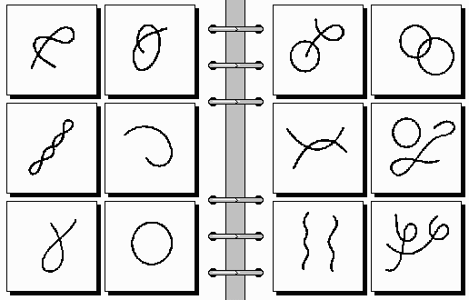
(a) Bongard Problem #31 (Bongard, 1970)

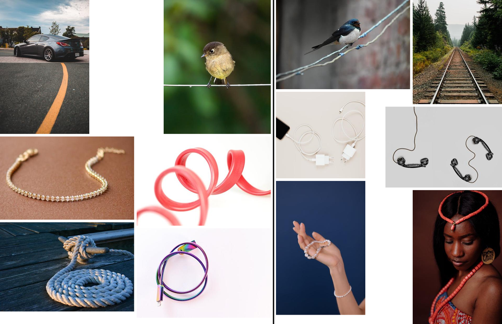
(b) Bongard-RWR (This work)

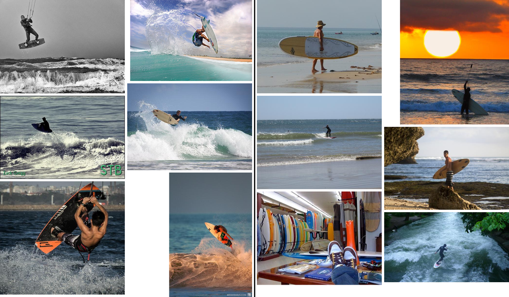
(c) Bongard HOI (Jiang et al., 2022)

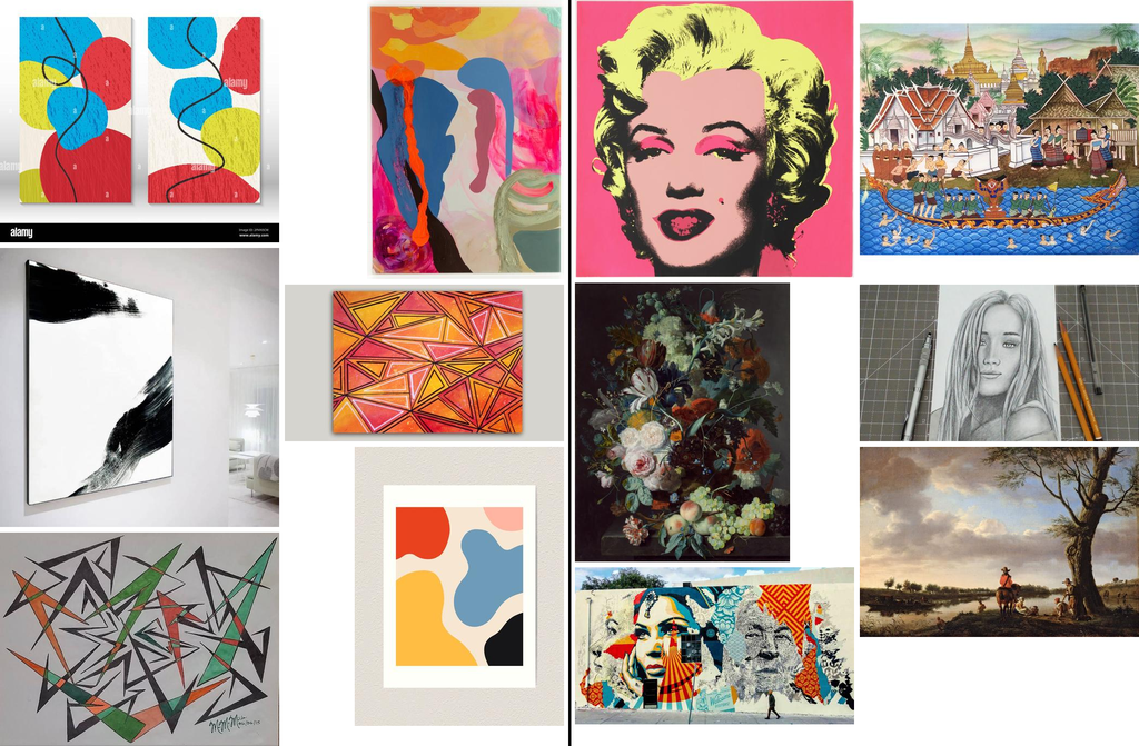
(d) Bongard-OpenWorld (Wu et al., 2024)

Figure 1: Bongard Problems. In this work, we consider BPs with both synthetic and real-world images. (a) A manually designed BP #31. Left: One line. Right: Two lines. (b) A real-world representation of BP #31 from the proposed Bongard-RWR dataset introduced in Section 4. Left: One line. Right: Two lines. (c) Bongard HOI: Left: A person jumping on a surfboard. Right: Not a person jumping on a surfboard. (d) Bongard-OpenWorld: Left: An abstract painting. Right: Not an abstract painting. Descriptions of the Left / Right sides come from the respective datasets.

1 Introduction

Analogy-making is a critical aspect of human cognition, tightly linked with fluid intelligence, the capacity to apply learned skills in novel settings (Lake et al., 2017). Several approaches have been proposed to build systems capable of making analogies. Notably, the structure-mapping theory explores methods for discovering structural correspondences between pre-existing object representations (Winston, 1982; Gentner, 1983; Carbonell, 1983; Falkenhainer et al., 1989; Holyoak & Thagard, 1989). However, these approaches often overlook the perceptual aspect, assuming object representations are already given. Chalmers et al. (1992) highlight that forming useful representations is an intricate challenge. In particular, perception is not merely a passive reception of sensory data, but rather an active interpretation influenced by prior knowledge. This process involves the detection of patterns, recognition of analogies, and abstraction of concepts. The resultant representations may vary significantly depending on the context, which underscores the importance of modeling perception and cognition jointly (Hofstadter, 1995).

Multiple problems that necessitate combined perception and reasoning have been identified (Hofstadter, 1999). Among these tasks are Bongard Problems (BPs), introduced by Bongard (1968; 1970). Initial BPs were designed manually, leading to the formulation of a few hundred task instances by individual contributors (Foundalis, 2006b). A typical BP consists of two sides, left and right, each comprising six image panels arranged in a grid. All images on one side illustrate a shared concept absent in the images on the opposite side. The task is to identify the underlying rule that differentiates the sides and articulate it in natural language. Initial BPs (Bongard, 1968), akin to human IQ tests, featured abstract 2D geometric shapes, putting the focus on abstract reasoning. However, recent works have expanded the set of BPs to include real-world images, which broadens the scope of presented objects, attributes and relations. Specifically, the matrices in Bongard HOI (Jiang et al., 2022) depict human-object interactions, while Bongard-OpenWorld (Wu et al., 2024) employs open-world free-form concepts, increasing the diversity of featured scenes. Figs. 1(a), 1(c), 1(d) illustrate examples of problems from the three above-mentioned datasets.

A central theme in BPs is recognition of concepts in a context-dependent manner, as object representations need to be formed specifically for the presented matrix, rather than described a priori (Linhares, 2000). For example, consider the matrix in Fig. 1(a) – an analysis restricted to its left side may yield multiple concepts, such as the presence of curves or an object centered in the image. Only through a comprehensive understanding of both matrix sides one can recognize that the left side depicts a single line, while the right side presents two lines. Such concept-based tasks were argued to promote a more accurate evaluation of a system’s generalization ability and its capacity for abstraction (Mitchell, 2021; Odouard & Mitchell, 2022). Moreover, the concepts in BPs are illustrated with several image examples, which positions the task within a few-shot learning setting (Fei-Fei et al., 2006; Wang et al., 2020). In contrast to other abstract reasoning problems, such as Raven’s Progressive Matrices (RPMs) (Raven, 1936; Raven & Court, 1998; Małkiński & Mańdziuk, 2022) that have recently witnessed the development of large-scale benchmarks (Barrett et al., 2018; Zhang et al., 2019), BPs allow to assess system’s ability to derive concepts from a limited set of examples (typically six images per matrix side). The above aspects make BPs a valuable testbed for assessing abstract reasoning abilities of AI models.

Motivation.

The quest to build systems capable of forming abstract concepts dates back to the 1950s (McCarthy et al., 2006). The advent of Deep Learning (DL) opened new possibilities to tackle BPs (Kharagorgiev, 2018; Nie et al., 2020). However, despite significant advancements, methods for consistently solving BPs (and other problems that involve abstract reasoning) are still lacking (Mitchell, 2021; van der Maas et al., 2021; Stabinger et al., 2021). Typically, DL approaches omit the generation of natural language answers by casting BP into a binary classification task, in which a test image had to be assigned to the matching side of the matrix. Conversely, a parallel stream of research on large language models (LLMs) demonstrated promising results in open-ended language generation (Brown et al., 2020). In particular, LLMs were applied to selected AVR tasks (Webb et al., 2023), though, lately Xu et al. (2024a) pointed certain LLM limitations in solving AVR problems represented as text despite using information lossless translation through direct-grid encoding. Recent works have combined the vision and language modalities into multimodal large language models (MLLMs) (Achiam et al., 2023; Reid et al., 2024; Anthropic, 2024), inviting their application to diverse tasks (Yin et al., 2023; Wu et al., 2023). Motivated by these recent developments we examine the reasoning capabilities of MLLMs in solving BPs.

Contributions.

The main contribution of this paper is four-fold.

(1) For the first time in the literature, we consider BPs in the context of MLLMs and propose a diverse set of strategies to solve BP instances in two setups: open-ended language generation and binary classification.

(2) We evaluate $4$ state-of-the-art proprietary MLLMs and $4$ open MLLMs on both synthetic and real-world BPs, and identify their severe abstract reasoning limitations.

(3) To further examine the main difficulties faced by MLLMs in solving both types of BPs (synthetic and real world ones) we introduce a focused dataset of BPs (Bongard-RWR) comprising real-world images that represent concepts from synthetic BPs using real world images. Thanks to relying on the same abstract concepts as synthetic BPs, Bongard-RWR facilitates direct comparisons of the MLLMs performance in both domains.

(4) We perform a detailed comparative analysis of $8$ MLLMs on Bongard-RWR vs. synthetic BPs, shedding light on the reasons of their generally poor performance.

2 Related Work

AVR tasks.

The AVR field encompasses a broad set of problems aimed at studying various aspects of visual cognition (Gardner & Richards, 2006; Małkiński & Mańdziuk, 2023). Recent DL research in this domain gravitated towards utilizing certain well-established datasets, e.g. with visual analogies (Hill et al., 2019; Webb et al., 2020) or RPMs (Zhang et al., 2019; Barrett et al., 2018), to measure the progress of DL models. However, such benchmarks evaluate system performance in learning a particular task, rather than assessing its general ability to acquire new AVR skills. To address this limitation, certain tasks have adopted few-shot learning setups, requiring models to learn from a few demonstrations, as exemplified by SVRT (Fleuret et al., 2011) or Bongard-LOGO (Nie et al., 2020). Nonetheless, these benchmarks follow a discriminative setting where a set of possible answers is provided. Conversely, other datasets such as ARC (Chollet, 2019) or PQA (Qi et al., 2021) pose a generative challenge, which may be considered more difficult due to its open-ended nature. In addition to synthetic tasks featuring 2D geometric shapes, certain datasets present analogous reasoning tasks using real-world images (Teney et al., 2020; Ichien et al., 2021; Bitton et al., 2023). This approach extends the range of concepts that can be expressed and, above all, allows employing models pre-trained on large image datasets. In this work, we concentrate on several BP datasets that present a few-shot learning challenge, cover both synthetic and real-world images, and consider settings involving both binary classification and answer generation in natural language.

Approaches to solve BPs.

Initial approaches to tackle BPs involved cognitive architectures (Foundalis, 2006a), program synthesis coupled with inductive logic programming (Saito & Nakano, 1996; Sonwane et al., 2021), and the application of Bayesian inference within a visual language framework (Depeweg et al., 2018; 2024). Kharagorgiev (2018) trained a convolutional network on a generated synthetic dataset with geometric shapes and applied a one-level decision tree to solve BPs framed as a binary classification task. Nie et al. (2020) introduced Bongard-LOGO with synthetically generated BPs and used it to evaluate CNN-based models focused on meta-learning (Snell et al., 2017; Mishra et al., 2018; Lee et al., 2019; Raghu et al., 2020; Chen et al., 2021) and relational reasoning (Barrett et al., 2018). Jiang et al. (2022) applied the Relation Network (Santoro et al., 2017) to objects detected with Faster R-CNN (Ren et al., 2015) and employed the model to solve matrices from the real world Bongard HOI dataset. Despite high diversity of approaches, none of them has fully addressed the abstract and open-ended nature of BPs. Most related to our work, Wu et al. (2024) considered hybrid approaches that caption each image panel with an image-to-text model and applied LLMs for processing these text descriptions. Differently, in this work we focus on MLLMs that are inherently capable of jointly processing images and text.

Abstract reasoning of MLLMs.

MLLMs haven’t been yet applied to tackle BPs, though they were applied to several related tasks. Initial works focused on LLMs and evaluating their abstract reasoning performance in simplified analogy tasks. Webb et al. (2023) showed that GPT-3 and GPT-4 (text-only variants) performed on the human level, or even outcompeted humans, in certain RPM-like tasks in a zero-shot manner without additional fine-tuning. However, they represented the image objects as text using a fixed small vocabulary, thus omitting the need for identifying concepts from open-ended shapes, a key challenge of BPs. Recent research concerning the evaluation of abstract reasoning skills of LLMs concentrates around the Abstraction and Reasoning Corpus (ARC) task (Chollet, 2019). It was demonstrated that LLMs can solve certain ARC problems transformed to the text domain (Moskvichev et al., 2023; Mirchandani et al., 2023; Camposampiero et al., 2023; Xu et al., 2024b). Despite these important stepping stones, the text-based representation taken in these works simplifies the perception task by presenting the model with pre-existing higher level representations. Only recently, thanks to the appearance of MLLMs, vision and text started to be treated jointly in a unified manner. Cao et al. (2024) proposed a suite of AVR tasks to compare MLLM and human performance. Jiang et al. (2024) assessed AVR skills of MLLMs on an introduced multidimensional benchmark combining AVR and perceptual questions. Our work complements this stream of research by exploring BPs, a fundamental task in the field, and providing insights into MLLM analogy-making performance in synthetic and real-world domains.

Figure 2: Generation strategies. Direct (a) feeds the image of the whole matrix to the model. Descriptive (b), Contrastive (d), and their iterative variants, (c) and (e), present individual image panels to the model in a fixed order. Their direct variants, (b) and (d), additionally include the image of the whole matrix. Grey background marks a sequence of requests run in a single context window.

3 Solving BPs with MLLMs

In this paper, we propose a set of novel strategies for solving BPs using MLLMs. Definition of each strategy includes the input on which the model operates and the sequence of reasoning steps performed by the model. A high-level overview of these methods is provided in Fig. 2. In the main tested setting, we follow the initial BP formulation that requires providing an answer in natural language, and propose a model-based approach to automatically evaluate such model predictions. In addition, we consider simpler formulations of the problem, casting it into a binary classification framework that enables detailed evaluation of AVR abilities of the tested MLLMs. An illustration of these evaluation settings is presented in Fig. 3. In what follows, let ${\cal BP}^{X}=\{{\cal L}^{X},{\cal R}^{X},y^{X}\}$ denote a BP instance ($X\in\cal N$ is an index), composed of ${\cal L}^{X}=\{L^{X}_{1},\ldots,L^{X}_{6}\}$ left and ${\cal R}^{X}=\{R^{X}_{1},\ldots,R^{X}_{6}\}$ right panels, resp., and its concept $y^{X}$ expressed in natural language.

3.1 Prompting Strategies for Natural Language Answer Generation

We start by defining the strategies for generating answers in natural language. In each strategy, the model receives a general description of Bongard Problem with two BP examples with correct answers. Additionally, besides this generic introductory information, a given task ${\cal BP}^{X}$ to be solved is presented in a strategy-specific way. Appendix A.4 presents the exact prompt formulations.

Direct (Fig. 2a). The model receives an image presenting ${\cal BP}^{X}$ and is asked to directly formulate an answer (i.e., describe the difference between ${\cal L}^{X}$ and ${\cal R}^{X}$ panels in natural language).

Descriptive (Fig. 2b). Defines a more granular approach in which the model is first requested to generate a textual description of each image panel of the matrix. Each description is generated in a separate context, such that the model doesn’t have access to the prior panels nor to their descriptions. Next, the model is requested to provide an answer to the problem based only on the generated textual descriptions of all image panels.

Descriptive-iterative (Fig. 2c). Evaluates the role of the reasoning context and utilizes a context window comprising the dialog history concerning all images in the given side of the problem. After generating the description of the first image, the model iteratively refines its output based on subsequent images from the same side. Based on the textual descriptions of both sides of the problem, the model is requested to provide the final answer.

Descriptive-direct (Fig. 2b with a dashed element). In both above Descriptive strategies, the model is never presented with the image of the whole matrix ${\cal BP}^{X}$. Descriptive-direct strategy extends Descriptive by providing the image of ${\cal BP}^{X}$ along with the textual panel descriptions.

Contrastive (Fig. 2d). A critical aspect of BPs is the focus on forming concepts within the specific context of the matrix ${\cal BP}^{X}$. It’s often the case that correct identification of the concept governing one side requires analysis of the other side to identify their key differences. In Descriptive strategies, the model provides image descriptions concerning a single problem side ${\cal L}^{X}$ or ${\cal R}^{X}$ without taking into account the images from the other side. Conversely, in the Contrastive strategy, the model is tasked with describing the difference between a pair of corresponding images from both sides of the problem $(L^{X}_{1},R^{X}_{1}),\ldots,(L^{X}_{6},R^{X}_{6})$. After describing the differences between all six image pairs in separate contexts, the model generates its final answer based on these textual descriptions.

Contrastive-iterative (Fig. 2e). Extends Contrastive by performing all reasoning steps in a single context window, enabling the model to gradually improve its understanding of the rule separating both sides.

Contrastive-direct (Fig. 2d with a dashed element). Extends Contrastive by including the image of the whole matrix together with textual descriptions of differences within each panel pair.

Figure 3: Evaluation settings. We consider the three settings to solve BPs: (a) the ground-truth answer $y$ is paired with a description $\widehat{y}$ generated by the MLLM and the model needs to verify if they describe the same concepts; (b) given a possible solution $\overline{y}$ the model needs to assess whether it’s correct; (c) two test images corresponding to the left (L) and right (R) sides, resp., are randomly shuffled, and the model needs to assign each image from the pair to the proper side of the problem.

3.2 Evaluation of Solutions Expressed in Natural Language

The correct answer to a BP may be formulated in natural language in many different ways. To account for this inherent variability, we utilize a model-based approach to assess whether the generated answer $\widehat{y}$ matches the ground-truth $y$. In the proposed setting, an MLLM ensemble receives both $\widehat{y}$ and $y$ and is requested to output a binary yes/no answer whether both descriptions refer to the same concept (see Fig. 3a). Specifically, we assess the correctness of $\widehat{y}$ using all four considered proprietary MLLMs and count it as correct if at least two models agree with this class (see details in Appendix B). In contrast to solving the BP task, which requires abstract reasoning abilities, the task of determining whether two answers refer to the same concept boils down to assessing the semantic similarity between two texts, and MLLMs are known to excel in such setup (Lu et al., 2024).

3.3 Binary classification formulations

To dive deeper into the AVR capabilities of the studied models, we cast the BP task into three binary classification settings, reducing the task’s difficulty. Firstly, we provide the model with the image of the whole matrix ${\cal BP}^{X}$ along with a possible solution, and the model is prompted to generate a binary score assessing the correctness of the provided answer (Fig. 3b). Two settings are considered, in which the solution is formed by either the actual ground-truth answer (the expected answer is yes), or by an incorrect answer taken from a different BP matrix (the expected answer is no). Secondly, we follow a setting exemplified in the Bongard-LOGO dataset (Nie et al., 2020) in which two test images have to be classified to different sides of the problem (Fig. 3c). To this end, we take two test images corresponding to the respective sides of the matrix, randomly shuffle the images, and request the model to determine the side to which each image belongs. In synthetic BPs we create the test set by removing the 6th image from each side of the matrix, while in BPs from Bongard HOI, Bongard-OpenWorld and Bongard-RWR we use the additional test images. We refer to these three formulations as Ground-truth, Incorrect Label, and Images to Sides (see prompts in Appendix A.3).

4 Bongard-RWR: Synthetic BPs expressed in real-world images

One of the interesting research avenues is to compare the MLLMs performance on synthetic BPs vs. real-world ones. Note, however, that a direct performance comparison on synthetic Bongard dataset vs. real-world Bongard HOI and Bongard-OpenWorld datasets is not meaningful, as these datasets depict different concepts. To enable a meaningful comparison and additionally determine whether the MLLMs performance score is domain-related, we introduce Bongard Real-World Representations, a focused dataset that expresses concepts present in synthetic BPs using real-world images, thus creating their real-life equivalents, as illustrated in Fig. 1(b). Appendix C contains additional examples. The dataset is available at: https://github.com/pavonism/bongard-rwr.

4.1 Bongard-RWR dataset generation

For a given instance ${\cal BP}^{X}$, we first use GPT-4o to describe its underlying concept $y^{X}$ in $N=10$ different ways using the prompt listed in Prompt 4.1. We obtain $N$ real-world textual descriptions $D^{X}_{i}=\{D^{XL}_{i},D^{XR}_{i}\},$ $i=0,\ldots,N-1$, of each side $S\in\{L,R\}$. Then, we use image search engine Pexels API (Pexels, 2024) to download $M=15$ images per each described side $D^{XS}_{i}$. We employ GPT-4o (see Prompt  A.1 in Appendix  A.1) to select only those images that properly illustrate the concept of the respective side and are indeed distinguishable from the alternative concept. We stop the selection procedure after having a set of $T=3$ descriptions $\{D^{X}_{i_{1}},D^{X}_{i_{2}},D^{X}_{i_{3}}\}$, each with $2$ appropriate images: $I^{XS}_{k}(1),I^{XS}_{k}(2)$, $k=i_{1},i_{2},i_{3}$ per each side $S$ ($6$ left and $6$ right ones).

The corresponding real-world problem instance ${\cal RWR}^{X}=\{{\cal L}^{X},{\cal R}^{X}\}$ is constructed as follows (see Algorithm 1 in Appendix C): ${\cal S}^{X}=\{I^{XS}_{i1}(1),I^{XS}_{i2}(1),I^{XS}_{i3}(1),I^{XS}_{i1}(2),I^{XS}_{i2}(2),I^{XS}_{i3}(2)\}$, $S\in\{L,R\}$ so as to decrease the possibility of generating a problem with a trivial answer, which is highly probable if the images from a singular textual description $D^{X}_{i}$ are taken.

We run Algorithm 1 for the first 100 synthetic BPs. After applying the exclusion criteria, this lead to the generation of $50$ instances ${\cal RWR}^{X}$. However, as we noticed through a manual inspection, some of them were not well depicting the respective problem concept. Hence, we modified the dataset in the following way: $14$ problems were entirely removed and, out of the remaining $36$, $24$ were adjusted through a manual selection of the images that well represent the considered concept. Furthermore, we extended the dataset by adding $17$ problems with manually translated concepts (i.e., with no use of GPT-4o), for which images were also selected manually, and $7$ constructed by hand, i.e., by means of making photos of manually-built scenes reflecting the respective concepts.

All in all, we obtained a real-world Bongard-RWR dataset containing $60$ problems, out of which $12$ were generated fully automatically, $24$ were generated automatically and adjusted manually afterward (manual selection of the images), $17$ were composed manually (manual translation of the concept and manual selection of the images), $7$ were constructed entirely manually (photos of manually-built scenes). The details are provided in Appendix C.

5 Experiments

To evaluate the AVR capabilities of MLLMs, we conduct experiments in two main settings, involving $3$ binary classification setups and $7$ proposed generation methods. Our evaluation spans a range of MLLMs, including $4$ proprietary models accessible via API: GPT-4o, GPT-4 Turbo (Achiam et al., 2023), Gemini 1.5 Pro (Reid et al., 2024), and Claude 3.5 Sonnet (Anthropic, 2024), alongside $4$ open-access models run locally on an NVIDIA DGX A100 node: InternVL2-8B (Chen et al., 2024b; a), LLaVa-1.6 Mistral-7B (Liu et al., 2024b; a; Jiang et al., 2023), Phi-3.5-Vision (Abdin et al., 2024), and Pixtral 12B (MistralAI, 2024). We consider four BP datasets covering both synthetic and real-world images. Specifically, we use the first 100 manually constructed (synthetic) BPs from (Bongard, 1970), 100 problem samples from Bongard HOI and Bongard-OpenWorld, and all 60 instances from Bongard-RWR. Table 1 presents the results.

Binary classification (Ground-truth). We first assess whether MLLMs can determine if a given concept matches a problem instance. On synthetic BPs, $3$ proprietary (GPT-4o, Gemini 1.5 Pro, Claude 3.5 Sonnet) and $2$ open-access (LLaVa-1.6 Mistral-7B, Pixtral 12B) models outperform a random classifier by a notable margin. On Bongard HOI, $3$ proprietary (GPT-4o, GPT-4 Turbo, Gemini 1.5 Pro) and the same $2$ open-access models also surpass random guessing. Notably, Pixtral 12B attained a perfect score on this dataset. On Bongard-OpenWorld GPT-4o, Gemini 1.5 Pro, LLaVa-1.6 Mistral-7B, and Pixtral 12B achieve reasonable results. Again, the leading model is Pixtral 12B with the outstanding $99\%$ outcome. Model accuracy drops significantly on Bongard-RWR, where only LLaVa-1.6 Mistral-7B and Pixtral 12B outperform a random classifier. This suggests that correctly identifying concepts expressed in Bongard-RWR likely requires more advanced reasoning abilities, even in the relatively simpler binary classification setting.

Binary classification (Incorrect Label). Rejecting a possible solution is intuitively simpler than confirming its correctness, as it boils down to finding at least one image that doesn’t match the provided concept. Accordingly, $6$ models perform better in the Incorrect Label setting than in Ground-truth, with $7$ perfect scores, $2$ of them on Bongard-RWR. The exceptions are LLaVa-1.6 Mistral-7B, and Pixtral 12B which are below a random guessing threshold for all four datasets, despite being above this threshold in Ground-truth. This suggests that their strong performance in the Ground-truth setting may be due to a potential bias toward agreeing with the provided concept.

Binary classification (Images to Sides). We also evaluate the models’ ability to correctly assign two test images to the appropriate sides of the problem. A problem is considered solved if both images are correctly assigned to the respective sides. Proprietary models perform well in this task across synthetic BPs, Bongard HOI and Bongard-OpenWorld. Conversely, among open-access models, only Pixtral 12B consistently achieves strong results. Notably, on Bongard-RWR Pixtral 12B solves 26/60 problems, outperforming all proprietary models, however, all models perform below the level of random guessing. The remaining open-access models show poor results in this setting. Notably, weak results of LLaVa-1.6 Mistral-7B on real-world datasets are primarily attributed to its incorrect generation of JSON output required to format the result.

Generative capabilities in the Direct setting. Model performance using the Direct generation strategy is generally weak on synthetic BPs, with the best model, GPT-4o, solving only 17 out of 100 problems. This indicates that the models struggle to identify abstract, synthetic concepts and express them in natural language. The challenge is even more apparent on Bongard-RWR, where the best model, GPT-4o, solves only 5 out of 60 problems. Nevertheless, performance improves on Bongard HOI and Bongard-OpenWorld, with best results of 35/100 and 40/100, resp. Notably, while GPT-4o achieves the highest scores on these two datasets, Pixtral 12B ranks second (28/100 and 33/100, resp.), showing that smaller open-access models can still be competitive in this setting. While the better performance on Bongard HOI and Bongard-OpenWorld may be attributed to a higher ratio of real-world images in the training data, the weak results on Bongard-RWR suggest that the discrepancy is more related to the specific underlying concepts than the visual domain as such (see Figure 7 in Appendix C for the details).

Independent image description. In the next experiment we analyse whether an iterative reasoning approach, in which the model first generates separate captions for each image and then combines them into a final answer, can improve performance. In comparison to the Direct strategy, the Descriptive one improves the best results across all datasets: from 17 to 21 on synthetic BPs, from 35 to 45 on Bongard HOI, from 40 to 57 on Bongard-OpenWorld, and from 5 to 13 on Bongard-RWR. A clear improvement can be observed individually for each proprietary model. The gain is less pronounced (if at all) for individual open-access models. We hypothesize that this improvement is due to the Descriptive setting being more aligned with the model’s training, where it primarily learns to caption individual images. However, this strategy doesn’t leverage the additional information present in the joint BP image, and certain context-dependent visual features may be missed in captioning. We believe that with further advancements in reasoning over multi-part compositional images, models in the Direct setting should eventually outperform the Descriptive strategy.

Contrastive reasoning. Correct identification of concepts in BPs requires a joint processing of the images from both sides of the problem. The Contrastive strategy evaluates the model ability to extract underlying differentiating concepts within such image pairs. Across all datasets, the models evaluated under the Contrastive strategy perform worse than with the Descriptive strategy. This points to the fundamental difference between human and machine approaches to solving AVR tasks. Humans often rely on direct comparisons between image panels from different categories to highlight differences (Nüssli et al., 2009), whereas the tested methods perform better when making comparisons on text-based image descriptions, potentially disregarding critical visual details missed during image captioning. This discrepancy indicates the need for further modeling improvements to fully leverage the Contrastive strategy.

Iterative reasoning. Next, we tested whether preserving responses from past turns in the dialog context could improve concept identification in both Descriptive and Contrastive settings. The Descriptive-Iterative strategy visibly worsens the results compared to its non-iterative counterpart across all datasets and models, except for negligible improvement of InternVL2-8B on synthetic BPs and several cases of a complete failure (accuracy of $0$) for both strategies. In contrast, Contrastive-Iterative brings no improvement over Contrastive strategy in only $5$ cases, $2$ for synthetic BPs, and $3$ regarding Bongard-OpenWorld. Despite these improvements, Contrastive-iterative strategy generally performs worse than Descriptive. This indicates that contemporary models have difficulties to effectively use additional information from the context window.

Multimodal answer generation. In the final experiment, we assessed whether incorporating an image of the entire matrix at the answer generation step would improve the performance of Descriptive and Contrastive strategies. Descriptive-Direct shows performance improvements over Descriptive in $12$ out of $32$ (dataset, model) cases. Contrastive-Direct improves upon Contrastive in all (dataset, proprietary model) configurations, and additionally improves in certain (dataset, open-access model) settings. However, despite these gains, Contrastive-Direct overall performs worse than Descriptive, except for GPT-4o and InternVL2-8B on synthetic BPs, and InternVL2-8B on Bongard HOI. This suggests that contemporary models are to some extent capable of utilizing additional visual inputs to improve reasoning performance, in particular the newest GPT-4o, which displays improvement from incorporating the -direct extension in 7 out of 8 cases. Nevertheless, further work is needed to improve consistency across all models.

Table 1: Evaluation results. The number of correct answers to the first 100 synthetic BPs, 100 selected BPs from Bongard HOI and Bongard-OpenWorld, and all 60 BPs from Bongard-RWR. The best result for a given strategy is marked in bold, and the second best is underlined.

Synthetic BPs	GPT-4	GPT-4	Gemini	Claude	InternVL2	LLaVa-1.6	Phi	Pixtral
	Omni	Turbo	1.5 Pro	3.5 Sonnet	8B	Mistral 7B	3.5V	12B
Ground-truth	$\underline{87}$	$48$	$78$	$84$	$30$	$70$	$22$	92
Incorrect label	$\underline{79}$	89	$70$	$74$	$78$	$24$	$\underline{79}$	$27$
Images to sides	$\underline{72}$	$56$	$69$	75	$32$	$33$	$4$	$57$
Direct	17	$6$	$7$	$\underline{13}$	$0$	$0$	$0$	$1$
Descriptive	$17$	$15$	21	$\underline{19}$	$0$	$1$	$2$	$4$
Descriptive-iter.	9	$7$	$4$	$\underline{8}$	$1$	$0$	$1$	$2$
Descriptive-direct	22	$13$	$20$	22	$1$	$0$	$1$	$5$
Contrastive	$10$	$8$	17	$\underline{15}$	$0$	$0$	$0$	$1$
Contrastive-iter.	20	$9$	$\underline{12}$	$11$	$1$	$0$	$0$	$4$
Contrastive-direct	$\underline{19}$	$9$	20	$18$	$1$	$0$	$1$	$1$
Bongard HOI	GPT-4	GPT-4	Gemini	Claude	InternVL2	LLaVa-1.6	Phi	Pixtral
	Omni	Turbo	1.5 Pro	3.5 Sonnet	8B	Mistral 7B	3.5V	12B
Ground-truth	$73$	$\underline{74}$	$60$	$32$	$41$	$70$	$49$	100
Incorrect label	100	100	$96$	100	$90$	$32$	$67$	$33$
Images to sides	99	$92$	$95$	99	$13$	$0$	$7$	$86$
Direct	35	$22$	$23$	$5$	$12$	$5$	$1$	$\underline{28}$
Descriptive	$42$	45	$40$	$\underline{44}$	$2$	$4$	$4$	$27$
Descriptive-iter.	32	$\underline{23}$	$6$	$6$	$0$	$1$	$2$	$11$
Descriptive-direct	45	$\underline{40}$	$30$	$29$	$7$	$3$	$7$	$25$
Contrastive	18	$5$	$\underline{15}$	$13$	$2$	$1$	$2$	$7$
Contrastive-iter.	22	$20$	$15$	$\underline{21}$	$2$	$1$	$3$	$14$
Contrastive-direct	$\underline{25}$	$12$	27	$15$	$7$	$0$	$1$	$7$
Bongard-OpenWorld	GPT-4	GPT-4	Gemini	Claude	InternVL2	LLaVa-1.6	Phi	Pixtral
	Omni	Turbo	1.5 Pro	3.5 Sonnet	8B	Mistral 7B	3.5V	12B
Ground-truth	$\underline{80}$	$52$	$59$	$37$	$49$	$72$	$31$	99
Incorrect label	100	100	$98$	$99$	$86$	$44$	$83$	$29$
Images to sides	$94$	$86$	96	96	$19$	$2$	$9$	$87$
Direct	40	$21$	$13$	$10$	$11$	$12$	$7$	$\underline{33}$
Descriptive	$46$	57	$32$	$\underline{53}$	$18$	$16$	$12$	$34$
Descriptive-iter.	31	$\underline{24}$	$6$	$13$	$4$	$2$	$2$	$11$
Descriptive-direct	52	52	$25$	$46$	$24$	$8$	$9$	$38$
Contrastive	$\underline{19}$	$12$	$11$	21	$7$	$1$	$5$	$14$
Contrastive-iter.	$\underline{25}$	$21$	$8$	34	$5$	$1$	$3$	$18$
Contrastive-direct	35	$25$	$17$	$22$	$12$	$4$	$4$	$\underline{27}$
Bongard-RWR	GPT-4	GPT-4	Gemini	Claude	InternVL2	LLaVa-1.6	Phi	Pixtral
	Omni	Turbo	1.5 Pro	3.5 Sonnet	8B	Mistral 7B	3.5V	12B
Ground-truth	$22$	$5$	$26$	$10$	$13$	$\underline{38}$	$21$	58
Incorrect label	$59$	60	$52$	60	$53$	$21$	$47$	$9$
Images to sides	$15$	$17$	$19$	$\underline{24}$	$16$	$0$	$1$	26
Direct	5	$1$	$\underline{3}$	$1$	$0$	$0$	$0$	$1$
Descriptive	$\underline{8}$	$5$	$7$	13	$0$	$0$	$0$	$1$
Descriptive-iter.	4	$1$	$0$	$\underline{3}$	$0$	$0$	$0$	$0$
Descriptive-direct	$5$	7	$5$	$\underline{6}$	$0$	$0$	$0$	$2$
Contrastive	2	$0$	$1$	2	$0$	$0$	$0$	$0$
Contrastive-iter.	5	$3$	$3$	$\underline{4}$	$0$	$0$	$0$	$1$
Contrastive-direct	$\underline{4}$	$1$	5	$\underline{4}$	$0$	$0$	$0$	$0$

Comparison of prompting strategies. Across all models, the Descriptive strategy achieves the highest scores on Bongard-RWR and Bongard-OpenWorld. In Bongard HOI, it ties with Descriptive-direct, while in synthetic BPs, it ranks just behind its -direct extension. As shown in Appendix D, altogether Descriptive strategies solve the same number of synthetic BPs as Contrastive strategies (44; Fig. 9), but lead in Bongard HOI (82 vs. 63; Fig. 11), Bongard-OpenWorld (90 vs. 76; Fig. 13), and Bongard-RWR (20 vs. 11; Fig. 15). This overall advantage of Descriptive over Contrastive strategies indicates that current MLLMs perform better with prompting strategies focused on processing single images. This also highlights the need to improve multi-image reasoning capabilities of MLLMs for tasks that require reasoning across multiple images. Figs. 9 – 16 in Appendix D further show that altogether the considered approaches solved 54, 89, 93, and 23 problems from synthetic BPs, Bongard HOI, Bongard-OpenWorld, and Bongard-RWR, resp. This raises the question of whether an ensemble combining all proposed strategies could further enhance model reasoning performance. We leave the exploration of this emerging direction for future work.

Proprietary vs. open-access models. Proprietary models generally outperform open-access ones, leading in 35 out of 40 (dataset, strategy) pairs. The black-box nature of proprietary models makes it challenging to attribute their advantage to specific aspects, whether it be the number of parameters, the size and composition of training data, or the pre- and post-processing methods. However, the recently released Pixtral 12B model performs competitively in multiple settings, occasionally surpassing proprietary models. This highlights the viability of developing competitive MLLMs without sacrificing accessibility. At the same time, a clear performance drop of Pixtral 12B on synthetic BPs and Bongard-RWR instances suggests its intrinsic weakness in reasoning about abstract concepts, whether reflected in synthetic or real-world manner, similarly to other open models.

Comparison with state-of-the-art. A direct comparison with the results from (Wu et al., 2024) is challenging due to the different ranges of test problems used in each study. With this caveat, we concentrate on key high-level observations from both works. Wu et al. (2024) primarily focus on a binary classification setting corresponding to the Images to Sides setup in our work. On Bongard-OpenWorld, our best performing models, Gemini 1.5 Pro and Claude 3.5 Sonnet, achieved 96% accuracy, while their top method, SNAIL—a meta-learning approach leveraging pre-trained OpenCLIP image representations—achieved 64%. This suggests that MLLMs, which uniformly process images and text, outperform decoupled two-stage approaches, which handle image captioning and text-based reasoning with different models. They also briefly consider a natural language generation task, where models describe concepts presented in the BP instance (Wu et al., 2024, Appendix E). They again use a two-step approach comprising fine-tuned BLIP-2 for image captioning and ChatGPT for concept generation. In contrast, we employ a single MLLM for both tasks. For evaluating free-form concept generation, they use automated text-based metrics, which provide a general measure of text similarity. We, however, employ a voting MLLM ensemble, offering a more direct assessment of solution correctness.

6 Conclusions

In this paper, we investigate the reasoning capabilities of proprietary and open-access MLLMs using BPs as a case study. Despite rapid progress, MLLMs still exhibit significant reasoning limitations. Across all proposed answer generation strategies, the best-performing model managed to solve only 22 out of 100 synthetic BPs. Performance moderately improves when dealing with real-world concepts, as demonstrate the results on the Bongard HOI and Bongard-OpenWorld datasets. However, the models still struggle to leverage additional multimodal data and effectively utilize the dialog context window. To delve deeper into the performance discrepancies between synthetic and real-world domains, we introduced Bongard-RWR, a new BP dataset designed to represent concepts from synthetic BPs via real-world images. Focused experiments with this dataset suggest that the models’ weak performance on synthetic BPs is not domain-specific but rather indicative of broader limitations in their reasoning abilities. On a positive note, experiments conducted in three binary classification settings show that some models achieve encouraging results, suggesting that current limitations may be overcome with future advancements.

Appendix A MLLM prompts

A.1 Prompts for Bongard-RWR generation

Prompt A.1 was used to select those images that correctly represent given concept translation. In addition to the left and right concepts, we also provided prompts briefly explaining the context that the image should match. These prompts were generated during the translation stage of our algorithm (see the fourth line in Algorithm 1).

A.2 Prompt describing the Bongard problem

Prompt A.2 describing the BP task has been placed at the beginning of each solving strategy introduced in Section 3.1.

A.3 Prompts for Classification Strategies

Prompt A.3 was used to assess solution correctness (see Section 3.2). Prompt A.3 was used to assign images to sides (see Section 3.3).

A.4 Prompts for Natural Language Answer Generation Strategies

Prompts A.4–A.4 were used for natural language answer generation (see Section 3.1).

Appendix B Evaluation of MLLMs answers

Preliminary experiments revealed that proprietary MLLMs are generally much more effective in solving Bongard Problems than open, publicly-available MLLMs. Therefore, all efforts devoted to optimizing the final scores, in particular tuning the evaluation prompt were performed using these $4$ commercial MLLMs.

Open-ended characteristics of BPs stemming from a textual form of an answer, and the number of considered models (8), generation strategies (7), datasets (4), and BP instances per dataset (60 in Bongard-RWR and $100$ in the remaining cases) require the use of an automated NLP-based evaluation of the model’s answers. For this task we employed MLLMs with a specially designed prompt. The initial version of the evaluation prompt (see Prompt B) was intentionally relatively simple – a model received an answer to be evaluated as well as the ground-truth labels, and was requested to output a binary yes/no answer. This prompt formulation turned out to be too simplistic. While the level of agreement between all models was relatively high ($87\%$ of responses were rated unanimously by all models), as illustrated in Fig. 4(a), manual inspection of the selected answers revealed that the assessment was generally too optimistic and relatively many evaluations wrongly pointed to correct answers.

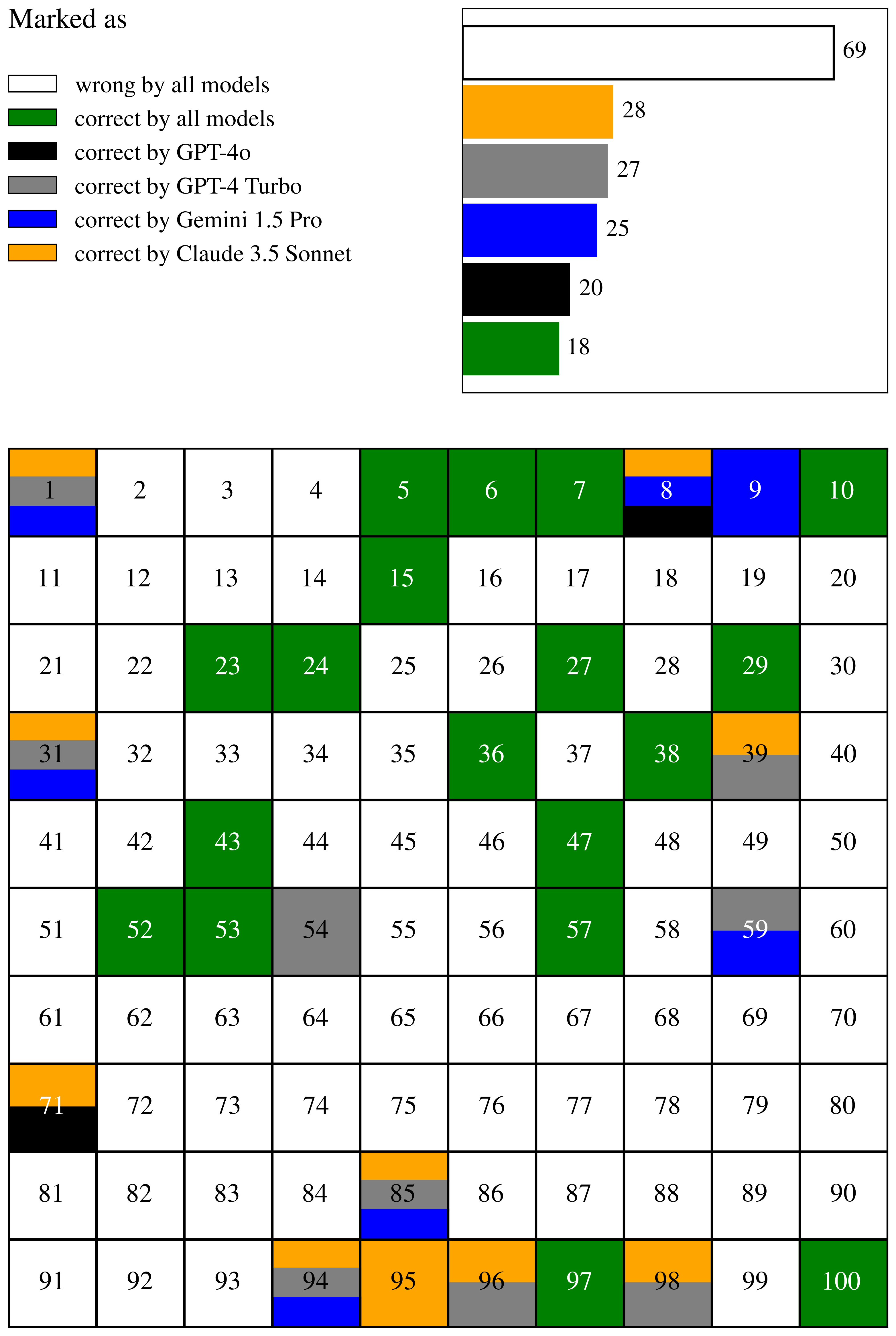
(a) Results with the initial evaluation prompt.

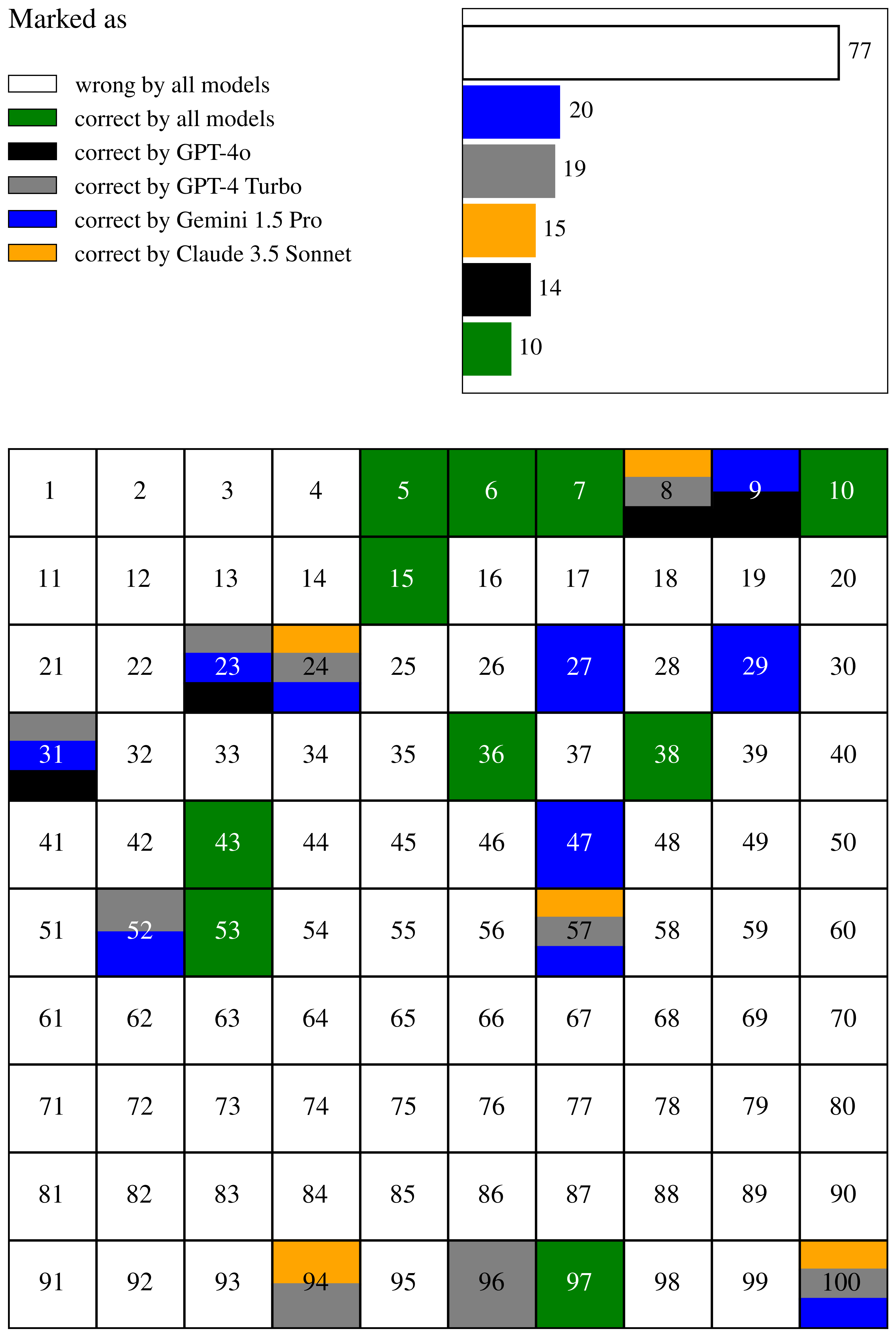
(b) Results with the final evaluation prompt.

Figure 4: Models’ agreement on the evaluation of BPs. The assessed solutions were generated by GPT-4o with the Descriptive strategy. The numbers refer to the BP tasks from (Bongard, 1968). Green indicates tasks unanimously evaluated as correctly solved by all models, while white indicates unanimous incorrect evaluations. Other colors highlight tasks marked as correctly solved by individual models.

B.1 Evaluation prompt optimization

Due to the above evaluation disagreement, we made an attempt to optimize the prompt based on the GPT-4o solutions for the additional $20$ BPs (#101 – #120) that were not used in the main experiments. First, following the few-shot prompting technique, we expanded the prompt to include two examples showing a possible logical difference between correct and incorrect answers. Furthermore, we added a sentence which requested a strict logical compliance with the provided labels. However, this refinement appeared to be too strong, as $2$ (out of $4$) models didn’t evaluate any of the solutions as correct.

To impose some flexibility, we changed the word strictly to logically, but this resulted in an increased rate of false-positive evaluations. Finally, we combined these two prompts, obtaining the outcome closest to the manual (our human) evaluation. The final version of our evaluation prompt is listed in Prompt B.1. Additionally, we attempted to attach the image of the evaluated BP instance to each version of our prompt, but this actually confused the models rather than improving their results, so we ultimately abandoned this option and stuck with the fully text-based prompt.

Although the consistency of results regarded as the number of unanonimous assessments stayed at the same level ($87\%$) (see Fig. 4(b)), the number of answers rated as correct significantly decreased, which was in accordance with our random manual verification.

Despite lowering the results variation, there were still BPs for which the assessment varied. Therefore, we eventually decided to use hard voting to ensemble all models’ evaluations. We marked a solution as correct if at least $2$ of the $4$ models evaluated it as correct. This approach brought better results than the majority voting.

B.2 Manual verification of the evaluation performance of MLLMs

In order to finally assess the efficacy of Prompt B.1 we manually checked the models’ evaluation performance on the $100$ BPs solved by GPT-4o using the Descriptive strategy. As shown in Table 1 in the main paper, all proprietary models achieved better scores on incorrect labels classification. For this reason, we decided to manually verify only the problems evaluated as correct by at least one MLLM, assuming that those incorrect are generally evaluated properly. The comparison between the evaluation performance of the initial and final prompts and our manual evaluation is presented in Table 2. All models denotes evaluations where a solution is marked as correct only if all models evaluate it as correct. Similarly, any model refers to the cases where a solution is marked as correct if at least one model evaluates it as correct. Voting refers to the hard-voting scheme described in section B.1. It is important to observe that the chosen voting evaluation method differed from the manual evaluation in only one specific problem, which is depicted in Fig. 5.

In addition, we checked the performance of our enhanced evaluation prompt on $20$ new, not used in other experiments, manually evaluated Bongard-OpenWorld problems solved by GPT-4o using the Descriptive strategy. Again, the use of Prompt B.1 visibly increased the consensus with manual evaluation (see Table 3). The difference between our manual evaluation and the voting scheme occurred only in 2 problem solutions whose correctness is disputable (see Fig. 6).

Obviously, the choice of examples shown in the prompt may additionally impact the evaluation performance. Nevertheless, the finally proposed evaluation prompt seems to well suit both domains: synthetic and real-world, and should potentially be effective in other similar datasets and solving strategies.

initial prompt			final prompt
All models	Any model	voting	All models	Any model	voting
0.93	0.9	0.94	0.9	0.96	0.99

Table 2: Consensus with manual evaluation on synthetic BPs. The percentage of the solutions evaluated the same as in our manual evaluation in BP instances $\#1-\#100$ (Bongard, 1970). The assessed solutions were obtained by GPT-4o using the Descriptive prompting strategy.

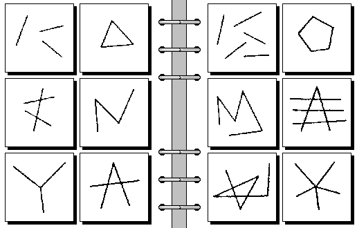
Figure 5: Synthetic BP #85. This is the only BP instance for which the voting-based evaluation of MLLM solutions differed from our manual evaluation. Left: Three parts. Right: Five parts. GPT-4o answer: Left: All images are composed of exactly three lines. Right: All images are composed of more than three lines. Voting marked it as incorrect, whereas in manual evaluation it was marked as correct. The first difference lies in the meaning of the words lines and parts, which, in this visual context, seems identical. The second difference stems from the number of the parts on the right side of the problem. The answer seems to be correct, as obviously, five is more than three. However, one could argue that the answer is incomplete, as each of the squares on the right side clearly depicts exactly five parts.

initial prompt			final prompt
All models	Any model	voting	All models	Any model	voting
0.75	0.7	0.7	0.65	0.85	0.9

Table 3: Consensus with manual evaluation on Bongard-OpenWorld. The percentage of the solutions evaluated the same as in our manual evaluation in the additional 20 Bongard-OpenWorld instances $\#101-\#120$ (Wu et al., 2024), not used in the main experiment. The solutions were obtained by GPT-4o using the Descriptive prompting strategy.

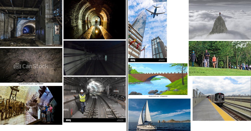
(a) Left: Underground tunnels beneath the city. Right: NOT Underground tunnels beneath the city. GPT-4o solution: Left: All images depict scenes that are primarily indoors or underground. Right: All images depict scenes that are primarily outdoors. We evaluated it as correct, while the voting marked it as incorrect. The difference arises from how the left concept is perceived. Although the images on the left depict an underground setting, they do not appear to represent an indoor scene. Nevertheless, one of the statements is still true.

(b) Left: A woman wearing a white wedding dress. Right: NOT A woman wearing a white wedding dress. GPT-4o solution: Left: All images feature women in white wedding dresses or wedding-related scenes. Right: All images feature women in non-wedding attire, wearing dresses or suits of various colors other than white. We evaluated it as incorrect, while the voting marked it as correct. The difference stems from a small detail in the right concept. One of the images on the right depicts a woman in a white suit, which conflicts with the model’s answer.

Figure 6: The only two Bongard-OpenWorld problems (out of the selected 20) for which the voting evaluation differed from our manual evaluation. The correctness of GPT-4o’s solutions to these problems is disputable.

Appendix C Bongard-RWR dataset

Bongard-RWR dataset developed in this work is attached in the technical appendix and will also be released for the reserach community under the MIT license. The dataset generation algorithm is presented in Algorithm 1 using notation introduced in Section 4.1.

1:A set of synthetic concepts $Y$

2:A set of generated instances ${\cal RWR}$

3:$M\leftarrow 15$,  $N\leftarrow 10$,  $T\leftarrow 3$

4:

5:for $y^{X}\in Y$ do

6:     $D^{X}\leftarrow$ GenerateTranslations($y^{X}$, $N$)

7:     $I^{X}\leftarrow\emptyset$,  $P\leftarrow\emptyset$

8:

9:     for $D^{X}_{i}\in D^{X}$ do

10:         for $m\leftarrow 1$ to $M$ do

11:              for $S\in\{L,R\}$ do

12:                  $I\leftarrow$ DownloadImage($D^{XS}_{i}$, $m$)

13:                  if $I$ is accepted by model then

14:                       $I^{XS}_{i}\leftarrow I^{XS}_{i}\cup\{I\}$

15:                  end if

16:              end for

17:

18:              if $|I^{XL}_{i}|\geq 2$ and $|I^{XR}_{i}|\geq 2$ then

19:                  $P\leftarrow P\cup\{i\}$

20:                  break

21:              end if

22:         end for

23:

24:         if $|P|\geq T$ then

25:              Break

26:         end if

27:     end for

28:

29:     ${\cal L}^{X}\leftarrow\emptyset$,  ${\cal R}^{X}\leftarrow\emptyset$

30:     if $|P|\geq T$ then

31:         for $k\leftarrow 1$ to $6$ do

32:              $p\leftarrow P[k\mod T]$

33:              $j\leftarrow k\div T$

34:              for $S\in\{L,R\}$ do

35:                  ${\cal S}^{X}\leftarrow{\cal S}^{X}\cup\{I^{XS}_{p}(j)\}$

36:              end for

37:         end for

38:

39:         ${\cal RWR}^{X}\leftarrow\{{\cal L}^{X},{\cal R}^{X}\}$

40:         ${\cal RWR}\leftarrow{\cal RWR}\cup\{{\cal RWR}^{X}\}$

41:     end if

42:end for

Algorithm 1 The Bongard-RWR dataset generation.

Furthermore, Fig. 8 provides additional examples of the proposed Bongard-RWR dataset. Each subfigure presents a comparison between the synthetic Bongard problem and its respective real-world translation in Bongard-RWR. Examples 8(a) and 8(b) were translated automatically, whereas 8(c) and 8(d) were constructed fully manually, including building an appropriate scene and taking a picture. Additionally, Fig. 7 shows a particular approach taken when translating a given synthetic BP to its Bongard-RWR counterpart (problems not translated and those rejected after translation are combined into one category).

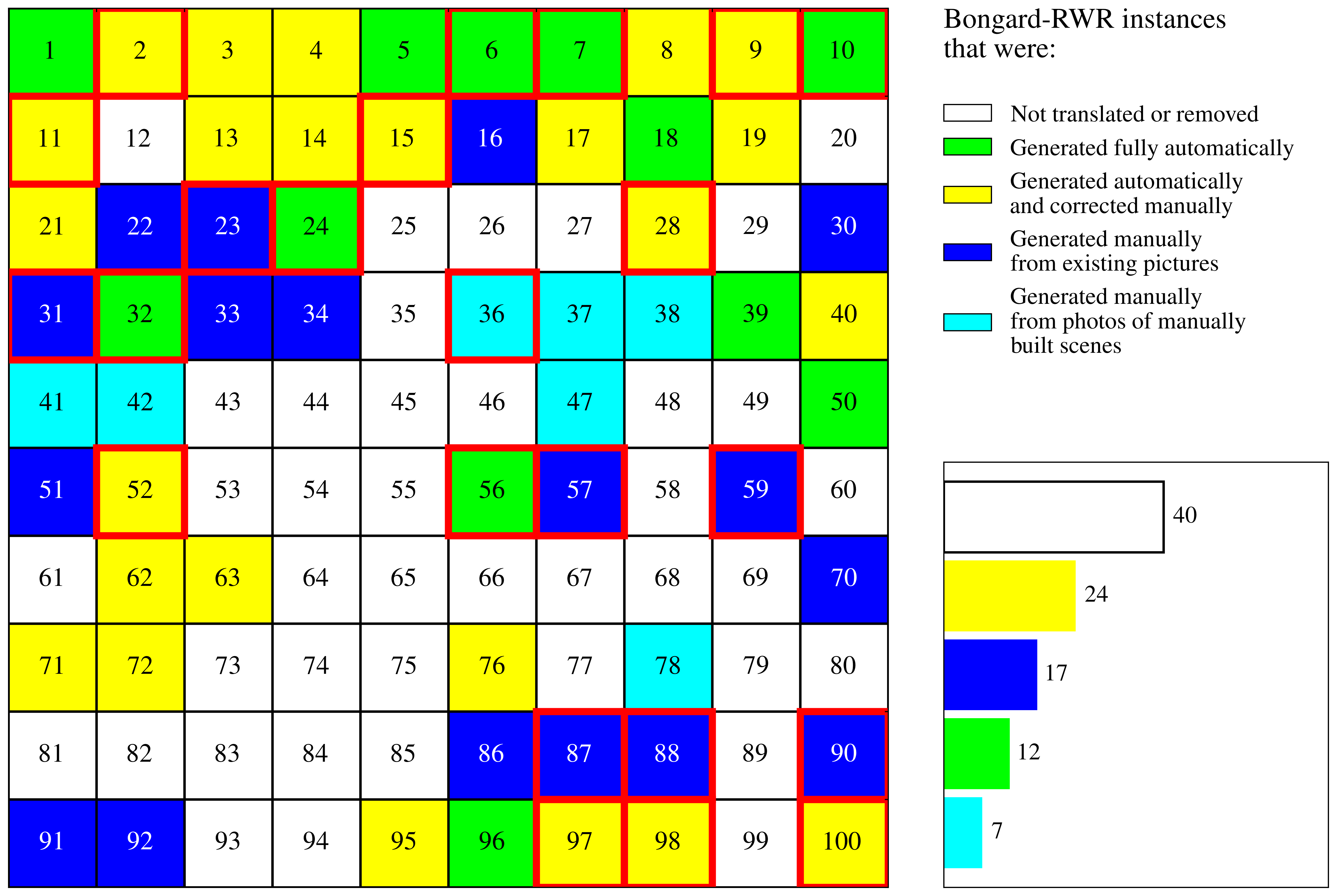
Figure 7: The structure of the Bongard-RWR dataset. Each color denotes the genesis of the translation of the respective problem. Problems not translated and those rejected after translation are combined into one category. Red color outlines denote problems which were solved by any model using any strategy. There is no visible correlation between the set of solved problem and the methods used for their generation.

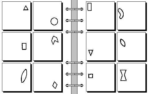
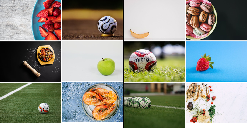
(a) Synthetic BP #8 with its automatically translated Bongard-RWR version. Left: Ends of the curve are far apart. Right: Ends of the curve are close together.

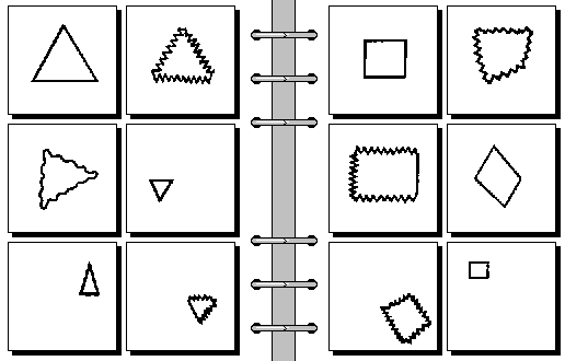
(b) Synthetic BP #10 with its automatically translated Bongard-RWR version. Left: Triangles. Right: Quadrangles.

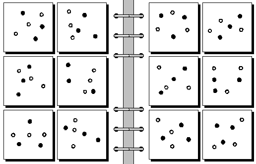
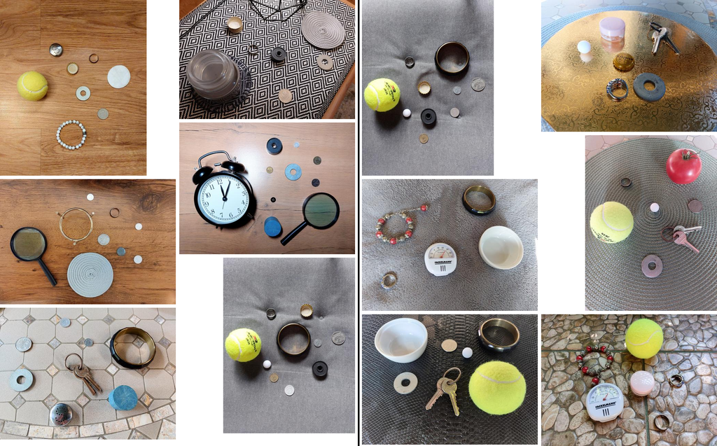
(c) Synthetic BP #41 with it manually constructed Bongard-RWR version. Left: Outline circles on one straight line. Right: Outline circles not on one straight line.

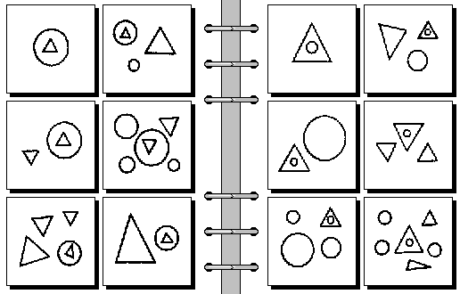
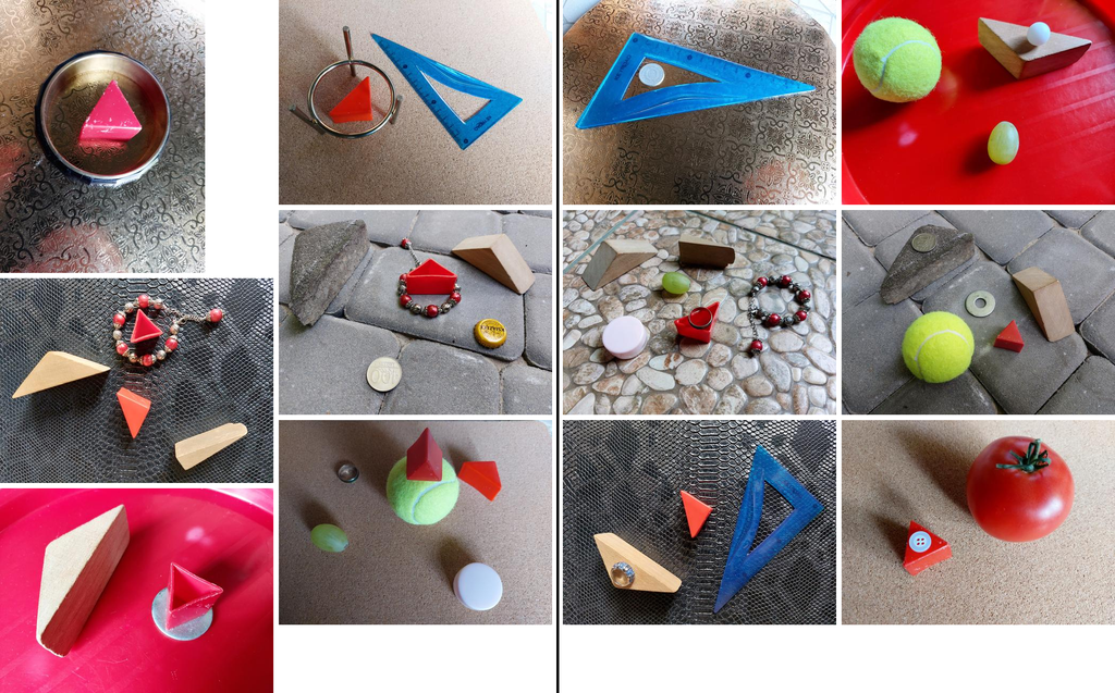
(d) Synthetic BP #47 with its manually constructed Bongard-RWR version. Left: Triangle on top of the circle. Right: Circle on top of the triangle.

Figure 8: Additional examples of Bongard-RWR instances.

Appendix D Coverage of Bongard-RWR instances

Even though the final results of individual models and strategies solving Bongard-RWR are somewhat unsatisfactory, especially in the case of open language response generation, it is worth to examine the degree of overlap of correct answers across the tested models. On the one hand, the results of ground-truth classification and model’s disagreement on the solution evaluation clearly confirm inability of any single model to solving all problems from the Bongard-RWR datatset. On the other hand, it is likely that the overlap is not complete, and it is posible to expand the solution coverage by appropriate mixture-of-experts approach. This is indeed the case in our experiments, as illustrated in Figures 9 - 16. While single proprietary MLLMs solved between $9$ and $14$ instances, the number of instances solved by any MLLM equaled $23$. We leave exploration of this path for future research.

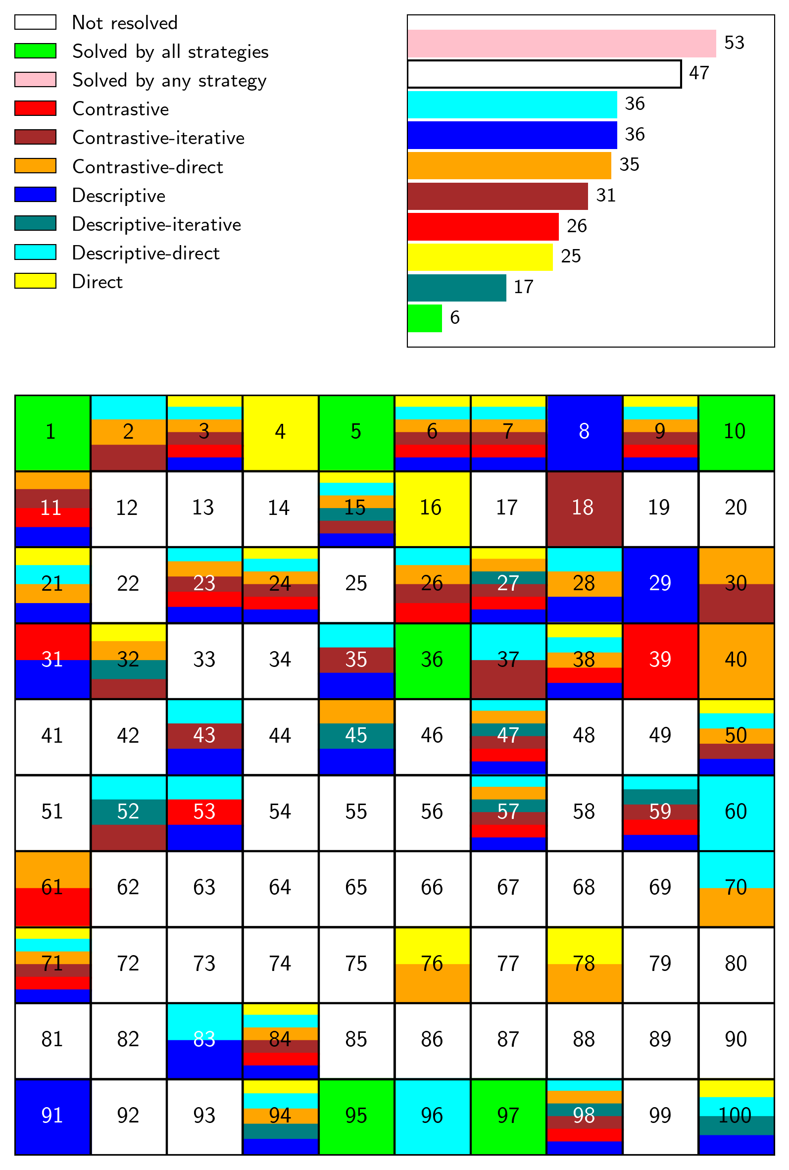
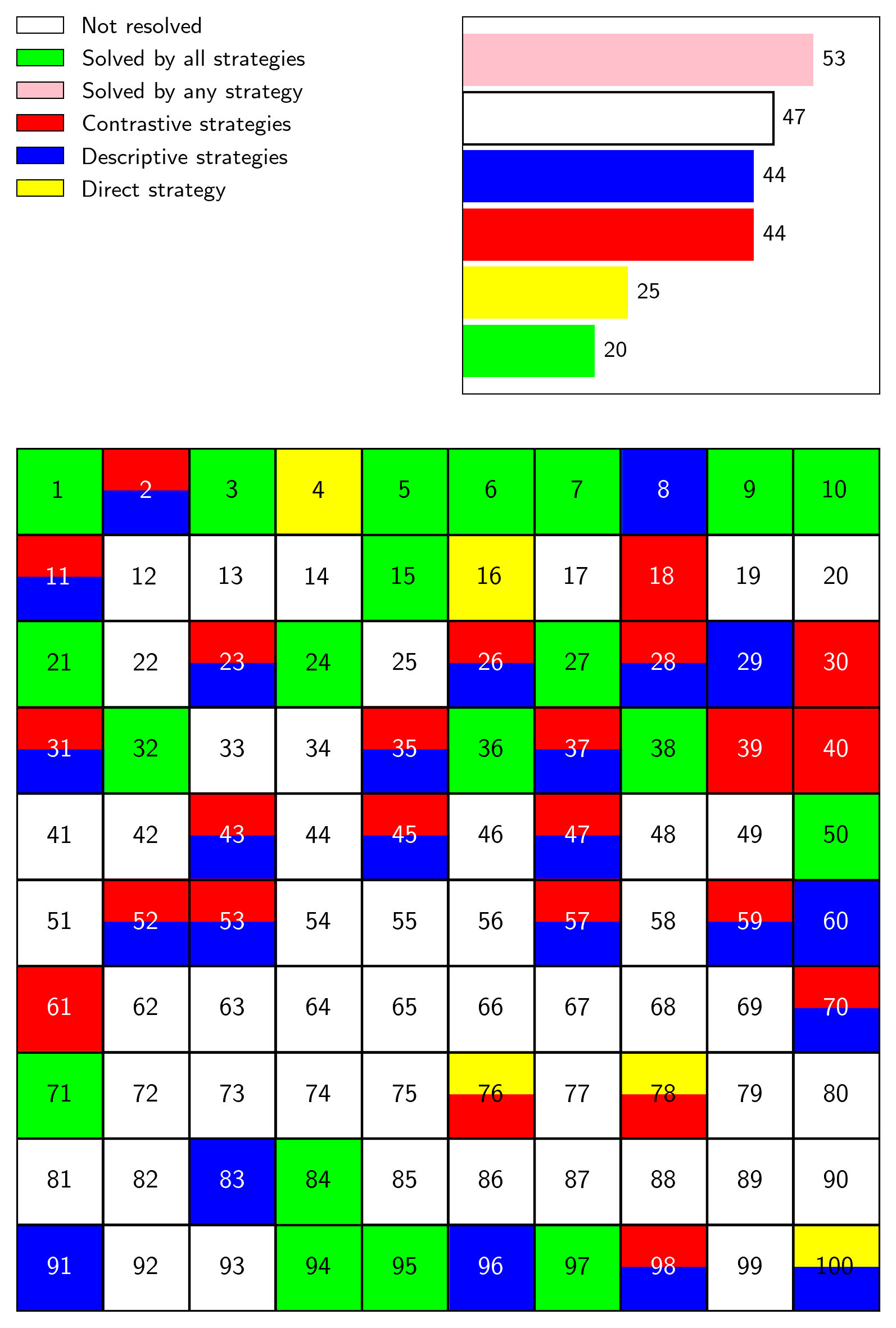
Figure 9: Overall result of each strategy on synthethic BPs. Colormaps depict all problems solved by any tested model using the respective prompting strategy. The right figure aggregates strategies into corresponding groups for better coverage exposure.

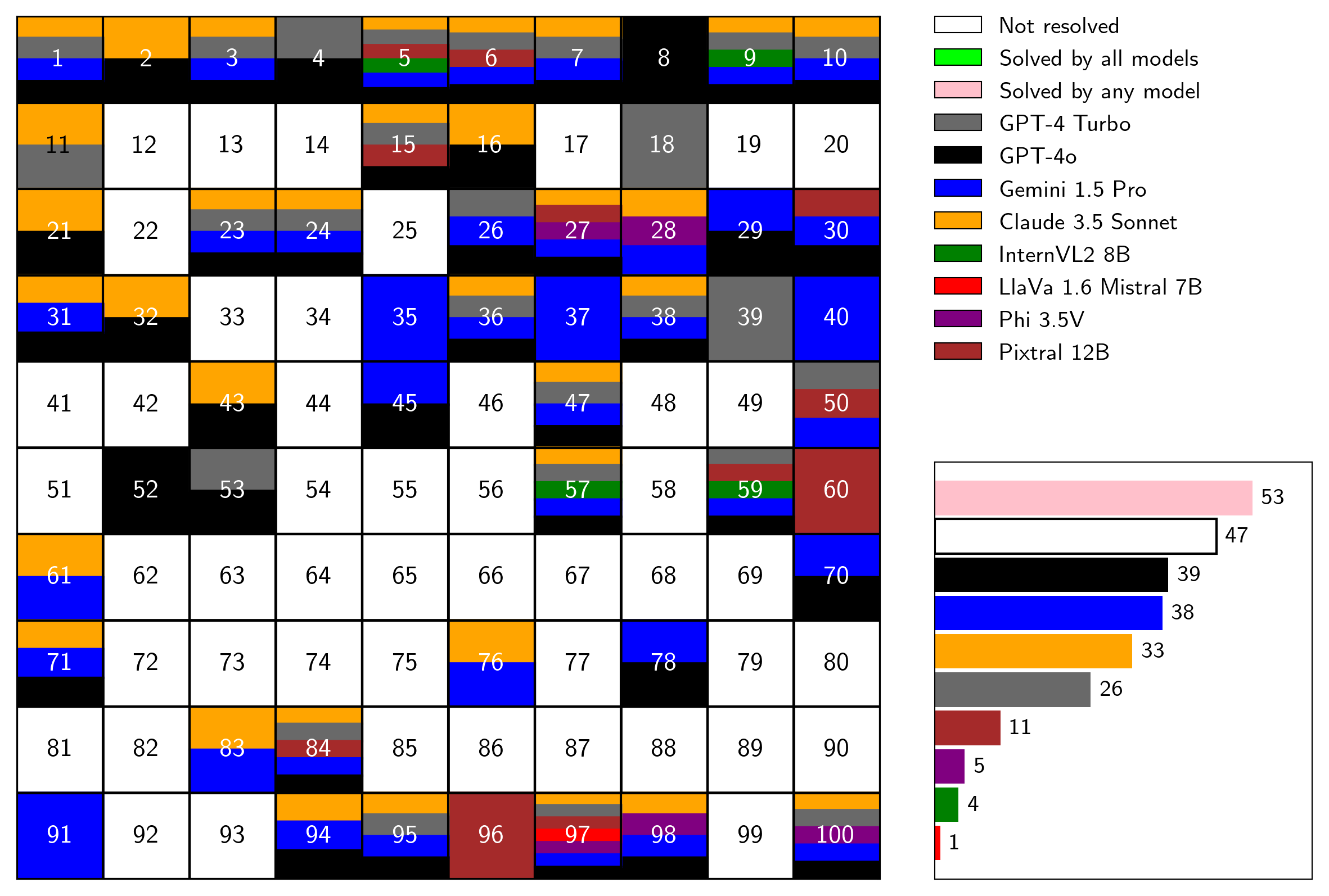
Figure 10: Final summary of all experiments on the synthetic Bongard Problems dataset. The colormap aggregates all problems solved by any tested model using any generation prompting strategy. Overall, the models collectively managed to solve 53 problems.

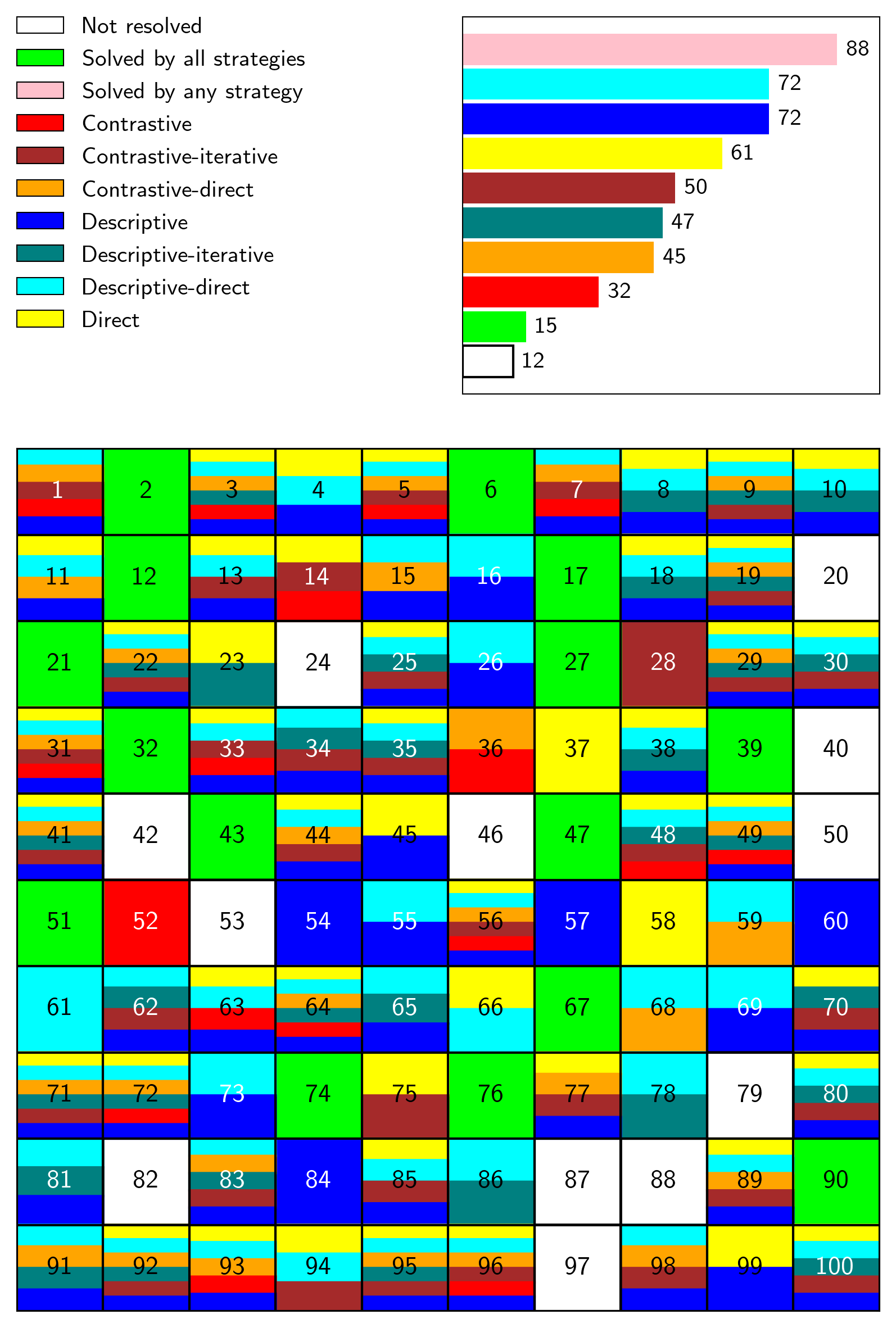
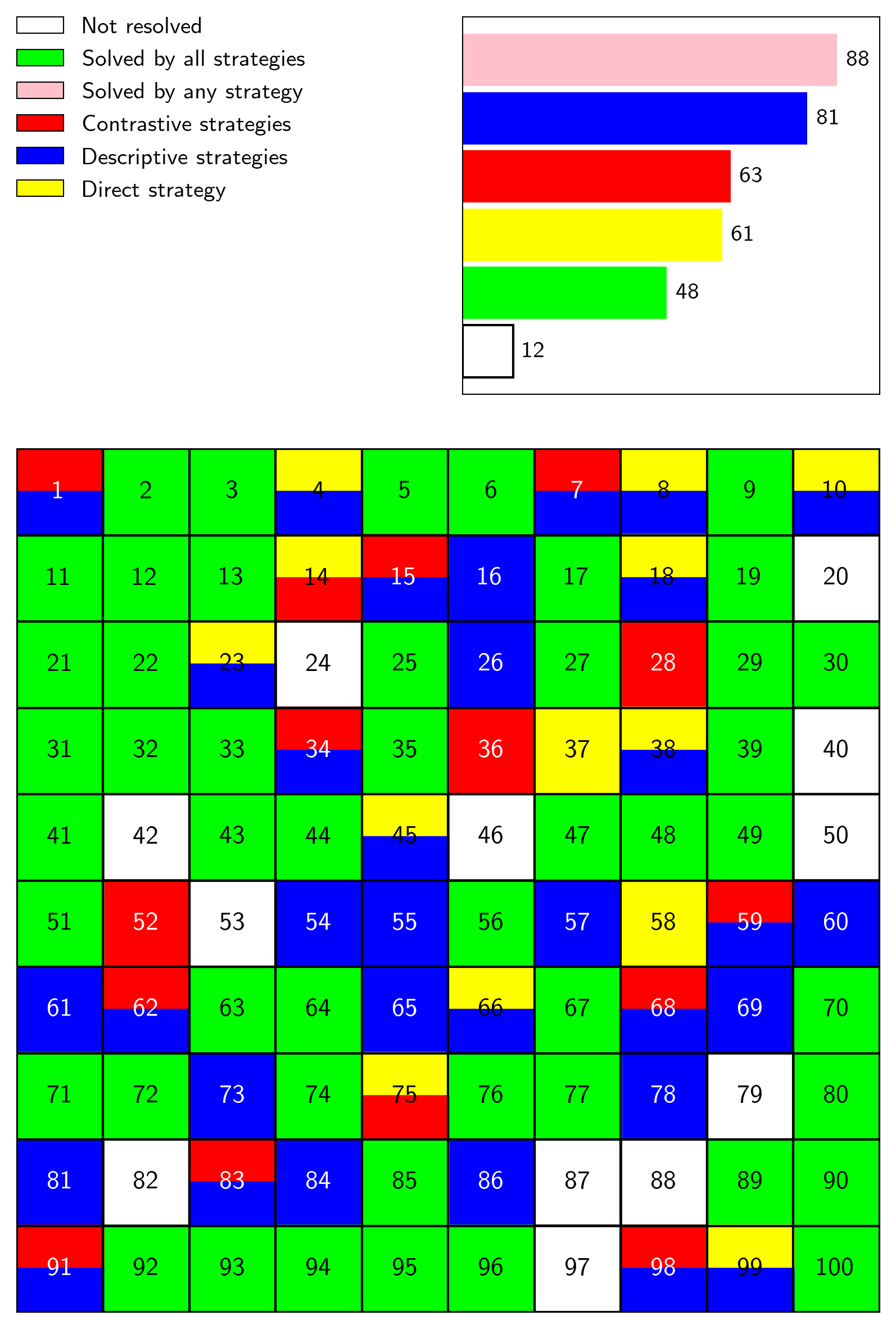
Figure 11: Overall result of each strategy on Bongard HOI. Colormaps depict all problems solved by any tested model using the respective prompting strategy. The right figure aggregates strategies into corresponding groups for better coverage exposure.

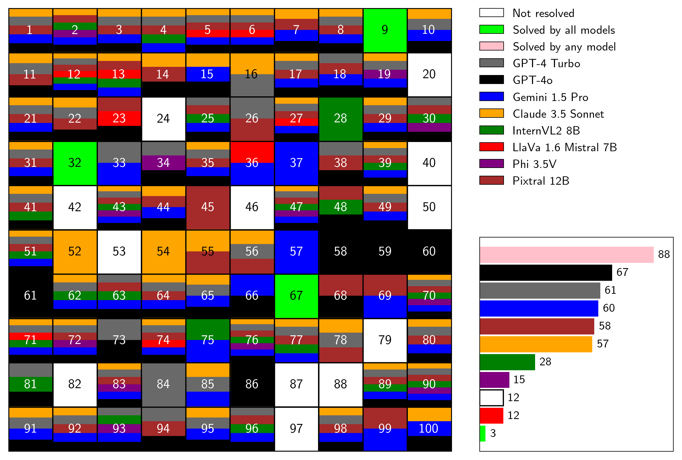
Figure 12: Final summary of all experiments on the Bongard HOI dataset. The colormap aggregates all problems solved by any tested model using any generation prompting strategy. Overall, the models collectively managed to solve 88 problems.

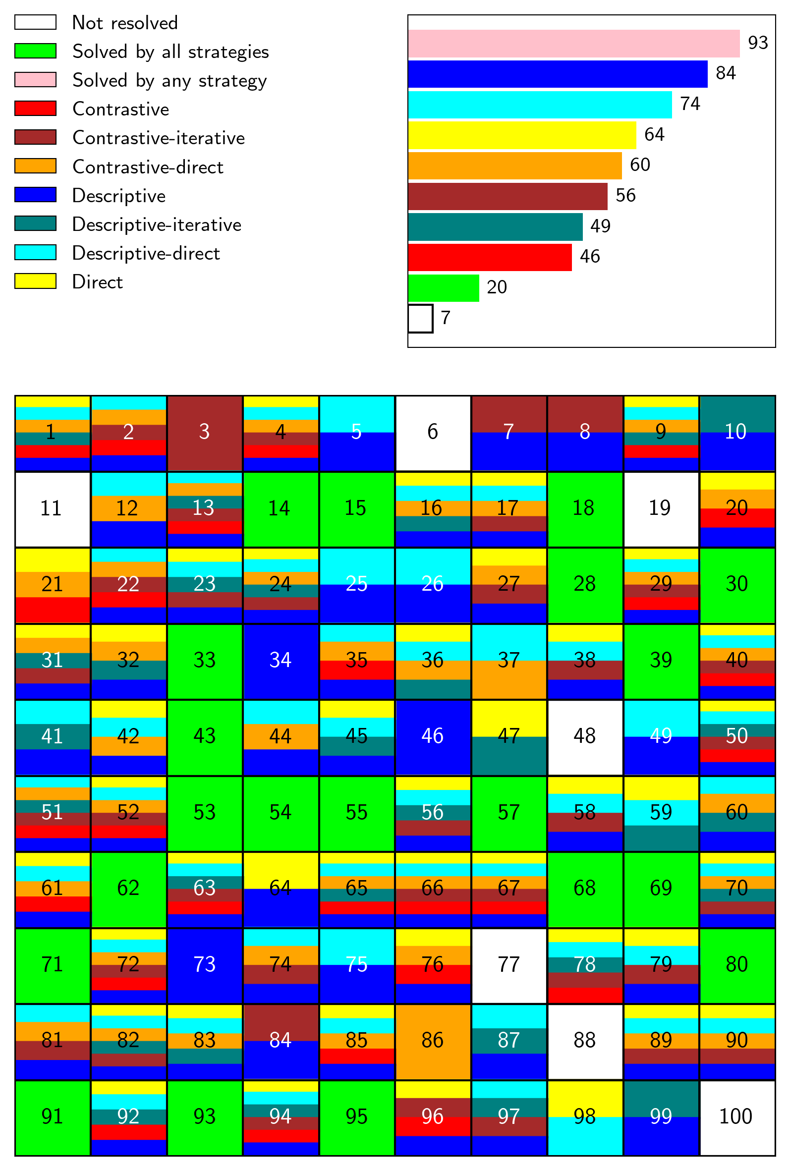
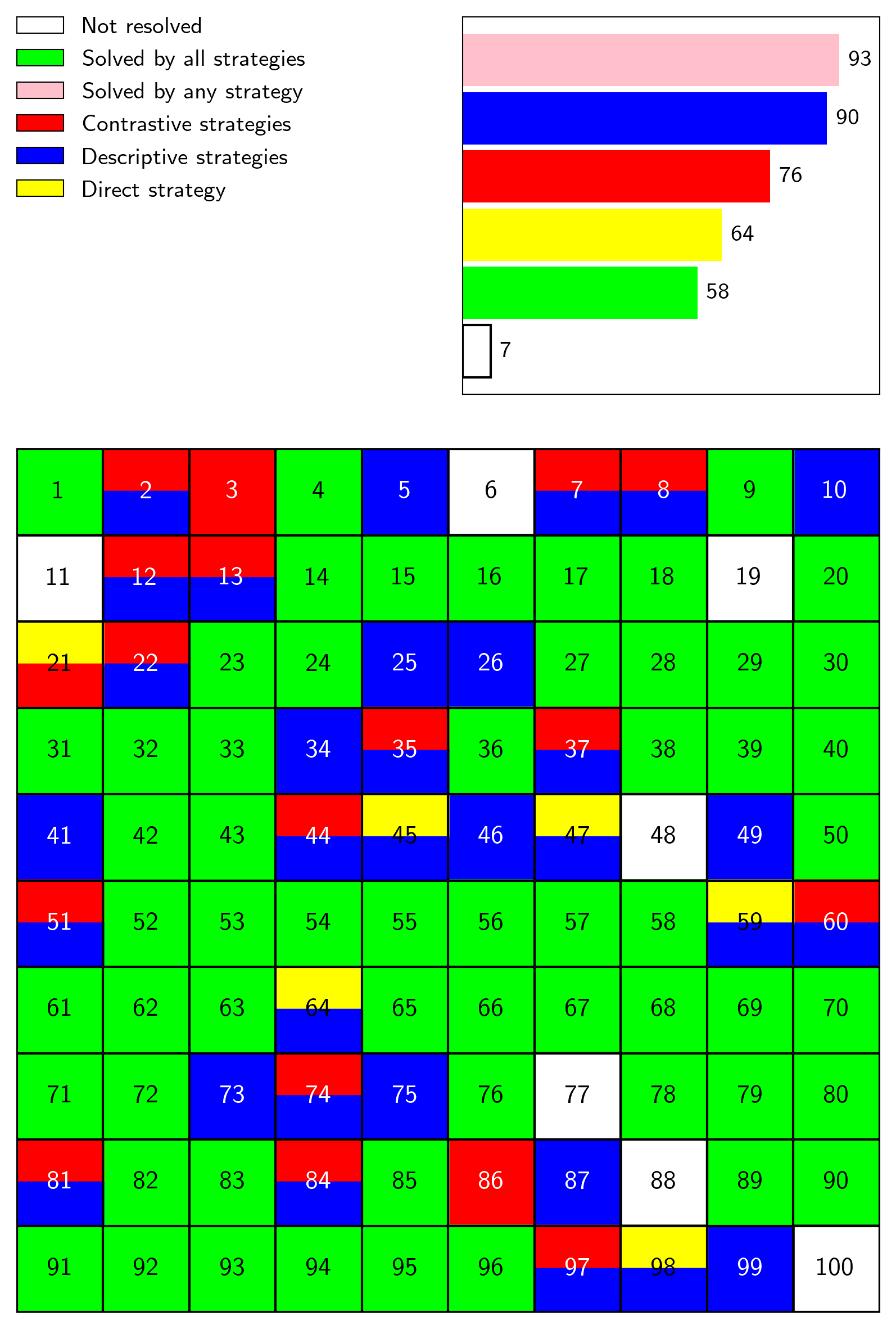
Figure 13: Overall result of each strategy on Bongard-OpenWorld. Colormaps depict all problems solved by any tested model using the respective prompting strategy. The right figure aggregates strategies into corresponding groups for better coverage exposure.

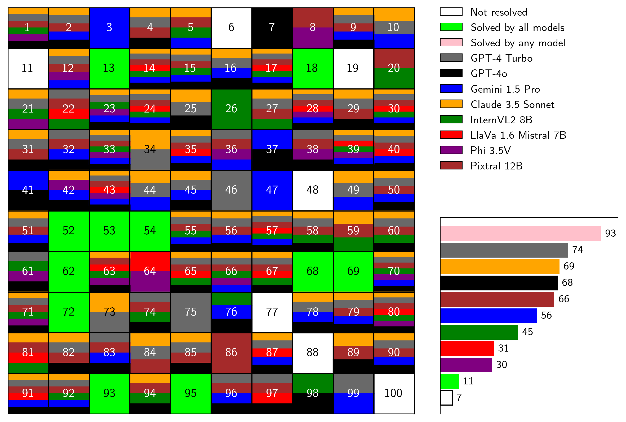
Figure 14: Final summary of all experiments on the Bongard-OpenWorld dataset. The colormap aggregates all problems solved by any tested model using any generation prompting strategy. Overall, the models collectively managed to solve 93 problems.

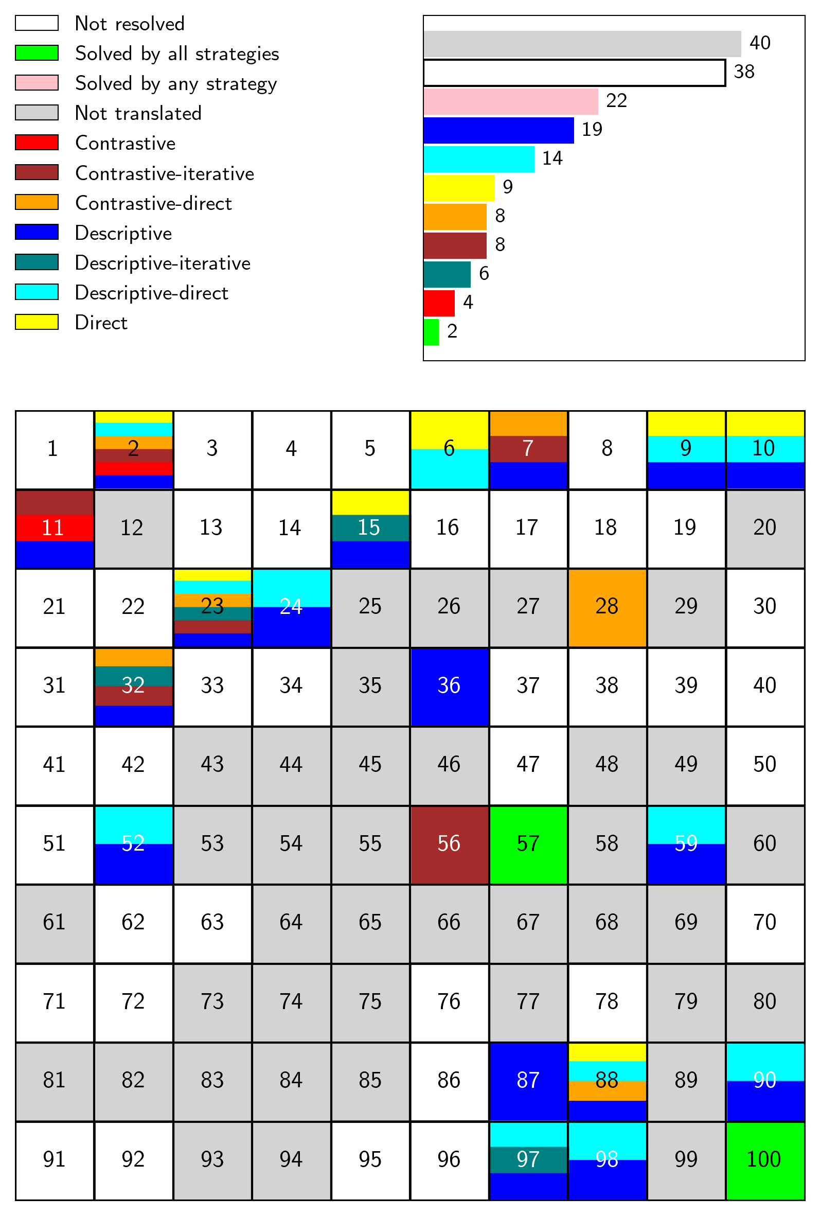
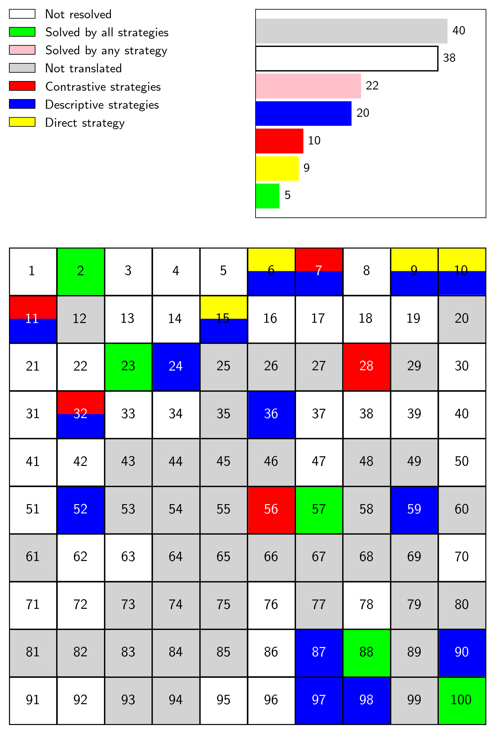
Figure 15: Overall result of each strategy on Bongard-RWR. Colormaps depict all problems solved by any tested model using the respective prompting strategy. The right figure aggregates strategies into corresponding groups for better coverage exposure.

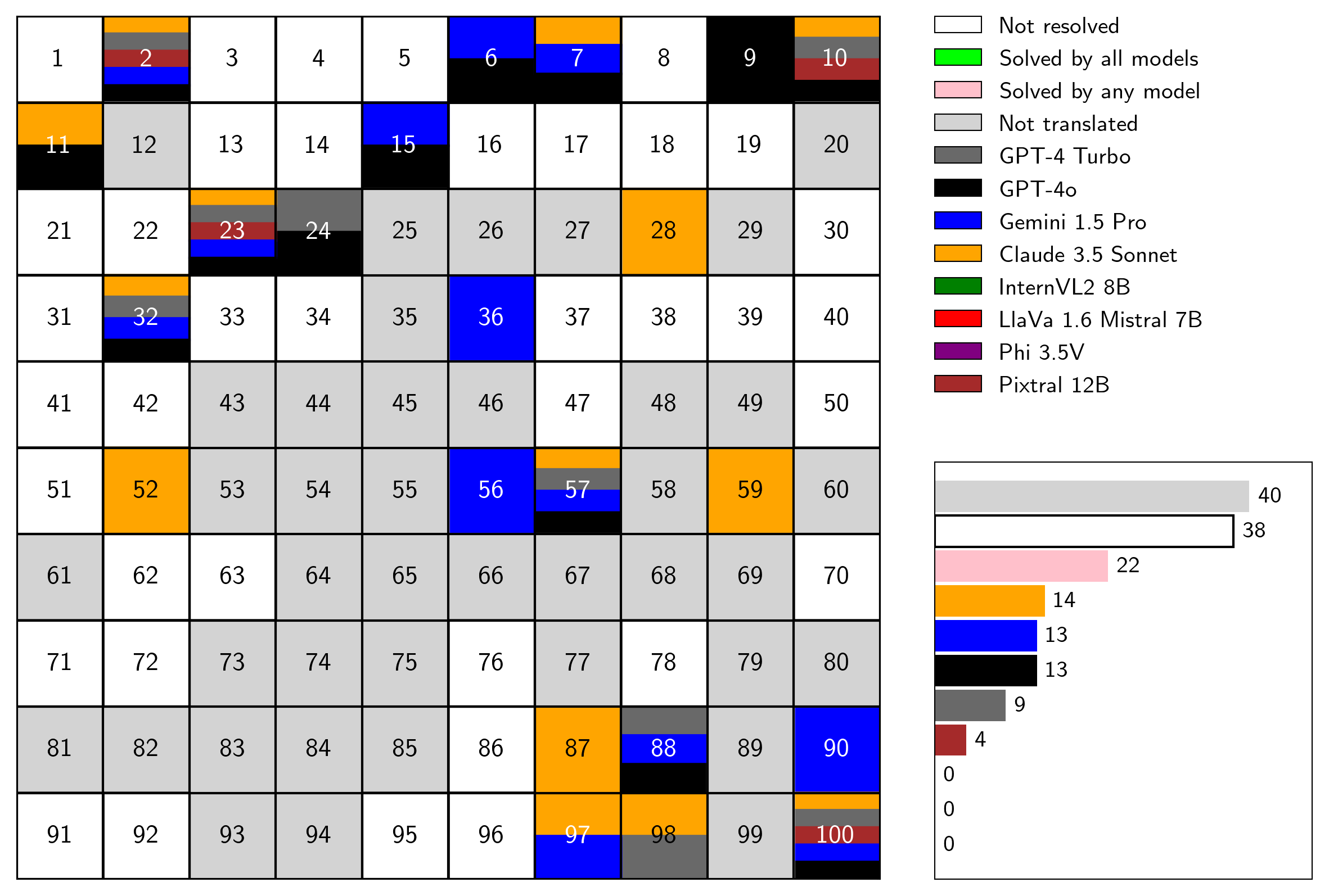
Figure 16: Final summary of all experiments on the Bongard-RWR dataset. The colormap aggregates all problems solved by any tested model using any generation prompting strategy. Overall, the models collectively managed to solve 23 problems.

Appendix E Comparison of Synthetic Bongard vs. Bongard-RWR Results

Our research shows that all of the tested models have difficulty solving synthetic concepts when applied to real-world images. Comparing the results for both datasets (see Figures 10 and 16) we identified some discrepancies. Four problems that remained unsolved in the synthetic BPs were successfully solved in the real-world domain of the Bongard-RWR dataset: #56, #87, #88, and #98. However, three of these problems differ slightly from their synthetic counterparts. The images in #56 from Bongard-RWR feature a variety of colors instead of the usual black-and-white figures. Furthermore, in real-world version of problem #87 more images feature disjoint elements instead of multi-part objects, which may have nudged the model toward the correct answer. Additionally, in problem #98, the figures are shown against a hatched texture, which was not accounted for in the real-world translation.

Conversely, 22 problems that were solved in the synthetic BPs were not solved in the Bongard-RWR dataset. In most cases, the models focused on general associations that did not apply to all the images. For example, the concept presented in problem #3 is: ”LEFT: Outline figures, RIGHT: Solid figures.” Claude 3.5 Sonnet, using the Descriptive strategy, responded: ”LEFT: focuses on practical, everyday objects or scenes, RIGHT: emphasizes aesthetic, artistic, or decorative elements that serve more for visual appeal than utility”. Nevertheless, both sides feature a red coffee cup with a saucer, which matches both generated descriptions. The key difference lies in the color of the saucer’s rim, which determines whether it should be considered as an outline or a solid figure.

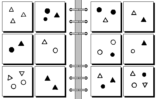
(a) Model’s answer: ”Left: All shapes are filled. Right: At least one shape is unfilled”. Evaluated as incorrect.

(b) Model’s answer: ”Left: Images are monochromatic (containing only shades of a single color). Right: All images contain at least one hollow (unfilled) shape”. Evaluated as correct.

Figure 17: Synthetic BP #56 with its automatically translated Bongard-RWR version. Correct answer: ”Left: All figures of the same color. Right: Figures of different colors”. Provided answers belong to Gemini 1.5 Pro using the Contrastive-iterative strategy, as it was the only combination that solved this Bongard-RWR instance correctly.

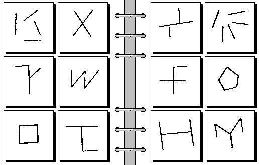
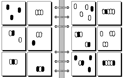
(a) Model’s answer: ”Left: All shapes are composed of straight lines that form only acute or right angles. Right: All shapes contain at least one instance of obtuse angles or curves (e.g., pentagon, ”H” shape, radial pattern)”. Evaluated as incorrect.

(b) Model’s answer: ”Left: All images contain exactly four of something: four orange slices, Four cake slices, four lobes of the four-leaf clover, four pineapples, four fingers with painted nails (thumb not visible), four visible elements (key, keychain, watch/compass, leather strap). Right: Images do not contain exactly four of any element: single four-leaf clover, multiple keys on a ring, single street lamp with multiple lights, single ladybug, multiple oranges (more than four), stack of five cookies”. Evaluated as correct.

Figure 18: Synthetic BP #87 with its manually translated Bongard-RWR version. Correct answer: ”Left: Four parts. Right: Five parts”. Provided answers belong to Claude 3.5 Sonnet using the Descriptive strategy, as it was the only combination that solved this Bongard-RWR instance correctly.

(a) Model’s answer: ”Left: Each image contains an even number of shapes. Right: Each image contains an odd number of shapes”. Evaluated as incorrect.

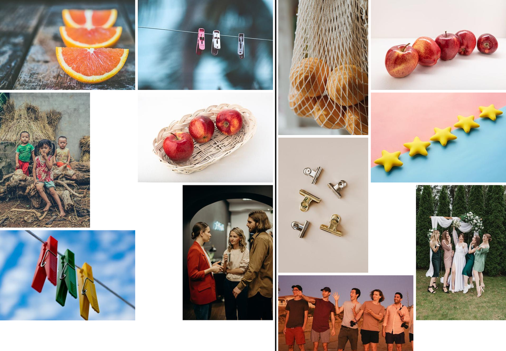
(b) Model’s answer: ”Left: Contains groups of three items. Right: Contains groups of five items”. Evaluated as correct.

Figure 19: Synthetic BP #88 with its manually translated Bongard-RWR version. Correct answer: ”Left: Three parts. Right: Five parts”. Provided answers belong to GPT-4o using the Direct strategy. Overall this problem was solved by three models and four strategies.

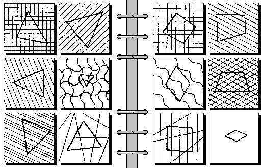
(a) Model’s answer: ”Left: All images contain geometric shapes or patterns that are oriented or have components that predominantly point to the right. Right: All images contain geometric shapes or patterns that are either static (not pointing in any specific direction) or have components that do not predominantly point to the right”. Evaluated as incorrect.

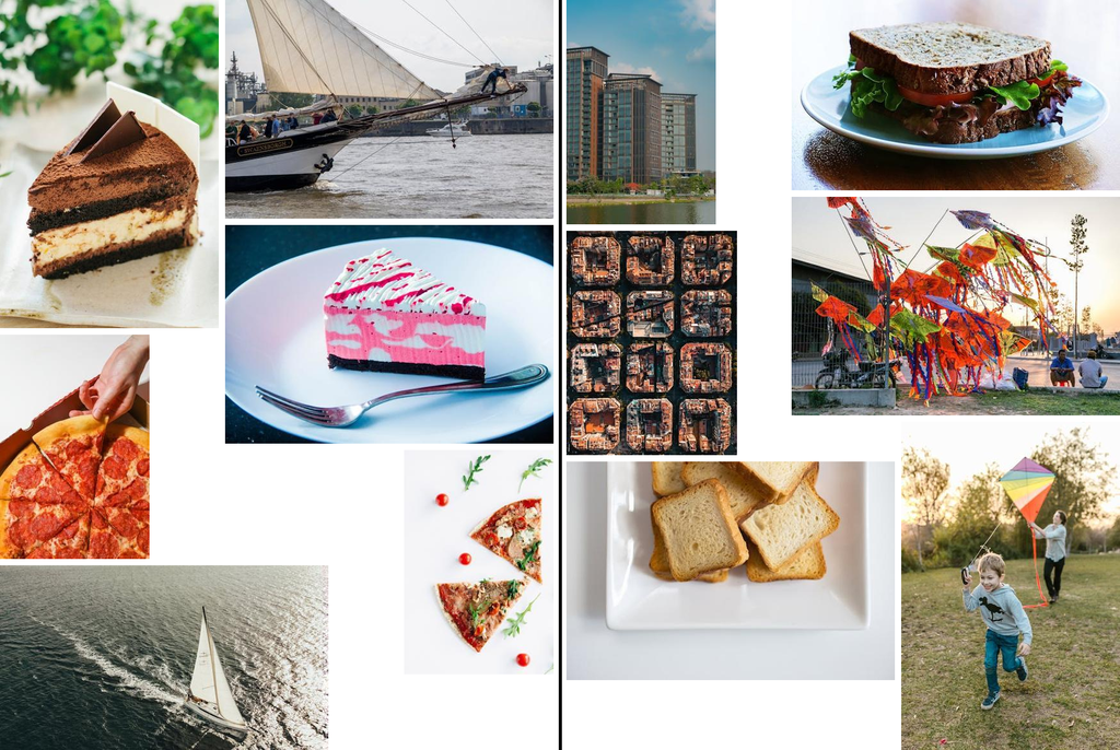
(b) Model’s answer: ”Left: All images on the left side feature objects that are primarily triangular in shape. This includes the slices of cake and pizza, which are cut into triangular pieces, and the sailboats, which have triangular sails. Right: All images on the right side feature objects or scenes that are primarily rectangular or square in shape. This includes the modern buildings, the sandwich, the grid-like urban area, the arrangement of kites, and the plate of toasted bread, all of which emphasize rectangular or square forms”. Evaluated as correct.

Figure 20: Synthetic BP #98 with its manually corrected Bongard-RWR version. Correct answer: ”Left: Three parts. Right: Five parts”. Provided answers belong to GPT-4 Turbo using the Descriptive-direct strategy. Overall this problem was solved by two models using two different strategies.

References

- Abdin et al. (2024) Marah Abdin, Sam Ade Jacobs, Ammar Ahmad Awan, Jyoti Aneja, Ahmed Awadallah, Hany Awadalla, Nguyen Bach, Amit Bahree, Arash Bakhtiari, Harkirat Behl, et al. Phi-3 technical report: A highly capable language model locally on your phone. arXiv preprint arXiv:2404.14219, 2024.
- Achiam et al. (2023) Josh Achiam, Steven Adler, Sandhini Agarwal, Lama Ahmad, Ilge Akkaya, Florencia Leoni Aleman, Diogo Almeida, Janko Altenschmidt, Sam Altman, Shyamal Anadkat, et al. Gpt-4 technical report. arXiv preprint arXiv:2303.08774, 2023.
- Anthropic (2024) Anthropic. The claude 3 model family: Opus, sonnet, haiku. 2024.
- Barrett et al. (2018) David Barrett, Felix Hill, Adam Santoro, Ari Morcos, and Timothy Lillicrap. Measuring abstract reasoning in neural networks. In International Conference on Machine Learning, pp. 511–520. PMLR, 2018.
- Bitton et al. (2023) Yonatan Bitton, Ron Yosef, Eliyahu Strugo, Dafna Shahaf, Roy Schwartz, and Gabriel Stanovsky. Vasr: Visual analogies of situation recognition. In Proceedings of the AAAI Conference on Artificial Intelligence, volume 37, pp. 241–249, 2023.
- Bongard (1968) Mikhail Moiseevich Bongard. The recognition problem. Technical report, Foreign Technology Div Wright-Patterson AFB Ohio, 1968.
- Bongard (1970) Mikhail Moiseevich Bongard. Pattern Recognition. Spartan Books, 1970.
- Brown et al. (2020) Tom Brown, Benjamin Mann, Nick Ryder, Melanie Subbiah, Jared D Kaplan, Prafulla Dhariwal, Arvind Neelakantan, Pranav Shyam, Girish Sastry, Amanda Askell, et al. Language models are few-shot learners. Advances in neural information processing systems, 33:1877–1901, 2020.
- Camposampiero et al. (2023) Giacomo Camposampiero, Loïc Houmard, Benjamin Estermann, Joël Mathys, and Roger Wattenhofer. Abstract visual reasoning enabled by language. In Proceedings of the IEEE/CVF Conference on Computer Vision and Pattern Recognition, pp. 2643–2647, 2023.
- Cao et al. (2024) Xu Cao, Bolin Lai, Wenqian Ye, Yunsheng Ma, Joerg Heintz, Jintai Chen, Jianguo Cao, and James M Rehg. What is the visual cognition gap between humans and multimodal llms? arXiv preprint arXiv:2406.10424, 2024.
- Carbonell (1983) Jaime G Carbonell. Learning by analogy: Formulating and generalizing plans from past experience. In Machine learning, pp. 137–161. Elsevier, 1983.
- Chalmers et al. (1992) David J Chalmers, Robert M French, and Douglas R Hofstadter. High-level perception, representation, and analogy: A critique of artificial intelligence methodology. Journal of Experimental & Theoretical Artificial Intelligence, 4(3):185–211, 1992.
- Chen et al. (2021) Yinbo Chen, Zhuang Liu, Huijuan Xu, Trevor Darrell, and Xiaolong Wang. Meta-baseline: Exploring simple meta-learning for few-shot learning. In Proceedings of the IEEE/CVF international conference on computer vision, pp. 9062–9071, 2021.
- Chen et al. (2024a) Zhe Chen, Weiyun Wang, Hao Tian, Shenglong Ye, Zhangwei Gao, Erfei Cui, Wenwen Tong, Kongzhi Hu, Jiapeng Luo, Zheng Ma, et al. How far are we to gpt-4v? closing the gap to commercial multimodal models with open-source suites. arXiv preprint arXiv:2404.16821, 2024a.
- Chen et al. (2024b) Zhe Chen, Jiannan Wu, Wenhai Wang, Weijie Su, Guo Chen, Sen Xing, Muyan Zhong, Qinglong Zhang, Xizhou Zhu, Lewei Lu, et al. Internvl: Scaling up vision foundation models and aligning for generic visual-linguistic tasks. In Proceedings of the IEEE/CVF Conference on Computer Vision and Pattern Recognition, pp. 24185–24198, 2024b.
- Chollet (2019) François Chollet. On the measure of intelligence. arXiv preprint arXiv:1911.01547, 2019.
- Depeweg et al. (2018) Stefan Depeweg, Constantin A Rothkopf, and Frank Jäkel. Solving bongard problems with a visual language and pragmatic reasoning. arXiv preprint arXiv:1804.04452, 2018.
- Depeweg et al. (2024) Stefan Depeweg, Contantin A Rothkopf, and Frank Jäkel. Solving bongard problems with a visual language and pragmatic constraints. Cognitive Science, 48(5):e13432, 2024.
- Falkenhainer et al. (1989) Brian Falkenhainer, Kenneth D Forbus, and Dedre Gentner. The structure-mapping engine: Algorithm and examples. Artificial intelligence, 41(1):1–63, 1989.
- Fei-Fei et al. (2006) Li Fei-Fei, Robert Fergus, and Pietro Perona. One-shot learning of object categories. IEEE transactions on pattern analysis and machine intelligence, 28(4):594–611, 2006.
- Fleuret et al. (2011) François Fleuret, Ting Li, Charles Dubout, Emma K Wampler, Steven Yantis, and Donald Geman. Comparing machines and humans on a visual categorization test. Proceedings of the National Academy of Sciences, 108(43):17621–17625, 2011.
- Foundalis (2006a) Harry E Foundalis. Phaeaco: A cognitive architecture inspired by Bongard’s problems. PhD dissertation, Indiana University, 2006a.
- Foundalis (2006b) Harry E Foundalis. Index of bongard problems. http://www.foundalis.com/res/bps/bpidx.htm, 2006b. Accessed: 2024-08-01.
- Gardner & Richards (2006) Martin Gardner and Dana Richards. The colossal book of short puzzles and problems. Norton, 2006.
- Gentner (1983) Dedre Gentner. Structure-mapping: A theoretical framework for analogy. Cognitive science, 7(2):155–170, 1983.
- Hill et al. (2019) Felix Hill, Adam Santoro, David Barrett, Ari Morcos, and Timothy Lillicrap. Learning to Make Analogies by Contrasting Abstract Relational Structure. In International Conference on Learning Representations (ICLR), 2019.
- Hofstadter (1995) Douglas R Hofstadter. Fluid concepts and creative analogies: Computer models of the fundamental mechanisms of thought. Basic books, 1995.
- Hofstadter (1999) Douglas R Hofstadter. Gödel, Escher, Bach: an eternal golden braid. Basic books, 1999.
- Holyoak & Thagard (1989) Keith J Holyoak and Paul Thagard. Analogical mapping by constraint satisfaction. Cognitive science, 13(3):295–355, 1989.
- Ichien et al. (2021) Nicholas Ichien, Qing Liu, Shuhao Fu, Keith J Holyoak, Alan Yuille, and Hongjing Lu. Visual analogy: Deep learning versus compositional models. arXiv preprint arXiv:2105.07065, 2021.
- Jiang et al. (2023) AQ Jiang, A Sablayrolles, A Mensch, C Bamford, DS Chaplot, D de las Casas, F Bressand, G Lengyel, G Lample, L Saulnier, et al. Mistral 7b (2023). arXiv preprint arXiv:2310.06825, 2023.
- Jiang et al. (2022) Huaizu Jiang, Xiaojian Ma, Weili Nie, Zhiding Yu, Yuke Zhu, and Anima Anandkumar. Bongard-hoi: Benchmarking few-shot visual reasoning for human-object interactions. In Proceedings of the IEEE/CVF conference on computer vision and pattern recognition, pp. 19056–19065, 2022.
- Jiang et al. (2024) Yifan Jiang, Jiarui Zhang, Kexuan Sun, Zhivar Sourati, Kian Ahrabian, Kaixin Ma, Filip Ilievski, and Jay Pujara. Marvel: Multidimensional abstraction and reasoning through visual evaluation and learning. arXiv preprint arXiv:2404.13591, 2024.
- Kharagorgiev (2018) Sergii Kharagorgiev. Solving bongard problems with deep learning. https://k10v.github.io/2018/02/25/Solving-Bongard-problems-with-deep-learning/, February 2018. Accessed: 2024-08-01.
- Lake et al. (2017) Brenden M Lake, Tomer D Ullman, Joshua B Tenenbaum, and Samuel J Gershman. Building machines that learn and think like people. Behavioral and brain sciences, 40:e253, 2017.
- Lee et al. (2019) Kwonjoon Lee, Subhransu Maji, Avinash Ravichandran, and Stefano Soatto. Meta-learning with differentiable convex optimization. In Proceedings of the IEEE/CVF conference on computer vision and pattern recognition, pp. 10657–10665, 2019.
- Linhares (2000) Alexandre Linhares. A glimpse at the metaphysics of bongard problems. Artificial Intelligence, 121(1-2):251–270, 2000.
- Liu et al. (2024a) Haotian Liu, Chunyuan Li, Yuheng Li, and Yong Jae Lee. Improved baselines with visual instruction tuning. In Proceedings of the IEEE/CVF Conference on Computer Vision and Pattern Recognition, pp. 26296–26306, 2024a.
- Liu et al. (2024b) Haotian Liu, Chunyuan Li, Qingyang Wu, and Yong Jae Lee. Visual instruction tuning. Advances in neural information processing systems, 36, 2024b.
- Lu et al. (2024) Yujie Lu, Xianjun Yang, Xiujun Li, Xin Eric Wang, and William Yang Wang. Llmscore: Unveiling the power of large language models in text-to-image synthesis evaluation. Advances in Neural Information Processing Systems, 36, 2024.
- Małkiński & Mańdziuk (2022) Mikołaj Małkiński and Jacek Mańdziuk. Deep learning methods for abstract visual reasoning: A survey on raven’s progressive matrices. arXiv preprint arXiv:2201.12382, 2022.
- Małkiński & Mańdziuk (2023) Mikołaj Małkiński and Jacek Mańdziuk. A review of emerging research directions in abstract visual reasoning. Information Fusion, 91:713–736, 2023.
- McCarthy et al. (2006) John McCarthy, Marvin L Minsky, Nathaniel Rochester, and Claude E Shannon. A proposal for the dartmouth summer research project on artificial intelligence, august 31, 1955. AI magazine, 27(4):12–12, 2006.
- Mirchandani et al. (2023) Suvir Mirchandani, Fei Xia, Pete Florence, Brian Ichter, Danny Driess, Montserrat Gonzalez Arenas, Kanishka Rao, Dorsa Sadigh, and Andy Zeng. Large language models as general pattern machines. In Proceedings of the 7th Conference on Robot Learning (CoRL), 2023.
- Mishra et al. (2018) Nikhil Mishra, Mostafa Rohaninejad, Xi Chen, and Pieter Abbeel. A simple neural attentive meta-learner. In International Conference on Learning Representations, 2018. URL https://openreview.net/forum?id=B1DmUzWAW.
- MistralAI (2024) MistralAI. Announcing pixtral 12b. https://mistral.ai/news/pixtral-12b/, 2024. Accessed: 2024-09-26.
- Mitchell (2021) Melanie Mitchell. Abstraction and analogy-making in artificial intelligence. Annals of the New York Academy of Sciences, 1505(1):79–101, 2021.
- Moskvichev et al. (2023) Arsenii Kirillovich Moskvichev, Victor Vikram Odouard, and Melanie Mitchell. The conceptARC benchmark: Evaluating understanding and generalization in the ARC domain. Transactions on Machine Learning Research, 2023. ISSN 2835-8856. URL https://openreview.net/forum?id=8ykyGbtt2q.
- Nie et al. (2020) Weili Nie, Zhiding Yu, Lei Mao, Ankit B Patel, Yuke Zhu, and Anima Anandkumar. Bongard-logo: A new benchmark for human-level concept learning and reasoning. Advances in Neural Information Processing Systems, 33, 2020.
- Nüssli et al. (2009) Marc-Antoine Nüssli, Patrick Jermann, Mirweis Sangin, and Pierre Dillenbourg. Collaboration and abstract representations: towards predictive models based on raw speech and eye-tracking data. In CSCL’09: Proceedings of the 2009 conference on Computer support for collaborative learning. International Society of the Learning Sciences, 2009.
- Odouard & Mitchell (2022) Victor Vikram Odouard and Melanie Mitchell. Evaluating understanding on conceptual abstraction benchmarks. arXiv preprint arXiv:2206.14187, 2022.
- Pexels (2024) Pexels. Pexels API. https://www.pexels.com/api, 2024. Accessed: 2024-09-30.
- Qi et al. (2021) Yonggang Qi, Kai Zhang, Aneeshan Sain, and Yi-Zhe Song. Pqa: Perceptual question answering. In Proceedings of the IEEE/CVF Conference on Computer Vision and Pattern Recognition, pp. 12056–12064, 2021.
- Raghu et al. (2020) Aniruddh Raghu, Maithra Raghu, Samy Bengio, and Oriol Vinyals. Rapid learning or feature reuse? towards understanding the effectiveness of maml. In International Conference on Learning Representations, 2020. URL https://openreview.net/forum?id=rkgMkCEtPB.
- Raven (1936) James C Raven. Mental tests used in genetic studies: The performance of related individuals on tests mainly educative and mainly reproductive. Master’s thesis, University of London, 1936.
- Raven & Court (1998) John C Raven and John Hugh Court. Raven’s progressive matrices and vocabulary scales. Oxford pyschologists Press Oxford, England, 1998.
- Reid et al. (2024) Machel Reid, Nikolay Savinov, Denis Teplyashin, Dmitry Lepikhin, Timothy Lillicrap, Jean-baptiste Alayrac, Radu Soricut, Angeliki Lazaridou, Orhan Firat, Julian Schrittwieser, et al. Gemini 1.5: Unlocking multimodal understanding across millions of tokens of context. arXiv preprint arXiv:2403.05530, 2024.
- Ren et al. (2015) Shaoqing Ren, Kaiming He, Ross Girshick, and Jian Sun. Faster r-cnn: Towards real-time object detection with region proposal networks. Advances in neural information processing systems, 28, 2015.
- Saito & Nakano (1996) Kazumi Saito and Ryohei Nakano. A concept learning algorithm with adaptive search. In Machine intelligence 14: applied machine intelligence, pp. 347–363, 1996.
- Santoro et al. (2017) Adam Santoro, David Raposo, David G Barrett, Mateusz Malinowski, Razvan Pascanu, Peter Battaglia, and Timothy Lillicrap. A simple neural network module for relational reasoning. In Advances in neural information processing systems, pp. 4967–4976, 2017.
- Snell et al. (2017) Jake Snell, Kevin Swersky, and Richard Zemel. Prototypical networks for few-shot learning. Advances in neural information processing systems, 30, 2017.
- Sonwane et al. (2021) Atharv Sonwane, Sharad Chitlangia, Tirtharaj Dash, Lovekesh Vig, Gautam Shroff, and Ashwin Srinivasan. Using program synthesis and inductive logic programming to solve bongard problems. arXiv preprint arXiv:2110.09947, 2021.
- Stabinger et al. (2021) Sebastian Stabinger, David Peer, Justus Piater, and Antonio Rodríguez-Sánchez. Evaluating the progress of deep learning for visual relational concepts. Journal of Vision, 21(11):8–8, 2021.
- Teney et al. (2020) Damien Teney, Peng Wang, Jiewei Cao, Lingqiao Liu, Chunhua Shen, and Anton van den Hengel. V-prom: A benchmark for visual reasoning using visual progressive matrices. In Proceedings of the AAAI Conference on Artificial Intelligence, volume 34, pp. 12071–12078, 2020.
- van der Maas et al. (2021) Han LJ van der Maas, Lukas Snoek, and Claire E Stevenson. How much intelligence is there in artificial intelligence? a 2020 update. Intelligence, 87:101548, 2021.
- Wang et al. (2020) Yaqing Wang, Quanming Yao, James T Kwok, and Lionel M Ni. Generalizing from a few examples: A survey on few-shot learning. ACM computing surveys (csur), 53(3):1–34, 2020.
- Webb et al. (2020) Taylor Webb, Zachary Dulberg, Steven Frankland, Alexander Petrov, Randall O’Reilly, and Jonathan Cohen. Learning representations that support extrapolation. In International Conference on Machine Learning, pp. 10136–10146. PMLR, 2020.
- Webb et al. (2023) Taylor Webb, Keith J Holyoak, and Hongjing Lu. Emergent analogical reasoning in large language models. Nature Human Behaviour, 7(9):1526–1541, 2023.
- Winston (1982) Patrick H Winston. Learning new principles from precedents and exercises. Artificial intelligence, 19(3):321–350, 1982.
- Wu et al. (2023) Jiayang Wu, Wensheng Gan, Zefeng Chen, Shicheng Wan, and S Yu Philip. Multimodal large language models: A survey. In 2023 IEEE International Conference on Big Data (BigData), pp. 2247–2256. IEEE, 2023.
- Wu et al. (2024) Rujie Wu, Xiaojian Ma, Zhenliang Zhang, Wei Wang, Qing Li, Song-Chun Zhu, and Yizhou Wang. Bongard-openworld: Few-shot reasoning for free-form visual concepts in the real world. In The Twelfth International Conference on Learning Representations, 2024. URL https://openreview.net/forum?id=hWS4MueyzC.
- Xu et al. (2024a) Yudong Xu, Wenhao Li, Pashootan Vaezipoor, Scott Sanner, and Elias B. Khalil. Llms and the abstraction and reasoning corpus: Successes, failures, and the importance of object-based representations, 2024a. URL https://arxiv.org/abs/2305.18354.
- Xu et al. (2024b) Yudong Xu, Wenhao Li, Pashootan Vaezipoor, Scott Sanner, and Elias Boutros Khalil. LLMs and the abstraction and reasoning corpus: Successes, failures, and the importance of object-based representations. Transactions on Machine Learning Research, 2024b. ISSN 2835-8856. URL https://openreview.net/forum?id=E8m8oySvPJ.
- Yin et al. (2023) Shukang Yin, Chaoyou Fu, Sirui Zhao, Ke Li, Xing Sun, Tong Xu, and Enhong Chen. A survey on multimodal large language models. arXiv preprint arXiv:2306.13549, 2023.
- Zhang et al. (2019) Chi Zhang, Feng Gao, Baoxiong Jia, Yixin Zhu, and Song-Chun Zhu. Raven: A dataset for relational and analogical visual reasoning. In Proceedings of the IEEE Conference on Computer Vision and Pattern Recognition, pp. 5317–5327, 2019.