The thermal bootstrap for the critical $\mathrm{O}(N)$ model

Abstract

We propose a numerical method to estimate one-point functions and the free-energy density of conformal field theories at finite temperature by solving the Kubo–Martin–Schwinger condition for the two-point functions of identical scalars. We apply the method for the critical $\mathrm{O}(N)$ model for $N=1,2,3$ in $3\leq d\leq 4$. We find agreement with known results from Monte Carlo simulations and previous results for the $3d$ Ising model, and we provide new predictions for $N=2,3$.

Introduction and summary -

Finite-temperature phenomena in conformal field theories (CFTs) can be studied by placing the theory on the geometry $S_{\beta}^{1}\times\mathbb{R}^{d-1}$, where $\beta=1/T$ is the inverse temperature. Thermal dynamics play a crucial role, as quantum critical points in experimental systems occur at non-zero temperatures Sachdev (2011); Vojta (2003). Additionally, it is essential to study CFTs at finite temperature to gain insights on Anti-de Sitter black holes in the quantum regime Witten (1998).

The success of the conformal bootstrap in constraining zero-temperature CFT data (see, e.g., the reviews Simmons-Duffin (2017); Poland et al. (2019); Rychkov and Su (2023)), namely conformal dimensions and structure constants, naturally raises the question of whether similar techniques can be applied to thermal CFTs El-Showk and Papadodimas (2012); Iliesiu et al. (2018). Since the operator product expansion (OPE) of the original CFT remains valid locally , thermal correlation functions can be expressed in terms of zero-temperature CFT data and thermal one-point functions. The goal of the thermal bootstrap program is to compute these observables employing the zero-temperature data as an input, and the Kubo–Martin–Schwinger (KMS) condition Kubo (1957); Martin and Schwinger (1959), namely the periodicity along the thermal circle, as a consistency constraint. Among all the operators, a special role is played by the stress-energy tensor, since its thermal one-point function is closely related to the free-energy density of the system Iliesiu et al. (2018); Barrat et al. (2024).

In this letter, we introduce a new efficient method to numerically estimate thermal one-point functions. We impose the KMS condition on a thermal two-point function of identical scalars near the KMS fixed point . This generates an infinite set of equations with an infinite number of unknowns. The novelty of this work is to analytically approximate the contribution of heavy operators using an improved version of the Tauberian asymptotics proposed in Marchetto et al. (2024), reducing the system to a finite set of unknowns.

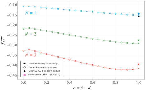
Figure 1: Free-energy density of the critical $\mathrm{O}(N)$ models for $N=1,2,3$ in $3\leq d\leq 4$ (i.e., $0\leq\varepsilon\leq 1$).

The method can be tested in $4d$ free scalar theory, $2d$ Ising model and in the large $N$ limit of the $\mathrm{O}(N)$ model, where numerical estimations can be compared with analytical results SM . In the following we apply it in the strongly-coupled regimes of the critical $\mathrm{O}(N)$ models for $N=1,2,3$. These correspond to the critical Ising model ($N=1$), the XY model ($N=2$), and the Heisenberg model ($N=3$), which are relevant for understanding ferromagnetism and other physical phenomena Berezinsky (1971); Kosterlitz and Thouless (1973); McBryan and Spencer (1977); Bitko et al. (1996). Our key results are: the free-energy density in $3\leq d\leq 4$ (Fig. 1), the two-point function of the lightest scalar in the critical $3d$ Ising model (Fig. 2), and the one-point functions of several operators in the critical $\mathrm{O}(1)$, $\mathrm{O}(2)$ and $\mathrm{O}(3)$ models (Figs. 3, 4). In the case of the $3d$ Ising model, our results can be compared with previous numerical estimates Iliesiu et al. (2019) and Monte Carlo simulations Vasilyev et al. (2009); Krech and Landau (1996); Krech (1997), confirming the validity of our method . The predictions for $N=2,3$ are new and could, in principle, be tested through further Monte Carlo simulations or experiments Lopes Cardozo et al. (2014).

Thermal bootstrap -

The starting point of our analysis is the KMS condition. For the two-point function of identical scalar operators $g(\tau)=\langle\phi(\tau)\phi(0)\rangle_{\beta}$, where the spatial distance between the two operators is set to zero, the KMS condition results into a tower of constraints that take the form

$$0=\frac{\partial^{m}}{\partial\tau^{m}}\left[g\left(\frac{\beta}{2}+\tau\right)-g\left(\frac{\beta}{2}-\tau\right)\right]_{\tau=0}\,,$$ (1)

where $m\in 2\mathbb{N}+1$. These constraints can be expressed as a set of sum rules Marchetto et al. (2024)

$$\sum_{\Delta}a_{\Delta}\ \mathtt{F}(\Delta,\Delta_{\phi},m)=0\,,$$ (2)

where the sum is performed over all the operators in the OPE between the two operators $\phi$. The kernel $\mathtt{F}$, defined in Eq. (9) in Marchetto et al. (2024), depends solely on zero-temperature CFT data, which we treat as input. Meanwhile, the coefficients $a_{\Delta}$ encode the thermal dynamical information

$$a_{\Delta}=\sum_{\mathcal{O}_{\Delta}}\frac{b_{\mathcal{O}}f_{\phi\phi\mathcal{O}}}{c_{\mathcal{O}}}\frac{J!}{2^{J}(\nu)_{J}}C_{J}^{\nu}(1)\,,$$ (3)

where the sum is performed over operators sharing the same scaling dimension, but with different spins. Here, the coefficients $f_{\phi\phi\mathcal{O}}$ and $c_{\mathcal{O}}$ correspond, respectively, to the structure constants and to the two-point function normalization of the operator $\mathcal{O}$ at zero temperature. $b_{\mathcal{O}}$ is the thermal one-point function coefficient defined via Iliesiu et al. (2018); Marchetto et al. (2023)

$$\langle\mathcal{O}_{\Delta}^{\mu_{1}\ldots\mu_{J}}\rangle_{\beta}=\frac{b_{\mathcal{O}}}{\beta^{\Delta}}(e^{\mu_{1}}\ldots e^{\mu_{J}}-\text{traces})\,.$$ (4)

The ultimate goal of the thermal bootstrap program is to compute these observables completing the set of thermal CFT data.

In order to solve the constraints (2), a naive approach consists in truncating the sum at a cut-off dimension $\Delta_{\text{max}}$. However this approach fails, as the contribution of the heavy operators cannot be discarded . This issue can be circumvented by approximating the tail of heavy operators using the asymptotic behavior of the coefficients $a_{\Delta}$ Marchetto et al. (2024)

$$a_{\Delta}^{\text{heavy}}=\frac{\Delta^{2\Delta_{\phi}-1}}{\Gamma(2\Delta_{\phi}+1)}\delta\Delta\left(1+\frac{c_{1}}{\Delta}+\ldots\right)\,.$$ (5)

Here, $\delta\Delta$ represents the gap between the scaling dimension $\Delta$ and the scaling dimension of the operator below it in the OPE spectrum. The coefficient $c_{1}$ is theory-dependent and corresponds to the first correction to the leading behavior. Let us comment that, in order to derive (5), it is necessary to add an analyticity assumption on $a_{\Delta}$, since the Tauberian theorem fixes only the leading term Marchetto et al. (2024). Moreover, note that the power of $\Delta$ in the first correction is universal, but this is not expected for higher corrections, where the power of $\Delta$ is theory-dependent. The constraints of Eq. (2) can be split into two terms:

$$\mathtt{f}(m)=\sum_{\Delta\leq\Delta_{\text{max}}}a_{\Delta}\mathtt{F}(\Delta,\Delta_{\phi},m)+\sum_{\Delta>\Delta_{\text{max}}}a_{\Delta}^{\text{heavy}}\mathtt{F}(\Delta,\Delta_{\phi},m)\,.$$ (6)

In this approximation, only a finite number of unknown coefficients are left: the coefficients $a_{\Delta}$ associated with the light operators $\Delta\leq\Delta_{\text{max}}$, and the corrections to the leading behavior (5), namely $c_{1}$, $\ldots$ . The constraints (2) can be formulated as the minimization of the cost function

$$\eta(\{\mathtt{\omega}_{i}\})=\sum_{m\leq m_{\text{max}}}\mathtt{\omega}_{m}\mathtt{f}(m)^{2}\,,$$ (7)

where $m_{\mathrm{max}}$ determines the maximum number of derivatives considered and $\omega_{i}\in(0,1)$ is a set of random number weights, which allows us to test the numerical stability of the algorithm as previously done, e.g., in Poland et al. (2024). The minimization process results in estimations for the unknown parameters, which are affected by numerical errors stemming from two contributions:

• A statistical error, estimated by the square root of the variance over multiple runs of the minimization of (7);

• A systematic error, due to the approximation of the contribution of the heavy operators using (5), estimated in SM .

Figure 2: The thermal two-point function $g(\tau)$ is shown alongside its KMS equivalent $g(\beta-\tau)$. The second plot shows the difference between the two curves in the main plot. We observe an excellent agreement in the region around the KMS fixed point ($\tau/\beta=1/2$).

The errors given in this letter should be understood as estimations and do not correspond to rigorous errors.

The free-energy density of the system is determined by the one-point function coefficient of the stress-energy tensor through $f=b_{T}/d$, with $d$ the number of spacetime dimensions Iliesiu et al. (2018). The structure constant $f_{\phi\phi T}$, appearing in (3), is fixed by the Ward identity and therefore

$$f=-a_{d}\frac{\Gamma\left(d/2\right)}{2\pi^{d/2}(d-1)\Delta_{\phi}}\frac{c_{T}}{c_{T,\,\text{free}}}\,,$$ (8)

where $c_{T,\,\text{free}}=d/(d-1)$. The method presented here can be tested on simple examples, and is found to produce accurate results for the free scalar field in $4d$, the $2d$ Ising model, and the $\mathrm{O}(N)$ model at large $N$ SM .

Ising, XY and Heisenberg models -

The method presented above can be used to study the $\mathrm{O}(N)$ model in $3\leq d\leq 4$. We consider in (2) the lightest scalar $\phi_{i}$ ($i=1,\ldots,N$) as external operator. We use two distinct sets of zero-temperature input: the results obtained from the $\varepsilon$-expansion and gathered in Henriksson (2023), and the results from the (zero-temperature) $3d$ bootstrap, given in El-Showk et al. (2012); Kos et al. (2016); Reehorst (2022); Chester et al. (2020); Liu et al. (2020); Chester et al. (2021) for $N=1,2,3$. To approximate the tail of heavy operators, we consider only the double-twist operators $[\phi\phi]_{n,\ell}$ in the second term of Eq. (6), corresponding to the identity by channel duality. The conformal dimensions of the double-twist operators can then be approximated by the mean-field theory results $\Delta_{n,\ell}=2\Delta_{\phi}+2n+\ell$. We consider the contribution of the identity operator and of the three lightest operators in the spectrum, and one correction to the Tauberian approximation SM . This results in four unknowns: the three non-trivial one-point functions and the correction to the Tauberian approximation $c_{1}$. All our calculations are performed by setting $m_{\text{max}}=7$ in (7), which corresponds to having four constraints of the type (2). Increasing $m_{\text{max}}$ would result in an increased error from the Tauberian approximation, which would in turn require the inclusion of additional corrections in (5).

Table 1: OPE coefficients $a_{\Delta}$ of light operators in the $3d$ Ising model, compared to Monte Carlo results (MC) and previous results (PR). The value for the Tauberian correction is $c_{1}\sim-0.065$, for which the error is negligible.

$\mathcal{O}$	$\Delta_{\mathcal{O}}$ Kos et al. (2016); Reehorst (2022)	This work	MC Vasilyev et al. (2009); Krech and Landau (1996); Krech (1997)	PR Iliesiu et al. (2019)
$\epsilon$	1.412625(10)	0.752(4)	0.711(3)	0.672(74)
$T_{\mu\nu}$	3	1.973(10)	2.092(13)	1.96(2)
$\epsilon^{\prime}$	3.82951(61)	0.1925(10)	0.17(2)	0.17(2)

We gather our results for the $3d$ Ising model ($N=1$) in Table 1 and compare them to the Monte-Carlo values and the previous results, which relied on a different thermal bootstrap approach. As already observed in Iliesiu et al. (2018), the value of the stress-energy tensor contribution is close to the large $N$ approximation, where $b_{T}\sim-0.459N$ and $a_{T}\sim 1.923$. The results obtained with the $\varepsilon$-expansion and the $3d$ conformal bootstrap as an input are shown in Fig. 1 for the free energy density. Notice that the error estimated on the coefficient $a_{d}$ propagates non-trivially on the free energy; in particular it is multiplied by $N$. We also estimated the thermal two-point function $g(\tau)$ by inputting the numerical results in the OPE: Fig. 2 shows a comparison between the two KMS-dual channels. The results for the OPE coefficients are presented in Fig. 3.

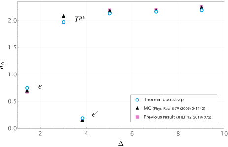
Figure 3: OPE coefficients for the lightest operators of the critical $3d$ Ising model.

Also for the XY model ($N=2$) many zero-temperature results have been obtained through the $\varepsilon$-expansion and the conformal bootstrap. We find the following predictions for the OPE coefficients in $3d$:

$$a_{\phi^{2}_{S}} =0.730(3) ( \Delta_{\phi^{2}_{S}}=1.51136(22))\,,$$ (9)

$$a_{T} =1.901(10) ( \Delta_{T}=3)\,,$$ (10)

$$a_{\phi^{4}_{S}} =0.2042(10) ( \Delta_{\phi^{4}_{S}}=3.794(8))\,.$$ (11)

The value for the Tauberian correction is $c_{1}\sim-0.0539$, for which the error is negligible. The free-energy density can be calculated using Eq. (8), and the results are shown in Fig. 1.

We performed the same calculations for the Heisenberg model ($N=3$), using the input from the $\varepsilon$-expansion and the conformal bootstrap. We obtain the following results for the OPE coefficients in $3d$:

$$a_{\phi^{2}_{S}} =0.763(4) ( \Delta_{\phi^{2}_{S}}=1.59489(59))\,,$$ (12)

$$a_{T} =1.815(9) ( \Delta_{T}=3)\,,$$ (13)

$$a_{\phi^{4}_{S}} =0.2069(10) ( \Delta_{\phi^{4}_{S}}=3.7668(100))\,.$$ (14)

The value for the Tauberian correction is $c_{1}\sim-0.0471$, for which the error is negligible. As for the other cases, we show the free-energy density in Fig. 1. The results for the OPE coefficients of the XY and the Heisenberg models are presented in Fig. 4. Note again that the results for $a_{T}$ for those models are very close to the large $N$ prediction.

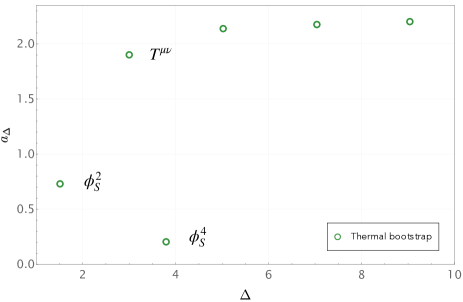
(a)

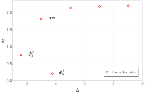
(b)

Figure 4: The two plots present the results for the OPE coefficients associated to the lightest operators of the OPE spectrum for the $\mathrm{O}(2)$ (left) and $\mathrm{O}(3)$ (right) models.

Discussion -

In this letter, we propose a numerical method for computing thermal OPE coefficients, which we apply to the critical $\mathrm{O}(N)$ models for $N=1,2,3$. In particular, we extract the free-energy density of the system in $3\leq d\leq 4$ as well as the OPE coefficients of the lightest operators. In the case of the $3d$ Ising model ($N=1$), our results can be compared with previous studies, while for $N=2,3$ we produce new predictions.

There are several directions to explore following this work. The methods presented here can be applied to different models. Motivated by recent progress in the context of holographic black holes Esper et al. (2023); Dodelson et al. (2024a); Bobev et al. (2023a); Dodelson et al. (2024b); Čeplak et al. (2024), it would be interesting to study the thermal $\mathcal{N}=4$ super Yang-Mills and ABJM theories, for which a plethora of zero-temperature CFT data is available in the literature Gromov et al. (2016, 2024); Chester et al. (2024); Aharony et al. (2008); Bobev et al. (2023b). Moreover, it was shown in Barrat et al. (2024) that the bootstrap problem in the presence of a temporal line defect is very similar to the one discussed in this letter. The exploration of this direction is crucial because of low-energy applications Affleck (1995); Sachdev (2010, 2024) and holographic interpretations Witten (1998). In the case of the Maldacena–Wilson line Maldacena (1998), a great amount of CFT data has been extracted recently Cavaglià et al. (2022a, b). The strategy of this letter could be adapted to all these configurations, which also provide a good stage for improving the precision on the numerical results Barrat et al. .

Finally, recently many different directions to study finite temperature effects in CFTs were proposed Petkou and Stergiou (2018); Petkou (2021); Benjamin et al. (2024a); Karydas et al. (2024); David and Kumar (2023, 2024); Benjamin et al. (2024b); Buric et al. (2024); Alkalaev and Mandrygin (2024). It would be interesting to compare and possibly incorporate these techniques with the method proposed in this paper.

References

- Sachdev (2011) S. Sachdev, Quantum Phase Transitions (Cambridge University Press, 2011).
- Vojta (2003) M. Vojta, Rept. Prog. Phys. 66, 2069 (2003).
- Witten (1998) E. Witten, Adv. Theor. Math. Phys. 2, 505 (1998), arXiv:hep-th/9803131 .
- Simmons-Duffin (2017) D. Simmons-Duffin, in Theoretical Advanced Study Institute in Elementary Particle Physics: New Frontiers in Fields and Strings (2017) pp. 1–74, arXiv:1602.07982 [hep-th] .
- Poland et al. (2019) D. Poland, S. Rychkov, and A. Vichi, Rev. Mod. Phys. 91, 015002 (2019), arXiv:1805.04405 [hep-th] .
- Rychkov and Su (2023) S. Rychkov and N. Su, (2023), arXiv:2311.15844 [hep-th] .
- El-Showk and Papadodimas (2012) S. El-Showk and K. Papadodimas, JHEP 10, 106 (2012), arXiv:1101.4163 [hep-th] .
- Iliesiu et al. (2018) L. Iliesiu, M. Koloğlu, R. Mahajan, E. Perlmutter, and D. Simmons-Duffin, JHEP 10, 070 (2018), arXiv:1802.10266 [hep-th] .
- Note (1) The OPE holds operatorially, though its radius of convergence is finite (and equal to ) at finite temperature.
- Kubo (1957) R. Kubo, J. Phys. Soc. Jap. 12, 570 (1957).
- Martin and Schwinger (1959) P. C. Martin and J. S. Schwinger, Phys. Rev. 115, 1342 (1959).
- Barrat et al. (2024) J. Barrat, B. Fiol, E. Marchetto, A. Miscioscia, and E. Pomoni, (2024), arXiv:2407.14600 [hep-th] .
- Note (2) The KMS fixed point is achieved when the two operators are placed at an imaginary time separation of .
- Marchetto et al. (2024) E. Marchetto, A. Miscioscia, and E. Pomoni, JHEP 09, 044 (2024), arXiv:2312.13030 [hep-th] .
- (15) See Supplemental Material.
- Berezinsky (1971) V. L. Berezinsky, Sov. Phys. JETP 32, 493 (1971).
- Kosterlitz and Thouless (1973) J. M. Kosterlitz and D. J. Thouless, J. Phys. C 6, 1181 (1973).
- McBryan and Spencer (1977) O. A. McBryan and T. Spencer, Commun. Math. Phys. 53, 299 (1977).
- Bitko et al. (1996) D. Bitko, T. F. Rosenbaum, and G. Aeppli, Phys. Rev. Lett. 77, 940 (1996).
- Iliesiu et al. (2019) L. Iliesiu, M. Koloğlu, and D. Simmons-Duffin, JHEP 12, 072 (2019), arXiv:1811.05451 [hep-th] .
- Vasilyev et al. (2009) O. Vasilyev, A. Gambassi, A. Maciołek, and S. Dietrich, Phys. Rev. E 79, 041142 (2009).
- Krech and Landau (1996) M. Krech and D. P. Landau, Phys. Rev. E 53, 4414 (1996).
- Krech (1997) M. Krech, Phys. Rev. E 56, 1642 (1997).
- Note (3) Thermal OPE coefficients from Monte Carlo simulations require combining simulation results with the inversion formula, as done for the Ising model in Iliesiu et al. (2019).
- Lopes Cardozo et al. (2014) D. Lopes Cardozo, H. Jacquin, and P. C. W. Holdsworth, Phys. Rev. B 90, 184413 (2014).
- Marchetto et al. (2023) E. Marchetto, A. Miscioscia, and E. Pomoni, JHEP 12, 186 (2023), arXiv:2306.12417 [hep-th] .
- Note (4) The error introduced by neglecting the tail of heavy operators is shown in Marchetto et al. (2024). This is very different from the zero-temperature scenario, since in such case the naive truncation of the crossing equations can still lead to reasonably good approximations Gliozzi (2013); Gliozzi and Rago (2014); Gliozzi (2016). Nevertheless, the tail of heavy operators is still important to achieve a higher precision, as shown by Su (2022); Li (2024); Poland et al. (2024). In particular, in Li (2024); Poland et al. (2024) the authors employ a procedure similar to ours for the estimation of the error.
- Poland et al. (2024) D. Poland, V. Prilepina, and P. Tadić, JHEP 05, 299 (2024), arXiv:2312.13344 [hep-th] .
- Note (5) We exclude the case in which there are more operators of dimension . This is the case for the model that we are studying in this letter.
- Note (6) We use conformal dimensions up to order and the CFT data needed to convert the stress-energy tensor coefficient to free energy up to order .
- Henriksson (2023) J. Henriksson, Phys. Rept. 1002, 1 (2023), arXiv:2201.09520 [hep-th] .
- El-Showk et al. (2012) S. El-Showk, M. F. Paulos, D. Poland, S. Rychkov, D. Simmons-Duffin, and A. Vichi, Phys. Rev. D 86, 025022 (2012), arXiv:1203.6064 [hep-th] .
- Kos et al. (2016) F. Kos, D. Poland, D. Simmons-Duffin, and A. Vichi, JHEP 08, 036 (2016), arXiv:1603.04436 [hep-th] .
- Reehorst (2022) M. Reehorst, JHEP 09, 177 (2022), arXiv:2111.12093 [hep-th] .
- Chester et al. (2020) S. M. Chester, W. Landry, J. Liu, D. Poland, D. Simmons-Duffin, N. Su, and A. Vichi, JHEP 06, 142 (2020), arXiv:1912.03324 [hep-th] .
- Liu et al. (2020) J. Liu, D. Meltzer, D. Poland, and D. Simmons-Duffin, JHEP 09, 115 (2020), [Erratum: JHEP 01, 206 (2021)], arXiv:2007.07914 [hep-th] .
- Chester et al. (2021) S. M. Chester, W. Landry, J. Liu, D. Poland, D. Simmons-Duffin, N. Su, and A. Vichi, Phys. Rev. D 104, 105013 (2021), arXiv:2011.14647 [hep-th] .
- Esper et al. (2023) C. Esper, K.-W. Huang, R. Karlsson, A. Parnachev, and S. Valach, JHEP 11, 107 (2023), arXiv:2306.00787 [hep-th] .
- Dodelson et al. (2024a) M. Dodelson, C. Iossa, R. Karlsson, and A. Zhiboedov, JHEP 01, 036 (2024a), arXiv:2304.12339 [hep-th] .
- Bobev et al. (2023a) N. Bobev, J. Hong, and V. Reys, JHEP 12, 054 (2023a), arXiv:2309.06469 [hep-th] .
- Dodelson et al. (2024b) M. Dodelson, C. Iossa, R. Karlsson, A. Lupsasca, and A. Zhiboedov, JHEP 07, 046 (2024b), arXiv:2310.15236 [hep-th] .
- Čeplak et al. (2024) N. Čeplak, H. Liu, A. Parnachev, and S. Valach, JHEP 10, 105 (2024), arXiv:2404.17286 [hep-th] .
- Gromov et al. (2016) N. Gromov, F. Levkovich-Maslyuk, and G. Sizov, JHEP 06, 036 (2016), arXiv:1504.06640 [hep-th] .
- Gromov et al. (2024) N. Gromov, A. Hegedus, J. Julius, and N. Sokolova, JHEP 05, 185 (2024), arXiv:2306.12379 [hep-th] .
- Chester et al. (2024) S. M. Chester, R. Dempsey, and S. S. Pufu, JHEP 07, 059 (2024), arXiv:2312.12576 [hep-th] .
- Aharony et al. (2008) O. Aharony, O. Bergman, D. L. Jafferis, and J. Maldacena, JHEP 10, 091 (2008), arXiv:0806.1218 [hep-th] .
- Bobev et al. (2023b) N. Bobev, J. Hong, and V. Reys, JHEP 02, 020 (2023b), arXiv:2210.09318 [hep-th] .
- Affleck (1995) I. Affleck, Acta Phys. Polon. B 26, 1869 (1995), arXiv:cond-mat/9512099 .
- Sachdev (2010) S. Sachdev, J. Stat. Mech. 1011, P11022 (2010), arXiv:1010.0682 [cond-mat.str-el] .
- Sachdev (2024) S. Sachdev (2024) arXiv:2407.15919 [cond-mat.str-el] .
- Maldacena (1998) J. M. Maldacena, Phys. Rev. Lett. 80, 4859 (1998), arXiv:hep-th/9803002 .
- Cavaglià et al. (2022a) A. Cavaglià, N. Gromov, J. Julius, and M. Preti, Phys. Rev. D 105, L021902 (2022a), arXiv:2107.08510 [hep-th] .
- Cavaglià et al. (2022b) A. Cavaglià, N. Gromov, J. Julius, and M. Preti, JHEP 05, 164 (2022b), arXiv:2203.09556 [hep-th] .
- (54) J. Barrat, E. Marchetto, A. Miscioscia, and E. Pomoni, work in progress.
- Petkou and Stergiou (2018) A. C. Petkou and A. Stergiou, Phys. Rev. Lett. 121, 071602 (2018), arXiv:1806.02340 [hep-th] .
- Petkou (2021) A. C. Petkou, Phys. Lett. B 820, 136467 (2021), arXiv:2105.03530 [hep-th] .
- Benjamin et al. (2024a) N. Benjamin, J. Lee, H. Ooguri, and D. Simmons-Duffin, JHEP 03, 115 (2024a), arXiv:2306.08031 [hep-th] .
- Karydas et al. (2024) M. Karydas, S. Li, A. C. Petkou, and M. Vilatte, Phys. Rev. Lett. 132, 231601 (2024), arXiv:2312.00135 [hep-th] .
- David and Kumar (2023) J. R. David and S. Kumar, JHEP 10, 143 (2023), arXiv:2307.14847 [hep-th] .
- David and Kumar (2024) J. R. David and S. Kumar, (2024), arXiv:2406.14490 [hep-th] .
- Benjamin et al. (2024b) N. Benjamin, J. Lee, S. Pal, D. Simmons-Duffin, and Y. Xu, (2024b), arXiv:2405.17562 [hep-th] .
- Buric et al. (2024) I. Buric, F. Russo, V. Schomerus, and A. Vichi, (2024), arXiv:2408.02747 [hep-th] .
- Alkalaev and Mandrygin (2024) K. B. Alkalaev and S. Mandrygin, (2024), arXiv:2407.01741 [hep-th] .
- (64) H. Helton, MSc Thesis, Princeton University .
- Gliozzi (2013) F. Gliozzi, Phys. Rev. Lett. 111, 161602 (2013), arXiv:1307.3111 [hep-th] .
- Gliozzi and Rago (2014) F. Gliozzi and A. Rago, JHEP 10, 042 (2014), arXiv:1403.6003 [hep-th] .
- Gliozzi (2016) F. Gliozzi, JHEP 10, 037 (2016), arXiv:1605.04175 [hep-th] .
- Su (2022) N. Su, (2022), arXiv:2202.07607 [hep-th] .
- Li (2024) W. Li, JHEP 07, 047 (2024), arXiv:2312.07866 [hep-th] .