Can dark energy explain a high growth index?

Abstract

A promising way to test the physics of the accelerated expansion of the Universe is by studying the growth rate of matter fluctuations, which can be parameterized by the matter energy density parameter to the power $\gamma$, the so-called growth index. It is well-known that the $\Lambda$CDM cosmology predicts $\gamma=0.55$. However, using observational data, Ref. [1] measured a much higher $\gamma=0.633^{+0.025}_{-0.024}$, excluding the $\Lambda$CDM value within $3.7\sigma$. In this work, we analyze whether Dark Energy (DE) with the Equation of State (EoS) parameter described by the CPL parametrization can significantly modify $\gamma$ with respect to the $\Lambda$CDM one. Besides the usual Smooth DE (SDE) scenario, where DE perturbations are neglected on small scales, we also consider the case of Clustering Dark Energy (CDE), which has more potential to impact the growth of matter perturbations. In order to minimally constrain the background evolution and assess the largest meaningful $\gamma$ distribution, we use data from $32$ Cosmic Chronometers, $H(z$), data points. In this context, we found that both SDE and CDE models described by the CPL parametrization can not provide a significant number of $\gamma$ samples compatible with the value determined in Ref. [1]. Therefore, explaining the measured value of $\gamma$ is a challenge for DE models. Moreover, we present new fitting functions for $\gamma$, which are more accurate and general than the one proposed in Ref. [2] for SDE, and, for the first time, fitting functions for CDE models.

I Introduction

The accelerated expansion of the universe is still a big question in Cosmology. It can be explained either by a modified theory of gravity, or a unknown component of the universe, labeled as Dark Energy (DE) [3]. In the pursue of more accurate data to answer this question, some tensions arose. The most significant one is known as the Hubble tension, which reflects the difference between measurements of the present expansion rate, $H_{0}$, obtained locally by using the distance ladder methods [4] and globally, assuming the $\Lambda$CDM model, from Cosmic Microwave Background (CMB) data [5]. There is also the $S_{8}$ tension (where $S_{8}\equiv\sigma_{8}\sqrt{\Omega_{m0}/0.3}$, $\sigma_{8}$ is the amplitude of matter fluctuations at $8h^{-1}\text{Mpc}$ and $\Omega_{m0}$ is the matter density parameter now), which is related to the difference between the values of these parameters inferred from CMB [5] and measurements of galaxy clustering and weak gravitational lensing, as discussed in [6].

The $S_{8}$ tension is directly related to the growth of cosmic perturbations. A particular simple and promising way to test how the physics of the accelerated expansion impacts the evolution of matter perturbations is by analyzing the growth rate of matter perturbations [7]

$$f=\frac{d\ln\delta_{m}}{d\ln a}\,,$$ (1)

which can be parametrized as [2]

$$f\simeq\Omega_{m}^{\gamma}\,,$$ (2)

where $\gamma$ is a constant that depends weakly on the Equation of State (EoS) parameter of Smooth DE (SDE) models, $w\left(t\right)=p_{de}\left(t\right)/\rho_{de}\left(t\right)$, and $\Omega_{m}=\Omega_{m}\left(a\right)$ is the matter energy density parameter. For the $\Lambda$CDM cosmology, Refs. [8, 2] found $\gamma=0.55$. However, using observational data, Ref. [1] found a much higher $\gamma=0.633$ (implying a suppression of growth), excluding the $\Lambda$CDM value by $3.7\sigma$. In the same work, it was also shown that a higher $\gamma$ values reduces the $S_{8}$ tension from $3.2\sigma$ to $0.9\sigma$.

This high value of $\gamma$ naturally raises the question of what theoretical mechanisms are capable of producing it. In the case of SDE, it was shown that $\gamma$ can be accurately described by the fitting function [2],

$$\gamma(w_{1})=\begin{cases}0.55+0.02(1+w_{1}),&w_{1}\leq-1\\ 0.55+0.05(1+w_{1}),&w_{1}>-1\end{cases},$$ (3)

where $w_{1}=w\left(z=1\right)$. This indicates that, for $w_{1}\leq-1$, we would need $w_{1}=3.15$ to get $\gamma=0.633$, in contradiction with the parametrization condition. For $w_{1}>-1$, we would need $w_{1}=0.66$, which would generate a large DE density around $z=1$. This simple extrapolation exercise indicates that it should be very difficult for SDE models to produce a high growth index. As we will show, with very loose constraints on the background evolution based on Cosmic Chronometers (CC) data, SDE with CPL parametrization has an almost negligible probability of producing $\gamma>0.6$.

The usual assumption of SDE, in which one usually neglects DE perturbations on small scales, is based on Quintessence models [9, 10, 11]. In this case, DE is described by a minimally coupled canonical scalar field. The linear perturbations of this field propagate with sound speed $c_{s}=1$, not allowing its perturbations to grow significantly on small scales. This approximation is well justified even in the nonlinear regime [12]. The simplest generalization of this scenario can be done by describing DE as a non-canonical minimally coupled scalar field, called k-essence [13, 14]. In this case, $c_{s}$ can be chosen and DE pertubations can grow at small scales, see [15] for a more detailed discussion. In this work, we will consider the limiting case of $c_{s}\rightarrow 0$, in which DE pertubations have the maximal potential to grow and impact the evolution of matter perturbations. We refer to this scenario as Clustering DE (CDE), which growth index has already been studied in [16, 17, 18, 19].

In this paper, we explore how SDE and CDE can change the growth index. We confirm the expectation based on the fitting formula (3) that SDE model can not provide $\gamma\simeq 0.633$. We also find that CDE models can not raise the values of $\gamma$ significantly, therefore concluding that DE models are quite challenged by observed value of $\gamma$.

As we will show, for the case of CDE, this result has a simple explanation. When $w\left(t\right)>-1$, DE perturbations are have the tendency of being correlated with matter perturbations ($\delta_{de}\propto\delta_{m}$) and anti-correlated for $w\left(t\right)<-1$ ($\delta_{de}\propto-\delta_{m}$). In other to raise $\gamma$, DE perturbations must be anti-correlated with $\delta_{m}$, causing a decrease in the gravitational potential and consequently slowing down the growth rate (higher $\gamma$). However, in the case $w\left(t\right)<-1$, the DE energy density decreases rapidly at high-$z$, thus the overall impact is very limited. On the other hand, the case $w\left(t\right)>-1$ can easily enhance the matter growth, thus providing a significantly lower $\gamma$ values, as already shown in [16].

Based on the samples of $\gamma$ that we have computed, we where able to construct a new parametrization $\gamma=$$\gamma\left(w_{1}\right)$, which is more accurate than (3) and valid for larger parameter space. Moreover, for the first time, we present a $\gamma$ parametrization for the case of CDE.

The plan of this paper is as follows. In Sect. II, we define the background cosmology, the data, the parameters priors and statistics used to constrain the background evolution. In Sect. III, we present the equations for the evolution of matter and DE pertubations. The results of the sampling, analysis and suitable fittings are shown in Sect. IV and the conclusions are organized in Sect. V.

II Background cosmology

In this work, we assume General Relativity and a flat universe described Friedmann-Lemaître-Robertson-Walker metric, in which the line element is represented by

$$ds^{2}=-c^{2}dt^{2}+a(t)^{2}\left[dr^{2}+r{}^{2}d\Omega^{2}\right],$$ (4)

where $a(t)$ is the scale factor. As so, the square of the Hubble function can be written as

$$H^{2}=\left(\frac{\dot{a}}{a}\right)^{2}=H_{0}^{2}\left(\Omega_{m0}a^{-3}+\Omega_{de}\left(a\right)\right)\,,$$ (5)

where $\Omega_{m0}$ is the matter (dark matter plus baryons) density parameter now and $\Omega_{de}\left(a\right)$ is the DE energy parameter, which depends on the EoS assumed.

We consider that DE EoS is given by Chevallier-Polarski-Linder (CPL) [20, 21] parametrization:

$$w(a)=w_{0}+w_{a}(1-a).$$ (6)

Thus, the DE density parameter is given by

$$\Omega_{de}(a)=(1-\Omega_{m0})a^{-3(1+w_{0}+w_{a})}\exp\left(-3w_{a}(1-a)\right).$$ (7)

Besides the general case of free $w_{0}$ and $w_{a}$, we will also analyze the $\Lambda$ limit ($w_{0}=-1$ and $w_{a}=0$) and constant EoS case (free $w\equiv w_{0}$ and $w_{a}=0$). We refer to these models as CPL, $\Lambda$CDM and $w$CDM, respectively. In the general case, we have four free parameters: $h=H_{0}/\left(100\text{km s}^{-1}\text{Mpc}^{-1}\right)$, $\Omega_{m0}$, $w_{0}$ and $w_{a}$. Next, we discuss how to minimally constrain these parameters using $H\left(z\right)$ data.

Cosmic Chronometers Data

In order to minimally constraint the background evolution and the model parameters, we make use 32 of the most recent CC data available, compiled by [22]. We use the Python library Emcee [23] as a Monte Carlo Markov Chain (MCMC) sampler and Python library GetDist [24] to analyse and plot the posteriors distributions.

There is a well-know discussion about the systematic errors in CC data, [25, 26, 27]. In these works, systematics of 15 of the 32 data points have been analyzed. Here, we split the data set in two groups (with and without systematics), and $\chi^{2}$ given by

$$\chi^{2}=\chi_{{\rm nosys}}^{2}+\chi_{{\rm sys}}^{2}\,,$$ (8)

where $\chi_{{\rm nosys}}^{2}$ is associated with the 17 data-points without systematics, provided by [28, 29, 30, 31, 32, 33], which reads

$$\chi_{{\rm nosys}}^{2}=\sum_{i}\left(\frac{\Delta H_{i}}{\sigma_{i}}\right)^{2}\,,$$ (9)

where $\Delta H_{i}=H_{\text{model}}\left(z_{i}\right)-H_{{\rm\text{data}}}\left(z_{i}\right)$ and $\sigma_{i}$ is the corresponding uncertainty of data points. The other part of the $\chi^{2}$ associated with data points with systematics is given by

$$\chi_{{\rm sys}}^{2}=\Delta\vec{H}^{T}\boldsymbol{Cov}^{-1}\Delta\vec{H}\,,$$ (10)

where $\Delta\vec{H}$ is a vector with $\Delta H_{i}$ components associated the 15 data points provided by Refs. [25, 26, 27], and $\boldsymbol{Cov}$ is the corresponding covariance matrix for BC3 model, available at https://gitlab.com/mmoresco/CCcovariance.

We sample the posterior distribution of the vector of parameters $\theta=\left(h,\Omega_{m0},w_{0},w_{a}\right)$, given by

$$\mathcal{L}\left(\theta|D\right)\propto P\left(\theta\right)L\left(D|\theta\right)\,,$$ (11)

where

$$L\left(D|\theta\right)\propto\exp\left(-\frac{\chi^{2}}{2}\right)$$ (12)

is the likelihood of the data $D$ given $\theta$ and $P\left(\theta\right)$ indicates the priors assumed for the parameters, listed in Tab. 1. We also implement an additional flat prior to exclude cosmologies in which $\Omega_{de}\left(z=1000\right)>0.01$, where $z=1/a-1$ is the redshift. This condition is similar to the assumption $w_{0}+w_{a}<-0.1$ described by [34]. Allowing for DE models with non-negligible energy density at high-$z$, besides being highly disfavored by data [35], invalidates the Einstein-de-Sitter initial conditions used to solve the evolution of matter and DE perturbations, which will be discussed in detail in the next section.

Table 1: Priors for all parameters.

Parameter	Prior
$h$	$\mathcal{U}[0.5,1]$
$\Omega_{m0}$	$\mathcal{U}[0.01,0.99]$
$w$	$\mathcal{U}[-3,-1/3]$
$w_{0}$	$\mathcal{U}[-3,1]$
$w_{a}$	$\mathcal{U}[-3,3]$

The results for $\Lambda$CDM, $w$CDM and CPL models are presented in figures 1, 2 and 3, respectively. Regarding the background parameters, we can see in Fig. 1 that CC data can constraint the two free parameters, $\Omega_{m0}$ and $h$, in the $\Lambda$CDM model. For $w$CDM this is not case, mainly because $w$ is being limited by the prior assumed, but note that the posterior also shows some preference for $w\simeq-1$. Fig. 3 also shows that CPL parameters, $w_{0}$ and $w_{a}$, can not be constrained by CC data. The posteriors of $w_{0}$ and $w_{a}$ are dominated by the flat priors shown in table 1 together with the condition $\Omega_{de}\left(z=1000\right)<0.01$. The mean values for the marginalized 1D distributions are given in Tab. 2. The number of samples in our chains is $N\sim 1000\tau$, where $\tau$ is the largest auto-correlation time of the parameters. This is well beyond the suggested $N>50\tau$ described in [23] as convergence criteria.

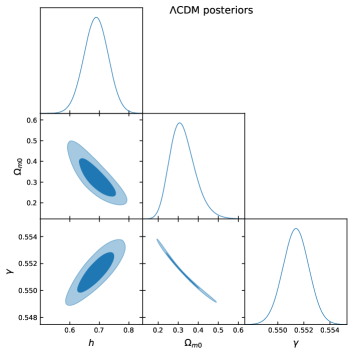
Figure 1: Marginalized posterior distributions for the $\Lambda$CDM model parameters.

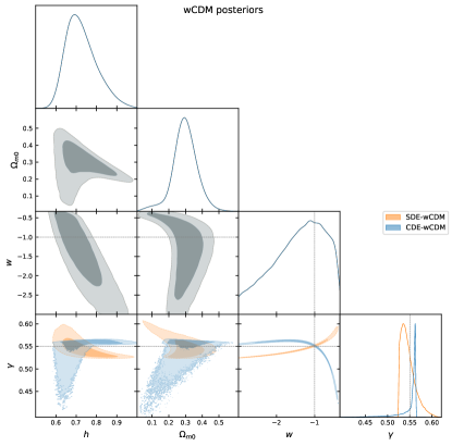
Figure 2: Marginalized posterior distributions for the $w$CDM models, with a shared background and distinct Smooth and Clustering Dark Energy growth index distributions. The dashed lines indicate the values of the $\Lambda$CDM parameters.

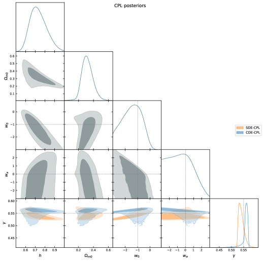
Figure 3: Marginalized posterior distributions for the CPL models, with a shared background and distinct Smooth and Clustering Dark Energy growth index distributions. The dashed lines indicate the values of the $\Lambda$CDM parameters.

We recall that the main purpose of this analysis is to provide a wide, but still meaningful, distribution of background parameters that can be used to compute the linear growth of matter perturbations and $\gamma$. As we will see, despite this large variation of the EoS parameters, $\gamma$ can be determined with much smaller variation. In the next section we describe the perturbative equations for SDE and CDE models.

III Growth of Cosmological Perturbations

In a universe with SDE, the linear evolution of the matter density contrast, $\delta_{m}\equiv\rho_{m}/\overline{\rho}_{m}-1$, is solely affected by the background expansion, as described by the equation

$$\delta_{m}^{\prime\prime}+\left(2-\frac{1+3w\left(a\right)\Omega_{de}\left(a\right)}{2}\right)\frac{\delta_{m}^{\prime}}{a}-\frac{3}{2}\frac{\Omega_{m}\left(a\right)}{a^{2}}\delta_{m}=0,$$ (13)

where the prime denotes a derivative with respect to the scale factor. Starting the integration at a high redshift, $z_{i}=1000$, initial values can be computed using the analytical solution for a matter-dominated Einstein-de-Sitter (EdS) universe $\delta_{mi}^{\prime}=\delta_{mi}/a_{i}$, where we assumed $\delta_{mi}>0$.

In the case of CDE, $\delta_{m}$ is also affected by DE perturbations, $\delta_{de}$, whose effect is maximized for DE models with negligible sound speed. In this work, we consider the extreme case $c_{s}=0$ based on the fluid description of DE and phenomenologically allowing for EoS which can be non-phantom ($w(t)>-1$), phantom ($w(t)<-1$) or transit between these regimes. In this context, matter and DE perturbations obey the following system of equations [15]:

$$\begin{cases}\delta_{m}^{\prime}+\frac{q}{a^{2}}&=0\,,\\ \delta_{de}^{\prime}-3\frac{w}{a}\delta_{de}+(1+w)\frac{q}{a^{2}}&=0\,,\\ q^{\prime}-\frac{1}{2}(1+3w\Omega_{de})\frac{q}{a}+\frac{3}{2}(\Omega_{m}\delta_{m}+\Omega_{de}\delta_{de})&=0\,,\end{cases}$$ (14)

where $q\equiv\theta/H$ and $\theta=\vec{\nabla}\cdot\vec{v}$ is the divergence of the peculiar velocity of the DE-matter fluid. Note that the equation for the peculiar velocity is the same for matter and CDE because we are considering $c_{s}=0$. To compute the initial conditions for DE perturbations, we use the solution valid for constant $w$ in matter-dominated era [36, 37, 38, 39]

$$\delta_{de}=\frac{1+w}{1-3w}\delta_{m}.$$ (15)

Although solution (15) only gives a general qualitative behavior at low-$z$ [39], it can help us to predict the influence of CDE on the growth of $\delta_{m}$. When $w\left(a\right)<-1$ we have the tendency $\delta_{de}\propto-\delta_{m}$, while for $w\left(a\right)>-1$ we have $\delta_{de}\propto\delta_{m}$. If the EoS is always phantom or non-phanton, these relations are always valid. In the case that the EoS transits between phantom and non-phanton or vice-versa, the actual relation between $\delta_{de}$ and $\delta_{m}$ might take some time to achieve the expected behavior. The general trend is clear: phantom EoS will induce negative $\delta_{de}$, lowering the clustering power encoded in the last term of Eq. (14), whereas non-phantom EoS enhances growth. Therefore, the desired higher values of $\gamma$ could be obtained in phantom CDE models.

We solve Eqs. (13) and (14), then determine the growth rate $f=d\ln\delta_{m}/d\ln a$ and fit a constant $\gamma$ assuming $f=\Omega_{m}^{\gamma}(a)$ for all the posterior distribution obtained and the measured value. In this process, it is important to ask whether the fitted values of $\gamma$ can accurately describe $f$. In the paper [2], where the fit (3) was introduced for the SDE model described by CPL parametrization, the accuracy of the fit was reported with respect to the growth variable $g\equiv\delta/a$. Accuracies better than $0.05\%$ for $\Lambda$CDM with $\Omega_{m0}\in[0.22,1]$ were reported, and $1\%$ when lowering the limit to $\Omega_{m0}=0.01$. For $w\neq-1$, the paper reported an accuracy within $0.4\%$ for $w=-0.5$ and for dynamical EoS $0.25\%$ when $w_{0}=-0.82$ and $w_{a}=0.58$. Here, we first will check how accurately a constant $\gamma$ can reproduce $f$. In the next section, we will propose and analyze a new fitting function for $\gamma$.

In this work, we report the distribution of percent residuals given by the Root Mean Square (RMS) of $1-\Omega_{m}^{\gamma_{{\rm nun}}}\left(z\right)/f_{{\rm nun}}\left(z\right)$, where $f_{{\rm nun}}$ is the numerical solution and $\gamma_{{\rm nun}}$ the corresponding fitted gamma value. We compute the RMS percent residuals along $10$ evenly spaced values of $0\leq z\leq 2$, and show its distribution in Fig. 4. As can be seen, a very small fraction of models have residuals greater than $0.5\%$. The worst case occurs for CDE-CPL, reaching up to $4\%$, but still for a small fraction of the realizations. In general, all models present a concentration of residuals close to $0.15\%$. We also have checked that the largest residuals are mainly associated with low $\Omega_{m0}$ values. This demonstrates that, considering the CPL EoS, the constant $\gamma$ parametrization for the growth rate is very reliable, even in the case of CDE. However, for more complex EoS parametrizations and for realizations including a non-negligible DE density at high-$z$, the constant $\gamma$ parametrization might not be adequate [16].

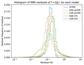
Figure 4: Histogram of RMS percent residuals for the constant growth index fit, with respect to the numerical solution of $f$ for each model, normalized by relative frequency.

IV Results for $\gamma$

The $\Lambda$CDM posteriors shown in Fig. 1 display a great determination of the growth index at $\gamma_{\Lambda}=0.5514\pm 0.0010$, agreeing with the previous results from Refs. [8, 2]. However, using data from Cosmological Microwave Background, galaxy surveys and Baryon Acoustic Oscillation data, Ref. [1] found a value of $\gamma_{m}=0.633_{-0.024}^{+0.025}$, excluding the $\Lambda$CDM value within $3.7\sigma$, also showing that this value effectively solves the $S_{8}$ tension. Assuming normally distributed probabilities for the measured value and the $\Lambda$CDM one, with mean and standard deviation given in Tab. 2, a simply quantification of the tension between these values is given by

$$\#\sigma=\frac{|\gamma_{m}-\gamma_{\Lambda}|}{\sqrt{\sigma_{m}^{2}+\sigma_{\Lambda}^{2}}}=3.26\,$$ (16)

where we used $\sigma_{m}=0.025$. If we assume the usual value $\gamma_{\Lambda}=0.55$ and neglect its uncertainty, we get $3.32\sigma$.

Now let us check whether more general SDE models and their CDE counterparts can explain the observed value. Although the analysis in Ref. [1] assumes the $\Lambda$CDM background to produce the $\gamma$ constraints, assessing the possible values of $\gamma$ in more general background and perturbative models will help us to identify scenarios in which $\gamma$ can be increased and how likely this can happen.

We first analyze the correlations between the $\gamma$ and the EoS parameters and how $\gamma$ changes with respect to the $\Lambda$CDM value. The clearest case is for $w$CDM model, Fig. 2, but the following analysis also holds for CPL model. For $w>-1$ (non-phantom EoS) we have lower $\Omega_{m}\left(z\right)$ in the past with respect to the $w=-1$ case. In the SDE scenario, this behavior causes a suppression of growth, giving a higher $\gamma$. In the case of CDE, this correlation is inverted because $w>-1$ induces positive $\delta_{de}$, which will act as an extra source of the gravitational potential, enhancing the growth and lowering $\gamma$. For $w<-1$ (phantom EoS) we have higher $\Omega_{m}\left(z\right)$ in the past with respect to $w=-1$. In SDE case, this induces a lower $\gamma$. Again, CDE inverts this correlation because now negative $\delta_{de}$ is induced, reducing the source of the gravitational potential, consequently increasing $\gamma$. These correlations also hold for CPL, but since many realizations shown in Fig. 3 include transitions from phantom to non-phantom EoS and vice-versa, they are not very clearly visualized. However, in terms of $w_{1}$, these correlations become more evident in Fig. 7. Therefore we can summarize impact of DE model in the $\gamma$ , with respect to the $\Lambda$CDM value, as follows:

• SDE, non-phantom EoS: $\gamma>0.55$

• SDE, phantom EoS: $\gamma<0.55$

• CDE, non-phantom EoS: $\gamma<0.55$

• CDE, phantom EoS: $\gamma>0.55$

It is also interesting to check the frequency of positive or negative occurrences of $\delta_{de}$ for the CDE scenario. In Fig. 5, we present the distribution of $\delta_{de}/\delta_{m}$ at $z=0$ and $z=0.5$. We can see a small preference for negative $\delta_{de}$, which is associated with the allowed values of the EoS parameters as follows. For non-phantom EoS, $\Omega_{de}\left(z\right)$ can be large at intermediate and high-$z$, a situation that is disfavored by data, e.g., [35]. In our analysis, this fact is mainly implemented with the prior $\Omega_{de}\left(z=1000\right)<0.01$. On the other hand, for phantom EoS, $\Omega_{de}\left(z\right)$ is very small at intermediate and high-$z$ and can still can induce an adequate accelerated expansion at low-$z$. Therefore, the allowed parameter space for the EoS parameters has a larger fraction of phantom realizations. As a consequence, given the correlations between $w$ and $\delta_{de}$ explained earlier, we see some preference for $\delta_{de}<0$.

Figure 5: Distribution of perturbation ratios for $w$CDM and CPL models at $z=0$ (left panel) and $z=0.5$ (right panel).

In Fig. 6 we show a direct comparison between the $\gamma$ distributions obtained. As can be seen, the SDE models are similar, regardless of the EoS parametrization. The same happens for the CDE models. Given the larger fraction of phantom realizations, SDE models have a slight preference for $\gamma<0.55$, whereas CDE prefers $\gamma>0.55$. The $\gamma$ distributions for non-$\Lambda$ models have greater variance and asymmetry. However, none of these models provide a significant fraction of realizations around $\gamma\simeq 0.633$.

Considering the $2\sigma$ lower limit of the measured value as $\gamma_{\rm min}=0.633-2\cdot 0.025=0.583$, only the SDE-$w$CDM model has values higher than this, what happens only above percentile 96 of its $\gamma$ distribution. If we cut this $\gamma$ distribution with $\Omega_{m0}>0.2$, $\gamma_{\rm min}$ occurs only above percentile 99. As can be seen in Fig. 6, all the other models have much smaller probabilities of producing $\gamma_{\rm min}$.

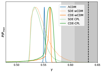
Figure 6: Distribution for $\gamma$ in different models. The vertical dashed line marks the measured value $\gamma=0.633$, the grey bands indicate its $1\sigma$ and $2\sigma$ intervals, assuming a normal distribution.

We could expect that phantom CDE models are able to produce high $\gamma$ values because, as explained earlier, the associated negative $\delta_{de}$ operates in this direction. However, given that the gravitational potential depends on $\Omega_{de}\delta_{de}$ and, in the phantom case, $\Omega_{de}$ is small at intermediate and high-$z$, the actual impact of these models on $\gamma$ is very limited. Consequently, although some preference for $\gamma>0.55$ can be seen in Fig. 6, the highest possible values virtually never reach $\gamma\gtrsim 0.58$.

Therefore, our main result is that both SDE and CDE models described by the CPL EoS parametrization have very small probabilities of providing a growth index compatible with close to $\gamma=0.633^{+0.025}_{-0.024}$, found in Ref. [1]. Bear in mind that in order to produce the $\gamma$ distributions we only used CC data, the priors in Tab. 1 and the condition $\Omega_{de}\left(z=1000\right)<0.01$. Therefore, adding more background data in the analysis can only constrain more the parameter space and consequently the $\gamma$ distribution.

The mean values for the marginalized 1D distributions are listed in Tab. 2. Note that, as the $\gamma$ distribution is heavy tailed for CDE models, and reported mean value can lie outside the $1\sigma$ interval. We verified that the best fit model parameters lie within $1\sigma$ of the 1D marginalized distributions.

Table 2: Marginalized 1D constraints and $68\%$ C.L. intervals for the parameters of each cosmology.

Parameter	$\Lambda$CDM	$w$CDM	CPL
$h$	$0.689\pm 0.041$	$0.727_{-0.092}^{+0.054}$	$0.733_{-0.10}^{+0.069}$
$\Omega_{m0}$	$0.324_{-0.072}^{+0.049}$	$0.296\pm 0.076$	$0.319_{-0.082}^{+0.060}$
$w$ or $w_{0}$	- - -	$-1.42_{-0.37}^{+0.97}$	$-1.47_{-0.72}^{+0.91}$
$w_{a}$	- - -	- - -	$-0.6_{-2.0}^{+1.1}$
$\gamma$ (SDE)	$0.5514\pm 0.0010$	$0.5465_{-0.021}^{+0.0054}$	$0.5412_{-0.015}^{+0.0056}$
$\gamma$ (CDE)	- - -	$0.545_{+0.0061}^{+0.019}$	$0.556_{-0.00039}^{+0.013}$

New fits for $\gamma(w)$

With the posterior distributions obtained, we were able find a more accurate and general fitting function for $\gamma$, given by

$$\gamma(w_{1})=aw_{1}+be^{cw_{1}}+d,$$ (17)

The coefficients for each model are listed in Tab. 3. The tested range of $w_{1}$ is $[-3,-1/3]$. The main difference between SDE and CDE models is the sign of the coefficient in the exponential term.

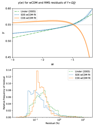
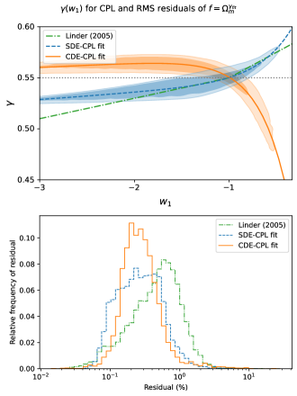
Figure 7: Different fits of $\gamma(w_{1})$ for $w$CDM models (left panels) and for CPL models (right panels) with contours for $\gamma(w_{1})$ for SDE (blue) and CDE (orange) in the the upper panels. The lower panels show histograms, normalized by relative frequency, of the RMS percent residual between the $\gamma$ given by fitting functions and the corresponding numerical value, obtained from the parametrization $f=\Omega_{m}^{\gamma}$.

Table 3: Coefficients for the fits of $\gamma(w_{1})=aw_{1}+be^{cw_{1}}+d$ for each collapse model and cosmology.

Model	Cosmology	$a$	$b$	$c$	$d$
SDE	$w$CDM	$0.0101$	$0.1266$	$2.8013$	$0.5532$
SDE	CPL	$0.0068$	$0.1346$	$2.8453$	$0.5493$
CDE	$w$CDM	$0.0047$	$-0.6320$	$3.8570$	$0.5706$
CDE	CPL	$0.0045$	$-0.4673$	$3.2250$	$0.5738$

The quality of the fits are demonstrated in the upper panels of Fig. 7, where our fits are well contained within the posteriors contours. The lower panels show the residuals of the parametrization of Eq. (3) and ours. We computed these residuals with the same RMS definition used for Fig. 4.

Let us first analyze the results for SDE in Fig. 4. Our fit is most accurate for the $w$CDM model (left panels), presenting a mode of residuals at $0.1\%$, while the linear fit of Eq. (3) presents a mode around $0.25\%$. In any case, very few realizations have with residuals $>1\%$. For the CPL models (right panels), our fit is noticeable better than the one of Eq. (3). For instance, the linear fit residuals, Eq. (3), peaks around $1\%$ while the exponential fit, Eq. (17), peaks at $0.2\%$. The main reason for this improvement is that the linear fit does not perform well for $w_{1}<-2$, as can be seen in the top panels of Fig. 4.

Our fitting function for $\gamma$ can also be used to describe the values for the CDE case, which are shown with orange lines and contours in Fig. 4. As can be seen, it also performs very well in models with clustering DE. The modes of the RMS residuals is around $0.1\%$ for both $w=\text{const.}$ and CPL parametrizations.

As an example of the use of our fit, in Tab. 4, we present the $\gamma$ values associated with the best-fit parameters obtained by DESI-BAO analysis [40]. As expected from the analysis already presented here, neither SDE nor CDE models are able to produce a high $\gamma$ value, but note that CDE can provide a slightly higher $\gamma$ because the $w_{0}w_{a}$ values have a phantom behavior at high an intermediate $z$. It is interesting to note that all these three DESI data analysis provide $w_{1}\simeq-1.2$, thus the $\gamma$ values for SDE or CDE are quite similar.

Table 4: Values of $\gamma$, given by Eq. (17), for DESI best-fit values for CPL parametrization using three different data combinations described in Ref. [40].

	$w_{0}$	$w_{a}$	$\gamma$-SDE	$\gamma$-CDE
DESI+CMB+Pahnth.	-0.872	-0.75	0.546	0.559
DESI+CMB+Union3	-0.65	-1.27	0.544	0.561
DESI+CMB+DESY5	-0.727	-1.05	0.545	0.560

V Conclusions

In this paper, we have analyzed the possibilities of DE models described by the CPL parametrization of producing a high value of $\gamma$, compatible with $\gamma=0.633^{+0.025}_{-0.024}$ obtained in Ref. [1]. As summarized in Fig. 6, both smooth DE and clustering DE have $\gamma$ distributions with small or negligible overlap with the $2\sigma$ interval of the measurement. This result depends only on the following assumptions: (1) $H\left(z\right)$ must be compatible with CC data, (2) $\Omega_{de}\left(z=1000\right)<0.01$ and (3) the priors described in Tab. 1. The combination of these assumptions imposes very loose constraints on $w_{0}w_{a}$ parameters, allowing for a vast, but meaningful, exploration of the possible values of $\gamma$.

We have also analyzed the correlations between $\gamma$, the EoS parameters and the clustering properties of DE. In particular, we can expect that phantom CDE models can raise the value of $\gamma$. However, since the impact of such models depend on $\Omega_{de}\left(z\right)\delta_{de}$, the actual change is very limited because $\Omega_{de}\left(z\right)$ decays rapidly with $z$. Non-phantom SDE can also give higher $\gamma$, but these realizations are correlated with very low $\Omega_{m0}\simeq 0.1$.

We have also proposed a new fitting function for $\gamma=\gamma(w_{1})$, with overall accuracies better than the linear fit of Eq. (3) covering the interval of $-3\leq w_{1}\leq-1/3$ . For the first time, we produced a $\gamma$ fitting function for CDE models, Eq. (17) with coefficients given in Tab. 3. These fits can be useful for a fast estimation of $\gamma$ for both SDE and CDE models described by CPL parametrization.

If the high $\gamma$ value found in Ref. [1] is validated by other observations and analysis, it poses a significant challenge to DE models based on minimally coupled scalar fields that can be described by the CPL EoS and a constant $c_{s}$ on small scales. Since we have considered the two limiting cases of smooth DE ($c_{s}=1$) and full clustering DE ($c_{s}=0$), it seems unlikely that intermediate or time-varying $c_{s}$ values can produce a significantly higher $\gamma$. A possible alternative is to consider more general EoS parametrizations. However, as demonstrated in our study, large variations on the EoS parameters and $\Omega_{m0}$ produce much narrower $\gamma$ distributions. Therefore, in principle, even more general EoS parametrizations should have some difficulties in explaining such high $\gamma$ values, with the disadvantage of introducing more parameters. If this ‘$\gamma$ tension’ persists, we might be seeing an early evidence of modified gravity or non-standard DM.