Impact of Charge on the Stability of Pulsar SAX J1748.9-2021 in Modified Symmetric Teleparallel Gravity

Abstract

In this paper, we explore the effect of charge on the stability of pulsar star SAX J1748.9-2021 in $f(Q)$ gravity, where $Q$ represents non-metricity. For this purpose, we apply the Krori-Barua metric ansatz with anisotropic fluid and use a linear $f(Q)$ model $f(Q)=\zeta Q$, where $\zeta$ is a non-zero constant. We derive exact relativistic solutions of the corresponding field equations. Furthermore, we study its geometric and physical properties through astrophysical observations from the pulsar SAX J1748.9-2021, which is found in X-ray binary systems within globular clusters. We examine features like anisotropic pressure, the mass-radius relationship, redshift, the Zeldovich condition, energy and causality conditions, the adiabatic index, the Tolman-Oppenheimer-Volkoff equation, the equation of state parameter and compactness. Our findings align with the observational data which indicate that the pulsar SAX J1748.9-2021 is viable and stable under this modified theory of gravity.

Keywords: Stellar configurations; Pulsar; $f(Q)$ gravity.
PACS: 97.10.-q; 97.60.Gb; 04.50.Kd.

1 Introduction

In the early 20th century, Albert Einstein introduced the general theory of relativity (GR), which revolutionized our understanding of the cosmos. This theory has been supported by numerous accurate observations, helping us to uncover many hidden aspects of the cosmos in modern cosmology. Subsequent observations of supernovae have confirmed that our universe is presently experiencing a rapid expansion phase [1]. There is a substantial evidence indicating that our universe is largely influenced by the mysterious components known as dark matter and dark energy (DE). Identifying the unknown form of energy is a challenging task for modern researchers. In GR, the cosmological constant $\Lambda$ is the simplest way to explain vacuum energy [2]. However, this approach has its limitations, as it cannot solve issues like fine-tuning [3] and coincidence problems [4]. In this context, it is believed that GR might not be the best model for describing gravity on large scales. Despite limited progress in understanding cosmic acceleration, research into modified theory of gravity (MTG) remains essential. These studies provide strong and logical alternatives to GR and might solve some current issues. Over the past two decades, numerous studies have been conducted on MTGs to explore and better understand the structure of the cosmos [5].

General relativity describes gravitational interactions using the Levi-Civita connection in Riemannian spacetime. This approach relies on the assumption of a geometry which is free from torsion and non-metricity. Additionally, it is important to remember that the general affine connection can be expressed more broadly [6]. Teleparallel gravity is an alternative theory to GR that explains gravitational interactions and is characterized by torsion $T$ [7]. Its teleparallel equivalent of GR (TEGR) uses the Weitzenb$\ddot{o}$ck connection, which means there is zero curvature and non-metricity involved [8]. In a cosmological model within Weyl-Cartan spacetime, the Weitzenb$\ddot{o}$ck connection involves the concept that the sum of the curvature and the scalar torsion vanishes [9]. The Riemann-Cartan spacetime is similar to the TEGR when the non-metricity is zero.

Symmetric teleparallel gravity is another alternative theory that assumes zero curvature and torsion while including non-metricity $Q$ [10]. The extension of these concepts leads us to $f(Q)$ gravity [11]. This theory has gained attention in research [12], exploring various geometric and physical implications, providing a new perspective on gravity and cosmic phenomena. Lazkoz et al. [13] examined the constraints of $f(Q)$ gravity using polynomial expressions related to redshift and analyzed energy conditions for two distinct models within this framework. Shekh [14] performed a dynamic analysis of the holographic DE model in the same gravity. Frusciante [15] proposed a model of this gravity that shares foundational similarities with the standard $\Lambda$ CDM model. In recent papers [16], we have constructed the generalized ghost DE and generalized ghost pilgrim DE models in $f(Q)$ using the correspondence principle within a non-interacting framework. We have also studied the pilgrim and generalized ghost pilgrim DE models for the non-interacting case [17]. These models reproduce different cosmic epochs, exploring a phantom phase of the universe and are consistent with the latest observational data.

Research on stellar structures within MTGs has gained significant attention over the past few decades. Pulsar SAX J1748.9-2021 (PS) is a neutron star located in our galaxy, known for its rapid rotation and strong magnetic field. Discovered in 1998 by the BeppoSAX/WFC satellite [18], it has emitted beams of radiation that create detectable pulses as it spins. Since its discovery, PS has experienced four outbursts, occurring approximately every five years [19], with the last one in 2015 [20]. These events help scientists to study the pulsar’s behavior and the extreme conditions present in neutron stars. An interesting aspect of PS is its role in an X-ray binary system, where it is paired with a companion star. Observations of these X-rays provide valuable information about the pulsar mass and structure. Research on PS enhances our understanding of neutron stars and the fundamental physics that govern these intriguing celestial objects [21].

Pulsars might not have a direct impact on cosmology, but they are very important for studying gravitational waves, researching dark matter, measuring cosmic distances accurately and other areas of precision astronomy. They are especially important for testing MTGs. Kramer et al. [22] studied the double pulsar system PSR J0737-3039A/B and highlighted its exceptional potential for conducting precise tests of GR and alternative theories. Its unique characteristics and proximity suggest that it could provide more accurate tests than current solar system experiments and may challenge existing assumptions about pulsar formation. Nashed [23] studied matter and geometry coupling in millisecond pulsars in $f(\mathcal{R},\mathbb{T})$ theory ($\mathcal{R},\mathbb{T}$ denote as Ricci scalar and trace of energy momentum tensor (EMT), respectively). They found that matter-geometry interactions lead to smaller star sizes as compared to GR and observations of 22 pulsars supported this theory, which fits well with linear trends and allows for neutron star mass up to 3.35 times the Sun mass. Recent studies have explored the effects of $f(\mathcal{R})$ and $f(\mathcal{R},\mathbb{T})$ gravity theories on PS in X-ray binary systems [24].

Maurya and Gupta [25] extended their model to derive solutions for an anisotropic charged fluid distribution, demonstrating that anisotropy and electric intensity increase from the core to the surface. Sharif and Waseem [26] examined the effects of charge on anisotropic relativistic compact star candidates within the $f(\mathcal{R},\mathbb{T})$ gravity. Using data from Her X-1, 4U1820-30 and SAX J 1808.4-3658, they explored physical properties and assessed stability, concluding that charge enhances stability. Sharif and Gul [27] explored the properties of charged compact stars with anisotropic matter using the embedding class-1 technique in $f(\mathcal{R},\mathbb{T}^{2})$ theory. Bhattacharjeea and Chattopadhyaya [28] explored spherically symmetric, anisotropic charged compact stars within the $f(Q)$ gravity framework, using the Krori-Barua metric and a linear $f(Q)$ model. They found that the charge intensity affects the star mass and radius and the model satisfies all stability as well as physical criteria, aligning with observational data.

This paper explores the impact of charge on the viable features and stability of anisotropic PS within the context of $f(Q)$ gravity. The structure of the paper is as follows. Section 2 explains the fundamentals of $f(Q)$ gravity and its field equations with charge. It also covers how the Einstein-Maxwell equations are formulated and solved within this theory. In section 3, we present the field equations for a specific $f(Q)$ model and apply the KB ansatz. Matching conditions are used to determine the unknown constants in the KB ansatz. Sections 4 and 5 utilize observational data from PS to derive density, radial and tangential pressures, anisotropy, the mass-radius relation, redshift, the Zeldovich condition, energy conditions, the causality condition, the adiabatic index, the Tolman-Oppenheimer-Volkoff (TOV) equation, the equation of state (EoS) parameter and compactness. We also evaluate the stability of the model based on these physical constraints. Finally, our conclusions are presented in section 6.

2 $f(Q)$ Gravity and the Einstein-Maxwell Equations

The action for $f(Q)$ gravity, which incorporates the matter Lagrangian $L_{m}$ and the Lagrangian of the electromagnetic field $L_{e}$, is expressed as follows [11]

$$S=\int\frac{1}{2}f(Q)\sqrt{-g}d^{4}x+\int(L_{m}+L_{e})\sqrt{-g}d^{4}x.$$ (1)

The Lagrangian for the electromagnetic field is given by

$$L_{e}=-\frac{1}{16\pi}F_{\alpha\beta}F^{\alpha\beta},$$ (2)

where $F_{\alpha\beta}=\varphi_{\alpha,\beta}-\varphi_{\beta,\alpha}$ represents the Maxwell field tensor and $\varphi_{\alpha}$ denotes the four-potential. The determinant of the metric tensor is defined as $g$, $L_{m}$ is the matter Lagrangian density. The non-metricity scalar is described as

$$Q=-g^{\mu\nu}(\mathbb{L}^{\varrho}_{~{}\phi\mu}\mathbb{L}^{\phi}_{~{}\nu\varrho}-\mathbb{L}^{\varrho}_{~{}\phi\varrho}\mathbb{L}^{\phi}_{~{}\mu\nu}),$$ (3)

where

$$\mathbb{L}^{\varrho}_{\;\phi\mu}=-\frac{1}{2}g^{\varrho\lambda}(\nabla_{\mu}g_{\phi\lambda}+\nabla_{\phi}g_{\lambda\mu}-\nabla_{\lambda}g_{\phi\mu}).$$ (4)

The superpotential is characterized as

$$\mathbb{P}^{\varrho}_{\;\mu\nu}=-\frac{1}{2}\mathbb{L}^{\varrho}_{\;\mu\nu}+\frac{1}{4}(Q^{\varrho}-\tilde{Q}^{\varrho})g_{\;\mu\nu}-\frac{1}{4}\delta^{\varrho}\;_{({\mu}}Q_{\nu)},$$ (5)

where $Q_{\varrho}=Q^{~{}\mu}_{\varrho~{}\mu}$ and $\tilde{Q}_{\varrho}=Q^{\mu}_{~{}\varrho\mu}$. Thus, the expression for $Q$ becomes [29]

$$Q=-Q_{\varrho\zeta\tau}\mathbb{P}^{\varrho\zeta\tau}=-\frac{1}{4}(-Q^{\varrho\tau\rho}Q_{\varrho\tau\rho}+2Q^{\varrho\tau\rho}Q_{\rho\varrho\tau}-2Q^{\rho}\tilde{Q}_{\rho}+Q^{\rho}Q_{\rho}).$$ (6)

The field equations associated with $f(Q)$ gravity can be written as

$$\frac{-2}{\sqrt{-g}}\nabla_{\varrho}(f_{Q}\sqrt{-g}P^{\varrho}_{~{}\mu\nu})-\frac{1}{2}fg_{\mu\nu}-f_{Q}(P_{\mu\varrho\phi}Q_{\nu}^{~{}\varrho\phi}-2Q^{\varrho\phi}_{~{}~{}~{}\mu}P_{\varrho\phi\nu})=\mathbb{T}_{\mu\nu}+E_{\mu\nu},$$ (7)

here $f_{Q}$ represents the derivative with respect to $Q$.

The line element for a spherically symmetric spacetime is

$$ds^{2}=e^{\xi(r)}dr^{2}-e^{\psi(r)}dt^{2}+r^{2}(d\theta^{2}+\sin^{2}\theta d\phi^{2}).$$ (8)

An anisotropic perfect fluid is a type of fluid in which the pressure differs in different directions, unlike an isotropic perfect fluid where the pressure is same in all directions. The EMT for an anisotropic perfect fluid can be written as

$$\mathbb{T}_{\mu\nu}=(\rho+p_{t})u_{\mu}u_{\nu}+p_{t}g_{\mu\nu}-\chi k_{\mu}k_{\nu},$$ (9)

In this context, $\rho$ represents the energy density of the fluid, while $p_{r}$ is the radial pressure and $p_{t}$ is the tangential pressure. The four-velocity components of the fluid, denoted as $u_{\mu}$ and $u_{\nu}$, adhere to the normalization condition $u^{\mu}u_{\mu}=-1$. Additionally, $k_{\mu}$ is a unit four-vector in the radial direction, satisfying $k^{\mu}k_{\mu}=1$. The anisotropy factor $\chi$ is defined as the difference between the tangential pressure and the radial pressure, expressed as $\chi=p_{t}-p_{r}$. Using the provided metric, $u^{\mu}$ can be written as $e^{-\psi}\delta^{\mu}_{t}$ and $k^{\mu}$ as $e^{-\xi}\delta^{\mu}_{r}$. As a result, the trace of the EMT (9) can be written as

$$\mathbb{T}=-\rho+3p_{r}+2\chi.$$ (10)

The stress-energy tensor for the electromagnetic field is expressed by

$$E_{\mu\nu}=\frac{1}{4\pi}\bigg{(}F^{\beta}_{\mu}F_{\nu\beta}-\frac{1}{4}g_{\mu\nu}F_{\alpha\beta}F^{\alpha\beta}\bigg{)}.$$ (11)

The corresponding Maxwell equations are

$$(\sqrt{-g}F_{\mu\nu})_{;\nu}=4\pi J_{\mu}\sqrt{-g},\quad F_{[\mu\nu;\delta]}=0.$$ (12)

In this context, it specifically refers to the covariant derivative with respect to the Levi-Civita connection, which is the standard connection used in GR for ensuring that the covariant derivative is compatible with the metric and has no torsion. Where $J_{\mu}=\sigma u_{\mu}$ represents the electric four-current, $\sigma$ is the charge density. The electric field strength $E(r)$ is expressed as

$$E(r)=\frac{e^{\frac{\psi+\xi}{2}}}{r^{2}}q(r),$$ (13)

where $q(r)$ represents the total charge enclosed within a sphere of radius $r$, calculated as

$$q(r)=4\pi\int_{0}^{r}\sigma r^{2}e^{\xi}dr,$$ (14)

leading to

$$\sigma=\frac{e^{-\xi}}{4\pi r^{2}}\frac{dq(r)}{dr}.$$ (15)

In this study, we use a specific charge distribution given by [30]

$$q=q_{0}r^{3},$$ (16)

where $q_{0}$ represents the charge intensity. If $q_{0}=0$, it corresponds to a neutral, uncharged scenario. The field equations (7) have the following non-zero components

$$\rho = \frac{1}{2r^{2}e^{\xi}}\bigg{[}f_{Q}\bigg{(}\big{(}e^{\xi}-1\big{)}\big{(}r\psi^{\prime}+2\big{)}+r\big{(}e^{\xi}+1\big{)}\xi^{\prime}\bigg{)}$$ (17)

$$+ 2rf_{QQ}\big{(}e^{\xi}-1\big{)}Q^{\prime}+fr^{2}e^{\xi}\bigg{]}-\frac{(q_{0}r^{3})^{2}}{r^{4}},$$

$$p_{r} = \frac{1}{2r^{2}e^{\xi}}\bigg{[}f_{Q}\bigg{(}\big{(}e^{\xi}-1\big{)}\big{(}r\psi^{\prime}+r\xi^{\prime}+2\big{)}-2r\psi^{\prime}\bigg{)}$$ (18)

$$+ 2f_{QQ}r\big{(}e^{\xi}-1\big{)}Q^{\prime}+fr^{2}e^{\xi}\bigg{]}+\frac{(q_{0}r^{3})^{2}}{r^{4}},$$

$$p_{t} = \frac{-1}{4re^{\xi}}\bigg{[}f_{Q}\big{(}\xi^{\prime}\big{(}r\psi^{\prime}+2e^{\xi}\big{)}-r\psi^{\prime 2}-2\psi^{\prime\prime}r+2\big{(}e^{\xi}-2\big{)}\psi^{\prime}\big{)}$$ (19)

$$- 2f_{QQ}rQ^{\prime}\psi^{\prime}+2fre^{\xi}\bigg{]}-\frac{(q_{0}r^{3})^{2}}{r^{4}},$$

where prime is the derivative with respect to $r$. The non-metricity scalar can be given as

$$Q=\frac{e^{-\xi}\big{(}1-e^{\xi}\big{)}\big{(}\psi^{\prime}+\xi^{\prime}\big{)}}{r}.$$ (20)

3 The $f(Q)$ Gravity Model

The most widely recognized initial model of $f(Q)$ theory is the linear model [31]

$$f(Q)=\zeta Q,$$ (21)

where $\zeta$ is an arbitrary constant and it is not fixed like gravitational constant $G$ but is instead varied using a hit and trail approach to optimize the model for different cosmic behaviors. Thus, it allows flexibility in matching the model to observational data by adjusting the parameter to find the best-fit behavior of key cosmic parameters like expansion rates or DE contributions. As this constant is determined theoretically, it differs from the $G$ in terms of its role in the theory. While $G$ is universally defined across all gravitational phenomena, the modified gravitational coupling in this model is treated more as a tunable parameter to accommodate specific cosmic observations. Therefore, the comparison between the two is limited, as the arbitrary constant does not universally define gravitational strength but is used to explore how varying this constant affects the behavior of the STEGR model, especially in regimes where deviations from GR are expected. In particular, the linear model clarifies that when $\zeta=1$, the model reduces to STEGR, fully recovering the gravitational dynamics of GR. Here $f_{Q}=\zeta$ and $f_{QQ}=0$. We substitute these values into Eqs.(17)-(19) and obtain

$$\rho = \frac{-q^{2}+\zeta r^{2}e^{-\xi(r)}\bigg{(}r\xi^{\prime}-1\bigg{)}+\zeta r^{2}}{r^{4}},$$ (22)

$$p_{r} = \frac{1}{2r^{2}}\bigg{[}\big{(}2r^{3}e^{2\xi}\big{(}-\zeta\big{(}\psi^{\prime}+\xi^{\prime}\big{)}\big{)}+\zeta e^{\xi}\big{(}r\big{(}2r^{2}+1\big{)}\big{(}\psi^{\prime}+\xi^{\prime}\big{)}+2\big{)}$$ (23)

$$- \zeta\big{(}3r\psi^{\prime}+r\xi^{\prime}+2\big{)}\big{)}e^{-\xi}\bigg{]}+\frac{q^{2}}{r^{4}},$$

$$p_{t} = \frac{1}{4}\bigg{[}\frac{1}{r}\bigg{\{}\zeta e^{-\xi}\bigg{(}r\psi^{\prime 2}-2\xi^{\prime}+2r\psi^{\prime\prime}+\psi^{\prime}\big{(}2-r\xi^{\prime}\big{)}\bigg{)}\bigg{\}}\bigg{]}-\frac{q^{2}}{r^{4}},$$ (24)

To understand how stars evolve, we make some reasonable assumptions about two key functions $\xi(r)$ and $\psi(r)$.

3.1 The Krori-Barua Spacetime

The KB scheme is a set of metric potentials used to model compact objects in GR as well as in various MTGs. This scheme provides a framework for describing the gravitational field within a spherically symmetric star [32]. The metric potentials in the KB spacetime are expressed as

$$\psi(r)=\eta_{0}r^{2}+\eta_{1},~{}~{}~{}\xi(r)=\eta_{2}r^{2},$$ (25)

where $\eta_{0},\eta_{1},\eta_{2}$ are arbitrary constants determined by junction conditions. This solution ensures that the interior of the star is smooth and free of singularities.

3.2 Matching Conditions

In a stellar system, we can assume that solutions from non-Riemannian geometry in a vacuum are the same as those from $f(Q)$ theory. This means that the model described by (21) applies here as well. As a result, the external solution aligns with the vacuum charged exterior Reissner-Nordstr$\ddot{o}$m (RN) solution. Therefore, we use the following model to describe the exterior spacetime as

$$ds^{2}=-\bigg{(}1+\frac{\mathbb{Q}^{2}}{r^{2}}-\frac{2\mathbb{M}}{r}\bigg{)}dt^{2}+\bigg{(}1+\frac{\mathbb{Q}^{2}}{r^{2}}-\frac{2\mathbb{M}}{r}\bigg{)}^{-1}dr^{2}+r^{2}(d\theta^{2}+\sin^{2}\theta d\phi^{2}).$$ (26)

Here $\mathbb{M}$ denotes the gravitational mass of the star. Ensuring that the metric coefficients from (8), (25) and (26) are continuous at the boundary surface ($r=\mathbb{R}$) leads to the geometric component given by

$$g_{tt} = e^{\eta_{0}\mathbb{R}^{2}+\eta_{1}}=\bigg{(}1+\frac{\mathbb{Q}^{2}}{\mathbb{R}^{2}}-\frac{2\mathbb{M}}{\mathbb{R}}\bigg{)},$$ (27)

$$g_{rr} = e^{\eta_{2}\mathbb{R}^{2}}=\bigg{(}1+\frac{\mathbb{Q}^{2}}{\mathbb{R}^{2}}-\frac{2\mathbb{M}}{\mathbb{R}}\bigg{)}^{-1},$$ (28)

$$g_{tt,r} = 2\eta_{0}\mathbb{R}e^{\eta_{0}\mathbb{R}^{2}+\eta_{1}}=\frac{2\mathbb{M}}{\mathbb{R}^{2}}-\frac{2\mathbb{Q}^{2}}{\mathbb{R}^{3}}.$$ (29)

Solving (27)-(29) and applying the condition $p_{r}(r=\mathbb{R})=0$, the constants $\eta_{0}$, $\eta_{1}$ and $\eta_{2}$ can be found as follows

$$\eta_{0} = \bigg{(}-\frac{2\mathbb{Q}^{2}}{\mathbb{R}^{4}}+\frac{2\mathbb{M}}{\mathbb{R}^{3}}\bigg{)}\bigg{(}-\frac{2\mathbb{M}}{\mathbb{R}}+1+\frac{\mathbb{Q}^{2}}{\mathbb{R}^{2}}\bigg{)}^{-1},$$ (30)

$$\eta_{1} = \ln\bigg{(}1-\frac{2\mathbb{M}}{\mathbb{R}}+\frac{\mathbb{Q}^{2}}{\mathbb{R}^{2}}\bigg{)}-\bigg{(}\frac{2\mathbb{M}}{\mathbb{R}^{3}}-\frac{2\mathbb{Q}^{2}}{\mathbb{R}^{4}}\bigg{)}\bigg{(}1-\frac{2\mathbb{M}}{R}+\frac{\mathbb{Q}^{2}}{\mathbb{R}^{2}}\bigg{)}^{-1},$$ (31)

$$\eta_{2} = \frac{\ln\bigg{(}\frac{\mathbb{R}^{2}}{-2\mathbb{M}\mathbb{R}+\mathbb{Q}^{2}+\mathbb{R}^{2}}\bigg{)}}{\mathbb{R}^{2}}.$$ (32)

4 Stability Analysis from SAX J1748.9-2021 Observations

In this section, we utilize observational data, specifically the mass and radius of the PS within the $f(Q)$ gravity. We examine the stability of the solution to be obtained by applying various constraints. Accurate observational data is essential for determining the model parameters. We rely on detailed spectroscopic data from EXO 1745-248 during thermonuclear bursts, which has given precise measurements for the pulsar mass ($\mathbb{M}=1.81\pm 0.3\mathbb{M}_{\odot}$) and radius ($\mathbb{R}=11.7\pm 1.7km$) [33]. Using these measurements, we explore physical characteristics and stability of the pulsar.

4.1 The Material Component

Substituting Eq.(25) into (22)-(24), we can derive the expressions for $\rho$, $p_{r}$ and $p_{t}$ as follows

$$\rho = \frac{\zeta e^{-(\eta_{2}r^{2})}\bigg{(}2\eta_{2}r^{2}-1\bigg{)}+\zeta-q_{0}^{2}r^{4}}{r^{2}},$$ (33)

$$p_{r} = \frac{1}{r^{2}}\bigg{[}e^{-\eta_{2}r^{2}}\bigg{(}e^{\eta_{2}r^{2}}\bigg{(}\zeta\big{(}\big{(}2r^{2}+1\big{)}r^{2}(\eta_{0}+\eta_{2})\big{)}+q_{0}^{2}r^{4}\bigg{)}$$

$$- \zeta\big{(}r^{2}(3\eta_{0}+\eta_{2})\big{)}-2\zeta r^{4}(\eta_{0}+\eta_{2})e^{2\eta_{2}r^{2}}\bigg{)}\bigg{]},$$

$$p_{t} = \zeta e^{-\eta_{2}r^{2}}\bigg{(}\eta_{0}r^{2}(\eta_{0}-\eta_{2})(2\eta_{0}-\eta_{2})\bigg{)}-q_{0}^{2}r^{2}.$$ (34)

We create plots of $\rho$, $p_{r}$ and $p_{t}$ against the radial distance. For our analysis, we have used the values $\eta_{0}=0.00363$, $\eta_{1}=-0.40562$ and $\eta_{2}=0.00405$. We choose $Q=3$ because it gibes better results in the graphs. Additionally, we vary the value of $q_{0}$ as $0.004$, $0.006$ and $0.008$ for our graphical analysis. Higher $q_{0}$ increases repulsion from the electric field, which affects the gravitational potential and makes the charge’s effect more visible. In $f(Q)$ theory, smaller charges result in fewer changes in the gravitational field, whereas larger charges lead to stronger electric repulsion. The plots of $\rho$, $p_{r}$ and $p_{t}$ are shown in Figure 1. These values are highest at the center of the star and gradually decrease as we move outward. This shows that the matter is very dense at the center and becomes less dense towards the edge, indicating a highly concentrated profile of the PS with increasing $r$.

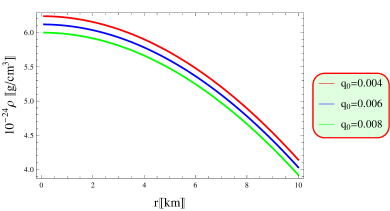
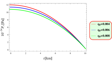
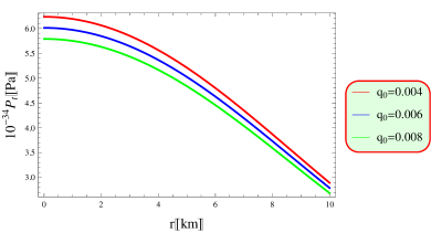
Figure 1: Graphs of $\rho$, $p_{r}$, $p_{t}$ as functions of $r$.

Anisotropic pressure refers to the condition where the pressure inside a star or similar object varies in different directions. This can happen because of quantities like strong magnetic fields, the star rotation or different types of matter inside the star. This variation in pressure can have a big impact on the stability and structure of compact objects like PS [34]. It is expressed as

$$\chi = \frac{1}{r^{2}}\bigg{[}e^{-\eta_{2}r^{2}}\bigg{(}\zeta\big{(}\eta_{0}\eta_{2}r^{4}-\eta_{0}^{2}r^{4}-5\eta_{0}r^{2}\big{)}+e^{\eta_{2}r^{2}}\bigg{(}2q_{0}^{2}r^{4}+\zeta\big{(}2\eta_{0}r^{4}$$

$$+ \eta_{0}r^{2}+2\eta_{2}r^{4}+\eta_{2}r^{2}\big{)}\bigg{)}-2\zeta r^{4}(\eta_{0}+\eta_{2})e^{2\eta_{2}r^{2}}\bigg{)}\bigg{]}.$$

Figure 2 demonstrates that the anisotropy meets the stability criteria. It begins from zero at the center of the star and gradually increases in a consistent manner towards the star’s surface.

Providing numerical values for the physical properties of the pulsar as predicted by the current model, is crucial. For example, when $q_{0}$ is 0.004, $\rho_{core}\approx 6.24\times 10^{16}$ g/cm³, $p_{r(core)}\approx 11.95\times 10^{34}$ dyn/cm² and $p_{t(core)}\approx 6.24\times 10^{34}$ dyn/cm². At the star’s surface, $\rho_{I}\approx 4.14\times 10^{16}$ g/cm³ with $p_{r(r=\mathbb{R})}=0$ dyn/cm² and $p_{t(r=\mathbb{R})}\approx 2.89\times 10^{34}$ dyn/cm². For $q_{0}=0.006$, $\rho_{core}\approx 6.12\times 10^{16}$ g/cm³, $p_{r(core)}\approx 11.31\times 10^{34}$ dyn/cm² and $p_{t(core)}\approx 5.99\times 10^{34}$ dyn/cm². At the star’s surface, $\rho_{I}\approx 4.06\times 10^{16}$ g/cm³ with $p_{r(r=\mathbb{R})}=0$ dyn/cm² and $p_{t(r=\mathbb{R})}\approx 2.78\times 10^{34}$ dyn/cm². When $q_{0}=0.008$, $\rho_{core}\approx 5.98\times 10^{16}$ g/cm³, $p_{r(core)}\approx 10.79\times 10^{34}$ dyn/cm² and $p_{t(core)}\approx 5.79\times 10^{34}$ dyn/cm². At the star’s surface, $\rho_{I}\approx 3.94\times 10^{16}$ g/cm³ with $p_{r(r=\mathbb{R})}=0$ dyn/cm² and $p_{t(r=\mathbb{R})}\approx 2.68\times 10^{34}$ dyn/cm².

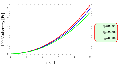
Figure 2: Graphical representation of $\chi$ relative to $r$.

4.2 Limit on the Mass-Radius Relation

The mass of PS is given as [33]

$$M(r)=4\pi\int_{0}^{r}\gamma^{2}\rho(\gamma)d\gamma.$$

Using Eq.(33) and performing the integration, we obtain

$$M(r)=4\pi\bigg{(}\zeta r\bigg{(}1-e^{-\eta_{2}r^{2}}\bigg{)}-\frac{q_{0}^{2}r^{5}}{5}\bigg{)}.$$ (35)

This numerical analysis evaluates the reliability of the current model, as depicted in Figure 3. The mass function rises steadily and evenly as the star’s radius increases.

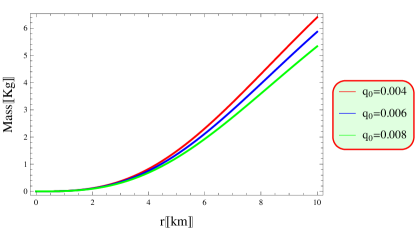
Figure 3: Graph of mass-radius as functions of $r$.

4.3 The Gravitational Redshift

This is the effect where light or electromagnetic radiation shifts to longer wavelengths as it escapes from a strong gravitational field. This occurs because the energy of the photons decreases in the gravitational potential of a massive object. The stronger the gravitational field, such as near a black hole or a dense star, the more significant the redshift. This phenomenon, predicted by GR, helps us to understand the influence of gravity on light and can be observed in the spectra of stars and other celestial objects. Ivanov [35] calculated the value to be 5.211 for anisotropic configurations that adhere to the dominant energy condition. The gravitational redshift function is given by

$$Z(r)=\frac{1}{\sqrt{1-\varpi}}-1,$$

where $\varpi=\frac{2M}{r}$. Applying Eq.(35), we obtain

$$Z(r)=\frac{1}{\sqrt{8\pi\zeta\bigg{(}e^{-\eta_{2}r^{2}}-1\bigg{)}+\frac{8}{5}\pi q_{0}^{2}r^{4}+1}}-1.$$ (36)

We create a graph of the redshift function for the pulsar using different values of $q_{0}$. The gravitational redshift stays positive and finite inside the star and gradually increases, as shown in Figure 4 [36]. The redshift function stays within the specified limit ($Z(r)<5.211$).

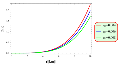
Figure 4: Graph of redshift as functions of $r$.

4.4 The Zeldovich Condition

The Zeldovich condition [37] is a key criterion in astrophysics for evaluating the stability of stars, particularly within the frameworks of GR and stellar astrophysics. According to the Zeldovich condition, the ratio of the central pressure $p(0)$ to the central energy density $\rho(0)$ must satisfy specific requirements to ensure the stability of the star. This condition helps in understanding the balance between gravitational forces and the internal pressure that prevents collapse. It is defined as

$$\frac{p(0)}{c^{2}\rho(0)}\leq 1.$$ (37)

We should verify that this ratio does not exceed 1. The values of $\rho$, $p_{r}$ and $p_{t}$ when $r\rightarrow 0$ can be determined as follows

$$\rho(0)=2\eta_{2}\zeta,\quad p_{r}(0)=\zeta(-2\eta_{0}+\eta_{2}),\quad p_{t}(0)=(2\eta_{0}-\eta_{2})\zeta.$$

Using the values previously calculated for the PS in section 4.1, we can assess Zeldovich’s inequality (37). According to the expressions above, the ratio $\frac{p_{r}(0)}{\rho(0)}$ is 0.7, which is less than 1. Similarly, the ratio $\frac{p_{t}(0)}{\rho(0)}$ is -1.1, also less than 1. These results show that the Zeldovich condition is satisfied in both cases.

4.5 Energy Conditions

Energy conditions are important criteria in GR and cosmology, used to constrain the behavior of matter and energy in spacetime. They help to ensure that the EMT behaves in a physically reasonable way. There are several types of energy conditions

1. Null energy condition is represented as

   $0\leq\rho+p_{r},\quad 0\leq\rho+p_{t}$.

2. Dominant energy condition is expressed as

   $0\leq\rho-p_{r},\quad 0\leq\rho-p_{t}$.

3. Weak energy condition is presented as

   $0\leq\rho+p_{r},\quad 0\leq\rho+p_{t},\quad 0\leq\rho$.

4. Strong energy condition is stated as

   $0\leq\rho+p_{r},\quad 0\leq\rho+p_{t},\quad 0\leq\rho+p_{r}+2p_{t}$.

These conditions are crucial in understanding how cosmic structures form and stay stable within spacetime. They help to determine if a PS can exist and remain stable. Figure 5 shows the energy conditions for different values of $q_{0}$ and demonstrates that the PS meets all the necessary energy conditions.

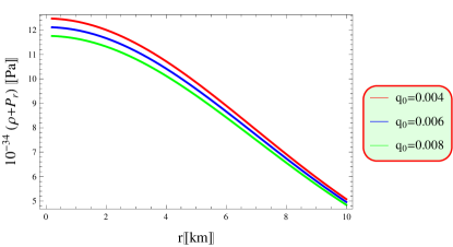
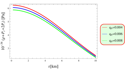
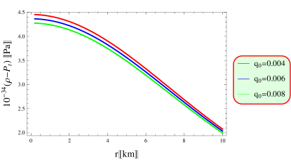
Figure 5: Graphical representations of energy conditions relative to $r$.

4.6 Causality Conditions

In cosmology, these conditions ensure that nothing exceeds the speed of light. For an anisotropic fluid, it is defined as

$$v_{r}^{2}=\frac{{p}_{r}^{\prime}}{\rho^{\prime}},\quad v_{t}^{2}=\frac{{p}_{t}^{\prime}}{\rho^{\prime}}.$$ (38)

For a neutron star like PS, the squared speed of sound must lie within a specific range $[0,1]$ to maintain structural stability [38]. The radial and tangential sound speeds both satisfy the stability criteria, which specify that $0\leq\frac{v_{r}^{2}}{c^{2}}\leq 1$ and $0\leq\frac{v_{t}^{2}}{c^{2}}\leq 1$. Additionally, stability is assessed using the cracking condition $0\leq\frac{v_{t}^{2}-v_{r}^{2}}{c^{2}}\leq 1$ [39]. If this condition is fulfilled, the PS remains stable and can persist for a long time, otherwise, it may collapse. Applying the equation provided, we obtain

$$v_{r}^{2} = \bigg{[}\zeta\big{(}2\eta_{2}^{2}r^{4}-\eta_{2}r^{2}\big{)}+e^{\eta_{2}r^{2}}\big{(}\zeta+q_{0}^{2}r^{4}\big{)}\bigg{]}\bigg{[}2\zeta r^{4}(\eta_{0}+\eta_{2})e^{2\eta_{2}r^{2}}\big{(}\eta_{2}r^{2}\big{)}-\zeta$$ (39)

$$\times \big{(}3\eta_{0}\eta_{2}r^{4}+\eta_{2}^{2}r^{4}+\eta_{2}r^{2}\big{)}-e^{\eta_{2}r^{2}}\bigg{(}q_{0}^{2}r^{4}+\zeta\big{(}2\eta_{0}r^{4}+2\eta_{2}r^{4}\big{)}\bigg{)}\bigg{]}^{-1},$$

$$v_{t}^{2} = \bigg{[}\zeta\big{(}-2\eta_{2}^{2}r^{4}+\eta_{2}r^{2}\big{)}-e^{\eta_{2}r^{2}}\big{(}\zeta+q_{0}^{2}r^{4}\big{)}\bigg{]}\bigg{[}r^{4}\bigg{(}\zeta\big{(}\eta_{2}^{2}+\eta_{0}\eta_{2}\big{(}\eta_{2}r^{2}-3\big{)}$$ (40)

$$+ \eta_{0}^{2}\big{(}-\eta_{2}r^{2}\big{)}\big{)}-q_{0}^{2}e^{\eta_{2}r^{2}}\bigg{)}\bigg{]}^{-1},$$

where

$$\rho^{\prime} = \frac{1}{r^{2}}\bigg{[}\big{(}4\eta_{2}\zeta re^{-\eta_{2}r^{2}}\big{)}-\bigg{(}2\eta_{2}\zeta re^{-\eta_{2}r^{2}}\bigg{(}2\eta_{2}r^{2}-1\bigg{)}\bigg{)}-4q_{0}^{2}r^{3}\bigg{]}-\frac{1}{r^{3}}$$

$$\times \bigg{[}2\bigg{(}\zeta e^{-\eta_{2}r^{2}}\bigg{(}2\eta_{2}r^{2}-1\bigg{)}+\zeta-q_{0}^{2}r^{4}\bigg{)}\bigg{]},$$

$$p_{r}^{\prime} = -\frac{1}{r}\bigg{[}2\eta_{2}e^{-\eta_{2}r^{2}}\bigg{(}e^{\eta_{2}r^{2}}\bigg{(}\zeta\big{(}\big{(}2r^{2}+1\big{)}r^{2}(\eta_{0}+\eta_{2})\big{)}+q_{0}^{2}r^{4}\bigg{)}-\zeta r^{2}(3\eta_{0}$$

$$+ \eta_{2})-2\zeta r^{4}(\eta_{0}+\eta_{2})e^{2\eta_{2}r^{2}}\bigg{)}\bigg{]}-\frac{1}{r^{3}}\bigg{[}2e^{-\eta_{2}r^{2}}\bigg{(}e^{\eta_{2}r^{2}}\big{(}\zeta\big{(}\big{(}2r^{2}+1\big{)}r^{2}(\eta_{0}$$

$$+ \eta_{2})\big{)}+q_{0}^{2}r^{4}\big{)}-\zeta\big{(}r^{2}(3\eta_{0}+\eta_{2})\big{)}-2\zeta r^{4}(\eta_{0}+\eta_{2})e^{2\eta_{2}r^{2}}\bigg{)}\bigg{]}+\frac{1}{r^{2}}\bigg{[}e^{-\eta_{2}r^{2}}$$

$$\times \bigg{(}\bigg{(}2\eta_{2}re^{\eta_{2}r^{2}}\bigg{(}q_{0}^{2}r^{4}+\zeta\big{(}\big{(}2r^{2}+1\big{)}r^{2}(\eta_{0}+\eta_{2})\big{)}\bigg{)}\bigg{)}+e^{\eta_{2}r^{2}}\bigg{(}\zeta\big{(}4r^{3}(\eta_{0}$$

$$+ \eta_{2})+2\big{(}2r^{2}+1\big{)}r(\eta_{0}+\eta_{2})\big{)}+4q_{0}^{2}r^{3}\bigg{)}-\bigg{(}8\eta_{2}\zeta r^{5}(\eta_{0}+\eta_{2})e^{2\eta_{2}r^{2}}\bigg{)}$$

$$- 8\zeta r^{3}(\eta_{0}+\eta_{2})e^{2\eta_{2}r^{2}}-2\zeta r(3\eta_{0}+\eta_{2})\bigg{)}\bigg{]},$$

$$p_{t}^{\prime} = \big{(}2\eta_{0}\zeta r(\eta_{0}-\eta_{2})e^{-\eta_{2}r^{2}}\big{)}-2q_{0}^{2}r\big{(}2\eta_{2}\zeta r\big{(}\eta_{0}r^{2}(\eta_{0}-\eta_{2})+(2\eta_{0}-\eta_{2})\big{)}e^{-\eta_{2}r^{2}}\big{)}.$$

Figure 6 depicts how the radial and tangential squared speed of sound vary with $r$. It shows that $v_{r}^{2}$ ranges from 0.785 to 0.793 and $v_{t}^{2}$ ranges from 0.832 to 0.849. Additionally, the difference $(v_{t}^{2}-v_{r}^{2})$ lies between 0.011 and 0.012 throughout the interior of the PS. These findings confirm that all the necessary stability conditions are fulfilled, ensuring the stability of the PS.

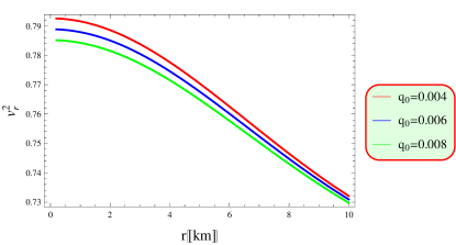
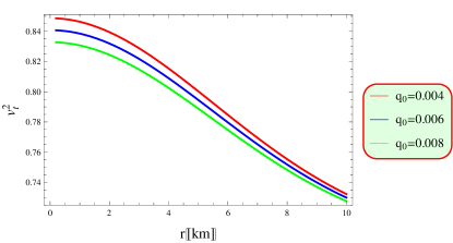
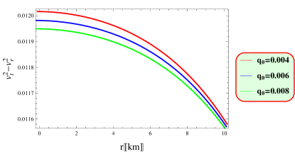
Figure 6: Graphs of causality condition as functions of $r$.

4.7 The Adiabatic Index and the Equilibrium of Hydrodynamic Forces

The adiabatic index $(\Gamma)$ is a crucial parameter for assessing the stability of stars, including PS. It provides insight into how pressure and density affect the star’s stability. It is defined by the formula [40]

$$\Gamma=\frac{4}{3}\bigg{(}\frac{\chi}{|p_{r}^{\prime}|r}+1\bigg{)}_{max}.$$

This expression helps to determine the star’s response towards the compression and expansion which is vital for understanding its structural integrity. For radial ($\Gamma_{r}$) and tangential ($\Gamma_{t}$) components, it is given by

$$\Gamma_{r}=\frac{\nu_{r}^{2}(p_{r}+\rho c^{2})}{p_{t}},\quad\Gamma_{t}=\frac{\nu_{t}^{2}(p_{t}+\rho c^{2})}{p_{t}}.$$

For stability, $\Gamma$ must be greater than $4/3$. In an isotropic system, where the pressure is the same in all directions $(\chi=0)$, the parameter $\Gamma$ equals $4/3$. In cases of mild anisotropy $(\chi<0)$, the $\Gamma$ remains greater $4/3$, which is consistent with the standard stability condition. In cases of strong anisotropy $(\chi>0)$, as explored in this study, the $\Gamma$ can be greater than $4/3$. Neutral equilibrium is achieved when the adiabatic indices for $\Gamma_{r}$ and $\Gamma_{t}$ are equal. For a star to maintain stable equilibrium, both $\Gamma_{r}$ and $\Gamma_{t}$, must be greater than the $\Gamma$. Specifically for a PS, stability is ensured if both $\Gamma_{r}$ and $\Gamma_{t}$ are greater than $4/3$. If these conditions are not satisfied, the star may become unstable and could potentially collapse [41]. Using the above equation, we find

$$\Gamma = -\bigg{[}2\zeta\bigg{(}\eta_{0}^{2}r^{4}-\eta_{0}r^{2}\bigg{(}\eta_{2}r^{2}\bigg{(}4r^{2}e^{2\eta_{2}r^{2}}-5\bigg{)}+\bigg{(}2r^{2}e^{2\eta_{2}r^{2}}+\big{(}1-2r^{2}\big{)}$$

$$\times e^{\eta_{2}r^{2}}-5\bigg{)}\bigg{)}+\eta_{2}^{2}\bigg{(}2r^{4}-4r^{6}e^{2\eta_{2}r^{2}}\bigg{)}-\eta_{2}r^{2}\bigg{(}2r^{2}e^{2\eta_{2}r^{2}}+\big{(}1-2r^{2}\big{)}$$

$$\times e^{\eta_{2}r^{2}}-2\bigg{)}-3\bigg{(}e^{\eta_{2}r^{2}}-1\bigg{)}\bigg{)}\bigg{]}\bigg{[}-\big{(}3\eta_{0}\eta_{2}r^{4}+\eta_{2}^{2}r^{4}+\eta_{2}r^{2}\big{)}3\zeta-3$$

$$\times e^{\eta_{2}r^{2}}\bigg{(}\zeta\big{(}2\eta_{0}r^{4}+2\eta_{2}r^{4}\big{)}+q_{0}^{2}r^{4}\bigg{)}+6\zeta r^{4}(\eta_{0}+\eta_{2})e^{2\eta_{2}r^{2}}\bigg{(}\eta_{2}r^{2}\bigg{)}\bigg{]}^{-1},$$

$$\Gamma_{r} = \bigg{[}\zeta\bigg{(}\eta_{0}r^{2}\bigg{(}2r^{2}e^{2\eta_{2}r^{2}}-\big{(}2r^{2}+1\big{)}e^{\eta_{2}r^{2}}+3\bigg{)}+\eta_{2}r^{2}\bigg{(}2r^{2}e^{2\eta_{2}r^{2}}-e^{\eta_{2}r^{2}}$$

$$\times \big{(}2r^{2}+1\big{)}-1\bigg{)}-2\bigg{(}e^{\eta_{2}r^{2}}-1\bigg{)}\bigg{)}\bigg{(}\zeta\big{(}2\eta_{2}^{2}r^{4}-\eta_{2}r^{2}\big{)}+e^{\eta_{2}r^{2}}\big{(}\zeta+q_{0}^{2}$$

$$\times r^{4}\big{)}\bigg{)}\bigg{]}\bigg{[}\bigg{(}-\zeta\big{(}3\eta_{0}\eta_{2}r^{4}+\eta_{2}^{2}r^{4}+\eta_{2}r^{2}\big{)}-e^{\eta_{2}r^{2}}\big{(}\zeta\big{(}2\eta_{0}r^{4}+2\eta_{2}r^{4}\big{)}+r^{4}$$

$$\times q_{0}^{2}\big{)}+2\zeta r^{4}(\eta_{0}+\eta_{2})e^{2\eta_{2}r^{2}}\big{(}\eta_{2}r^{2}\big{)}\bigg{)}\bigg{(}\zeta\big{(}3\eta_{0}r^{2}+\eta_{2}r^{2}\big{)}-e^{\eta_{2}r^{2}}\bigg{(}\zeta\big{(}2\eta_{0}r^{4}$$

$$+ \eta_{0}r^{2}+2\eta_{2}r^{4}+\eta_{2}r^{2}\big{)}+q_{0}^{2}r^{4}\bigg{)}+2\zeta r^{4}(\eta_{0}+\eta_{2})e^{2\eta_{2}r^{2}}\bigg{)}\bigg{]}^{-1},$$

$$\Gamma_{t} = -\bigg{[}\bigg{(}\zeta\big{(}2\eta_{2}^{2}r^{4}-\eta_{2}r^{2}\big{)}+e^{\eta_{2}r^{2}}\bigg{(}\zeta+q_{0}^{2}r^{4}\bigg{)}\bigg{)}\bigg{(}\zeta\bigg{(}\eta_{0}\eta_{2}r^{4}-\eta_{0}^{2}r^{4}-2\eta_{0}r^{2}$$

$$- \eta_{2}r^{2}\bigg{)}+e^{\eta_{2}r^{2}}\big{(}2q_{0}^{2}r^{4}-\zeta\big{)}\bigg{)}\bigg{]}\bigg{[}r^{6}\bigg{(}\zeta\eta_{2}+\zeta\big{(}\eta_{0}\eta_{2}r^{2}-\eta_{0}^{2}r^{2}-2\eta_{0}\big{)}+q_{0}^{2}$$

$$\times r^{2}e^{\eta_{2}r^{2}}\bigg{)}\bigg{(}\zeta\bigg{(}\eta_{0}^{2}\big{(}-\eta_{2}r^{2}\big{)}+\eta_{2}^{2}+\eta_{0}\eta_{2}\bigg{(}\eta_{2}r^{2}-3\bigg{)}\bigg{)}-q_{0}^{2}R^{6}e^{\eta_{2}r^{2}}\bigg{)}\bigg{]}^{-1}.$$

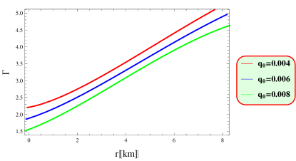
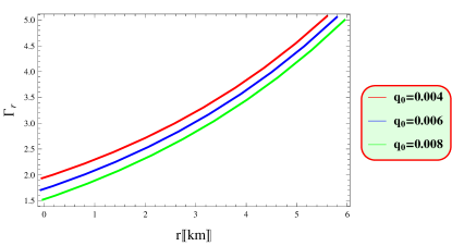
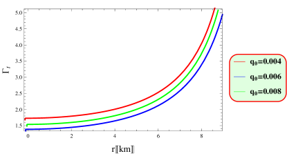
Figure 7: Graphical representations of adiabatic index relative to $r$.

Figure 7 demonstrates that our $f(Q)$ gravity model satisfies $\Gamma>\frac{4}{3}$, ensuring a stable anisotropic model for the PS with various values of $q_{0}$. The TOV equation is essential in theoretical astrophysics, particularly for understanding the equilibrium structure of spherical stellar objects. It describes the balance between gravitational forces and internal pressure, which is crucial for maintaining the stability of a star under its own gravity. The TOV equation is expressed as [42]

$$M_{G}(r)e^{\frac{\psi-\xi}{2}}\frac{1}{r^{2}}(\rho+p_{r})+\frac{dp_{r}}{dr}-\frac{2}{r}(p_{t}-p_{r})=0,$$ (41)

here the gravitational mass is defined as [43]

$$M_{G}(r)=4\pi\int(\mathbb{T}^{t}_{t}-\mathbb{T}^{r}_{r}-\mathbb{T}^{\phi}_{\phi}-\mathbb{T}^{\theta}_{\theta})r^{2}e^{\frac{\psi+\xi}{2}}dr.$$

Substituting these values and integrating this equation, we get

$$M_{G}(r)=\frac{1}{2}r^{2}e^{\frac{\xi-\psi}{2}}\psi^{\prime}.$$

Inserting this value into Eq.(41), we find that

$$\frac{1}{2}\psi^{\prime}(\rho+p_{r})+\frac{dp_{r}}{dr}-\frac{2}{r}(p_{t}-p_{r})=0.$$

We examine the hydrodynamic equilibrium of our model by applying the TOV equation within the framework of $f(Q)$ gravity

$$F_{a}+F_{g}+F_{h}+F_{Q}=0.$$

Analyzing the stability of a model under various forces is crucial. For an anisotropic charged compact object, stability is assessed by examining four key force components. The gravitational force $F_{g}$, the hydrostatic force $F_{h}$, the anisotropic force $F_{a}$ and the electromagnetic force $F_{Q}$. To ensure the model’s stable equilibrium, these forces must be properly balanced. In this study, we use the generalized TOV equation to analyze stability. These can be defined as

$$F_{a} = 2\frac{\chi}{r},\quad F_{g}=\frac{\psi^{\prime}(p_{r}+\rho)}{2},\quad F_{h}=-p_{r}^{\prime},$$

$$F_{Q} = p_{r}^{\prime}+\frac{\xi^{\prime}}{2}(\rho-p_{r})-\frac{2}{r}(p_{t}-p_{r}).$$

By substituting the values, we get

$$F_{a} = \frac{1}{r^{3}}\bigg{[}2e^{-\eta_{2}r^{2}}\bigg{(}\zeta\big{(}\eta_{0}^{2}r^{4}-\eta_{0}\eta_{2}r^{4}+5\eta_{0}r^{2}\big{)}-e^{\eta_{2}r^{2}}\bigg{(}\big{(}2\eta_{0}r^{4}+\eta_{0}r^{2}+2\eta_{2}r^{4}$$

$$+ \eta_{2}r^{2}\big{)}\zeta+2q_{0}^{2}r^{4}\bigg{)}+2\zeta r^{4}(\eta_{0}+\eta_{2})e^{2\eta_{2}r^{2}}\bigg{)}\bigg{]},$$

$$F_{g} = -\frac{1}{2r}\bigg{[}\eta_{0}\zeta e^{-\eta_{2}r^{2}}\bigg{(}\eta_{0}r^{2}\bigg{(}2r^{2}e^{2\eta_{2}r^{2}}-\big{(}2r^{2}+1\big{)}e^{\eta_{2}r^{2}}+3\bigg{)}+\eta_{2}r^{2}\bigg{(}e^{2\eta_{2}r^{2}}$$

$$\times 2r^{2}-\big{(}2r^{2}+1\big{)}e^{\eta_{2}r^{2}}-1\bigg{)}-2R^{2}\bigg{(}e^{\eta_{2}r^{2}}-1\bigg{)}\bigg{)}\bigg{]},$$

$$F_{h} = 2r\bigg{(}q_{0}^{2}-\big{(}\zeta e^{-\eta_{2}r^{2}}\big{(}\eta_{0}^{2}\big{(}-\eta_{2}r^{2}\big{)}+\eta_{0}\eta_{2}\big{(}\eta_{2}r^{2}-3\big{)}+\eta_{2}^{2}\big{)}\big{)}\bigg{)},$$

$$F_{Q} = \frac{1}{2r^{3}}\bigg{[}e^{-\eta_{2}r^{2}}\bigg{(}4\eta_{2}r^{2}\bigg{(}2e^{2\eta_{2}r^{2}}(\eta_{0}+\eta_{2})\zeta r^{4}+\big{(}(3\eta_{0}+\eta_{2})r^{2}\big{)}\zeta-e^{\eta_{2}r^{2}}$$

$$\times \bigg{(}q_{0}^{2}r^{4}+\big{(}(\eta_{0}+\eta_{2})\big{(}2r^{2}+1\big{)}r^{2}\big{)}\zeta\bigg{)}\bigg{)}+4\bigg{(}-4e^{2\eta_{2}r^{2}}\zeta(\eta_{0}+\eta_{2})r^{2}$$

$$\times \big{(}\eta_{2}r^{2}\big{)}-(3\eta_{0}+\eta_{2})\zeta+\bigg{(}\eta_{2}^{2}\big{(}2r^{2}+1\big{)}\zeta r^{2}+\big{(}2q_{0}^{2}r^{2}+\eta_{0}\big{(}4r^{2}+1\big{)}\zeta\big{)}$$

$$+ \big{(}q_{0}^{2}r^{4}+\big{(}2r^{2}+1\big{)}\big{(}\eta_{0}r^{2}+2\big{)}\zeta\big{)}\eta_{2}\bigg{)}e^{\eta_{2}r^{2}}\bigg{)}r^{2}-4\bigg{(}2e^{2\eta_{2}r^{2}}(\eta_{0}+\eta_{2})\zeta r^{4}$$

$$+ \big{(}\eta_{0}^{2}r^{4}-\eta_{0}\eta_{2}r^{4}+5\eta_{0}r^{2}\big{)}\zeta-e^{\eta_{2}r^{2}}\big{(}2q_{0}^{2}r^{4}+\big{(}2\eta_{0}r^{4}+2\eta_{2}r^{4}+\eta_{0}r^{2}$$

$$+ \eta_{2}r^{2}\big{)}\zeta\big{)}\bigg{)}(\eta_{0}+\eta_{2})\zeta r^{4}-\big{(}(3\eta_{0}+\eta_{2})r^{2}\big{)}\zeta+\big{(}\big{(}(\eta_{0}+\eta_{2})\big{(}2r^{2}+1\big{)}r^{2}$$

$$+ q_{0}^{2}r^{4}\big{)}\zeta\big{)}e^{\eta_{2}r^{2}}\bigg{)}-\bigg{[}r\bigg{(}\eta_{2}\bigg{(}2e^{2\eta_{2}r^{2}}r^{2}-e^{\eta_{2}r^{2}}\big{(}2r^{2}+1\big{)}-1\bigg{)}r^{2}+\eta_{0}\bigg{(}2$$

$$\times e^{2\eta_{2}r^{2}}r^{2}-e^{\eta_{2}r^{2}}\big{(}2r^{2}+1\big{)}+3\bigg{)}r^{2}-2\bigg{(}e^{\eta_{2}r^{2}}-1\bigg{)}\bigg{)}\zeta\bigg{(}2\bigg{(}2e^{2\eta_{2}r^{2}}\zeta r^{4}$$

$$\times r(\eta_{0}+\eta_{2})\big{(}\eta_{2}r^{2}\big{)}-\big{(}\eta_{2}^{2}r^{4}+3\eta_{0}\eta_{2}r^{4}+\eta_{2}r^{2}\big{)}\zeta-e^{\eta_{2}r^{2}}\bigg{(}q_{0}^{2}r^{4}+\big{(}2\eta_{0}r^{4}$$

$$+ 2\eta_{2}r^{4}\big{)}\zeta\bigg{)}\bigg{)}\bigg{(}e^{\eta_{2}r^{2}}\bigg{(}2q_{0}^{2}r^{2}+\eta_{2}\big{(}q_{0}^{2}r^{4}+\zeta\big{)}\bigg{)}+\eta_{2}\big{(}4\eta_{2}r^{2}\big{)}\zeta-\bigg{(}2r\bigg{(}e^{\eta_{2}r^{2}}$$

$$\times \big{(}q_{0}^{2}r^{4}+\zeta\big{)}\bigg{)}+\big{(}2\eta_{2}^{2}r^{4}-\eta_{2}r^{2}\big{)}\zeta\bigg{)}\bigg{(}2e^{2\eta_{2}r^{2}}\big{(}2\eta_{2}^{2}r^{4}+5\eta_{2}r^{2}+2\big{)}\zeta r^{2}(\eta_{0}$$

$$+ \eta_{2})-\eta_{2}\big{(}6\eta_{0}r^{2}+2\eta_{2}r^{2}\big{)}\zeta-e^{\eta_{2}r^{2}}\bigg{(}2\eta_{2}^{2}\zeta r^{4}+2\big{(}q_{0}^{2}+2\eta_{0}\zeta\big{)}r^{2}+\eta_{2}$$

$$\times \big{(}q_{0}^{2}r^{4}+\big{(}\eta_{0}r^{4}+\big{(}4r^{2}-1\big{)}\big{)}\zeta\big{)}\bigg{)}\bigg{)}\bigg{)}\bigg{)}\bigg{]}\bigg{[}\bigg{(}\zeta\big{(}\eta_{2}^{2}r^{4}+3\eta_{0}\eta_{2}r^{4}+\eta_{2}r^{2}\big{)}$$

$$+ 2e^{2\eta_{2}r^{2}}(\eta_{0}+\eta_{2})\big{(}\eta_{2}r^{2}\big{)}\zeta r^{4}+e^{\eta_{2}r^{2}}\bigg{(}q_{0}^{2}r^{4}+\big{(}2\eta_{0}r^{4}+2\eta_{2}r^{4}\big{)}\zeta\bigg{)}\bigg{)}^{2}\bigg{]}^{-1}\bigg{)}\bigg{]}.$$

We have illustrated the condition for stable equilibrium using a graphical representation. Figure 8 shows that equilibrium is attained when the combined forces of $F_{a}$, $F_{g}$, $F_{h}$ and $F_{Q}$ sum to zero. This confirms that the PS model remains stable across different values of $q_{0}$. The figure presents two distinct graphs that show the behavior of $F_{Q}$. In one where $F_{Q}=0$, it indicates no electromagnetic force and the stability of the system depends solely on the balance of the gravitational, hydrostatic and anisotropic forces. If these forces are in balance, the system can remain stable, though the absence of electromagnetic force might lead to variations in pressure and structure. The other graph shows $F_{Q}\neq 0$, where the electromagnetic force provides additional repulsion, helps to counteract gravitational collapse and plays a key role in maintaining stability.

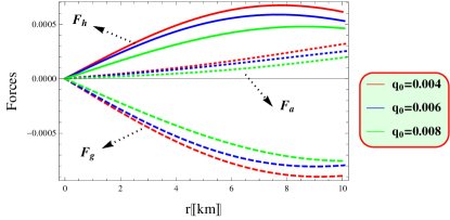
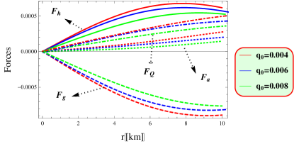
Figure 8: Graphs of TOV equation as functions $r$.

5 Equation of State Parameter and Compactness

Here, we apply the subsequent equations [24]

$$p_{r}(\rho)\approx v^{2}_{r}(\rho-\rho_{I}),\quad p_{t}(\rho)\approx v^{2}_{t}(\rho-\rho_{II}).$$

In this model, $\rho_{I}$ and $\rho_{II}$ represent the densities at the surface of the star, related to the radial and tangential pressures, respectively. While $\rho_{I}$ can make $p_{r}$ zero, $\rho_{II}$ does not have the same effect on the $p_{t}$. The model helps us figure out both the speed of sound and the surface density of the star. For instance, with $q_{0}=0.004$, inserting Eqs.(39) and (40), gives us $v_{r}^{2}\approx 0.793,~{}v_{t}^{2}\approx 0.851$, $\rho_{I}\approx 5.01\times 10^{14}$ g/cm³ and $\rho_{II}\approx 3.99\times 10^{14}$ g/cm³. Similarly, for $q_{0}=0.006$, the values are $v_{r}^{2}\approx 0.789,~{}v_{t}^{2}\approx 0.842$, $\rho_{I}\approx 5.04\times 10^{14}$ g/cm³ and $\rho_{II}\approx 4.2\times 10^{14}$ g/cm³. Also, for $q_{0}=0.008$, we find $v_{r}^{2}\approx 0.785,~{}v_{t}^{2}\approx 0.717$, $\rho_{I}\approx 0.833\times 10^{14}$ g/cm³ and $\rho_{II}\approx 4.4\times 10^{14}$ g/cm³.

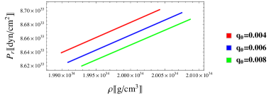
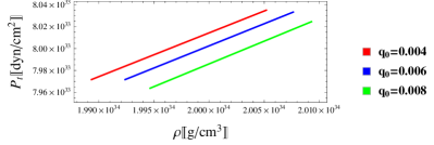
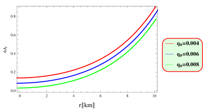
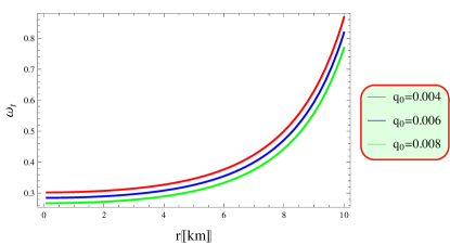
Figure 9: Graphs of EoS versus $r$.

The EoS parameter, denoted as $\omega$, is expressed as $\omega=\frac{p}{\rho}$. In astrophysics and cosmology, this parameter is crucial for understanding the behavior of different components of the universe. A valid model requires that both the radial EoS parameter $(\omega_{r}=\frac{p_{r}}{\rho})$ and the tangential EoS parameter $(\omega_{t}=\frac{p_{t}}{\rho})$ to be within the range of $[0,1]$ [44]. By substituting Eqs.(33)-(34) into the above formulas, we obtain

$$\omega_{r} = \bigg{[}-e^{\eta_{2}r^{2}}\bigg{(}\zeta\big{(}2\eta_{0}r^{4}+\eta_{0}r^{2}+2\eta_{2}r^{4}+\eta_{2}r^{2}\big{)}+q_{0}^{2}r^{4}\bigg{)}+2\zeta r^{4}e^{2\eta_{2}r^{2}}$$

$$\times (\eta_{0}+\eta_{2})+\zeta\big{(}3\eta_{0}r^{2}+\eta_{2}r^{2}\big{)}\bigg{]}\bigg{[}e^{\eta_{2}r^{2}}\bigg{(}q_{0}^{2}r^{4}-\zeta\bigg{)}-\zeta\big{(}2\eta_{2}r^{2}\big{)}\bigg{]}^{-1},$$

$$\omega_{t} = \bigg{[}r^{2}\bigg{(}\bigg{(}\zeta e^{-\eta_{2}r^{2}}\bigg{(}\eta_{0}r^{2}(\eta_{0}-\eta_{2})+(2\eta_{0}-\eta_{2})\bigg{)}\bigg{)}-q_{0}^{2}r^{2}\bigg{)}\bigg{]}$$

$$\times \bigg{[}\zeta e^{-\eta_{2}r^{2}}\bigg{(}2\eta_{2}r^{2}-1\bigg{)}+\zeta-q_{0}^{2}r^{4}\bigg{]}^{-1}.$$

Figure 9 displays the best-fit EoS for the PS. It shows how density and radial pressure change with different values of $q_{0}$, align well with a linear EoS pattern. Similarly, the tangential EoS exhibits a strong relationship with a linear model. These EoSs are primarily accurate near the star’s center and throughout its interior, within the the specified range $[0,1]$ [45].

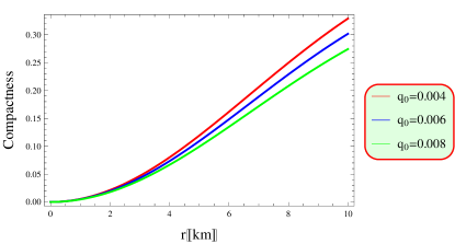
Figure 10: Graph of compactness versus $r$.

The compactness function $\varpi=2M(r)/r$ is essential for evaluating the star’s stability. For a star to be stable, its compactness must be less than $4/9$ [46]. This criterion helps to make sure that the star’s gravity is not strong enough to cause it to collapse. Therefore, it is important to check that $\varpi$ remains below this limit to ensure the star’s stability.

$$\varpi=4\pi\zeta\bigg{(}1-e^{-\eta_{2}r^{2}}\bigg{)}-\frac{4}{5}\pi q_{0}^{2}r^{4}.$$

Figure 10 demonstrates that the compactness increases gradually while remaining within the specified limit.

6 Summary and Discussion

In this paper, we have examined how the $f(Q)=\zeta Q$ gravity model affects the structure and stability of charged PS. By considering an anisotropic fluid and using the KB ansatz for the star’s interior, we have determined key constraints on the model parameters, especially the value of $\zeta$. We have investigated the charge intensity $q_{0}$ which influenced our model through both numerical calculations and graphical representations. The key features are outlined as follows.

• We have found that the density and both radial/tangential pressures are highest at the core of the star and decrease towards the surface. Importantly, the radial pressure drops to zero at the surface of the star. As the charge intensity increases, the energy density and pressure go down. However, the steadily decreasing pattern of these profiles remains consistent in this model (Figure 1).

• The anisotropy consistently rises towards the star’s surface while still fulfilling stability requirements (Figure 2). This behavior aligns with theoretical predictions and confirms the physical viability of the proposed stellar model.

• The mass of the PS increases consistently and uniformly as its radius expands (Figure 3). This behavior aligns with the stability of the PS.

• We have observed that the redshift function keeps increasing for different values of $q_{0}$ (Figure 4). It always stays below the maximum value of 5.211 which is the highest value obtained from observational data.

• We have examined the energy conditions for various values of $q_{0}$ and demonstrated that the PS model satisfies all the energy requirements (Figure 5). This confirms that our model is physically viable.

• It is found for various values of $q_{0}$ the expressions $(0\leq v_{r}^{2}\leq 1)$ and $(0\leq v_{t}^{2}\leq 1)$ are satisfied ((Figure 6)) that confirm the stability and causality requirements. Furthermore, our analysis reveals that the condition $(0\leq v_{t}^{2}-v_{r}^{2}\leq 1)$ is satisfied throughout the pulsar’s interior which indicates a stable anisotropic stellar structure.

• We have observed that the adiabatic index $\Gamma$ is greater than $\frac{4}{3}$, indicating that the PS remains physically stable for different values of $q_{0}$ (Figure 7).

• The equilibrium is achieved when the total of the forces $F_{a}$, $F_{g}$, $F_{h}$ and $F_{Q}$ equals to zero (Figure 8). This ensures a stable model for the PS for various values of $q_{0}$.

• The EoS for the PS shows a strong linear relationship between density and radial pressure across all values of $q_{0}$. The tangential pressure also fits well with a linear model. These relationships hold true near the center of the star and throughout its interior, especially within the range of 0 to 1 (Figure 9).

• The compactness gradually rises inside the star and remains within the limit of $\varpi<4/9$ for various values of $q_{0}$ (Figure 10).

It is noteworthy that $f(Q)$ gravity enables the construction of realistic models adhering to essential principles for static spherically symmetric spacetime. We have successfully developed a stable and physically viable model of a charged PS using $f(Q)$ gravity. Our findings show that this theory meets theoretical stability criteria and aligns well with observational data. The inclusion of charge significantly influences the star’s structure, affecting its mass, radius and stability. Despite these variations, the charged model remains stable and physically viable. Our results are consistent with recent work in $f(Q)$ gravity [28], reinforcing the validity of pulsar studies within this framework and suggesting future research could provide new insights into gravity and compact objects.

Data Availability: No data was used for the research described in this paper.

References

- [1] Riess, A.G. et al.: Astron. J. 116(1998)1009; Perlmutter, S. et al.: Astrophys. J. 517(1999)565.
- [2] Sahni, V. and Starobinski, A.: Int. J. Mod. Phys. D 9(2000)373.
- [3] Yang, R.J. and Zhang, S.N.: Mon. Not. Roy. Astron. Soc. 407(2010)1835.
- [4] Velten, H.E.S. et al.: Eur. Phys. J. C 74(2014)3160.
- [5] Wang, D. et al.: Eur. Phys. J. C 79(2019)211; Mandal, S. et al.: Phys. Dark Universe 28(2020)100551; Yerramsetti, Y. et al.: Eur. Phys. J. C 79(2020)1020; Wang, D.: Phys. Dark Universe 28(2020)100545; Arora, S. et al.: Classical Quantum Grav. 37(2020)205022.
- [6] Weyl, H.: Sitzungsber. Preuss. Akad. Wiss. 465(1918)01; Dirac, P.A.M.: Proc. R. Soc. London A 333(1973)403; Hehl, F.W. et al.: Rev. Mod. Phys. 48(1976)393; Hehl, F.W. et al.: Phys. Rep. 258(1995)1.
- [7] Aldrovandi, R. and Pereira, J.G.: Teleparallel Gravity: An Introduction (Springer, 2013).
- [8] Maluf, J.W.: Ann. Phys. 525(2013)339.
- [9] Haghani, Z. et al.: J. Cosmology Astropart. Phys. 10(2012)061.
- [10] Nester, J.M. and Yo, H.J.: Chin. J. Phys. 37(1999)113.
- [11] Jimenez, J.B., Heisenberg, L. and Koivisto, T.: Phys. Rev. D 98(2018)044048.
- [12] Conroy, A. and Koivisto, T.: Eur. Phys. J. C 78(2018)923; , L. et al.: Phys. Rev. D 97(2018)124025; Delhom-Latorre, A., Olmo, G.J. and Ronco, M.: Phys. Lett. B 780(2018)294; Harko, T. et al.: Phys. Rev. D 98(2018)084043; Hohmann, M. et al.: Phys. Rev. D 99(2019)024009.
- [13] Lazkoz, R. et al.: Phys. Rev. D 100(2019)104027.
- [14] Shekh, S.H.: Phys. Dark Universe 33(2021)100850.
- [15] Frusciante, N.: Phys. Rev. D 103(2021)044021.
- [16] Sharif, M. and Ajmal, M.: Chin. J. Phys. 88(2024)706; Phys. Scr. 99(2024)085039.
- [17] Sharif, M. and Ajmal, M.: Phys. Dark Universe 46(2024)101572.
- [18] Zand, J.I.T. et al.: Astron. Astrophys. 345(1999)100.
- [19] van Kerkwijk, M.H. et al.: Astrophys. J. 563(2001)41; Markwardt, C.B. and Swank, J.H.: The Astronomer Telegram 495(2005)1; Patruno, A. et al.: The Astronomer Telegram 2407(2010)1.
- [20] Bozzo, E., Kuulkers, E. and Ferrigno, C.: The Astronomer Telegram 7106(2015)1.
- [21] Altamirano, D. et al.: Astrophys. J. 674(2008)L45.
- [22] Kramer, M. et al.: Science 314(2006)97.
- [23] Nashed, G.G.L.: Astrophys. J. 950(2023)129.
- [24] Nashed, G.G.L.: Eur. Phys. J. C 83(2023)698; Nashed, G.G. and Capozziello, S.: Eur. Phys. J. C. 84(2024)17.
- [25] Maurya, S.K., and Gupta, Y.K.: Astrophys. Space Sci. 353(2014)657.
- [26] Sharif, M. and Waseem, A.: Int. J. Mod. Phys. D 28(2019)1950033.
- [27] Sharif, M. and Gul, M.Z.: Fortschr. Phys. 71(2023)2200184.
- [28] Bhattacharjee, D. and Chattopadhyay, P.K.: arXiv preprint [arXiv:2407.10587[gr-qc]].
- [29] Sharif, M. and Ibrar, I.: Chin. J. Phys. 89(2024)1578.
- [30] Goncalves, V.P. and Lazzari, L.: Phys. Rev. D 102(2020)034031.
- [31] Sharif, M., Gul, M.Z. and Fatima, N.: New Astron. 109(2024)102211.
- [32] Krori, K.D. and Barua, J.: J. Phys. A 8(1975)508.
- [33] zel, F., Gver, T. and Psaltis, D.: Astrophys. J. 693(2009)1775.
- [34] Deb, D. et al.: Ann. Phys. 387(2017)239.
- [35] Ivanov, B.V.: Phys. Rev. D 65(2002)104011.
- [36] Barraco, D.E., Hamity, V.H. and Gleiser, R.J.: Phys. Rev. D 67(2003)064003; Bhmer, C. and Harko, T.: Class. Quantum Grav. 23(2006)6479.
- [37] Zeldovich, Y.B. and Novikov, I.D.: Relativistic Astrophysics. Vol. 1: Stars and Relativity (Univ. Chicago Press, 1971).
- [38] Abreu, H. et al.: Class. Quantum Grav. 24(2007)4631.
- [39] Herrera, L.: Phys. Lett. A 165(1992)206.
- [40] Chandrasekhar, S.: Astrophys. J. 140(1964)417; Chan, R., Herrera, L. and Santos, N.: Mon. Not. R. Astron. Soc. 265(1993)533.
- [41] Heintzmann, H. and Hillebrandt, W.: Astron. Astrophys. 38(1975)51.
- [42] Tolman, R.C.: Phys. Rev. 35(1930)896.
- [43] Tolman, R.C.: Phys. Rev. 55(1939)364; Oppenheimer, J.R. and Volkoff, G.M.: Phys. Rev. 55(1939)374.
- [44] Shamir, M.F. and Zia, S.: Eur. Phys. J. C 77(2017)448.
- [45] Singh, K.N. et al.: Eur. Phys. J. A 53(2017)21.
- [46] Buchdahl, A.H.: Phys. Rev. D 116(1959)1027.