Simulations for estimation of random effects and overall effect in three-level meta-analysis of standardized mean differences using constant and inverse-variance weights
Abstract
We consider a three-level meta-analysis of standardized mean differences. The standard method of estimation uses inverse-variance weights and REML/PL estimation of variance components for the random effects.
We introduce new moment-based point and interval estimators for the two variance components and related estimators of the overall mean. Similar to traditional analysis of variance, our method is based on two conditional statistics with effective-sample-size weights. We study, by simulation, bias and coverage of these new estimators. For comparison, we also study bias and coverage of the REML/PL-based approach as implemented in rma.mv in metafor. Our results demonstrate that the new methods are often considerably better and do not have convergence problems, which plague the standard analysis.
Keywords hierarchical model, inverse-variance weights, effective-sample-size weights, random effects, heterogeneity
1 Introduction
When viewed as a multilevel model (Raudenbush and Bryk [1985], Goldstein et al. [2000]), the standard random-effects model of meta-analysis is a two-level hierarchical model. Typically, the level-1 units comprise the sample within each study, and the level-2 units are the studies. A three-level model involves a further level of structure; for example, the studies may be nested within clusters. Konstantopoulos [2011] discusses the traditional analysis of a three-level model in detail. Cheung [2014] formulated a three-level model in the framework of structural-equation modelling. Multilevel meta-analysis is implemented in the rma.mv procedure in metafor [Viechtbauer, 2010]. Traditional analysis uses REML-based estimation of the variance components for the random effects and profile-likelihood estimation of their confidence intervals.
In a meta-analysis involving three levels, one can apply moment estimation similar to that in analysis of variance, subdividing the total variation into within and between components. Our approach uses constant weights based on effective sample sizes (SSW).
In a related development, in multivariate meta-analysis, Jackson et al. [2024] proposed a method of moment-based estimation of the between-study covariance matrix (analogous to the heterogeneity variance in the usual random-effects model). In that method, the weights for estimating the overall effects involve an estimate of the covariance matrix, which is then updated to reflect the current estimate of the overall effects. By using fixed weights, we avoid that complication.
In a systematic review of multilevel meta-analyses, Fernández-Castilla et al. [2020] listed existing simulation studies (their Table 1) and the parameters from 178 actual meta-analyses in behavioral, social, biological, and medical sciences (their Tables 3–5). Our simulation scenarios were largely guided by these tables. Of those 178 meta-analyses, 162 fitted the three-level model.
For the case of standardized mean difference (SMD) as the effect measure, our simulation study evaluated our novel moment-based method of estimation in a three-level meta-analysis and compared it with the standard REML/PL-based methods implemented in rma.mv in metafor.
2 A three-level hierarchical model for meta-analysis
We consider a 3-level hierarchical model involving clusters of studies: studies in cluster () and sample size for study in cluster (). The model includes random variation at each level: level-1, within-study random errors ; level-2, within-cluster between-studies random effects ; and level-3, between-clusters random effects ; where and are unit matrices of dimension and , respectively. In this model, the level-2 parameter, , is not cluster-specific, so estimation can use the full data. Cluster-specific variances, , would require within-cluster estimation. Our methods can handle the latter scenario, but we have not done any simulations for it.
Similar to a two-level meta-regression model with random effects, for cluster we observe a -vector of summary statistics,
| (2.1) |
where is an effect of cluster , is a vector of 1’s of dimension , is a design matrix, is a -vector of fixed effects (without an intercept), and and represent independent between- and within-study variation, respectively. It follows that, conditionally, .
To write the model in Equation (2.1) in terms of the stacked vector of length , we define the parameter vector of dimension , and the design matrices , where is the Kronecker delta ( if and 0 otherwise). We form the design matrix by stacking the . Thus, also using stacked error vectors and , Equation (2.1) becomes
| (2.2) |
This model differs from the standard meta-regression model only by including in the -vector of random intercepts ; the studies in cluster have the same .
We model the intercepts via a mixed-effects meta-regression and a level-3 random effect:
| (2.3) |
where is a matrix of fixed effects, is a -vector of unknown coefficients, is a random-effects design matrix, is an -vector of random effects, and . The variance is . Thus, the unconditional covariance matrix for cluster is
| (2.4) |
where is the matrix of 1’s. The full covariance matrix of the stacked vector , denoted by , is the block-diagonal matrix of the matrices .
3 Estimation
As in ANOVA.we approach estimation by subdividing the total variation into within and between components and using moments. Thus, we work with Equations (2.1) and (2.3) separately.
3.1 Estimating 2nd-level parameters (within-cluster analysis)
At level 2, conditionally on the values of , we can estimate and as in a standard meta-regression.
To accommodate various choices of weights, we introduce , a symmetric matrix of full rank. Then from Equation (2.2) and
| (3.1) |
is an unbiased estimator of with conditional covariance
| (3.2) |
where . The maximum-likelihood-based estimator corresponds to (i.e., to inverse-variance weights). For ML/IV, given by Equation (3.1) needs to be calculated simultaneously with . For any fixed , however, and can be estimated separately.
The residuals based on are , where is a hat matrix, similar to that in least-squares regression. As projections, and are idempotent. That is, . Also, .
Moment estimation of the variance component is based on the generalized statistic, a quadratic form in the residuals:
| (3.3) |
(discussed by DerSimonian and Kacker [2007]). Given unbiased estimators and a nonrandom matrix, and denoting the weight matrix by , and , where the weight is applied to in Equation (3.3). Hence, a moment estimator of is
| (3.4) |
The distribution of is that of a quadratic form in normal random variables, and we can obtain a confidence interval for from percentage points of an approximation to this distribution under the hypothesis of no heterogeneity.
In the simplest case (i.e., no meta-regression), and the within-cluster model in Equation (2.1) is the standard random-effects model of meta-analysis. Then the only unknown parameters are . For a block-diagonal matrix , in which is , Equation (3.1) results in , where and . The conditional variances are for .
3.2 Estimating 3rd-level parameters (between-cluster analysis)
At level 3 the models for (Equation (2.3)) share the fixed effects (), the covariance matrix , and the variance . Since , the unconditional expected value . In matrix form, for the matrix with rows . Hence, for a symmetric matrix of a full rank,
| (3.5) |
is an unbiased estimator of with covariance
| (3.6) |
Next, . Since the are independent, , and .
Now the “residuals” , where is an idempotent matrix.
Similar to the 2nd-level case, we consider a generalized statistic
| (3.7) |
Given unbiased estimators and a nonrandom matrix, and denoting the weight matrix by , We have already estimated and , but equating to provides only one equation with parameters. Only when is known or zero can we find a moment estimator of à la DerSimonian and Kacker [2007]:
| (3.8) |
The distribution of is that of a quadratic form in normal random variables, and a confidence interval for can be obtained from percentage points of an approximation to this distribution under the hypothesis of no heterogeneity.
4 Simulation design and results
Our main objective was to evaluate our moment-based method of estimation in a 3-level meta-analysis and to compare it with standard methods of hierarchical meta-analysis (rma.mv in metafor) for standardized mean difference as an effect measure.
4.1 Simulation design
At the end of Section 3.1 we introduced, for generality, block-diagonal matrices . In our simulations we considered comparative studies with two arms, C and T. We used diagonal matrices ), where are within-study effective sample sizes, is the total sample size of a study with and observations in the control and treatment arms. Then are the sample-size-weighted means of the elements of , with . The matrix in Equation (3.5) was also a diagonal matrix: .
In our simulations we took in Equation (2.1), and and in Equation (2.3). Thus, the 3-level model of meta-analysis had one fixed effect (the overall mean, ) and two variance components ( at level 2, and at level 3).
To emphasize that we are dealing with meta-analysis of SMD, we change the notation for the effects in what follows. We denote the overall true effect ( previously) by and the cluster-specific means by .
Our simulations varied five parameters: the overall true effect , the between-studies and between-clusters variances (), the number of clusters (), the (equal) number of studies in each cluster (), and the studies’ (equal) total sample size (). The proportion of observations in the control arm was fixed at . Table 1 lists the values of each parameter.
Given a true effect , we generated the cluster effects from a normal distribution with mean and variance . Next, the means for within-cluster studies were generated by adding -distributed within-study shifts. Observed SMD values were then generated from scaled noncentral -distributions with noncentrality parameters based on the study means. Finally, Hedges’s correction [Hedges, 1983] was used to obtain values of Hedges’s .
Overall, we considered 1600 combinations of parameters. R statistical software [R Core Team, 2016] was used for the simulations.
In addition to the effective-sample-size-based methods for the 3-level model introduced in Section 3, we included, for comparison, REML and profile-likelihood-based methods [Hardy and Thompson, 1996] (implemented in the rma.mv procedure in metafor [Viechtbauer, 2010]).
For assessing heterogeneity in a 3-level model, we used the matrices ( and ). We used approximations to their distributions (as quadratic forms in approximately normal variables) to obtain empirical level and power for heterogeneity tests based on and , and confidence intervals for and . For these distributions, we used the R package CompQuadForm [Duchesne and de Micheaux, 2010]. The Farebrother approximation [Farebrother, 1984] did not work well for the 3-level case because of sparseness of the resulting covariance matrix, so we used the Davies algorithm [Davies, 1980] instead.
User-friendly R programs implementing our methods are available at osf.io/zgtpn .
Initially, we aimed at a total of repetitions for each combination of parameters. However, rma.mv, which we used with its default optimizer nlminb, was rather slow for . Therefore, our final series of simulations aimed for repetitions for all combinations of parameters. Even then, rma.mv using nlminb struggled to converge for when . For these values, time constraints prevented us from obtaining simulation results beyond . Appendix A reports results on non-convergence rates of rma.mv.
We compared the performance of the two classes of methods on
-
•
Bias in estimation of the overall effect ;
-
•
Coverage of the overall effect by 95% confidence intervals, centered on the respective estimate of and based on quantiles from the normal distribution and the -distribution with df;
-
•
Bias in estimation of the variance components and ;
-
•
Coverage of the 95% confidence intervals for and .
We also studied empirical levels of the heterogeneity tests based on the and statistics using the Davies approximation [Davies, 1980] to the distribution of quadratic forms in normal variables.
| Parameter | Values |
|---|---|
| (number of clusters) | 5, 10, 25, 50 |
| (number of studies in a cluster) | 2, 5, 10, 20 |
| (study size, total of the two arms) | 20, 40, 100, 200, 1000 |
| (fraction of observations in the control arm) | 1/2 |
| (true value of SMD) | , , , |
| (variances of random effects at levels 2 and 3) | 0, 0.02, 0.1, 0.2, 0.5 |
4.2 Summary of simulation results
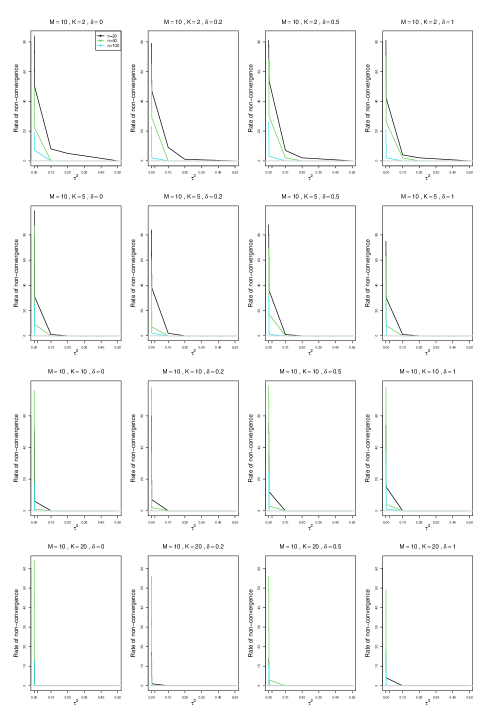
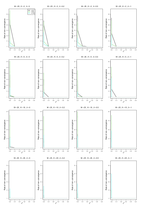
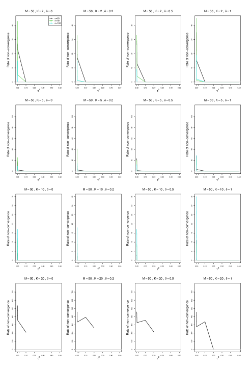
4.2.1 Non-convergence rates in three-level analysis as implemented in metafor (Appendix A)
Our simulations used the default nlminb optimizer for rma.mv. Here we report on the non-convergence rates, defined as output of zero length. Additionally, even when there was some output, the search for confidence limits for either or both of the variance components may not have converged. Typically, the non-convergence rates of those confidence limits were somewhat higher, up to 9.5 percentage points higher for and up to 8.3 percentage points higher for , but we do not report on them.
The non-convergence rates were considerable (7 to 11%) when the variance components were close to zero, but they decreased and then became negligible further on. They did not depend on the overall effect , but they improved greatly with increases in the number of studies , in the study size , and, to some extent, in the number of clusters for .
They increased dramatically for and , reaching up to 45% at when .
The new moment-based methods encountered no instances of non-convergence.
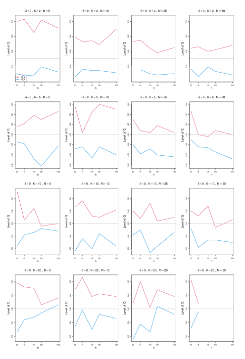
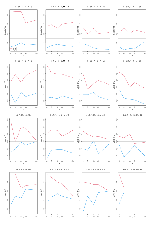
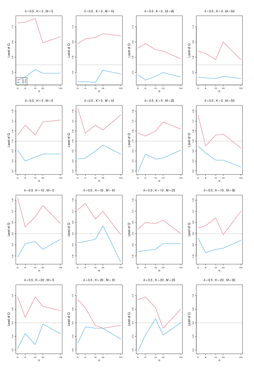
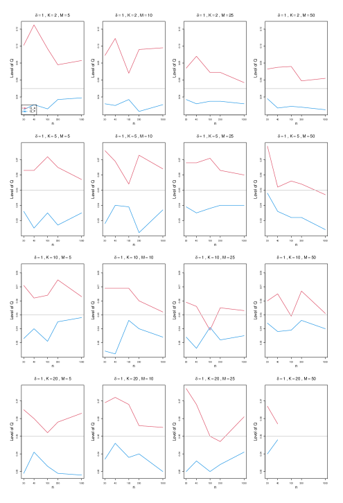
4.2.2 Empirical level of the two tests at for heterogeneity (Appendix B)
Empirical levels of were typically above the nominal level (range .039 to .125), and those of were below the nominal level (range .019 to .058).
The results do not improve uniformly with but appear rather heterogeneous. This behavior may be due to the relatively small number of repetitions. Typically, empirical levels were closer to nominal for larger values of , , and . The levels seem not to depend on .
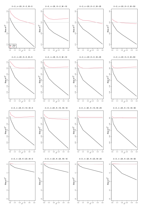
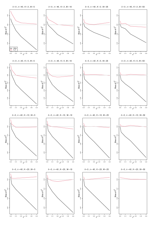
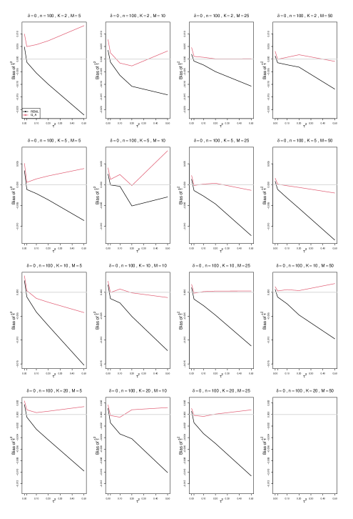
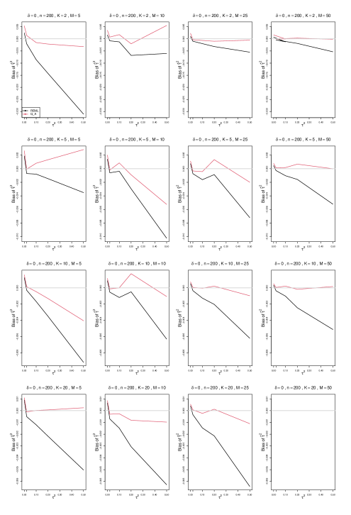
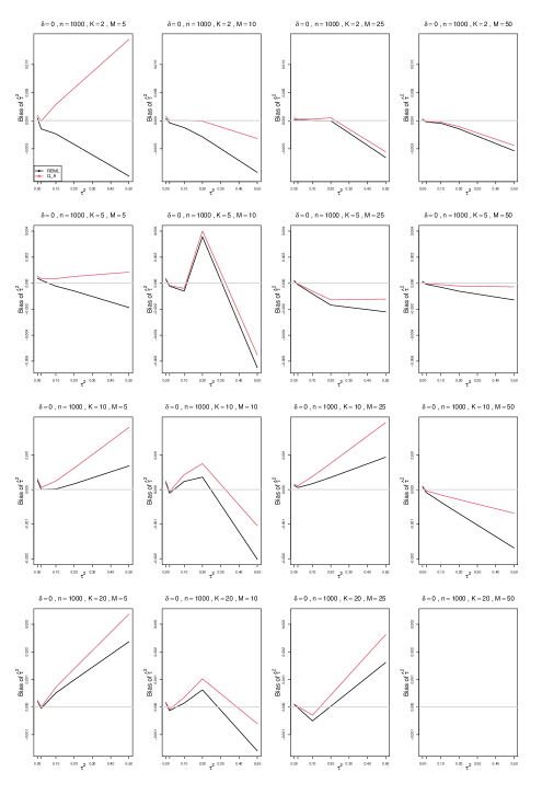
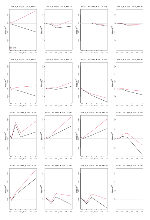
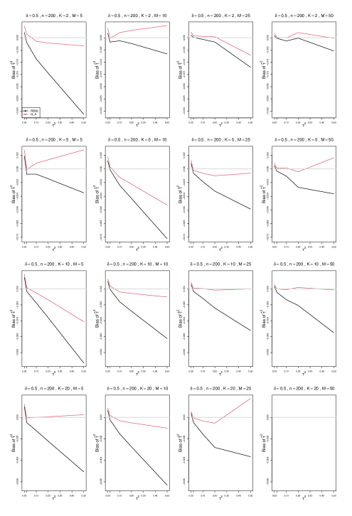
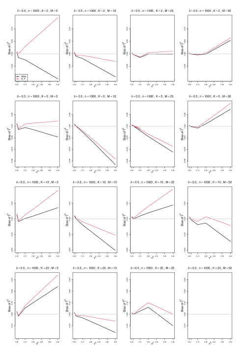
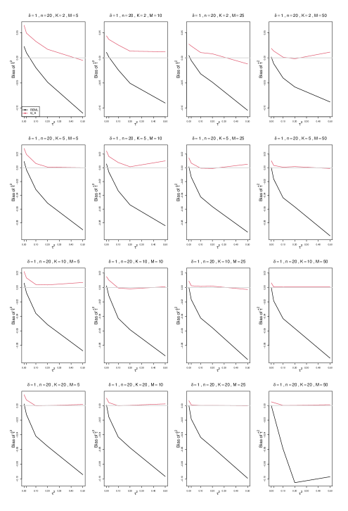
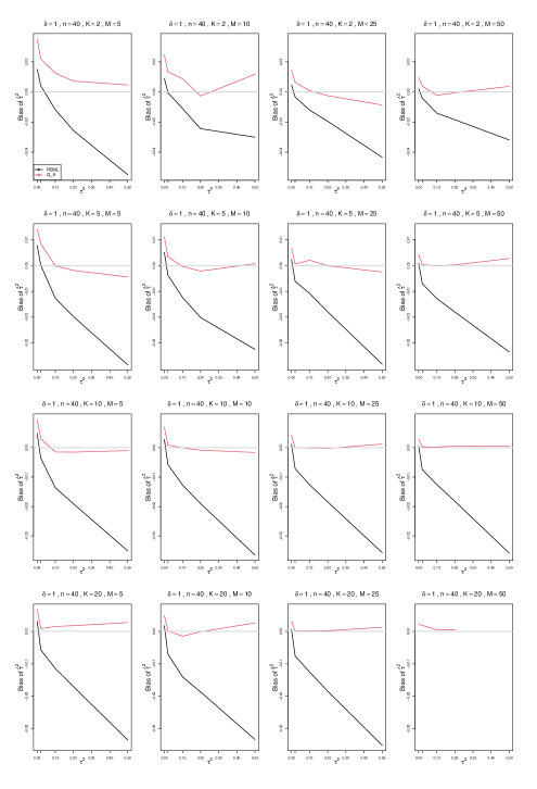
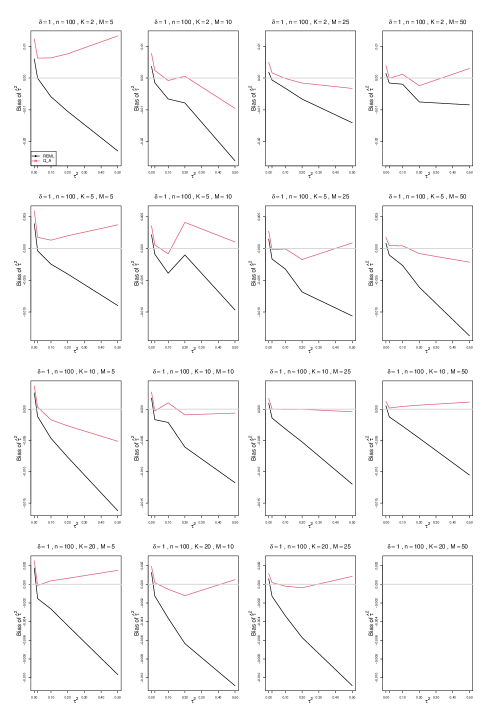
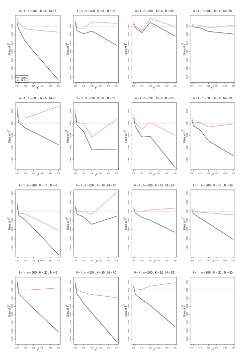
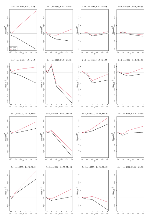
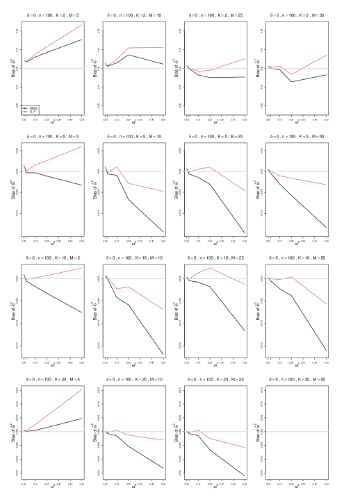
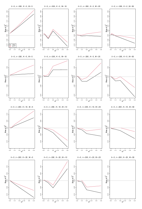
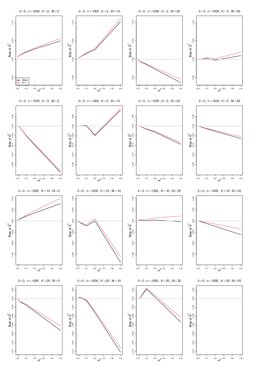
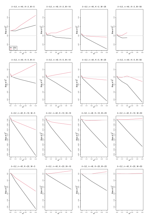
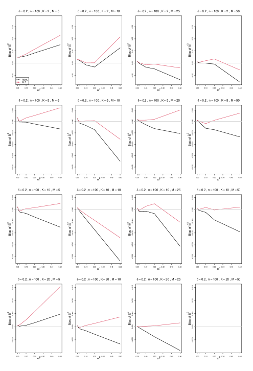
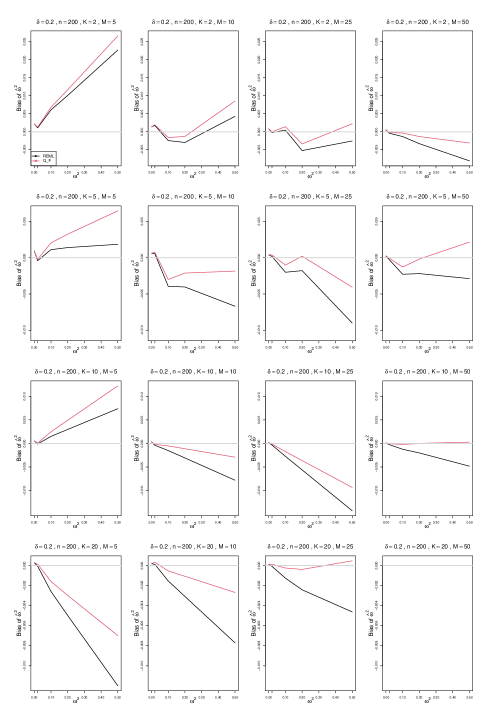
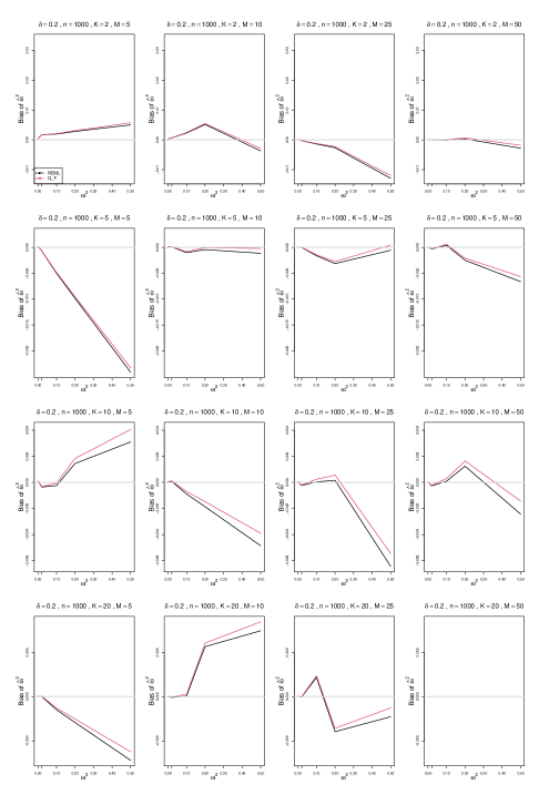
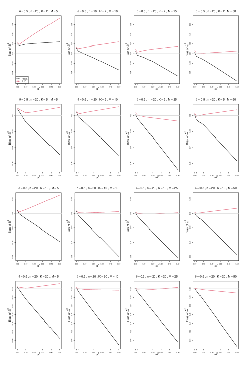
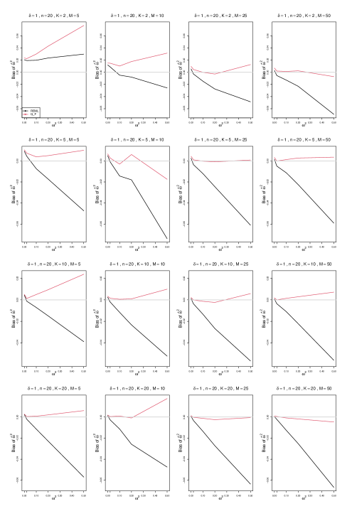
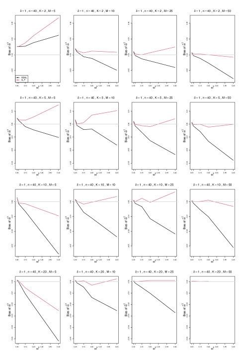
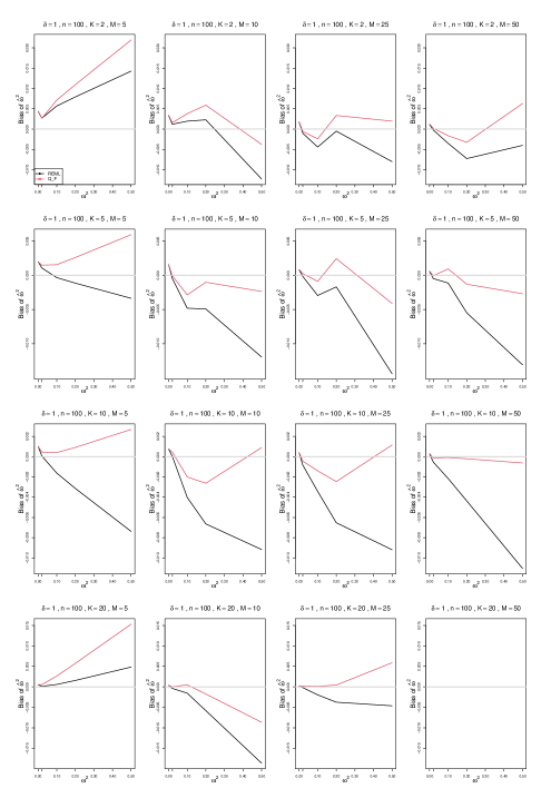
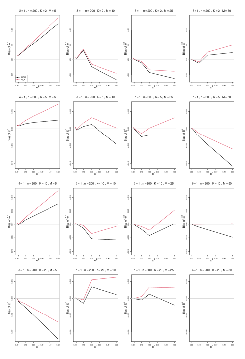
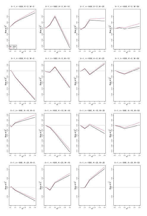
4.2.3 Bias of point estimators of (Appendix C)
The REML and -based estimators of were both positively biased at , the -based estimator somewhat more. However, the REML estimator had increasingly negative bias for , whereas the -based estimator was almost unbiased throughout.
The bias of REML was greatest for and , reaching at when and . Though still increasingly negative, it was negligible for when . When , it was still considerable for large . As an example, when , and , the bias of the REML estimator was about at .
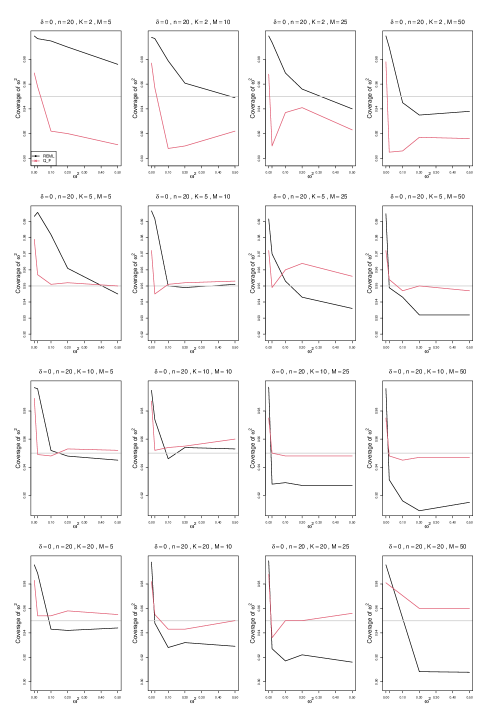
4.2.4 Coverage of interval estimators of (Appendix D)
Coverage of interval estimators of did not depend much on .
When , , and , coverage of the -based intervals was about , and the coverage of the -based intervals was higher for and somewhat lower for .
The coverage of the -based intervals was close to nominal for larger and when , whereas the PL-based coverage deteriorated to unacceptably low levels. It was only 20% for and .
For , the coverage of PL improved and typically was above 93%. Coverage of was close to nominal. For , PL coverage was close to nominal, and the -based intervals often had higher coverage, at 96 to 97%.
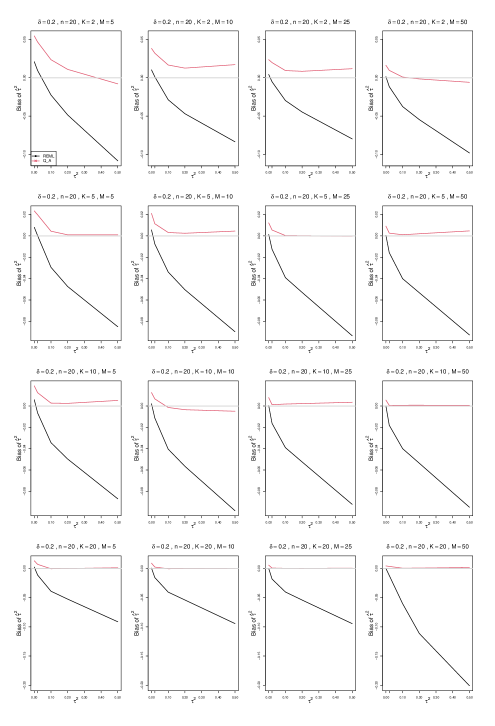
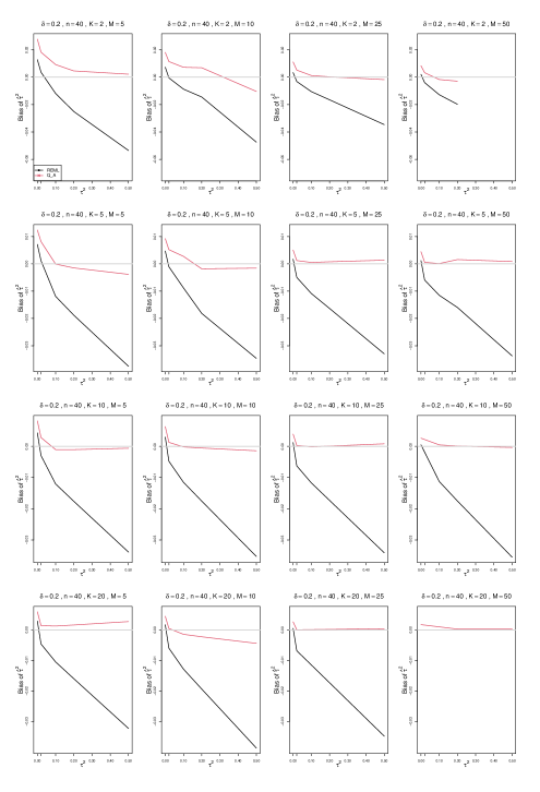
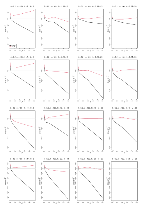
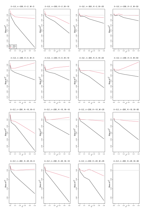
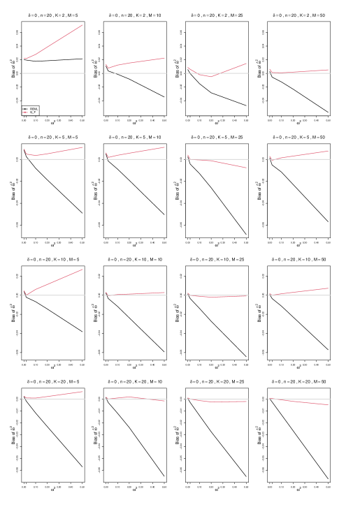
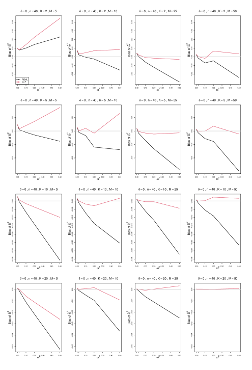
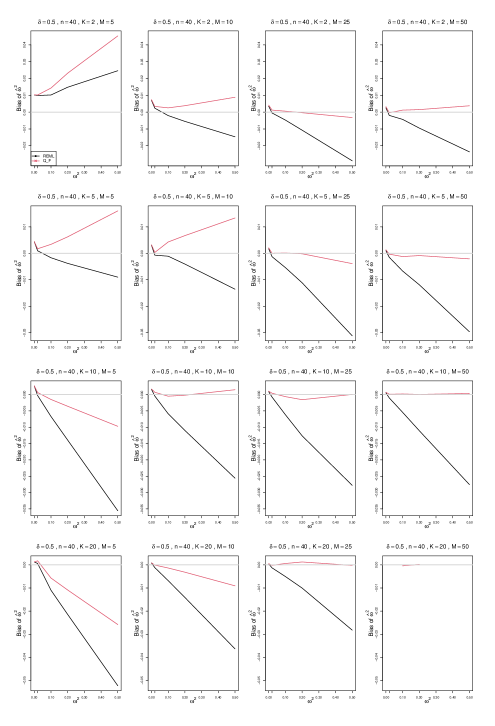
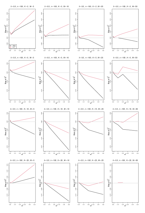
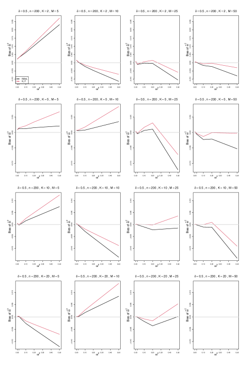
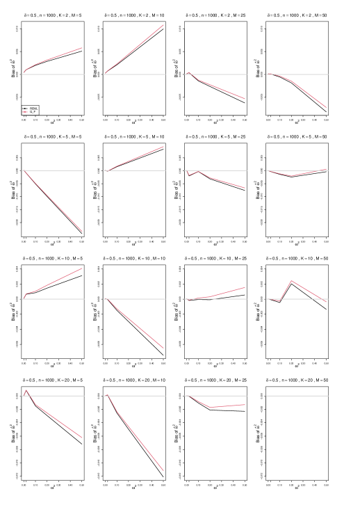
4.2.5 Bias of point estimators of (Appendix E)
Both estimators of were somewhat positively biased at zero, the -based estimator somewhat more. For larger , the REML estimator was typically negatively biased, whereas the -based estimator was somewhat positively biased; both biases increased with . When , , and , the maximum bias was 0.02 for REML and up to 0.065 for . For larger and , was almost unbiased, and the bias of REML was at worst .
For , the pattern was similar, though the bias of REML decreased with . For , the bias of REML was very small, at worst at , and the two estimators do not differ at .
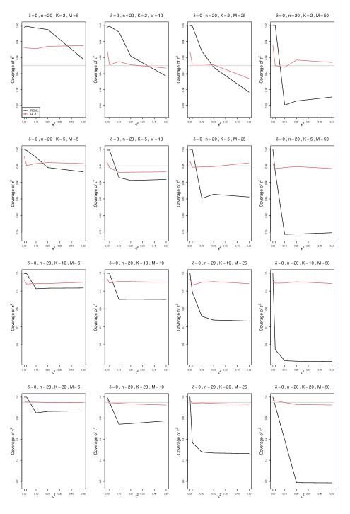
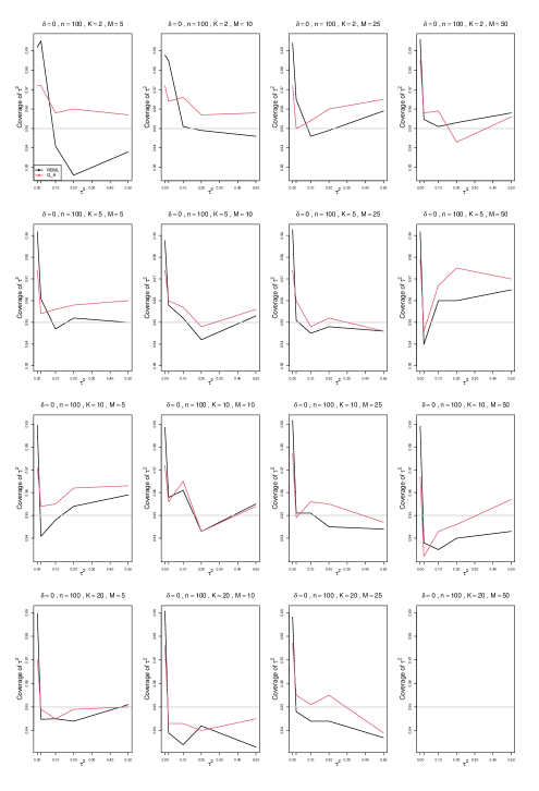
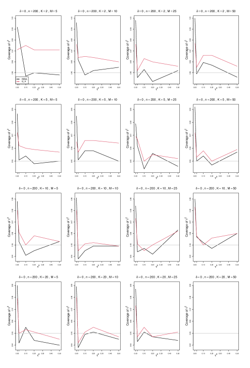
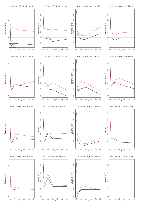
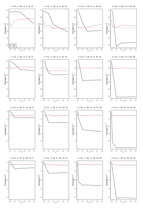
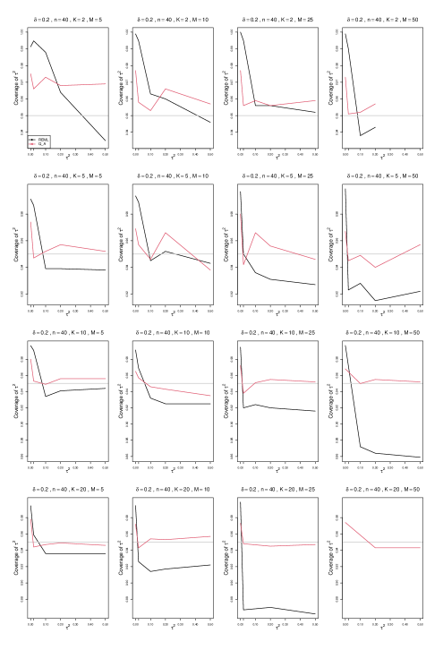
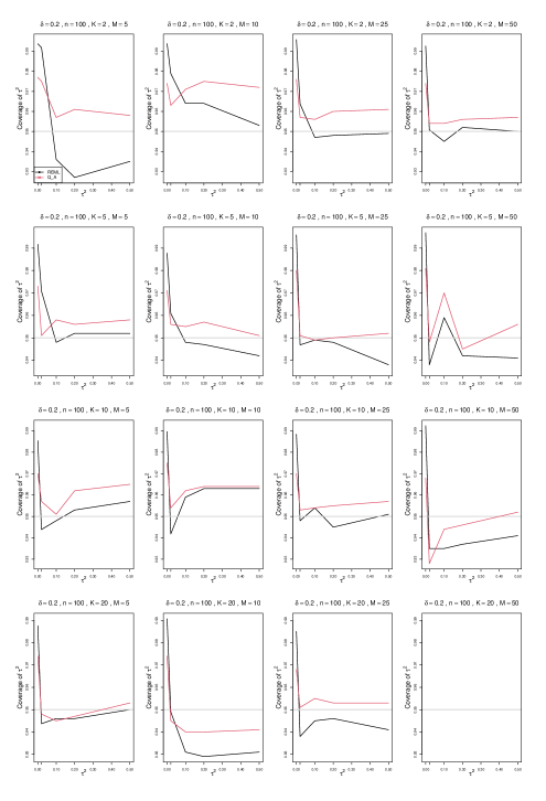
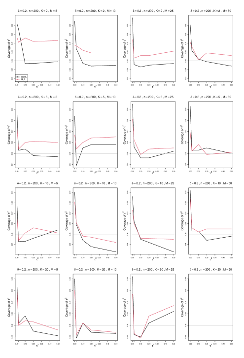
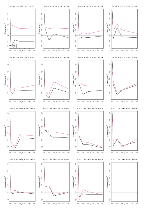
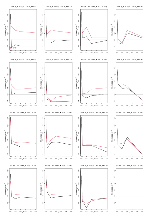
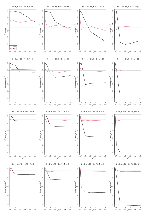
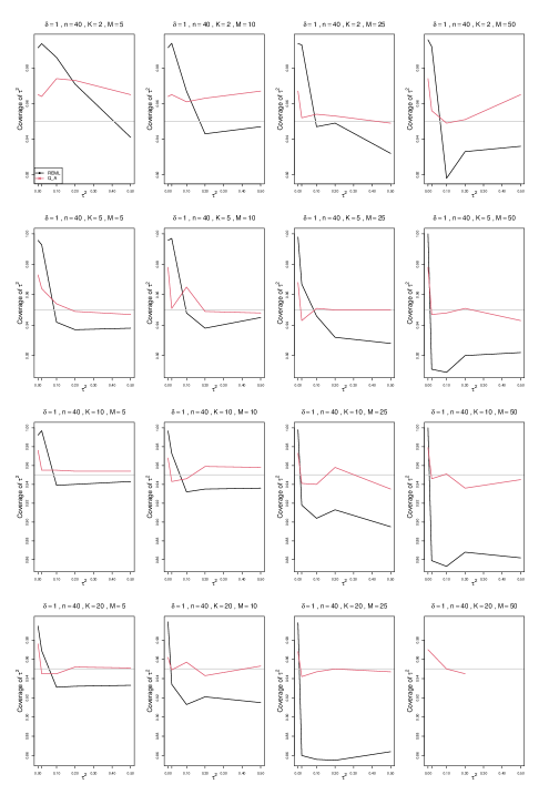
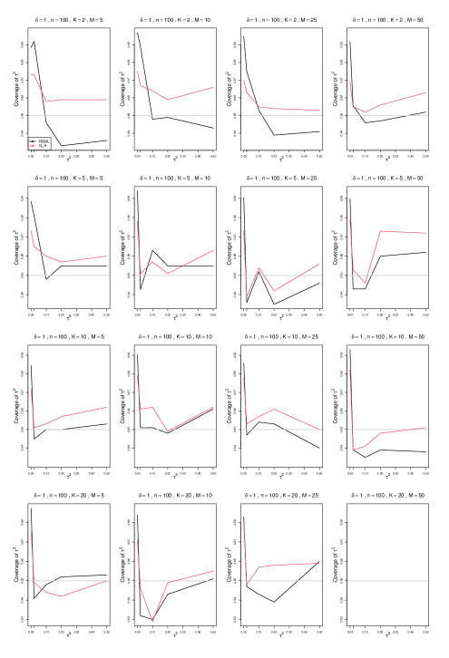
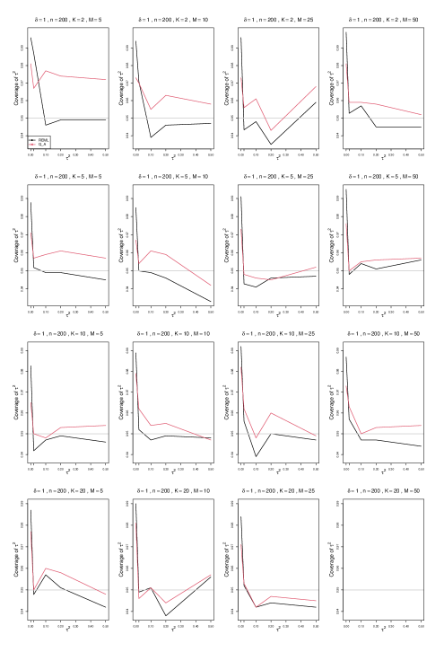
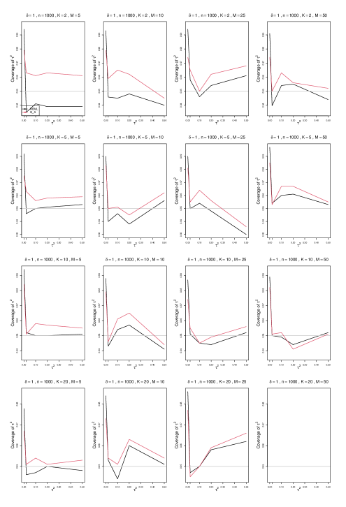
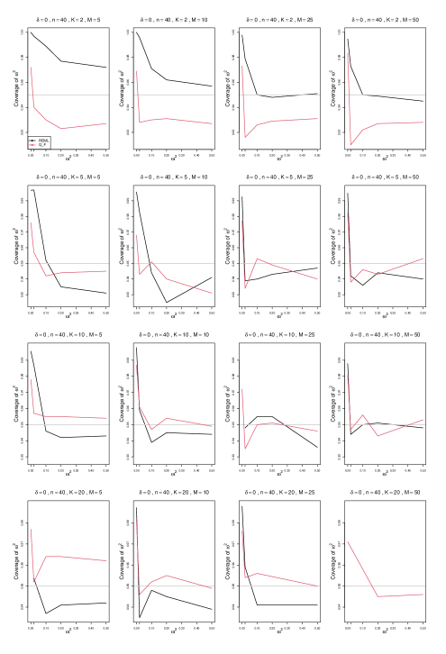
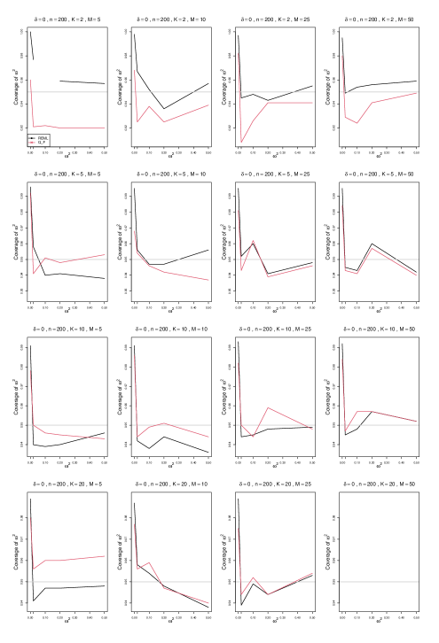
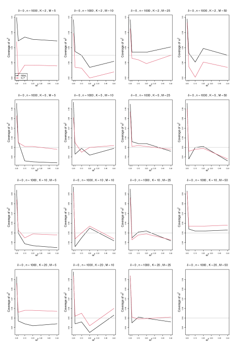
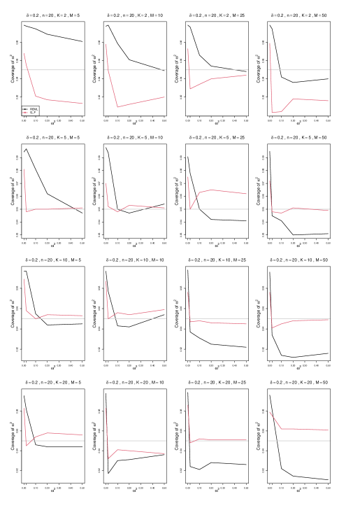
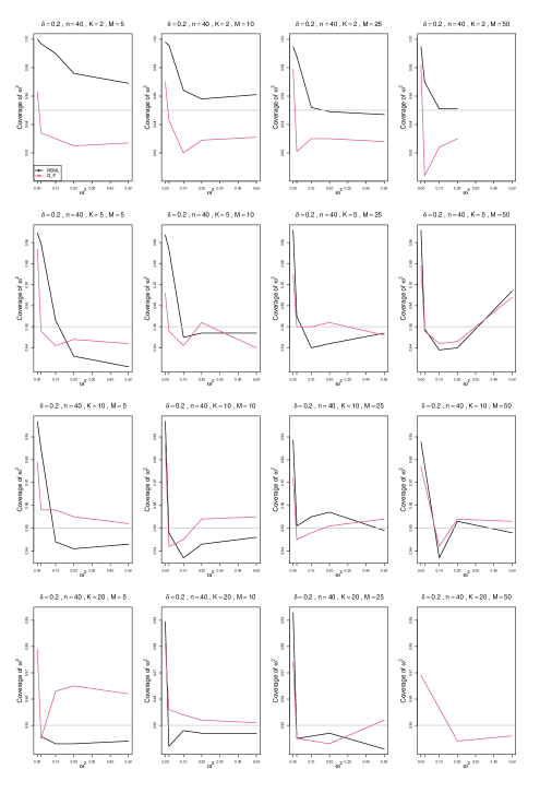
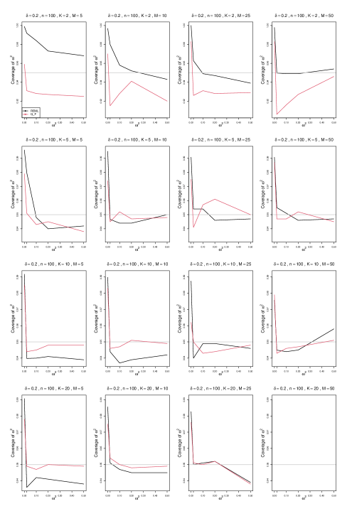
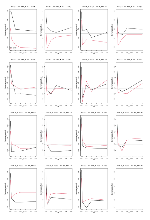
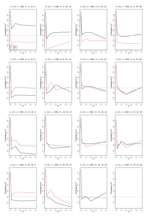
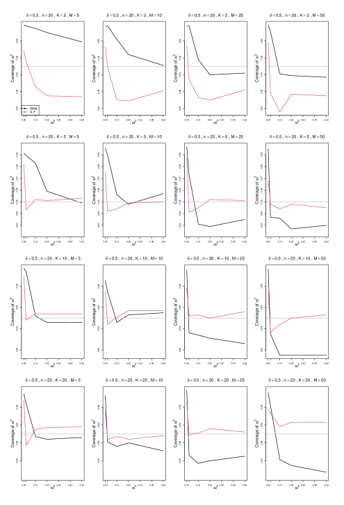
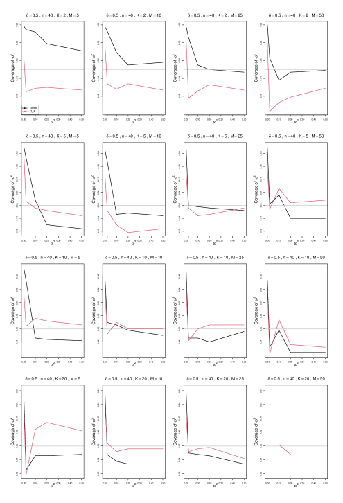
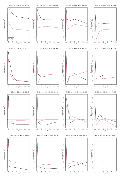
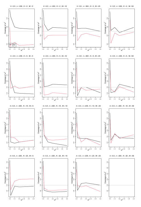
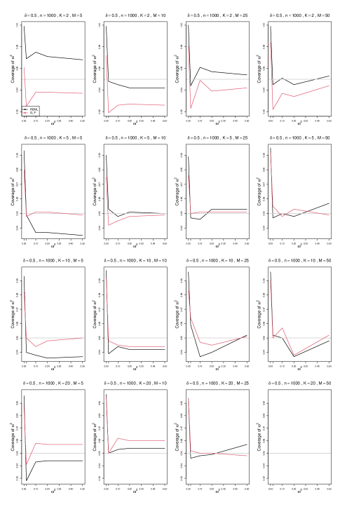
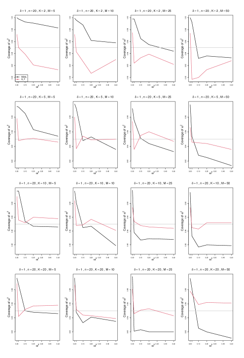
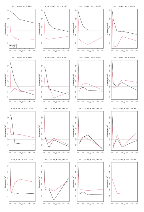
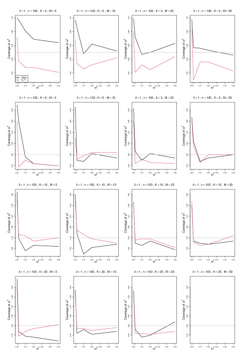
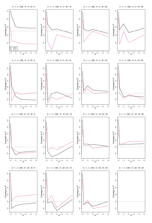
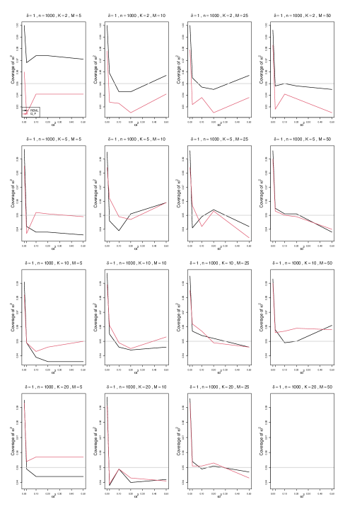
4.2.6 Coverage of interval estimators of (Appendix F)
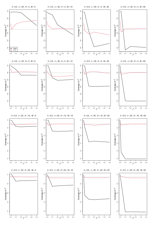
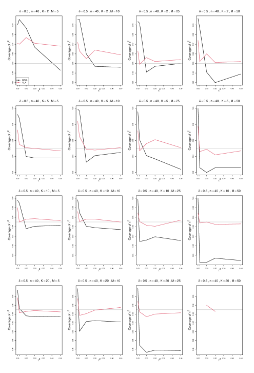
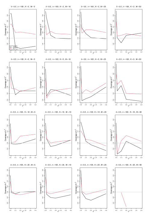
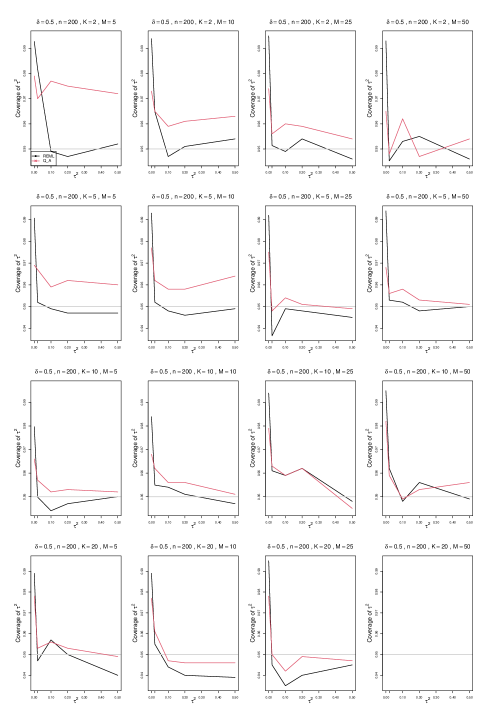
When and , -based intervals had lower than nominal coverage. The coverage of PL was too high at , but close to nominal otherwise. For , coverage of the -based intervals was somewhat high at and close to nominal for . The PL levels were higher at and close to nominal for , but too low for larger and ; for example, they were below 92% for and .
For , the patterns were similar, but the coverage of PL was sometimes lower, at 94%.
For , levels were too low for but were similar to and often better than PL for or . PL levels were close to nominal for .
The value of did not seem to affect coverage.
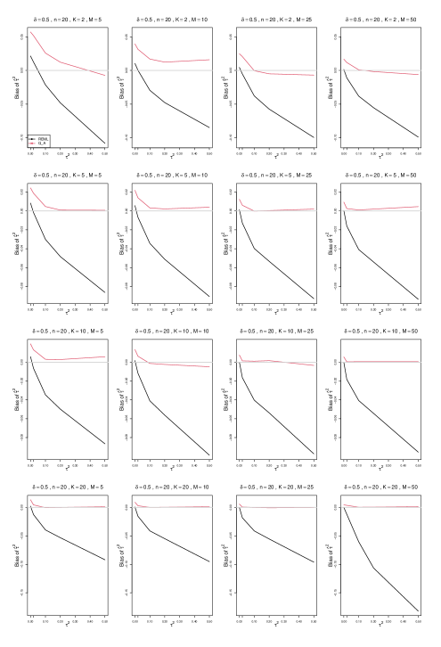
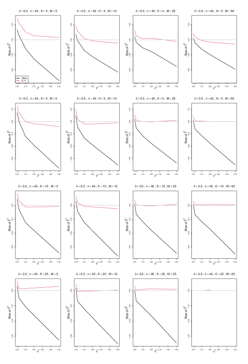
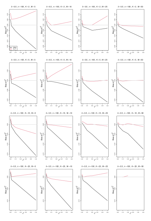
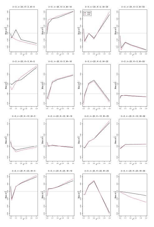
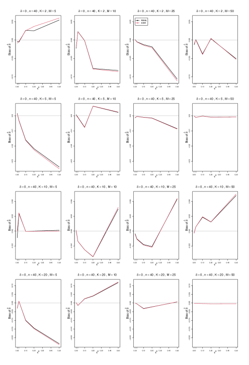
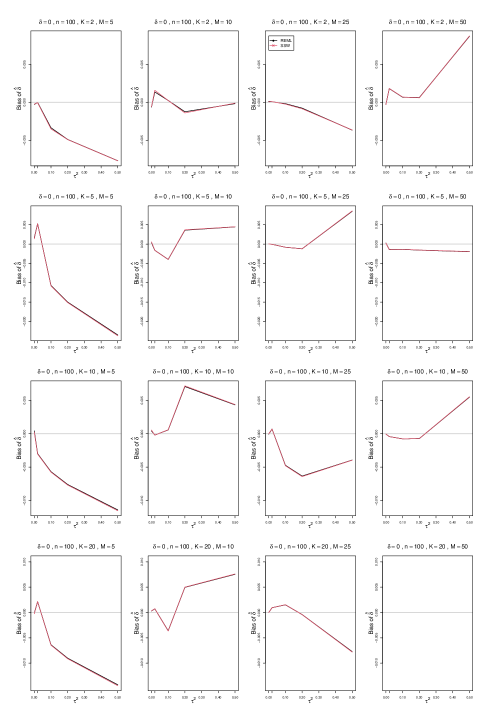
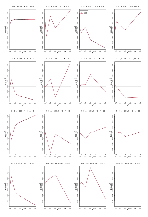
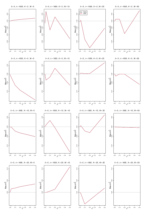
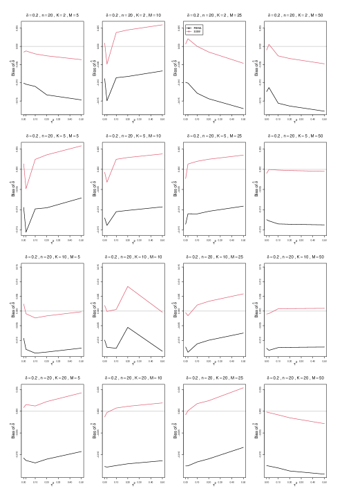
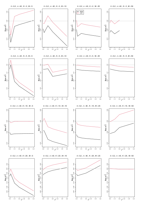
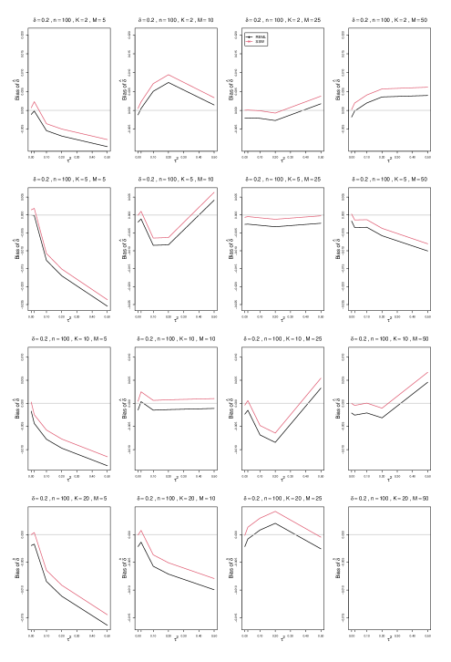
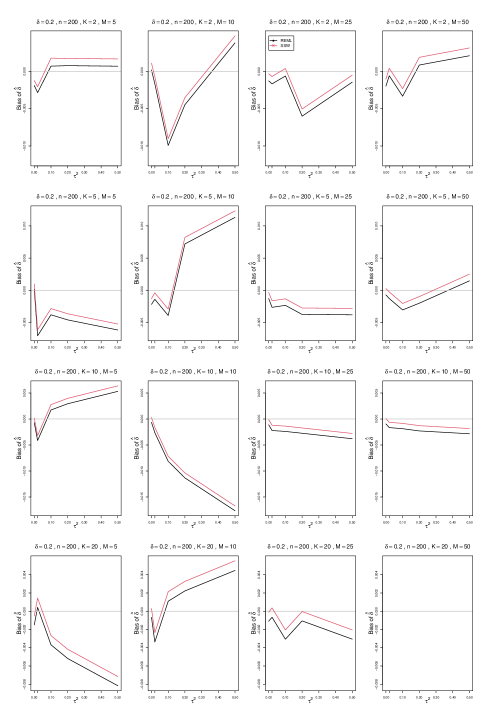
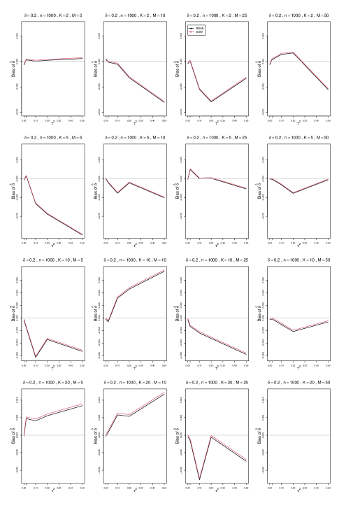
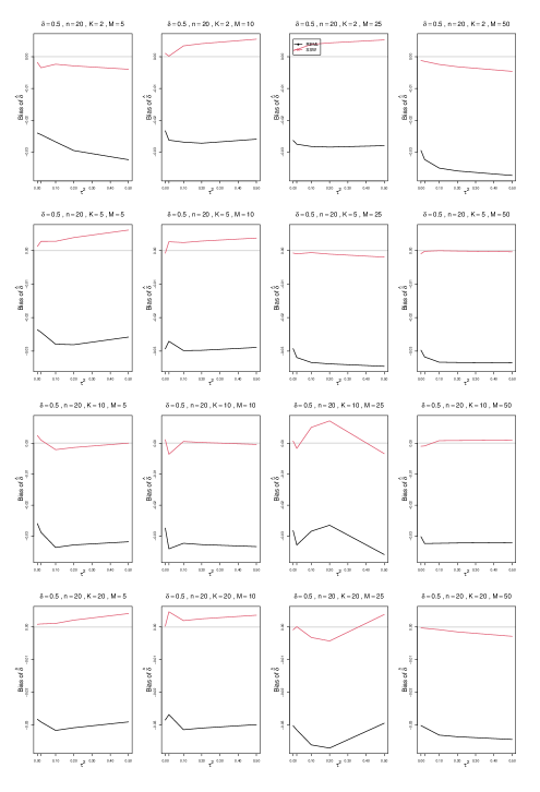
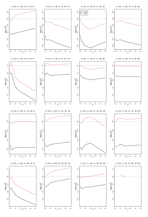
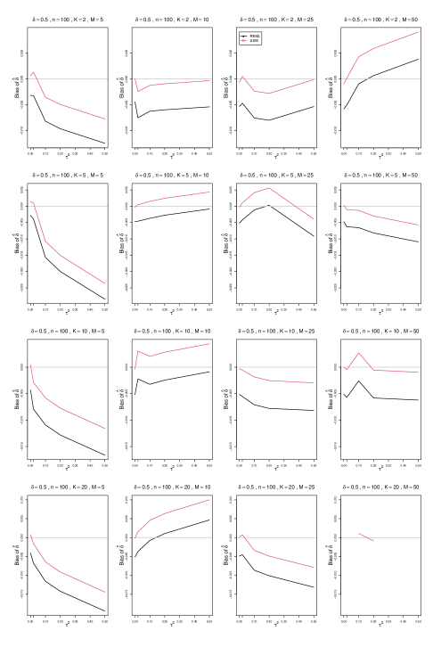
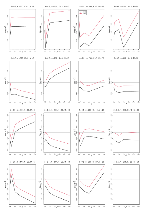
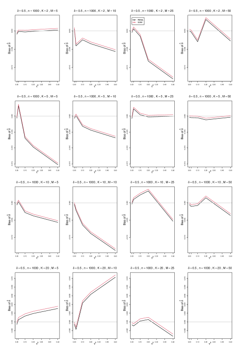
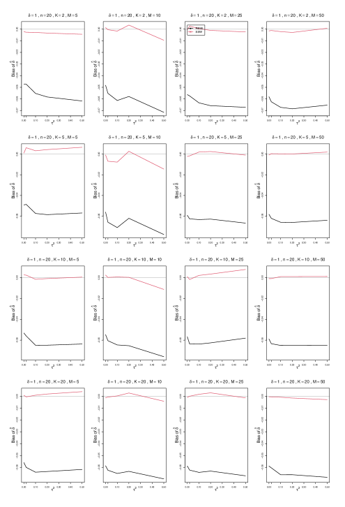
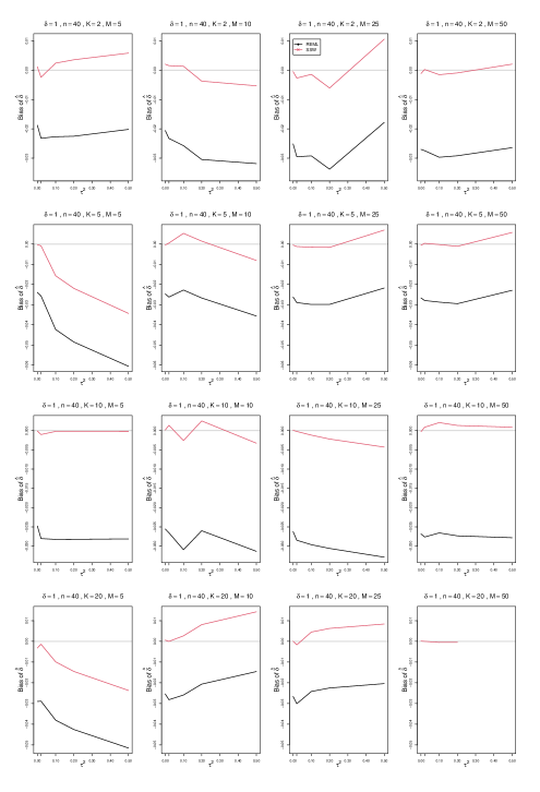
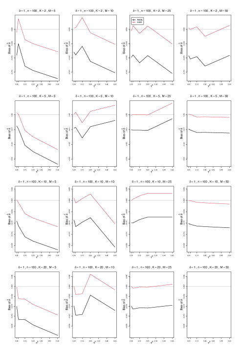
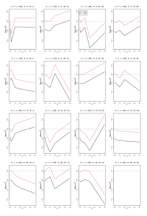
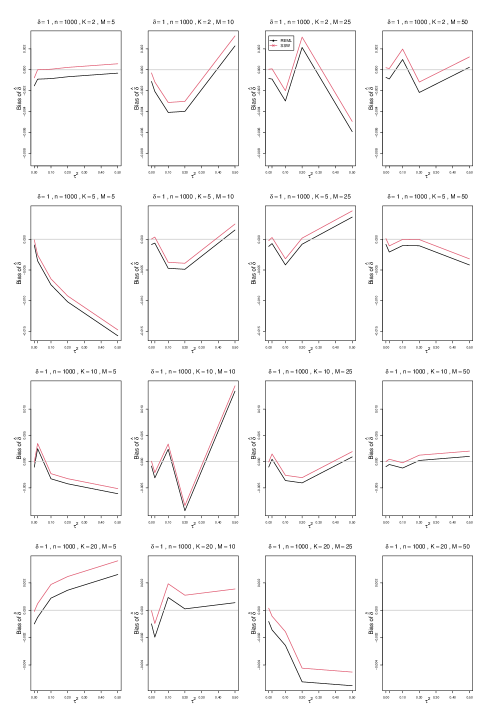
4.2.7 Bias of point estimators of (Appendix G)
The SSW estimator of was practically unbiased in all scenarios. The quality of the IV-based estimator was practically undistinguishable for .
The negative bias of the IV estimator increased noticeably with for larger values of , reaching about for and , regardless of and . This was due to increasing correlations between the estimators of and their IV weights. Typically, for each , a constant difference separated the two estimators for all and . Differences between the two estimators decreased with , almost disappearing by .
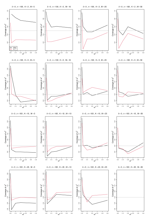
4.2.8 Coverage of interval estimators of (Appendix H)
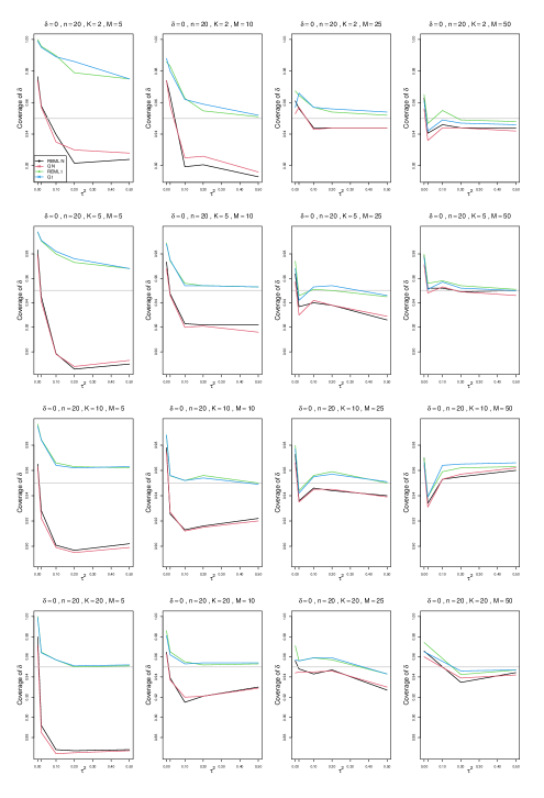
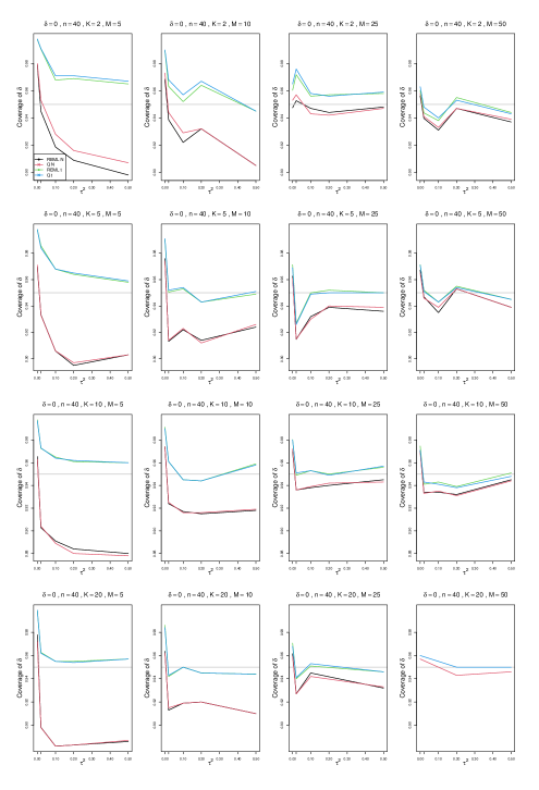
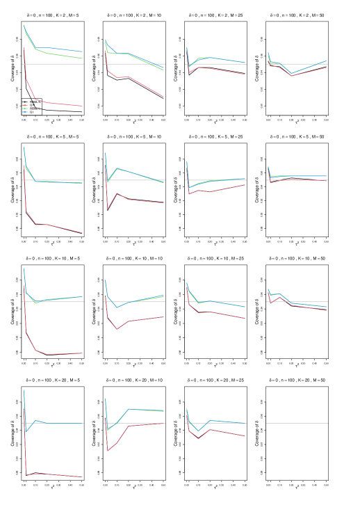
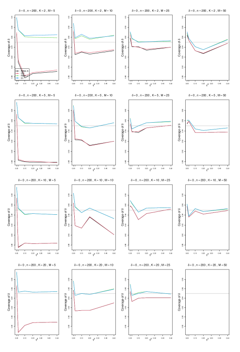
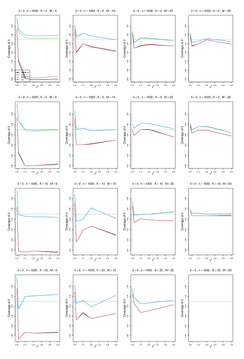
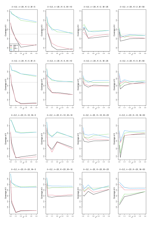
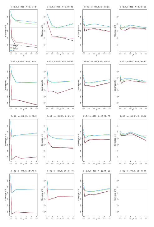
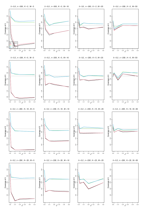
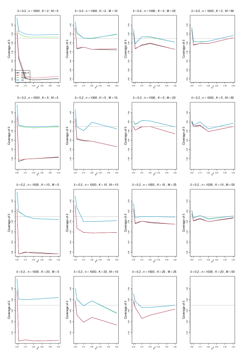
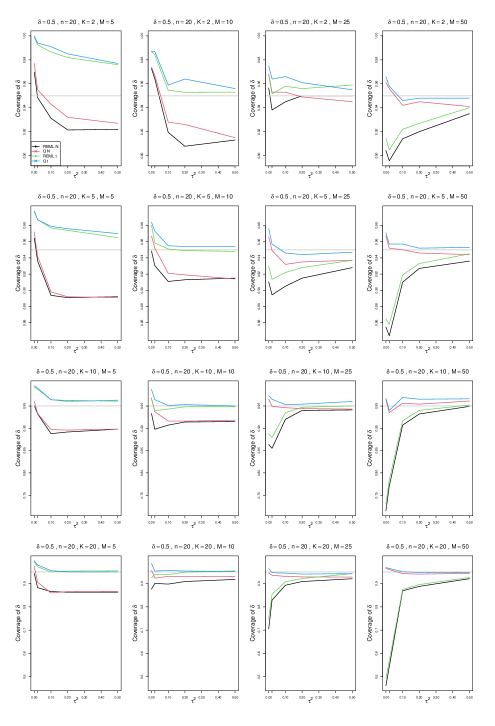
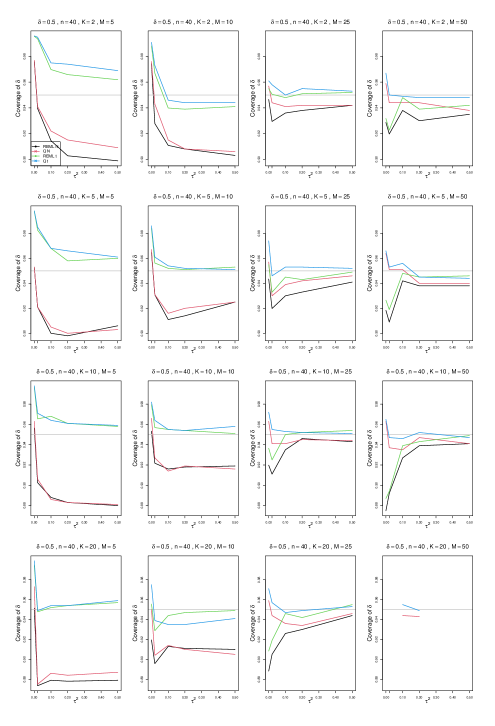
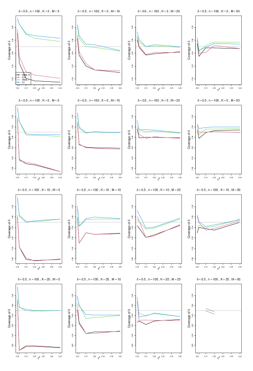
The source of critical values had a large impact. Except when , intervals that used normal critical values had coverage that was too low. The situation was especially acute for , where coverage was often below 90%. In contrast, intervals that used critical values had coverage close to 95% (but somewhat higher for ). The disparity was smaller when , and it generally shrank as increased.
The IV-based intervals showed considerable undercoverage for , , and larger . Larger was required to ameliorate this bias for larger in the vicinity of .
For , was problematic for , but coverage improved for larger . When , combinations of with were of concern. For , values of up to 200 produced undercoverage near .
5 Discussion
Multilevel meta-analysis is widely used in various applications. A need for three-level models arises especially often in social sciences and ecology. Examples include labs that each have several studies and studies that reported (mostly) the same set of outcome measures.
We propose a moment estimation approach similar to that in ANOVA, subdividing the total variation into within and between sums of squares. Importantly, we use fixed, effective-sample-size-based weights (SSW). The use of fixed weights allows separate estimation of meta-effects and variance components. This approach avoids convergence issues that require the standard methods to use iterative simultaneous estimation.
The model that we considered readily generalizes to handle cluster-specific between-study variances . For such a model, we would require separate statistics to estimate the values.
One can also consider more-complicated variance structures with . Then, similar to Jackson et al. [2024], we would need to estimate the covariance matrix from the residuals (Section 3.2), instead of using .
For the standardized mean difference as the effect measure, our simulation study compared our novel moment-based method of estimation in a three-level meta-analysis with the standard REML/PL-based methods of meta-analysis implemented in rma.mv in metafor. Overall, the new methods performed similarly to or better than the standard methods, and we recommend their use in practice.
An important observation is the unacceptably low coverage of the overall effect, regardless of the method used, by the standard confidence intervals based on normal critical values. A forceful warning about this shortcoming should be prominent in any meta-analysis software in which the -based intervals are not the default.
Acknowledgments
The work by E. Kulinskaya was supported by the Economic and Social Research Council [grant number ES/L011859/1].
References
- Cheung [2014] M. W.-L. Cheung. Modeling dependent effect sizes with three-level meta-analyses: A structural equation modeling approach. Psychological Methods, 19:211–229, 2014. doi: 10.1037/a0032968.
- Davies [1980] R. B. Davies. Algorithm AS 155: The distribution of a linear combination of random variables. Journal of the Royal Statistical Society Series C (Applied Statistics), 29:323–333, 1980. doi: 10.2307/2346911.
- DerSimonian and Kacker [2007] Rebecca DerSimonian and Raghu Kacker. Random-effects model for meta-analysis of clinical trials: an update. Contemporary Clinical Trials, 28(2):105–114, 2007. doi: 10.1016/j.cct.2006.04.004.
- Duchesne and de Micheaux [2010] P. Duchesne and P. Lafaye de Micheaux. Computing the distribution of quadratic forms: Further comparisons between the Liu-Tang-Zhang approximation and exact methods. Computational Statistics and Data Analysis, 54:858–862, 2010. doi: 10.1016/j.csda.2009.11.025.
- Farebrother [1984] R. W. Farebrother. Algorithm AS 204: The distribution of a positive linear combination of random variables. Journal of the Royal Statistical Society Series C (Applied Statistics), 33:332–339, 1984. doi: 10.2307/2347721.
- Fernández-Castilla et al. [2020] Belén Fernández-Castilla, Laleh Jamshidi, Lies Declercq, S. Natasha Beretvas, Patrick Onghena, and Wim Van den Noortgate. The application of meta-analytic (multi-level) models with multiple random effects: A systematic review. Behavior Research Methods, 52:2031–2052, 2020. doi: 10.3758/s13428-020-01373-9.
- Goldstein et al. [2000] Harvey Goldstein, Min Yang, Rumana Omar, Rebecca Turner, and Simon Thompson. Meta-analysis using multilevel models with an application to the study of class size effects. Journal of the Royal Statistical Society Series C (Applied Statistics), 49:399–412, 2000. doi: 10.1111/1467-9876.00200.
- Hardy and Thompson [1996] Rebecca J. Hardy and Simon G. Thompson. A likelihood approach to meta-analysis with random effects. Statistics in Medicine, 15(6):619–629, 1996. doi: 10.1002/(SICI)1097-0258(19960330)15:6¡619::AID-SIM188¿3.0.CO;2-A.
- Hedges [1983] Larry V. Hedges. A random effects model for effect sizes. Psychological Bulletin, 93(2):388–395, 1983. doi: 10.1037/0033-2909.93.2.388.
- Jackson et al. [2024] Dan Jackson, Wolfgang Viechtbauer, and Robbie C. M. van Aert. Multistep estimators of the between-study covariance matrix under the multivariate random-effects model for meta-analysis. Statistics in Medicine, 43(4):756–773, 2024. doi: 10.1002/sim.9985.
- Konstantopoulos [2011] Spyros Konstantopoulos. Fixed effects and variance components estimation in three-level meta-analysis. Research Synthesis Methods, 2(1):61–76, 2011. doi: 10.1002/jrsm.35.
- R Core Team [2016] R Core Team. R: A Language and Environment for Statistical Computing. R Foundation for Statistical Computing, Vienna, Austria, 2016. URL https://www.R-project.org/.
- Raudenbush and Bryk [1985] S. W. Raudenbush and A. S. Bryk. Empirical Bayes meta-analysis. Journal of Educational Statistics, 10(2):75–98, 1985. doi: 10.2307/1164836.
- Viechtbauer [2010] Wolfgang Viechtbauer. Conducting meta-analyses in R with the metafor package. Journal of Statistical Software, 36:3, 2010. doi: 10.18637/jss.v036.i03. Website: https://www.metafor-project.org.
Appendices
-
•
Appendix A: Rate of non-convergence for the default rma.mv REML-based analysis
-
•
Appendix B: Empirical level of the two tests, at , for heterogeneity of SMD
-
•
Appendix C: Bias in point estimators of the between-study variance
-
•
Appendix D: Coverage of 95% confidence intervals for the between-study variance
-
•
Appendix E: Bias in point estimators of the between-cluster variance
-
•
Appendix F: Coverage of 95% confidence intervals for the between-cluster variance
-
•
Appendix G: Bias in point estimators of the overall effect
-
•
Appendix H: Coverage of 95% confidence intervals for the overall effect
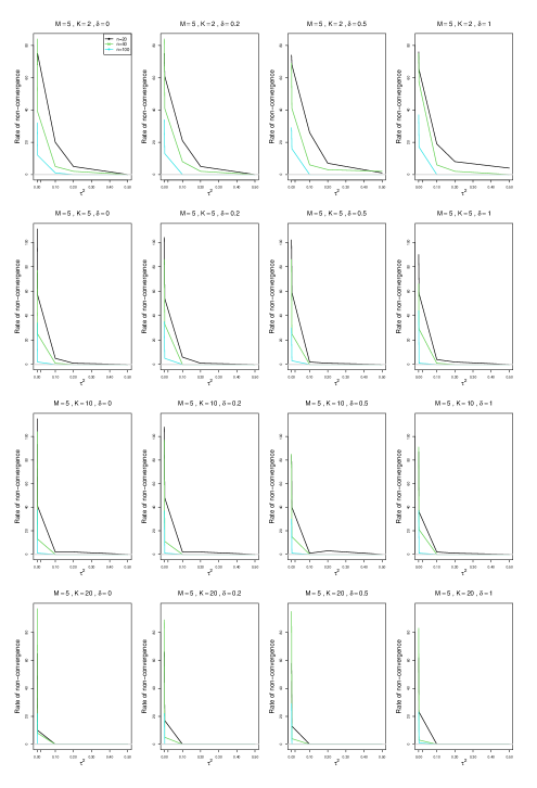
Appendix A: Rate of non-convergence for the default rma.mv REML-based analysis
Each figure corresponds to a value of the number of clusters ( = 5, 10, 25, 50).
For each combination of the number of studies in a cluster ( = 2, 5, 10, 20) and the standardized mean difference ( = 0, 0.2, 0.5, 1), a panel plots (versus = 0, 0.02, 0.1, 0.2, 0.5) the rate of non-convergence for the rma.mv-based analysis.
The traces in the plot correspond to , , and .
Appendix B: Empirical level of the two tests, at , for heterogeneity of SMD
Each figure corresponds to a value of the standardized mean difference ( = 0, 0.2, 0.5, 1).
For each combination of the number of studies in a cluster ( = 2, 5, 10, 20) and the number of clusters ( = 5, 10, 25, 50), a panel plots the empirical level of the tests (at the .05 level) versus (= 20, 40, 100, 200, 1000) for Davies’s approximations to null distributions of and , which use effective-sample-size weights.
Appendix C: Bias in point estimators of the between-study variance
Each figure corresponds to a value of the standardized mean difference ( = 0, 0.2, 0.5, 1) and a value of the study sample size ( = 20, 40, 100, 200, 1000).
For each combination of the number of studies in a cluster ( = 2, 5, 10, 20) and the number of clusters ( = 5, 10, 25, 50), a panel plots bias versus (= 0, 0.02, 0.1, 0.2, 0.5).
The two variance components are held equal ().
The point estimators of are
-
•
REML method, inverse-variance weights, rma.mv in metafor
-
•
(conditional moment-based method, effective-sample-size weights)
Appendix D: Coverage of 95% confidence intervals for the between-study variance
Each figure corresponds to a value of the standardized mean difference ( = 0, 0.2, 0.5, 1) and a value of the study sample size ( = 20, 40, 100, 200, 1000).
For each combination of the number of studies in a cluster ( = 2, 5, 10, 20) and the number of clusters ( = 5, 10, 25, 50), a panel plots coverage of versus (= 0, 0.02, 0.1, 0.2, 0.5).
The two variance components are held equal ().
The interval estimators of are
-
•
PL (Profile-Likelihood method, inverse-variance weights, rma.mv in metafor)
-
•
(conditional moment-based method, effective-sample-size weights, Davies’s approximation to the distribution)

Appendix E: Bias in point estimators of the between-cluster variance
Each figure corresponds to a value of the standardized mean difference ( = 0, 0.2, 0.5, 1) and a value of the study sample size ( = 20, 40, 100, 200, 1000).
For each combination of the number of studies in a cluster ( = 2, 5, 10, 20) and the number of clusters ( = 5, 10, 25, 50), a panel plots bias versus (= 0, 0.02, 0.1, 0.2, 0.5).
The two variance components are held equal ().
The point estimators of are
-
•
REML method, inverse-variance weights, rma.mv in metafor)
-
•
(conditional moment-based method, effective-sample-size weights)

Appendix F: Coverage of 95% confidence intervals for the between-cluster variance
Each figure corresponds to a value of the standardized mean difference ( = 0, 0.2, 0.5, 1) and a value of the study sample size ( = 20, 40, 100, 200, 1000).
For each combination of the number of studies in a cluster ( = 2, 5, 10, 20) and the number of clusters ( = 5, 10, 25, 50), a panel plots coverage of at the 95% nominal level versus (= 0, 0.02, 0.1, 0.2, 0.5).
The two variance components are held equal ().
The interval estimators of are
-
•
PL (Profile-Likelihood method, inverse-variance weights, rma.mv in metafor)
-
•
(conditional moment-based method, effective-sample-size weights, Davies’s approximation to the distribution)
Appendix G: Bias in point estimation of the overall effect
Each figure corresponds to a value of the standardized mean difference ( = 0, 0.2, 0.5, 1) and a value of the study sample size ( = 20, 40, 100, 200, 1000).
For each combination of the number of studies in a cluster ( = 2, 5, 10, 20) and the number of clusters ( = 5, 10, 25, 50), a panel plots bias of versus (= 0, 0.02, 0.1, 0.2, 0.5).
The two variance components are held equal ().
The point estimators of are
-
•
REML method, inverse-variance weights, rma.mv in metafor)
-
•
SSW (conditional moment-based method, effective-sample-size weights)
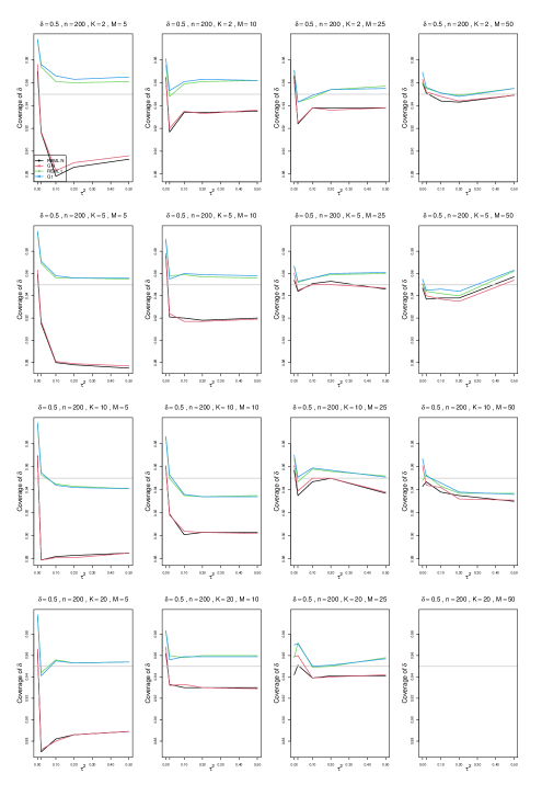
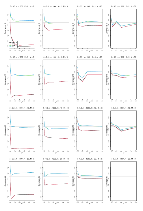
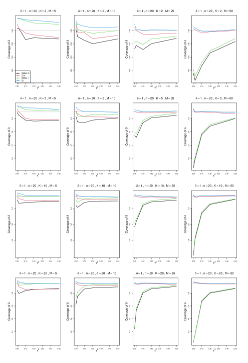
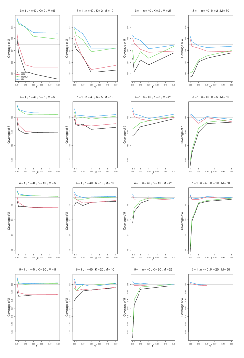
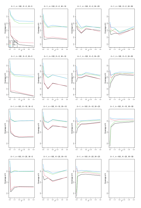
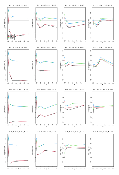
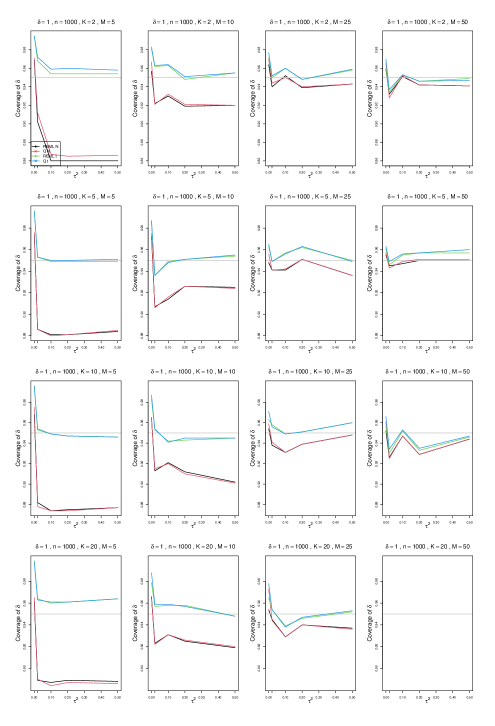
Appendix H: Coverage of 95% confidence intervals for the overall effect
Each figure corresponds to a value of the standardized mean difference ( = 0, 0.2, 0.5, 1) and a value of the study sample size ( = 20, 40, 100, 200, 1000).
The two variance components are held equal ().
For each combination of the number of studies in a cluster ( = 2, 5, 10, 20) and the number of clusters ( = 5, 10, 25, 50), a panel plots coverage of the overall effect at the 95% nominal level versus (= 0, 0.02, 0.1, 0.2, 0.5).
The interval estimators of are centered at a point estimator of . Their half-width equals the point estimator’s standard error, calculated from REML or from moment-based estimators of variance components, combined with normal or critical values.
-
•
REML N (REML, inverse-variance weights, normal critical values rma.mv in metafor)
-
•
REML t (REML, inverse-variance weights, critical values rma.mv in metafor)
-
•
N (conditional moment-based method, effective-sample-size weights, normal critical values)
-
•
t (conditional moment-based method, effective-sample-size weights, critical values)