Erlang Model for Multiple Data Streams

Abstract

With the development of information technology, requirements for data flow have become diverse. When multiple data streams (MDS) are used, the demands of users change over time, which makes traditional teletraffic analysis not directly applicable. This paper proposes probabilistic models for the demand of MDS services, and analyzes in three states: non-tolerance, tolerance and delay. When the requirement random variables are co-distributed with respect to time, we rigorously prove the practicability of the Erlang Multirate Loss Model (EMLM) from a mathematical perspective by discretizing time and error analysis. An algorithm of pre-allocating resources for communication society is given to guild the construction of base resources.

I Introduction

Communication has become an indispensable part of modern society. For a community, a large number of users will make communication requirements at the same time, and each requirement needs to allocate communication resources, such as telephone lines, time-frequency resource grids, etc. When infrastructure construction is carried out (such as base stations), if there are few preset communication resources, the user demand in the area will be frequently blocked, resulting in a poor user experience, while too many preset resources will lead to increased costs and waste. Therefore, predicting the performance of users’ requirements in the communication society and selecting reasonable resource presets are important steps in infrastructure construction[1].

In 1917, A.K. Erlang obtained his famous formula from the analysis of the statistical equilibrium and laid the foundations of modern teletraffic theory[2]. By modeling the number of arrival users as Poisson random variable and the required time being exponential distributed, Erlang formula can deduce the blocking probability for telephone communication, according to the birth and death process theory.

The original Erlang model was only for telephone line, however, with the development of wireless communication, modern forms of communication continued to evolve and expand. Particularly, after the popularization of 5G, users’ requirements have become rich and diverse, including calls, text messages, voice, games, videos, short videos, etc., and we call these multiple needs as multiple data streams (MDS). Clearly, each of requirements has its own characteristics. For example, the traditional communication method of telephone, which presents a stable demand, while the requirement for games or short videos is rapidly changing. Therefore, traditional models are clearly not sufficient to describe modern communication needs.

In order to be suitable with complex situations, Erlang formula has been sustainably developing. [3] considered two types of requirements, narrow-band and wide-band, and calculate the related blocking probability, in 1965. With more analysis, the number of types can be generated to any integer $K$ and the model was called as Eralng Multirate Loss Model (EMLM) [4]. Some specific policies on link, waiting or tolerance were also added in the model to meet several situations [4], [5], [6]. There are also some works on the assumptions of the arrival user and required time. [7] studied the case when the size of community is not large enough, and used quasi-random call arrival process to replace Poisson arrival process. In addition, the loss was thought as the noise when the band-demand exceeded the total band. [8] set two stages for activated users: ON and OFF. When an user is ON, he requires $b_{k}$ band if he is in class $k$, and when he finishes the stage ON, he becomes OFF with probability $\sigma_{k}$ and leaves with probability $1-\sigma_{k}$. When an user finishes his OFF stage, he ask to become ON. This assumption is called as ON-OFF model, which was enhanced for finite population community [1]. An Erlang model with varied cost in time was studied in [9].

However, different with classical teletraffic situation, MDS implies a queue problem for users with random number of services for a certain time. Existing models are still not able to describe the MDS accurately since the requirement varies with time. Therefore, this paper establishes the probability models and Erlang formulas for MDS. We denote the requirements of user $i$ at time $t$ as $X_{i}(t)$ (can be different for different $i$ and $t$). In Section II, we consider that the requirement depends on the time of demand duration, and build probability models in three cases, non-tolerance, instant tolerance and delay. After assuming $X_{i}(t)$s are i.i.d. with respect to $i$ and $t$ with finite support set, Erlang formula is introduced in Section III. By discrete-time analysis, we find that the stable distribution of requirement is the same whatever $X_{i}(t)$s are variable or invariable with $t$. Therefore, we can solve the stable distribution of requirement for MDS by EMLM. A ON-OFF model is also discussed in Section III. The algorithm for pre-allocating TF resources and example are shown in Section IV, and we conclude our results in Section V. The main contributions of this paper are summarized as follows.

1. For the case that requirements $X_{i}(t)$s depend on the time of demand duration, we build probability models for MDS in three cases, non-tolerance, instant tolerance and delay, and obtain the blocking probability.

2. Since the requirements of MDS are time-variable, we apply the discretization for time in order to describe the distribution of total requirement. By error analysis, we find that the stable distribution of requirement is the same whatever $X_{i}(t)$s are variable or invariable with $t$. Thus we conclude that EMLM can be still used for MDS.

3. The algorithm for pre-allocating resources is designed to guild the construction of base stations.

Some notations are organized here. $X_{i}(t)$ denotes the requirement of user $i$ at time $t$, $A(t)$ denotes the activated users at time $t$ and $|A(t)|$ denotes its number. We use $Poi(\lambda)$ and $E(\mu)$ to imply the random variables having Poisson distribution with rate $\lambda$ and exponential distribution with rate $\mu$ respectively, and $a\sim A$ means the random variable $a$ obeys the distribution $A$. We use $(\cdot)^{k}$ to represent the $k$ Cartesian product. $N$ always means the total number of users in a community while $C$ denotes the total number of resources. In the following of this paper, we consider a community with $N$ potential users for MDS.

II Probability Models for Time-dependent MDS

Since the arrival of users for MDS are not significantly different with classical teletraffic problem, we still assume that the arrived number of users $I(t)$ follows a Poisson distribution with rate $\lambda N$, i.e. $I(t)\sim Poi(\lambda N),\forall t$. In order to simplify the model, we assume that the serving time is discrete and there is an uniformly bound for single use-time as $T$, since in a colorful life, we have a lot more to do than using the internet. This assumption also does not contradict with exponential distributed demand time in classical Erlang model since we can set the unit to be small enough to be close to continuous time, and the probability of required time exceeding a large number $T$ is almost vanished. Note that if an user $i$ needs a $T_{0}(<T)$ demand duration, then we have $X_{i}(t)=0,\tau_{i}+T_{0}<t<\tau_{i}+T$, where $\tau_{i}$ is the demand start time of user $i$ and $t-\tau_{i}$ has uniformly distribution on $[T]:=\{0,1,\cdots,T\}$.

It is apparently that the main different of different users are their start time $\tau_{i}$s, thus we assume that all activated users asking requirement with a same distribution family $\{W(s),s\in\{0,1,2,\cdots,T\}\}$, i.e. $X_{i}(t)\sim W(t-\tau_{i}),i=1,2,\cdots,|A(t)|$.

Given $C$ unit resources serving for a community, we set standard to assess traffic overload.

1. Non-tolerance. It implies that blockage occurs when demand exceeds total resources, i.e.

   $$\frac{C}{\sum_{i\in A(t)}X_{i}(t)}\geq 1.$$ (1)

2. Tolerance with threshold $\alpha\in(0,1)$. It means that a small amount of distortion is allowed. When demand exceeds resources, the data stream is compressed (such as reducing image or sound quality) to ensure smooth transmission. This is a very common method, and the maximum acceptable compression rate is set to be $1-\alpha$. Thus the blockage happens when

   $$\frac{C}{\sum_{i\in A(t)}X_{i}(t)}\geq\alpha.$$ (2)

3. Loss as delay. In this case, the un-transmitted information may be also put in the requirement in the next transmit-time, together with the new demands.

II-A Non-tolerance

Under the above settings, it is clear that at time $t$, there are $I(t-T-1)$ users finishing their requirements, and $I(t)$ users joining in, thus when $t$ is large enough,

$$|A(t)|=|A(t-1)|+I(t)-I(t-T-1)\overset{d}{=}\sum_{i=0}^{T}I(i),$$ (3)

where $I(t)\sim Poi(\lambda N)$, and $\overset{d}{=}$ means equal in distribution. Note that $I(t)$ is independent of $A(t-1)$ and $I(t-T)$, thus the blocking probability is

$$\mathbb{P}\left(\frac{Cf}{\sum_{i\in A(t)}X_{i}(t)}<1\right)$$ (4)

$$=\sum_{k=1}^{\infty}\mathbb{P}(|A(t)|=k)\sum_{t^{k}-\vec{t}\in[T]^{k}}\frac{1}{(T+1)^{k}}\mathbb{P}\left(\sum_{i=1}^{k}W_{i}(t-t_{i})>C\right),$$ (5)

where $W_{i}(t)\sim W(t)$ are independent, $t^{k}=(t,t,\cdots,t)_{1\times k},\vec{t}=(t_{1},t_{2},\cdots,t_{k})$.

By the property of Poisson process, $|A(t)|\sim Poi(\lambda N(T+1))$, thus

$$\mathbb{P}\left(\frac{C}{\sum_{i\in A(t)}X_{i}(t)}<1\right)$$ (6)

$$=\sum_{k=1}^{\infty}\frac{(\lambda N)^{k}}{k!}e^{-\lambda N(T+1)}\sum_{\vec{t}\in[T]^{k}}\mathbb{P}\left(\sum_{i=1}^{k}W_{i}(t_{i})>C\right).$$

Since the distributions of family $\{W(s),s\in\{0,1,2,\cdots,T\}\}$ are known (estimated by sampling for example), the blocking probability is obtained by (6).

II-B Tolerance

It is obvious that tolerance case (2) is similar with non-tolerance (1) by replacing $C$ to $C/\alpha$, thus the blocking probability can be deduced directly that

$$\mathbb{P}\left(\frac{C}{\sum_{i\in A(t)}X_{i}(t)}<\alpha\right)$$ (7)

$$=\sum_{k=1}^{\infty}\frac{(\lambda N)^{k}}{k!}e^{-\lambda N(T+1)}\sum_{\vec{t}\in[T]^{k}}\mathbb{P}\left(\sum_{i=1}^{k}W_{i}(t_{i})>\frac{C}{\alpha}\right).$$

II-C Delay

When the demand at a certain moment exceeds the amount of resources, the users will allocate the resources proportionally according to their requirements, and the remaining demand will be added to the demand of the next unit of time, i.e., a (proportional) delay occurs. We denote the total requirements (arrival and delay) of user $i$ at time $t$ as $Y_{i}(t)$. Clearly, $Y_{i}$ does not have the same distribution as $X_{i}$. But $Y_{i}$s are still i.i.d., in fact $Y_{i}(\tau_{i})=X_{i}(\tau_{i})$, and when $\tau_{i}+1\leq t\leq\tau_{i}+T$,

$$Y_{i}(t)-X_{i}(t)$$

$$=Y_{i}(t-1)\max\left\{\left(1-\frac{C}{\sum_{j\in A(t-1)}Y_{j}(t-1)}\right),0\right\},$$

Replace $X_{i}$ by $Y_{i}$ in (7), we can obtain the target probability for delay case. Note that $Y$ may not easily sampled as $X$, but if we denote $S(t)=\sum_{i\in A(t)}Y_{i}(t)$, we have

$$S(t)= \max\{0,S(t-1)-C\}+\sum_{i\in A(t)}X_{i}(t)$$ (8)

$$=\max\{0,S(t-1)-C\}+\sum_{i\in A(t)}W_{i}(t-\tau_{i})$$

$$\overset{\Delta}{=}S(t,\tau_{1},\tau_{2},\cdots,\tau_{|A(t)|}),$$

and the blocking probability becomes

$$\mathbb{P}\left(\frac{C}{\sum_{i\in A(t)}Y_{i}(t)}\leq\alpha\right)=\mathbb{P}\left(\frac{C}{S(t)}\leq\alpha\right)$$ (9)

$$=\sum_{k=1}^{\infty}\mathbb{P}(|A(t)|=k)\sum_{\vec{t}\in[T]^{k}}\frac{1}{(T+1)^{k}}\mathbb{P}\left(S(t,\vec{\tau}=\vec{t})>\frac{C}{\alpha}\right)$$

$$=\sum_{k=1}^{\infty}\frac{(\lambda N)^{k}}{k!}e^{-\lambda N(T+1)}\sum_{\vec{t}\in[T]^{k}}\mathbb{P}\left(S(t,\vec{\tau}=\vec{t})>\frac{C}{\alpha}\right).$$

In order to estimated the distribution of $S(t)$, we assume that the requirements are discrete (integers), which is applied in practice. Then the blocking probability can be write as (10).

$$\mathbb{P}\left(\frac{C}{S(t)}\leq\alpha\right) =\sum_{k=1}^{\infty}\sum_{l=0}^{k}\mathbb{P}(I(t)=l)\mathbb{P}\left(\sum_{i=t-T}^{t-1}I(i)=k-l\right)C_{k}^{l}\sum_{\vec{t}\in([T]\setminus 0)^{k-l}}\frac{1}{T^{k-l}}\mathbb{P}(S(t,(0^{l},t_{1},t_{2},\cdots,t_{k-l}))>\frac{C}{\alpha})$$ (10)

$$=\sum_{k=1}^{\infty}\sum_{l=0}^{k}\mathbb{P}(I(t)=l)\mathbb{P}\left(\sum_{i=t-T}^{t-1}I(i)=k-l\right)C_{k}^{l}\sum_{\vec{t}\in([T]\setminus 0)^{k-l}}\frac{1}{T^{k-l}}\sum_{i=\lceil\frac{C}{\alpha}\rceil}^{P}\mathbb{P}(S(t,(0^{l},t_{1},t_{2},\cdots,t_{k-l}))=i)$$

$$=\sum_{k=1}^{\infty}\sum_{l=0}^{k}C_{k}^{l}e^{-\lambda N(T+1)}\frac{(\lambda N)^{k}}{l!(k-l)!}\sum_{\vec{t}\in([T]\setminus 0)^{k-l}}\sum_{i=\lceil\frac{C}{\alpha}\rceil}^{P}\mathbb{P}(S(t,(0^{l},t_{1},t_{2},\cdots,t_{k-l}))=i).$$

The only unknown term is $\mathbb{P}(S(t,(0^{l},t_{1},t_{2},\cdots,t_{m})=i))$, it may obtained by recursion as shown in (11).

$$\mathbb{P}(S(t,(0^{l},t_{1},t_{2},\cdots,t_{m})=i))$$ (11)

$$=\sum_{j=0}^{\infty}\mathbb{P}(I(t-T-1)=j)\sum_{a=0}^{P}\mathbb{P}(S(t-1,(T^{j},t_{1}-1,t_{2}-1\cdots,t_{m}-1))=a)$$

$$\;\;\;\;\cdot\mathbb{P}\left(S(t,(0^{l},t_{1},t_{2}\cdots,t_{m}))=i|S(t-1,(T^{j},t_{1}-1,t_{2}-1\cdots,t_{m}-1))=a\right)$$

$$=\sum_{j=0}^{\infty}\mathbb{P}(I(t-T-1)=j)\sum_{a=0}^{P}\mathbb{P}(S(t-1,(T^{j},t_{1}-1,t_{2}-1\cdots,t_{m}-1))=a)\mathbb{P}\left(\sum_{k=1}^{l}W_{k}(0)+\sum_{k=1}^{m}W_{k}(t_{k})=i-\max\{0,a-C\}\right)$$

$$=\sum_{j=0}^{\infty}e^{-\lambda N}\frac{(\lambda N)^{j}}{j!}\sum_{a=0}^{P}\mathbb{P}(S(t-1,(T^{j},t_{1}-1,t_{2}-1\cdots,t_{m}-1))=a)\mathbb{P}\left(\sum_{k=1}^{l}W_{k}(0)+\sum_{k=1}^{m}W_{k}(t_{k})=i-\max\{0,a-C\}\right)$$

The calculation of $\mathbb{P}\left(\sum_{k=1}^{l}W_{k}(0)+\sum_{k=1}^{m}W_{k}(t_{k})=i-\max\{0,a-C\}\right)$ is just the problem with form $\mathbb{P}(\sum_{i=1}^{m}W_{i}(t_{i})=j)$ which is the same in the previous section, and the initial value is

$$\mathbb{P}(S(0,(0^{m}))=j)=\mathbb{P}\left(\sum_{i=1}^{m}W_{i}(0)=j\right),$$ (12)

which is also obatined by the distribution of $W$.

III Erlang Formula for MDS

In Section II, we consider the case that the requirement depends on time $t$ and set the probability models to calculate the blocking probabilities. However, the large number of convolution operations makes the complexity of the algorithm very high. In this section, we further assume that if user $i$ is activated at time $s$ and $t$, the requirements $X_{i}(s)$ and $X_{i}(t)$ are identically distributed, i.e. the distribution of requirement does not depend on time. It is reasonable since the demands of data stream are diverse and varied with respect to time in MDS. We still suppose that the arrived number of users $I(t)$ follows a Poisson distribution with rate $\lambda$, and similar with the traditional teletraffic problem, required time of users are set to be negative exponential distributed with parameter $\mu$.

To be realistic, we still assume the requirement is discrete as in the references [4], [5], [6]. Specifically, if user $i$ is activated at time $t$, then $X_{i}(t)\in\{b_{1},b_{2},\cdots,b_{K}\}\subset\mathbb{N}^{+}$ with distribution

$$\mathbb{P}(X_{i}(t)=b_{k})=a_{k},\;\;k=1,2,\cdots,K,$$ (13)

and we only consider the “tolerance” case, since it is a common event in MDS and covers “non-tolerance”.

III-A Eralng Multirate Loss Model

In existing models, it is considered that if user $i$ is activated at time $s$ and $t$, then

$$X_{i}(s)=X_{i}(t),$$ (14)

and following the above settings, the total requirement in a community $S_{EMLM}(t)=\sum_{i\in A(t)}X_{i}(t)$ at time $t$ is a stationary birth and death process. Specifically, if users have $\lambda$ arrival rate with $E(\mu)$ distributed required time, then the distribution of $S_{EMLM}$ satisfies the equations

$$\sum_{k=1}^{K}\frac{\lambda_{k}}{\mu}\left(b_{k}q(j-b_{k})\right)=jq(j),\;\;j\in(\mathbb{N}^{K}\cdot\{b_{1},b_{2},\cdots,b_{K}\}),$$ (15)

where $q(j)=\mathbb{P}(S_{EMLM}=j),\lambda_{k}=\lambda Na_{k}$ and

$$(\mathbb{N}^{K}\cdot\{b_{1},b_{2},\cdots,b_{K}\})=\{s|s=\sum_{i=1}^{K}d_{i}b_{i},d_{i}\in\mathbb{N},i=1,2,\cdots,K\}.$$ (16)

Obviously, $\mathbb{P}(j>N\max_{k}\{b_{k}\})=0$, thus

$$\sum_{j\in(\mathbb{N}^{K}\cdot\{b_{1},b_{2},\cdots,b_{K}\}),j\leq N\max_{k}\{b_{k}\}}q(j)=1,$$ (17)

equations (15) and (17) can be solved iteratively, and the blocking probability (for tolerance) is

$$\mathbb{P}(S_{EMLM}>C/\alpha)=\sum_{j\in(\mathbb{N}^{K}\cdot\{b_{1},b_{2},\cdots,b_{K}\}),\frac{C}{\alpha}<j\leq N\max_{k}\{b_{k}\}}q(j).$$ (18)

III-B Model for MDS

Without assumption (14), we can not use EMLM for MDS directly. However, we still consider that the total demand process is stationary. In order to analyze the distribution of $S$ for MDS, we discretize the time and divide the total requirement into two parts, the demand that continues and the new demand that arrives.

1. Discretization. To explore the property of $S$, we discretize the time, which is a common approach for continuous Markov process. Specifically, we treat all arriving time $t\in[st_{s},(s+1)t_{s})$ as $st_{s}$ and all leaving time $t\in[st_{s},(s+1)t_{s})$ as $(s+1)t_{s}$, where $t_{s}$ is a (small enough) unit time. Under this discretization, the relative total requirement $\hat{S}$ satisfies

   $$\varepsilon_{0}(t) :=|\hat{S}(t)-S(t)|$$ (19)

   $$\leq(\max_{k}b_{k})(P_{0}(t_{s})+\sum_{i\in A(t)}1_{\{l_{i}<t_{s}\}}),\;\;\forall t\geq 0,$$

   where $P_{0}(t_{s})\sim Poi(\lambda t_{s}N),l_{i}\sim E(\mu)$ are the number of users arriving and leaving in a time interval of length $t_{s}$. Obviously,

   $$\mathbb{E}\varepsilon_{0}\leq N(\max_{k}b_{k})(\lambda t_{s}+\mathbb{P}(E(\mu)<t_{s})),$$ (20)

   thus $\lim_{t_{s}\to 0}\varepsilon_{0}\to 0$, a.s., and we can use the distribution of $\hat{S}$ to approximate $S$.

2. Continuous requirement. After discretization, any user activating at time $(t-1)t_{s}$ flips a coin with $\mathbb{P}(Y=1)=\int_{t_{s}}^{\infty}\mu e^{-\mu x}dx:=p$ and $\mathbb{P}(Y=0)=1-p$ to decided leave or not, thus the continuous requirement at time $tt_{s}$ is

   $$\hat{S}_{c}(tt_{s})=\sum_{i=1}^{A((t-1)t_{s})}X_{i}Y_{i}.$$ (21)

   By traditional Erlang formula it is easy to deduce the distribution of $A(t)$ when $N$ is large enough,

   $$\mathbb{P}(A(t)=n)=\frac{\rho^{n}/n!}{\sum_{i=0}^{N}\rho^{i}/i!}\approx\frac{\rho^{n}/n!}{\sum_{i=0}^{\infty}\rho^{i}/i!},\;\;\rho=\lambda t_{s}N/\mu,$$ (22)

   i.e. $A(t)$ can be eatsimated as a Poisson process with rate $\lambda t_{s}N/\mu$. In addition, since $Z_{i}:=X_{i}Y_{i}$ has distribution

   $$\mathbb{P}(Z_{i}=0)=1-p,\;\;\mathbb{P}(Z_{i}=b_{k})=pa_{k},$$ (23)

   therefore, $Z_{i}$ can also considered as a requirement random variable and by [10, Theorem 3.7.4],

   $$\hat{S}_{c}(tt_{s})=\sum_{k=1}^{K}b_{k}P^{1}_{k},$$ (24)

   where $P^{1}_{k}\sim Poi(\frac{\lambda pt_{s}a_{k}N}{\mu})$.

3. Arrival requirement. The number of arrival users in $[tt_{s},(t+1)t_{s})$ is $I\sim Poi(\lambda t_{s}N)$ and according to (13), the number of packets arriving in $[tt_{s},(t+1)t_{s})$ is

   $$\hat{S}_{a}(tt_{s})=\sum_{k=1}^{K}b_{k}P_{k}$$ (25)

   where $P_{k}\sim Poi(\lambda t_{s}a_{k}N).$

In conclusion, we have the distribution of $\hat{S}$ as

$$\hat{S}(t)=\hat{S}_{c}(tt_{s})+\hat{S}_{a}(tt_{s})=\sum_{k=1}^{K}b_{k}P^{2}_{k},t\in[tt_{s},(t+1)t_{s}),$$ (26)

where $P^{2}_{k}\sim Poi(\lambda t_{s}a_{k}N(1+p/\mu))$.

III-C Blocking Probability for MDS

Following the above deduction, we conclude our main result.

Theorem III.1

For a community with $N$ people, suppose the arrived number of users follows a Poisson distribution with rate $\lambda$, and required time of users is negative exponential distributed with parameter $\mu$. If the requirement of any activated user at any time $t$ obeys the distribution

$$\mathbb{P}(X_{i}(t)=b_{k})=a_{k},\;\;k=1,2,\cdots,K,$$ (27)

then the blocking probability for tolerance rate $\alpha$ and base resources $C$ is

$$\mathbb{P}(S>C/\alpha)=\sum_{j\in(\mathbb{N}^{K}\cdot\{b_{1},b_{2},\cdots,b_{K}\}),\frac{C}{\alpha}<j\leq N\max_{k}\{b_{k}\}}q(j),$$ (28)

where $q$ can be solved by (15) and (17).

Proof: We first find that when (14) holds, (24) and (25) would not change, so does (26) since (14) is a special case for the model of MDS. Then,

$$\mathbb{P}(S_{EMLM}>x+\varepsilon_{0})\leq\mathbb{P}(\hat{S}>x)\leq\mathbb{P}(S_{EMLM}>x-\varepsilon_{0}),\;\;\forall x\geq 0.$$ (29)

Additionally, (19) also implies

$$\mathbb{P}(\hat{S}>C/\alpha+\varepsilon_{0})\leq\mathbb{P}(S>C/\alpha)\leq\mathbb{P}(\hat{S}>C/\alpha-\varepsilon_{0}),$$ (30)

therefore, we finally estimated the blocking probability of MDS as

$$\mathbb{P}(S_{EMLM}>C/\alpha+2\varepsilon_{0})\leq\mathbb{P}(S>C/\alpha)\leq\mathbb{P}(S_{EMLM}>C/\alpha-2\varepsilon_{0}).$$ (31)

Fix the parameters $(\lambda,\mu,N,a_{1},\cdots,a_{K},b_{1},\cdots,b_{K})$, and let $t_{s}\to 0$, then

$$\mathbb{P}(S>C/\alpha)=\mathbb{P}(S_{EMLM}>C/\alpha)$$ (32)

since $\lim_{t_{s}\to 0}\varepsilon_{0}=0,$ a.s. Thus we conclude that the blocking probability (for tolerance) for MDS is

$$\mathbb{P}(S>C/\alpha)=\sum_{j\in(\mathbb{N}^{K}\cdot\{b_{1},b_{2},\cdots,b_{K}\}),\frac{C}{\alpha}<j\leq N\max_{k}\{b_{k}\}}q(j),$$ (33)

where $q$ can be solved by (15) and (17). $\blacksquare$

Remark III.1

In Theorem III.1, we only ask the requirement of user to obey the same distribution at any certain time, regardless of the relevance at different times (equal, independent or anything else).

III-D The ON-OFF Model

As discussed [1], [8] and [9], a new behavior is considered that all activated users have two stages: ON and OFF. When an user is ON, he ask $X$ requirements, and when he finishes the stage ON after a negative exponential distributed time, he becomes OFF with probability $\sigma$ and leaves with probability $1-\sigma$. When an user finishes his OFF stage after another negative exponential distributed time, he ask to become ON. We call it the ON-OFF model and $\sigma$ is called as transformation rate.

Similar to the above deduction, the distribution $q$ of total requirement for MDS under ON-OFF model can also solved by a birth and death process, as shown in the following theorem.

Theorem III.2

For a community with $N$ people, suppose the arrived number of users follows a Poisson distribution with rate $\lambda$, and required time of users is negative exponential distributed with parameter $\mu$. If the requirement of any activated user at any time $t$ obeys the distribution

$$\mathbb{P}(X_{i}(t)=b_{k})=a_{k},\;\;k=1,2,\cdots,K,$$ (34)

and an ON-OFF model is considered with transformation rates $\sigma$, then $q(j)=\mathbb{P}(S=j)$ satisfies

$$\sum_{k=1}^{K}\frac{\lambda_{k}}{\mu}b_{k}q(j-b_{k})\left(1+\frac{\sigma}{1-\sigma}\right)=jq(j),$$ (35)

where $\lambda_{k}=\lambda Na_{k},j\in(\mathbb{N}^{K}\cdot\{b_{1},b_{2},\cdots,b_{K}\})$.

Proof: Similar to the previous section, we can assume (14) holds and say user $i$ has class $k$ if $X_{i}(t)=b_{k}$. According to [11], the arrival rates for ON and OFF stages of class $k$ are

$$\lambda^{ON}_{k}=\lambda_{k}+\lambda^{OFF}_{k},\;\;\lambda^{OFF}_{k}=\lambda^{ON}_{k}\sigma,$$ (36)

thus

$$\begin{cases}\lambda^{ON}_{k}=\frac{\lambda}{1-\sigma}\\ \lambda^{OFF}_{k}=\frac{\lambda_{k}\sigma}{1-\sigma}.\end{cases}$$ (37)

If we treat the arrival requirement and the demand from “OFF to ON” transmission as different classes, then just use the EMLM as in [12],

$$\sum_{k=1}^{K}\frac{\lambda_{k}}{\mu}b_{k}q(j-b_{k})+\sum_{k=1}^{K}\frac{\lambda^{OFF}_{k}}{\mu}b_{k}q(j-b_{k})=j_{1}q(j_{1}),$$ (38)

i.e.

$$\sum_{k=1}^{K}\frac{\lambda_{k}}{\mu}b_{k}q(j-b_{k})\left(1+\frac{\sigma}{1-\sigma}\right)=jq(j).$$ (39)

$\blacksquare$

Directly, the blocking probability is obtained by (28).

IV Simulation

In this section, an algorithm for construction of base resources is displayed and we also show the accuracy of our model in Section II by a toy example.

IV-A The Algorithm for Pre-allocating Resources

Firstly we suppose that parameters $(N,\lambda,\mu,K,a_{1},a_{2},\cdots,a_{K},b_{1},b_{2},\cdots,b_{K},\sigma)$ are all known, which can be estimated from a large number of samples. Then given a tolerance rate $\alpha$, or the maximum distortion rate $1-\alpha$, and the acceptable blocking probability $\varepsilon$, the minimum $C$ is the output of Algorithm 1.

Algorithm 1 Algorithm for Pre-allocation

0:  $(N,\lambda,\mu,K,a_{1},a_{2},\cdots,a_{K},b_{1},b_{2},\cdots,b_{K},\sigma),\alpha,\varepsilon$

0:  $C$

1:  $q(0)=1$

2:  calculate $q(j)$ by (15) or (35) recursively.

3:  $q(j)=q(j)/\sum_{i\in(\mathbb{N}^{K}\cdot\{b_{1},b_{2},\cdots,b_{K}\}),i\leq N\max_{k}\{b_{k}\}}q(i)$.

4:  $C=\max_{k}b_{k}$

5:  while 1 do

6:     calculate $\mathbb{P}(S>C/\alpha)$ by (33)

7:     if $\mathbb{P}(S>C/\alpha)>\varepsilon$ then

8:        $C=C+1$

9:     else

10:        break

11:     end if

12:  end while

13:  return  $C$

IV-B A Toy Example

After fixing parameters in Algorithm 1, we can draw the $\varepsilon-C$ curve according to (15), (26) and (35), as shown in Figure 1.

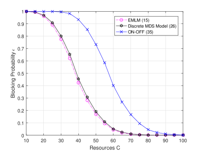
Figure 1: Blocking Probability Curve

Specifically, we choose $N=10000,\lambda=0.001,\mu=0.5,t_{s}=0.0001$ and $\sigma=0.5$. The requirement $X$ obeys the distribution

$$X\sim\begin{pmatrix}1&2&4&8\\ 0.45&0.35&0.15&0.5\end{pmatrix}.$$ (40)

Apparently, our discrete MDS Model (26) is close to EMLM (15), which implies the accuracy of our analysis. Under same parameter, community under ON-OFF model needs more resources to support compared with common situation.

V Conclusion

In this paper, the probabilistic models for the MDS are established. For general case , we analyzes blocking probabilities of MDS in three states: non-tolerance, tolerance and delay, as shown in (6), (7) and (10). When the requirements are co-distributed with respect to time, a mathematical proof shows that EMLM and ON-OFF model are applicable to MDS, as stated in Theorem III.1 and Theorem III.2. An method to pre-allocate resources for communication society is given in Algorithm 1 and Figure 1 of a toy example implies the correction of our theoretical deductions.

References

• [1] J.Β S. Vardakas, I.Β D. Moscholios, M.Β D. Logothetis, and V.Β G. Stylianakis. β€œPerformance analysis of ocdma pons supporting multi-rate bursty traffic,” IEEE Transactions on Communications, vol. 61, no. 8, pp. 3374–3384, 2013.
• [2] M.Β F. Ramalhoto. Erlang’s Formulas, Springer, Berlin, Heidelberg, pp. 451–455, 2011.
• [3] L.Β Gimpelson. β€œAnalysis of mixtures of wide- and narrow-band traffic,” IEEE Transactions on Communication Technology, vol. 13, no. 3, pp. 258–266, 1965.
• [4] M. D. Logothetis and I. D. Moscholios. β€œTeletraffic models beyond erlang,” In 2014 ELEKTRO, pp. 10–15, 2014.
• [5] I. D. Moscholios, J. S. Vardakas, M. D. Logothetis, and A. C. Boucouvalas. β€œCongestion probabilities in a batched poisson multirate loss model supporting elastic and adaptive traffic,” Ann. Telecommun, vol. 68, pp. 327 – 344, 2012.
• [6] I. D. Moscholios, M. D. Logothetis, A. C. Boucouvalas, and V. G. Vassilakis. β€œAn erlang multirate loss model supporting elastic traffic under the threshold policy,” In 2015 IEEE International Conference on Communications (ICC), pp. 6092–6097, 2015.
• [7] V.Β G. Vassilakis, G.Β A. Kallos, I.Β D. Moscholios, and M.Β D. Logothetis. β€œCall-level analysis of w-cdma networks supporting elastic services of finite population,” In 2008 IEEE International Conference on Communications (ICC), pp. 285–290, 2008.
• [8] J.Β Vardakas, I.Β Moscholios, M.Β Logothetis, and V.Β Stylianakis. β€œAn analytical approach for dynamic wavelength allocation in wdm–tdma pons servicing on–off traffic,” Journal of Optical Communications and Networking, vol. 3, no. 4, pp. 347–358, 2011.
• [9] N. Zychlinski, C. Chan, and J. Dong. β€œManaging queues with different resource requirements,” Operations Research, vol. 71, no. 4, pp. 1387-1413, 2020.
• [10] R. Durrett. Probability Theory and Examples, Cambridge University Press, Cambridge, 2019.
• [11] M. M-A. Asrin. β€œCall-burst blocking and call admission control in a broadband network with bursty sources,” Perform. Evaluation, vol. 38, pp. 1–19, 1999.
• [12] G. M. Stamatelos and V. N. Koukoulidis. β€œReservation-based bandwidth allocation in a radio atm lan,” In 1996 IEEE International Conference on Communications (ICC), pp. 1247–1253, 1996.