Novel operational algorithms for ride-pooling as on-demand feeder services

Abstract

Ride-pooling (RP) service, as a form of shared mobility, enables multiple riders with similar itineraries to share the same vehicle and split the fee. This makes RP a promising on-demand feeder service for patrons with a common trip end in urban transportation. We propose the RP as Feeder (RPaF) services with tailored operational algorithms. Specifically, we have developed (i) a batch-based matching algorithm that pools a batch of requests within an optimized buffer distance to each RP vehicle; (ii) a dispatching algorithm that adaptively dispatches vehicles to pick up the matched requests for certain occupancy target; and (iii) a repositioning algorithm that relocates vehicles to unmatched requests based on their level of urgency. We also embed the Traveling-Salesman-Problem (TSP) model to generate routing plans for each dispatched vehicle. An agent-based microscopic simulation platform is designed to execute these operational algorithms (via the Operator module), generate spatially distributed random requests (Patron module), and account for traffic conditions (Vehicle module) in street networks. Extensive numerical experiments are conducted to showcase the effectiveness of RPaF services across various demand scenarios in typical morning rush hours. We compare RFaF with two on-demand feeder counterparts proposed in previous studies: Ride-Sharing as Feeder (RSaF) and Flexible-Route Feeder-Bus Transit (Flex-FBT). Comparisons reveal that given the same fleet size, RPaF generally outperforms RSaF in higher service rates (i.e., the percentage of requests served over all requests) and Flex-FBT in shorter average trip times for patrons. Lastly, we illustrate the implementation of RPaF in a real-world case study of the uptown Manhattan network (USA) using actual taxi trip data. The results demonstrate that RPaF effectively balances the level of service (service rate and patrons’ average trip time) with operational costs (fleet size). The proposed simulation platform offers a valuable testbed for evaluating and optimizing various on-demand feeder services.

1 Introduction

The rise in ride-hailing mobility has posed significant challenges to traditional urban public transportation systems, causing a global decline in ridership since the 1990s (Graehler et al., 2019; Olayode et al., 2023). The onset of the COVID-19 pandemic has exacerbated this trend, prompting a further shift from public transportation to individual mobility (Luo et al., 2022; Shaheen and Wong, 2022). Evidence shows that transit ridership in most cities worldwide has yet to recover to pre-pandemic levels (Ziedan et al., 2023). This global phenomenon threatens the financial viability of many transit agencies, placing an increased burden on government subsidies.

To reverse this downward trend, some transit agencies are exploring innovative solutions to incorporate ride-hailing technologies into On-Demand Transit (ODT) services in hopes of luring back riders (Ghimire et al., 2024). One of the major applications of these technology-enabled ODTs is to connect transportation hubs and their service zone(s) where demand is too scattered and low to support the operation of fixed bus lines (Koffman, 2004). While ODT, sometimes referred to as demand-responsive transit or paratransit, is not a novel concept (Vuchic, 2007), the integration of ride-hailing technologies – such as smartphone-based wireless communication and global position systems (GPS) – elevates the user experience through dynamic responses, location-based services, seamless payment, and transparent information.

On the other hand, Transportation Network Companies (TNCs), as the platform provider of ride-hailing mobility, are introducing Ride-Pooling (RP) services as a first/last-mile solution to public transportation, either in partnership with transit agencies or independently (Shaheen and Cohen, 2019). RP services, such as Uber (Express) Pool, Lyft Line/Shuttle, Via Vanpooling, and Didi Express Pool, match multiple requests with similar itineraries to share the ride in the same vehicle. The RP not only improves transit accessibility as a faster feeder mode but also addresses the drawbacks of the conventional non-shared ride-hailing vehicles, which have been criticized for inducing individual trips, worsening traffic congestion, and increasing air pollution (Alonso-Mora et al., 2017; Furuhata et al., 2013; Chan and Shaheen, 2012).

Both the technology-enabled ODTs and RP are On-Demand Shared-Ride (ODSR) mobility that offers customized door-to-door routing services. However, they differ in several operational aspects, as noted by Fan et al. (2024a):

• ODTs generally adhere to schedule/frequency-based operation strategies, either fixed for reserved requests or flexible for dynamic requests (Shahin et al., 2024). Accordingly, ODTs dispatch vehicles sequentially at headways and match requests within each headway interval to successive vehicles. In such a “sequenced operation”, each ODT vehicle has to traverse the entire service zone where the matched requests are dispersed.

• In contrast, RP vehicles are distributed over the network and are matched with the closest requests, with dispatches triggered by successful matches. As a result, this “distributed operation” confines each RP vehicle’s pickup process within the neighborhood area of its current location.

Therefore, we see RP’s potential to lower pickup costs for operators and patrons. This motivates us to investigate: (i) whether RP could surpass ODTs in overall system performance; (ii) under what conditions this might occur; and (iii) to what extent the advantage would manifest. To address these questions, we focus on the “feeder problem” (also called first-mile and last-mile problem) framework (e.g., Clarens and Hurdle, 1975; Chang and Schonfeld, 1991b), where feeder services are operated to transport patrons with dispersed locations to/from a common hub. The feeder-problem scenario applies to various contexts, where the hub can be a subway station, a school, a shopping mall, a stadium, a convention center, etc., and the travel demand is derived from commuters, students, shoppers, and audiences. Several pioneering works have been done on designing ODTs in the feeder-problem framework (e.g., Chen and Nie, 2017a; Luo and Nie, 2019; Sangveraphunsiri et al., 2022). For comparison, we propose innovative operational algorithms for RP-as-feeder (RPaF) services.

The main contributions of this paper are threefold:

1. Three operational algorithms are tailored for RPaF services. They are (1) a batch-based matching algorithm that functions based on the buffer distance concept, ensuring that each RPaF vehicle is assigned requests within its neighborhood; (2) a dispatching algorithm that employs hard- and soft-target models to deploy vehicles according to fixed and variable occupancy targets, respectively; and (3) a repositioning algorithm that relocates vehicles to unmatched requests based on their level of urgency, which is quantified as a weighted sum of the time elapsed since the request was made and the distance between the request and the vehicle.

2. A microscopic simulation environment is developed to implement the proposed system as well as its ODSR counterparts. The simulation framework consists of three modules designed to capture the interactions among the operator, patrons, and vehicles. Such a module-based simulation framework serves as a testbed for evaluating the efficacy of the operational algorithms under diverse demand patterns in both stylized and real-world street networks.

3. Systematic comparisons are conducted between the proposed RPaF and two counterparts, namely Ride-Sharing as Feeder (RSaF) (Daganzo and Ouyang, 2019a; Liu and Ouyang, 2021) and Flexible-Route Feeder-Bus Transit (Flex-FBT) (Chen and Schonfeld, 2022; Liu and Schonfeld, 2020; Kim et al., 2019; Kim and Schonfeld, 2013, 2012; Chang and Schonfeld, 1991b), which have been previously studied as on-demand feeder services. Their operational details are provided in Section 5.3. Our study elucidates the impacts of their operational differences and delineates the application domains of RPaF through extensive experiments. Furthermore, a real-world case study contrasts the three ODSR modes with the current non-shared taxis.

The remainder of this paper is organized as follows. The next section reviews related studies. Then, Section 3 develops key operational algorithms for RPaF, which are embodied into the module-based simulation platform in Section 4. Section 5 presents numerical studies that examine the operational algorithms and compare alternative on-demand feeder systems. A real case study is demonstrated in Section 6 using taxi trip data in uptown Manhattan, New York, USA. Finally, Section 7 concludes this paper. Since there are several abbreviations, Table 1 in A lists them along with their meanings for the reader’s convenience.

2 Related studies

Feeder services are essential in transit networks to enhance accessibility, facilitating passengers to travel between transit stations and their various origins and destinations. Research on feeder services is extensive and can be categorized by transportation modes (Malucelli et al., 1999; Errico et al., 2013). Traditional feeder modes comprise (i) on-demand individual modes, e.g., walking, cycling (private or shared) bikes, driving (private or shared) cars, and non-shared ride-hailing taxis, and (ii) fixed shared-ride modes, e.g., Fixed Feeder-Bus Transit (Fix-FBT). However, these modes often exhibit notably poor performance in one or more of the three transportation aspects: mobility, accessibility, and efficiency, as summarized in Table 1.

Table 1: Qualitative comparisons between RPaF and other feeder modes

Feeder mode	Characteristics
Ride-Pooling as Feeder (RPaF)	On-demand shared-ride door-to-door service; distributed operation*; vehicle occupancy of 2$\sim$7; private/dedicated drivers or autonomous driving; average in-vehicle speed of 15$\sim$50 km/h
Alternatives1	Characteristics	Versus RPaF
Walking	On-demand individual mobility; average speed of 2$\sim$5 km/h	Low speed (mobility)
Cycling (private or shared) bikes	On-demand individual mobility; borrow and return shared bikes anytime, anywhere; average riding speed of 5$\sim$12 km/h	Riding eligibility required; low speed (mobility)
Driving (private or shared) cars	On-demand individual mobility; one-way or two-way mobility; average riding speed of 15$\sim$60 km/h	Driving eligibility required; low vehicle occupancy (efficiency)
Non-shared ride-hailing taxis	On-demand individual door-to-door service; distributed operation (matching; dispatching); dedicated drivers; average operation speed 15$\sim$60 km/h	Low vehicle occupancy (efficiency)
Fixed feeder-bus	Traditional shared-ride stop-to-stop services; fixed routes, stops, schedules; vehicle occupancy of 2$\sim$25; average in-vehicle speed of 15$\sim$40 km/h	Low accessibility
On-Demand Transit (ODT)	On-demand shared-ride door-to-door service; flexible route/stop for door-to-door services; sequenced operation**; vehicle occupancy of 2$\sim$15; dedicated drivers or autonomous driving; average in-vehicle speed of 15$\sim$40 km/h	To be studied in this paper

• The literature on RP and ODT are discussed in detail as follows. For those of shared bikes, see Luo et al. (2021); Wu et al. (2020); Li et al. (2023). See Aldaihani et al. (2004); Chen and Nie (2017a, b); Ramezani and Valadkhani (2023) for non-shared taxis. See Jorge et al. (2015) for carsharing. And Sivakumaran et al. (2014) for fixed feeder-bus transit.

• Distributed operation means that matching vehicles and requests based on their proximity in the network and successful matches determine the dispatches of the vehicles.

• Sequenced operation means dispatching vehicles by headways and matching requests during the time interval to successive vehicles.

Combining on-demand and shared-ride properties, ODT and RP aim to balance the above three inherently conflicting aspects. Particularly, RP/ODT-as-feeder services demonstrate potential by streamlining the matching and transportation of multiple requests with a common trip end, making them more efficient compared to serving many-to-many (M2M) demands (Errico et al., 2021). The state-of-the-art research of the two innovative feeder modes is summarized as follows. For general RP and ODT with M2M demands, interested readers can refer to recent surveys such as Mourad et al. (2019) and Vansteenwegen et al. (2022).

We begin with the early development of ODSR systems that served as the precursor to modern ODT and RP.

2.1 Early on-demand shared-ride feeder services

The early ODSR system primarily consisted of Dial-A-Ride (DAR) services, which operated on a reservation basis depending on 20th-century communication technologies such as the telephone and the Internet. These services are commonly used by captive passengers with low travel frequency, including individuals with disabilities who require transportation to hospitals or workplaces.

DAR-as-feeder studies date back to Wilson et al. (1976), Wilson and Roos (1968), and Wilson and Hendrickson (1980), and then developed by many scholars such as Liaw et al. (1996), Hickman and Blume (2001), and Aldaihani and Dessouky (2003). Due to its reservation-based low-frequency operational characteristics, DAR-as-feeder research primarily focuses on routing and scheduling problems for one-time out-of-depot vehicle trips. In this setting, each vehicle in the fleet is tasked with a single depot-based round trip for picking up or dropping off its assigned passengers within its capacity constraint. Constraints from the passengers’ side are also respected such as their preferred time windows and maximum ride duration. The goal is usually to minimize the total vehicle distance traveled. These tactical operational problems are called static DAR Problems (DARP) with one-to-many (O2M) and many-to-one (M2O) demand. Variant models have been developed in the DARP framework, such as those employing different routing policies (Feng et al., 2014), considering irregular street networks (Pan et al., 2015), allowing meet points for multiple passengers boarding and alighting (Li et al., 2018), and using alternative mathematical approaches (Yu et al., 2015). Both exact and heuristic solution algorithms are developed for the proposed problems; see Cordeau and Laporte (2003) for an overview.

Dynamic DARPs have also been developed to tackle en-route instantaneous pickup requests or cancellations. The main trade-off is between the benefits/costs of the reserved passengers and last-minute requests. A common objective is to maximize the number of served passengers. Various approaches are proposed to facilitate the insertion of future requests into the existing schedule and routing plan. For instance, Wang et al. (2020) modeled a two-step dynamic DARP, in which the first step constructs the initial routing and scheduling plan, and the second step modifies it to respond to real-time requests. A thorough survey can be found in Ho et al. (2018).

The static and dynamic DARP studies enhance fundamental theories for vehicle routing and scheduling of ODSR services. Yet, increasing demand driven by advanced communication technologies poses new operational challenges, necessitating ODSR vehicles to operate dynamically for multiple round trips between the hub and service areas. The management of recurrent vehicle trips determines whether ODSR evolves into ODT and RP under sequenced or distributed operations, respectively.

2.2 ODT-as-feeder services

ODT-as-feeder services can be further divided into two groups: (i) flexible and (ii) semi-flexible feeder-bus transit, with the latter adhering partially to fixed routes/stops and timetables, permitting spontaneous deviations.

(i) Flexible Feeder-Bus Transit (Flex-FBT): Flex-FBT studies emerge in the 1970s with Clarens and Hurdle (1975) and Ward (1975). To confine the vehicle distance traveled for serving dispersed demand, zoning strategies have been utilized to divide the service area into smaller zones, each with dedicated buses. Flex-FBT research focuses on macroscopic system designs, rather than specific routing and scheduling plans, involving determinations of zone areas, headways, fleet sizes, and bus capacities. Analytical models have been developed to estimate system costs for operators and passengers. These models rely on approximations of average vehicle tour lengths for multiple pickups and drop-offs (Stein, 1978; Daganzo, 1978, 1984).

The system-design modeling framework is adopted by subsequent studies. For instance, Wirasinghe et al. (1977) jointly optimized a rail line and its Flex-FBT. Jacobson (1980) compared the Flex-FBT system with direct door-to-door services and unveiled the crucial impact of transfer penalties on the performance of Flex-FBT. Adebisi and Hurdle (1982) presented a comparative analysis for choosing between a Flex-FBT and a single fixed bus line according to the ridership levels. Chang and Schonfeld (1991a, b) further compared Flex-FBT and Fix-FBT and accordingly proposed integrating the two options for lower- and higher-demand periods, respectively.

The comparison between Flex- and Fix-FBT remains an attractive topic in subsequent studies such as Edwards and Watkins (2013) using real-world survey data, Badia and Jenelius (2021) using automated buses, and Leffler et al. (2021) in different network structures. The analytical models obtained by Chang and Schonfeld (1991a, b) were then extended by several studies for varying contexts, such as mixed fleets (e.g., Kim and Schonfeld, 2012, 2013), coordinated schedules (e.g., Kim and Schonfeld, 2014), joint optimization of the service area and headway (e.g., Kim et al., 2019; Chen et al., 2020) and auto buses (e.g., Guo et al., 2017; Liu and Schonfeld, 2020). Huang et al. (2019) further employed the modeling framework to consider travelers’ departure time choices.

(ii) Semi-flexible Feeder-Bus Transit (Semiflex-FBT): Semiflex-FBT, also called Mobility Allowance Shuttle Transit (MAST) or Demand Adaptive Transit (DAT), generally operates in a corridor following pre-specified routing policies. Welch et al. (1991) is among the earliest works to introduce the concept of Semiflex-FBT, highlighting the trade-off between increased accessibility of on-demand detours and the negative impact on the mobility of through riders. Fu (2002) developed an analytical theory for Semiflex-FBT system designs regarding the optimal slack time between consecutive fixed stops to absorb random detours. A similar work is Crainic et al. (2012), who turned to design specific time windows at the fixed stops. Smith et al. (2003) further included the service zone size of Semiflex-FBT as the key design variable.

The work of Quadrifoglio et al. (2006) has a significant impact on subsequent research. The author conducted an analytical analysis to approximate the Semiflex-FBT vehicle tour length under a specific routing strategy, known as the no-backtracking policy (Daganzo, 2005). The closed-form models obtained by Quadrifoglio et al. (2006) laid the foundation for the optimal system design of Semiflex-FBT in several works (e.g., Zhao and Dessouky, 2008; Quadrifoglio and Li, 2009; Li and Quadrifoglio, 2011; Chandra and Quadrifoglio, 2013; Papanikolaou and Basbas, 2021; Sangveraphunsiri et al., 2022). Alternative routing strategies have been explored, such as combinations of Fix/Flex-FBT, shortcuts, and short turns (Ceder, 2013), dynamic station strategy (Qiu et al., 2014, 2015a, 2015b, 2015c), route and point deviation strategies (Zheng et al., 2018), meeting point strategy (Zheng et al., 2019), and fixed route with flexible stopping schedule (Mehran et al., 2020).

It is worth noting that Nourbakhsh and Ouyang (2012) expanded Semiflex-FBT to a structured transit network for monocentric cities. Analytical models were developed for optimizing system designs concerning the service zone size and headway of each Semiflex-FBT line as well as a network structure parameter (i.e., the central zone area). Chen and Nie (2017a, 2018) further integrated Semiflex-FBT with the fixed-route transit network and jointly optimized the integrated system in grid and radial street network structures. Calabrò et al. (2023) advanced the integrated system design by relaxing the assumption of spatially uniform demand distribution in Nourbakhsh and Ouyang (2012) and Chen and Nie (2017a, 2018). In such integrated systems, Leffler et al. (2024) introduced mode- and route-choice models for passengers to capture the day-to-day learning process and the demand splits among multiple transit modes.

In contrast to the above system design studies, attention was also paid to the vehicle routing problem of Semiflex-FBT as a variant of DARPs with partial fixed stops. Crainic et al. (2005) tested several meta-heuristic solution algorithms (including the tabu search method and greedy multitrial randomized method) to solve the routing problem of a single-line Semiflex-FBT, which was later attacked using customized heuristic algorithms (Errico et al., 2021). Other meta-heuristic algorithms have also been investigated, such as a multi-stage solution algorithm based on space partitioning and the genetic algorithm (Lu et al., 2016), and a large neighborhood search algorithm (Montenegro et al., 2021). A comprehensive survey is available in Shahin et al. (2024).

2.3 RP-as-feeder services

Technology-enabled RP contrasts with previous ODSR services primarily in its dynamic operational characteristics (Shen et al., 2018). The ordering, matching, and dispatching of RP vehicles are executed in a distributed manner, without a specific sequence, and are completed in minutes or seconds. This dynamic and distributed context gives rise to new research topics, including the vehicle-request matching problem (Santi et al., 2014; Yang et al., 2020; Ramezani and Valadkhani, 2023), the idling vehicle rebalancing problem (Alonso-Mora et al., 2017; Simonetto et al., 2019; Valadkhani and Ramezani, 2023), and fare splitting problem (Ke et al., 2020; Zhang and Nie, 2021), besides the classic vehicle routing problem (formulated as dynamic DARPs) (Ho et al., 2018; Namdarpour et al., 2024).

RPaF is a variant of general-purpose RP for M2M demand (Agatz et al., 2012; Furuhata et al., 2013). RPaF can be further divided into three groups according to who drives the vehicles: (i) shared taxis with dedicated drivers hired by taxi companies or transit agencies, (ii) Peer-to-Peer (P2P) ride-sourcing/sharing, where private car owners participate in the crowd-sourced mobility platforms such as those of TNCs, and (iii) Autonomous Vehicles (AVs) that operate without human drivers.

(i) Shared Taxi-as-Feeder (STaF): Tao (2007) is among the first to apply the shared-taxi concept (previously developed in Frattasi et al., 2005) to airport access. The STaF services are then evaluated by Tao and Wu (2008) and Ma et al. (2017) using empirical data. Ma et al. (2019) considered STaF at both access and egress ends of transit trips and simulated for a case study of Long Island rail transit commuters to New York City. Bian and Liu (2019a, b) conducted mechanism designs (including vehicle-request matching, vehicle routing, and pricing strategies) for STaF accounting for personalized requirements, such as extra in-vehicle travel time, the number of co-riders, and early-arrival waiting time at the transit hub. Zhu et al. (2020b) modeled shared taxis as both a feeder and an alternative to transit. They found the STaF-transit structure can benefit all three parties, i.e., the taxi operator, transit agency, and passengers. Liu and Ouyang (2021) employed an overarching analytical framework for the joint design of STaF and transit systems. The design variables include the fleet size and zoning of STaF as well as the line spacing and headway of the transit network. They found that the integrated system can outperform the conventional transit systems fed by walking, Fix-FBT, and non-shared taxis.

(ii) P2P Ride-Sharing-as-Feeder (RSaF): The vehicle routing problems of P2P-RSaF are a novel variant of DARP, which involves private drivers’ heterogeneous travel preferences and were initially studied by Masoud and Jayakrishnan (2017); Stiglic et al. (2018). Kumar and Khani (2021) suggested integrating P2P-RSaF with a schedule-based transit system. A rolling horizon approach was applied to solve dynamic ride-sharing with transfers at transit stops. Nam et al. (2018) resorted to simulation tools to examine the effects of P2P-RSaF on the Los Angeles Metro Red Line subway rail. However, P2P-RSaF may not be a viable feeder mode for the general public because private drivers may impose stringent constraints and not comply with scheduling requirements. These issues can be addressed by leveraging AVs.

(iii) Shared AVs-as-Feeder (SAVaF): Driven by advancements in AV technology, the role of SAVaF in transit systems has been recognized (Shen et al., 2018; Wen et al., 2018). For instance, Shen et al. (2018) simulated SAVaF to replace low-demand Fix-FBT routes for the subway in Singapore. Wen et al. (2018) simulated SAVaF among other feeder modes to rail stations. Chen et al. (2020) studied SAVaF to a single subway station and formulated a static DARP for each epoch in a rolling horizon framework. Gurumurthy et al. (2020) and Huang et al. (2021a) simulated and compared integrated transit systems fed by SAVaF and direct door-to-door services in Austin (Texas, USA). Pinto et al. (2020) simulated a transit network with SAVaF and jointly optimized the transit service frequency and the fleet size of AVs. Imhof et al. (2020) evaluated the feasibility of SAVaF connecting railway stations in the rural area of the Toss Valley, Switzerland. Lau and Susilawati (2021) estimated the transit demand brought by SAVaF considering travelers’ mode choice preferences in Kuala Lumpur (Malaysia). Whitmore et al. (2022) examined the cost efficiency of integrating SAVaF for equitable transit coverage in Allegheny County, Pennsylvania (USA).

2.4 Research gap

We now summarize the above literature review and then identify research gaps to be addressed in this paper.

Four key points can be drawn from the literature review:

• Early research on ODSR services surrounds the development of DARP theories, resulting in fruitful outcomes such as variant context-specific DARP models, exact solution algorithms, and (meta-)heuristic solution algorithms. These achievements have established the groundwork for vehicle routing and scheduling for both ODT- and RP-as-feeder services.

• The advance in ride-hailing technologies induced dynamic demand and transformed ODSR into ODT- and RP-as-feeder, which inherit operational features from traditional transit and taxi services, respectively. The former adopts zoning strategies and employs cyclical headway-based operation for each zone, while the latter intercepts trip requests based on temporal-spatial proximity to distributed vehicles in the network.

• Research on ODT-as-feeder has focused on system designs using approximation-based analytical models. System performance evaluations have demonstrated that ODT-as-feeder services can offer substantial advantages over traditional feeder modes (e.g., walking, non-shared taxis, and Fix-FBT) for low-density demand situations.

• Much effort of RP-as-feeder research has been devoted to addressing the new operational challenges, such as dynamic vehicle-request matching and vehicle rebalancing among others. Existing studies on the performance evaluation of RP-as-feeder services mostly involve early-stage concept designs, scenario simulations, and analytical analyses for optimal system designs. RP-as-feeder also proves beneficial in low-density demand scenarios.

As seen, both ODT- and RP-as-feeder exhibit advantages over traditional feeder modes in low-density demand scenarios. It is natural to question which of the two performs better and the application ranges distinguishing them. However, the existing literature lacks systematic comparisons between the two feeder modes, overlooking the impact of their subtly distinct operational features. An exception is Fan et al. (2024a), which compared a novel RP variant, RP with the Hold-Dispatch strategy (RP-HD), and Flex-FBT. Analytical models were developed for optimizing system designs under non-uniform demand distributions. Extensive numerical experiments demonstrated that RP-as-feeder services consistently outperform Flex-FBT in all test scenarios except when the fleet cost/patrons’ value of time becomes much higher/lower.

Nevertheless, Fan et al. (2024a) is a macro-level study based on aspatial queueing models that overlooked network structures and operational details like vehicle-request matching, vehicle dispatching, routing, and repositioning. This study will address these aspects in specific street networks and devise sophisticated operational algorithms that were previously ignored in the cited study for tractability. Building on the research by Fan et al. (2024a), we aim to delve deeper into the efficacy of RPaF in stochastic and dynamic circumstances. To achieve this, we employ a simulation-based approach. Simulation models serve as ideal tools to execute theoretical service designs in realistic situations accounting for the impacts of many random factors. Laboratory experiments can be easily conducted across various scenarios to offer guidance for real-world applications.

Numerous simulation-based tools have been developed for the operation of ODSR-as-feeder systems, such as customized micro-simulation platforms for DAR (Wilson and Hendrickson, 1980), Flex-FBT (Ceder, 2013; Edwards and Watkins, 2013; Leffler et al., 2021), Semiflex-FBT (Horn, 2002a, b; Yoon et al., 2022; Leffler et al., 2024), STaF (Ma et al., 2019), P2P-RSaF (Masoud and Jayakrishnan, 2017; Kumar and Khani, 2021), and SAVaF (Wen et al., 2018; Pinto et al., 2020), along with open-source multi-agent simulation software like MATSim (Gurumurthy et al., 2020) and SUMO (Huang et al., 2021a) for SAVaF. This paper adds a new tool to the arsenal for simulating RPaF services with innovative operational algorithms described below.

3 RPaF with novel operational algorithms

We begin with the RPaF service description in Section 3.1, followed by novel operational algorithms in Section 3.2. In line with existing on-demand feeder systems (e.g., RSaF and Flex-FBT), we focus on dynamic, and spontaneous (rather than reservation-based) trips, where patrons typically indicate only their desired pick-up and/or drop-off locations. The notations used in this paper are summarized in Table 2 of A.

3.1 RPaF service description

We adopt the RPaF concept from (Fan et al., 2024a), which connects a remote suburb and a downtown hub, as illustrated in Figure 1. Similar layouts have been used in previous studies to study feeder transit systems, e.g., Kim et al. (2019); Kim and Schonfeld (2013). We use this single-hub system to ensure comparability with prior research. In cases of networks with multiple hubs, the proposed models can be utilized to operate separate RPaF services for each hub.

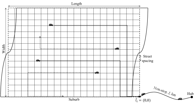
Figure 1: Illustration of ride-pooling as on-demand feeder services.

As shown in Figure 1, we first represent the suburb as a rectangular suburban region with an evenly spaced grid street network. (Later, we will apply the simulation framework to a case study using the real-world street network and demand data.) We aim to examine a stabilized system, where the roadway network is configured with the following traffic characteristics. The cruising speed of RPaF vehicles is $S^{\prime}$ [km/h] on suburban streets and $S$ [km/h] on freeways. At intersections, RPaF vehicles experience delays dependent on control rules such as no control and signalized controls. In addition, vehicles incur a fixed delay $t_{d}$ [seconds] for each stop to pick up or drop off. To enhance simulation efficiency, we disregard the dynamics of background traffic, which may have a minor impact in suburban areas. The simulation of dynamic traffic could be integrated into our framework as a potential future research direction.

The travel demand between the suburb and the hub is bidirectional, denoted $\lambda_{\rm OB}$ [patrons/sq. km/hour] for outbound trips (from residences in the suburb to the hub) and $\lambda_{\rm IB}$ [patrons/sq. km/hour] inbound trips (from the hub to the suburb). We assume for now that travelers’ origins and destinations are uniformly distributed throughout the suburban area. This assumption will later be lifted in the real case study. Following previous studies (e.g., Daganzo and Ouyang, 2019a; Kim et al., 2019; Liu and Ouyang, 2021), we also assume that the demand is known and inelastic to RPaF service changes. (Induced demand can also be integrated into the simulation framework, but this is left for future study.)

We will examine a single RPaF operator who oversees a fleet of e-hailing vehicles with fully compliant drivers. This operator could be a TNC, a transit agency, or a third-party integrator that combines services from various providers onto a unified platform. This setup reduces fierce competition among different operators and allows for pooling multiple requests without the concern of losing them to other competitors. Therefore, we suppose travelers do not cancel their orders within a maximum tolerance time $\bar{\tau}$ or after the vehicles are dispatched.

3.2 Operational algorithms

This section develops four key operational algorithms for the above RPaF service, i.e., the matching, dispatching, routing, and repositioning algorithms.

3.2.1 Matching algorithm

The matching algorithm is deployed to match the spatially distributed (outbound) vehicles and patrons. Note that inbound vehicles and patrons meet at the hub’s pick-up area and thus do not need online matching. Therefore, the subsequent discussion of the matching algorithm refers to outbound service.

Following (Ma et al., 2017; Yang et al., 2020; Wei et al., 2022), we adapt the “batch-based matching” algorithm by using a target number of requests $U$ instead of a pre-specified time window, which will be explained soon. This algorithm pools $U$ requests into batches for each available vehicle within its matching buffer distance of $\Delta$ [km]. The algorithm then assigns the vehicles with the $u$ closest requests out of $U$. The unmatched requests ($U-u$) in the last batch are prioritized over new incoming requests in the following matching round. The steps of the batch-matching algorithm are outlined in Algorithm 1. The matching algorithm outputs a vehicle-request mapping dictionary $\mathbf{X}=\{X_{n}\}$.

The proposed algorithm differs from most existing ones, which depend on integer programming with bipartite graphs (see, e.g., Ramezani and Valadkhani, 2023). The distinction, however, enables our algorithm to yield the following valuable analytical properties absent in mathematical programming models and consequently reduces the computational complexity significantly.

Algorithm 1 Batch-based matching algorithm

Input: At the current simulation time $t$, request set $R\equiv\left\{r_{i}=\langle t_{i},\vec{l}_{i},\delta_{i}\rangle\right\}$, vehicle set $V\equiv\left\{v_{n}=\langle o_{n},\vec{l}_{n},X_{n},\delta_{n}\rangle\right\}$, matching buffer distance $\Delta$;
  Output: At the current simulation time $t$, vehicle-demand mapping dictionary $\mathbf{X}\equiv\{X_{n}\}$.

1:Attain the last simulation time $\mathbf{X}=\{X_{n}\}$.

2:for each vehicle $n$ in $V$ do

3:     if vehicle state $v_{n}=\langle 0,\vec{l}_{n},X_{n},\text{OB}\rangle$ and $|X_{n}|<u$ state then

4:         Let vehicle $n$ be the candidate vehicle.

5:         Calculate the remaining vehicle capacity $u-|X_{n}|$.      

6:     Define set $\mathbf{D}_{n}=\{d_{n,i}\}$ where $\{d_{n,i}\}$ denotes the distance between the

7:candidate vehicle $n$ and the candidate patron $i$ in $R$.

8:     for each patron $i$ in $R$ do

9:         if patron state $r_{i}=\langle t_{i},\vec{l}_{i},0\rangle$ then

10:              Calculate distance $d_{n,i}$ between vehicle $n$ and patron $i$.                    $\left.\rule{0.0pt}{28.79993pt}\right\}\ \mbox{in parallel}$ 11:              if $d_{n,i}\leq\Delta$ then $\left.\rule{0.0pt}{110.39996pt}\right\}\ \mbox{in parallel}$ 12:                  $\mathbf{D}_{n}\leftarrow\mathbf{D}_{n}\cup\{d_{n,i}\}$.                              13:     $m=\text{min}\left(u-|X_{n}|,|\mathbf{D}_{n}|\right)$. 14:     $\mathbf{D}_{n}^{*}={\rm sort}(\mathbf{D}_{n}=\{d_{n,i}\})$ in increasing distance order. 15:     Filter the first $m$ elements($\{d_{n,i}^{*}\}$) from the $\mathbf{D}_{n}^{*}$. 16:     $X_{n}\leftarrow X_{n}\cup\{i\}$, where $\{i\}$ corresponds to $\{d_{n,i}^{*}\}$. 17:     $r_{i}=\langle t_{i},\vec{l}_{i},1\rangle$, where $\{i\}$ corresponds to $\{d_{n,i}^{*}\}$. 18:     $v_{n}\leftarrow v_{n}=\langle 0,\vec{l}_{n},X_{n},\text{OB}\rangle$. 19:return $\mathbf{X}=\{X_{n}\}$.

The choice of parameters $U$ and $\Delta$ is crucial for the algorithm. We propose the following recipe to determine proper values that minimize patrons’ time delays in matching and subsequent routing processes. First, we notice that the matching buffer distance $\Delta$ defines a coverage area of $A(\Delta)$ [km²] for each available vehicle, e.g., $A(\Delta)=2\Delta^{2}$ in the Manhattan metric or $A(\Delta)=\pi\Delta^{2}$ in the Euclidean metric. In this area, pooling $U$ requests takes an average time of

$$\frac{U-\left(U-u\right)}{\lambda_{\rm OB}A(\Delta)}=\frac{u}{\lambda_{\rm OB}A(\Delta)},$$ (1)

where $\left(U-u\right)$ is the number of requests left from the last batch and only $u$ new requests need to be pooled per batch.

For patrons in the current batch and those in the following, they experience respectively half and the entire pooling time for $U$ requests. Thus, their total pooling time delays can be estimated by

$$u\frac{u}{2\lambda_{\rm OB}A(\Delta)}+\left(U-u\right)\frac{u}{\lambda_{\rm OB}A(\Delta)}.$$ (2)

In addition, the average travel time for visiting $u$ points within an area of $A(\Delta)$ can be approximated by

$$\frac{k\sqrt{A(\Delta)u}}{S^{\prime}(u)}\frac{u}{U+1},$$ (3)

where the expected tour distance of traveling-salesman-problem (TSP) with $u$ visiting points, i.e., $k\sqrt{A(\Delta)u}$ according to Stein (1978), is reduced by a factor of $\frac{u}{U+1}$, capturing the effect of filtering $u$ closest-to-the-vehicle requests out of $U$, as illustrated in Figure 2. The $k$ is a constant parameter, e.g., $k=1.15$ in Manhattan metric and $k=0.90$ in in Euclidean metric. The $S^{\prime}(u)$ is the vehicles’ commercial speed and satisfies $\frac{1}{S^{\prime}(u)}=\left(\frac{1}{S^{\prime}}+ut_{d}\right)$ considering stopping delays $t_{d}$.

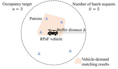
Figure 2: Illustration of “batch-based matching”(filtering $u$ closest-to-the-vehicle requests out of $U$).

Thus, patrons’ total TSP-tour delays, encompassing both out-of-vehicle and in-vehicle waiting times, can be estimated by

$$u\frac{k\sqrt{A(\Delta)u}}{S^{\prime}(u)}\frac{u}{U+1}+(U-u)\frac{k\sqrt{A(\Delta)u}}{S^{\prime}(u)}\frac{u}{U+1}=U\frac{k\sqrt{A(\Delta)u}}{S^{\prime}(u)}\frac{u}{U+1},$$ (4)

where the first term accounts for the first-matched $u$ patrons’ TSP-tour delays, and the second for the next-matched $(U-u)$ ones’, which occur in their respective and independent TSP tours. Note that the next matching occurs with another nearby vehicle and is independent of the completion of the first-matched vehicle’s pick-up task. We also note that the second term in Eq. (4), i.e., $(U-u)\frac{k\sqrt{A(\Delta)u}}{S^{\prime}(u)}\frac{u}{U+1}$, is an approximation. It assumes that the reduction effect of “filtering $u$ closest-to-the-vehicle requests out of $U$” is not compromised by the prioritized $(U-u)$ requests (which may not belong to the $u$ closest-to-the-vehicle requests) in the next matching pool. Nonetheless, this approximation term will cancel out when $U=u$, making Eq. (4) accurate, which will be met by the following optimization.

Adding Eqs. (2) and (4) yields total delays in the pooling and picking-up processes that are directly dependent on $U$ and $\Delta$:

$$U\frac{k\sqrt{A(\Delta)u}}{S^{\prime}(u)}\frac{u}{U+1}+u\frac{u}{2\lambda_{\rm OB}A(\Delta)}+\left(U-u\right)\frac{u}{\lambda_{\rm OB}A(\Delta)}.$$ (5)

We now determine $U$ and $\Delta$ by minimizing Eq. (5):

$$\operatorname*{minimize}_{U,A(\Delta)}U\frac{k\sqrt{A(\Delta)u}}{S^{\prime}(u)}\frac{u}{U+1}-\frac{u^{2}}{2\lambda_{\rm OB}A(\Delta)}+\frac{uU}{\lambda_{\rm OB}A(\Delta)}$$ (6a)

subject to:

$$U\geq u,A(\Delta)>0.$$ (6b)

Through a few steps derivation according to the first-order condition, problem (6) yields the following closed-form solutions:

$$U^{*}=u,A^{*}(\Delta)=u^{-\frac{1}{3}}\left[\frac{\left(u+1\right)S^{{}^{\prime}}(u)}{k\lambda_{\rm OB}}\right]^{\frac{2}{3}},$$ (7)

implying the optimal matching buffer distance to be

$${\Delta^{*}}=\begin{cases}&\left(8u\right)^{-\frac{1}{6}}\left[\frac{\left(u+1\right)S^{{}^{\prime}}(u)}{1.15\lambda_{\rm OB}}\right]^{\frac{1}{3}}\approx 0.675u^{-\frac{1}{6}}\left(\frac{\left(u+1\right)S^{\prime}(u)}{\lambda_{\rm OB}}\right)^{\frac{1}{3}},\text{ in Manhattan metric}\\ &\left(\pi^{3}u\right)^{-\frac{1}{6}}\left[\frac{\left(u+1\right)S^{{}^{\prime}}(u)}{0.9\lambda_{\rm OB}}\right]^{\frac{1}{3}}\approx 0.584u^{-\frac{1}{6}}\left(\frac{\left(u+1\right)S^{\prime}(u)}{\lambda_{\rm OB}}\right)^{\frac{1}{3}},\text{ in Euclidean metric}.\end{cases}$$ (8)

Remark: The above results indicate that the optimal batch size should be identical to the occupancy target $u$. In other words, no one should be left unmatched to the next batch. This result also explains why a time-window-based batch matching would probably be less effective, as $U\geq u$ would be generated in one or multiple pooling time windows until vehicles are dispatched upon at least $u$ matched requests. Another finding from Eq. (8) is that the optimal matching buffer distance $\Delta^{*}$ should increase/decrease as the demand density falls/rises with a power of $-\frac{1}{3}$. Eq. (8) also implies that larger $u$’s require longer matching buffer distances to shorten the pooling time, which outweighs the increase in TSP-tour time.

For those unmatched requests (with $\delta_{i}=0$), e.g., those out of the coverage areas of any vehicles, we sort them in the set $\widetilde{X}_{0}$ (of a virtual vehicle indexed by $0$) in an increasing order of their call-in times. They will be visited by the vehicles designated by the repositioning algorithm. It is noted that the relocated vehicles may encounter $U>u$ awaiting requests in their matching buffer distances upon their arrival (i.e., the beginning of matching). In this over-saturated case, the matching to the relocated vehicles will be performed based on requests’ “urgency”, which will be soon defined in the repositioning algorithm. The $\widetilde{X}_{0}$ is updated upon each match by removing $\{i|x_{n,i}=1,\forall n>0\}$.

3.2.2 Dispatching algorithm

This algorithm also functions for the outbound service since inbound vehicles follow the stop-and-go rule, as described in subsection 4.3. Following the idea of Fan et al. (2024a), we first incorporate a “hard-target” dispatch strategy that dispatches vehicles when the number of request assignments reaches the pre-given occupancy target, i.e., $|X_{n}|=u$. The steps are outlined in Algorithm 2.

Algorithm 2 Dispatching algorithm

Input: At the current simulation time $t$, vehicles set $V\equiv\left\{v_{n}=\langle o_{n},\vec{l}_{n},X_{n},\delta_{n}\rangle\right\}$, vehicle-demand mapping dictionary $\mathbf{X}\equiv\{X_{n}\}$.

1:Attain $V_{n}$ and $\mathbf{X}$.

2:for each vehicle $n$ in $V$ do

3:     Attain $X_{n}\in\mathbf{X}$.

4:     if $X_{n}=\emptyset$ state then

5:         The vehicle $n$ heads to the assigned location (under the instructions of

6:the repositioning algorithm in Algorithm 3).

7:     else if $|X_{n}|=1$ then

8:         if dispatch interval $t_{n}$ = None then

9:              Set $t_{n}=t+\bar{\tau}$ $\left.\rule{0.0pt}{76.79993pt}\right\}\ \mbox{in parallel}$          

10:     else if $1<|X_{n}|<u$ and departure interval $t_{n}$ is not reached then

11:         The vehicle $n$ remains stationary.

12:     else if $|X_{n}|=u$ or $t$ reach departure interval $t_{n}$ then

13:         The vehicle $n$ is dispatched to the first request point followed by the

14:routing algorithm.      

As found by Fan et al. (2024b), the hard-target dispatch strategy outperforms its counterparts, e.g., a “quick-dispatch” strategy in Daganzo and Ouyang (2019a) and a headway-based strategy (of which the details in given in C and D) under medium to high levels of demand.

Nonetheless, as noticed by Daganzo and Ouyang (2019b), the hard-target dispatch strategy may cause prolonged wait delays to the arrived requests due to the late arrivals of the last few requests for a full match of $u$ requests. To address this issue, we modify the hard target to be a “soft target”, with slightly abused notation $u(\tau)$, that decreases gradually as the time $\tau$ elapses since the vehicle’s first request assignment, as illustrated in Figure 3.

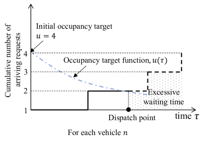
Figure 3: Illustration of soft-target dispatch strategy in RPaF.

Several forms of time-declining models have been proposed for $u(\tau)$, of which a simple one is as follows (Fan et al., 2024b):

$$u(\tau)=\min\left\{\frac{2c_{f}}{\beta\tau},u\right\},$$ (9)

where $u$ is the original fixed hard target; $c_{f}$ is the operational cost per dispatch; and $\beta$ denotes patrons’ value of time (VOT). The derivation of Eq. (9) can be found in Daganzo and Ouyang (2019b); Fan et al. (2024b) and thus, is omitted here. It is worth noting that Fan et al. (2024b) found that the soft-target strategy performs better for shuttle transit systems under demand distributions with large coefficients of variation, and the hard-target strategy is suitable for patrons with low VOTs (or equivalently when operational cost is high). This paper will examine two dispatching strategies for RPaF services.

In addition, we will modify the dispatching algorithms to include a maximum interval since the first request arrived in the matching pool. The modification aims to mitigate the request-canceling issue to prevent excessive cancellations that could harm customer satisfaction and reduce demand. This maximum dispatch interval is set equal to patrons’ maximum tolerance time $\bar{\tau}$.

3.2.3 Routing algorithm

Upon a dispatch order to vehicle $n$, the routing algorithm is activated with the input of the match set $X_{n}$. An optimization is performed to solve the optimal tour for visiting $|X_{n}|$ points plus the starting point from the vehicle’s current location. The corresponding problem belongs to the classic open-tour TSP, which is provided in E for the sake of completeness. The output is the routing plan $\Upsilon_{n}$ containing the sequence of visiting points $\{\vec{l}_{i\in X_{n}}\}$.

Note that the TSP is small-scale since $|X_{n}|\leq C$, where vehicle capacity $C=4$ for sedans, and independent for each vehicle, and the exact solution can be efficiently and dynamically found by off-shelf commercial algorithms, e.g., dynamic programming.

After completing the planned route, vehicle $n$, if of outbound service, heads to the hub; otherwise, the vehicle of inbound service follows the order from the repositioning algorithm.

3.2.4 Repositioning algorithm

This algorithm checks the unmatched request set $\widetilde{X}_{0}\neq\emptyset$ and relocates the vehicles that have just finished delivering inbound patrons to the most “urgent” unmatched outbound request. The “urgency” of requests is weighted by the unmatched time and distance to the available vehicle $n$, as given by

$$\omega_{n,i}=\alpha\times\text{unmatched time}-(1-\alpha)\times\frac{\text{distance to the available vehicle }n}{S^{\prime}},\forall i\in\widetilde{X}_{0},$$ (10)

where $\alpha\in[0,1]$ is a weight coefficient specified by the operator.

For those inbound vehicles with $\tilde{o}_{n}=0$, the repositioning algorithm directs them to the location of the top request in unmatched set $\widetilde{X}_{0}$.

If $\widetilde{X}_{0}=\emptyset$, vehicles that have just finished delivering inbound patrons stay at the last drop-off point; and vehicles with $\tilde{o}_{n}=0$ at the hub return to the last pick-up location in the outbound service tour.

The detailed steps are given in Algorithm 3.

Algorithm 3 Repositioning algorithm

Input: At the current simulation time $t$, vehicles set $V\equiv\left\{v_{n}=\langle o_{n},\vec{l}_{n},X_{n},\delta_{n}\rangle\right\}$, and unmatched requests set $\widetilde{X}_{0}$.

1:Attain $V$ and $\widetilde{X}_{0}$.

2:for each vehicle $n$ in Set $V$ do

3:     Attain state $v_{n}=\langle\tilde{o}_{n},\vec{l}_{n},X_{n},\delta_{n}=\text{IB}\rangle$.

4:     if $v_{n}=\langle\tilde{o}_{n}=0,\vec{l}_{n},X_{n},\delta_{n}=\text{IB}\rangle$ then

5:         if $\widetilde{X}_{0}\neq\emptyset$ then

6:              Vehicle $n$ is dispatched to the $\text{max}\left\{\omega_{n,i}\right\}$ patron position (the first

7:patron in the $\widetilde{X}_{0}$ set).

8:         else if $\widetilde{X}_{0}=\emptyset$ then

9:              if vehicle $n$ is at the hub then $\left.\rule{0.0pt}{84.0pt}\right\}\ \mbox{in parallel}$

10:                  Vehicle $n$ has not received inbound patrons and returns to the

11:boarding location of the last pick-up patron in the previous outbound service.

12:              else if vehicle $n$ is at the suburb then

13:                  Vehicle $n$ has just finished delivering inbound patrons and is

14:waiting for follow-up instructions at the last drop-off point.               

15:              $v_{n}\leftarrow v_{n}=\langle o_{n},\vec{l}_{n},X_{n},\delta_{n}=\text{OB}\rangle$.               

4 Simulation framework

The simulation framework contains three simulation modules for the operator, patrons, and vehicles. We utilize Simulation of Urban MObility (SUMO) as the tool to develop a customized time-based simulation environment for RPaF services. SUMO is an open-source microscopic simulation software widely used in transportation studies (Huang et al., 2021b; Zhu et al., 2020a). Specifically, we use the Traci (Traffic Control Interface) of SUMO to manipulate the actions of simulated entities, i.e., the operator, patrons, and vehicles. Accordingly, we devise three interactive modules, as shown in Figure 4, which are described in the following subsections.

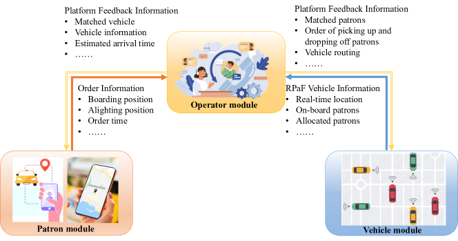
Figure 4: Interaction among three simulation modules. (Source of graphic illustration: https://www.freepik.com)

4.1 Operator module

The operator module is the core of the simulation. It employs the above-proposed operational algorithms to control or impact the actions of the other two modules, as illustrated in Figure 5. Specifically, the operator module dynamically (i) matches requests and vehicles (called the “matching algorithm”), (ii) dispatches vehicles to start transport service (“dispatching algorithm”), (iii) generates routing plans (“routing algorithm”), and (iv) relocates vehicles to meet the unserved demand (“repositioning algorithm”).

Note that each of the four types of algorithms may have several alternatives that have been proposed in the literature (Wang and Yang, 2019). Our module-based simulation environment can accommodate any specific algorithms of interest for study.

The operator module is also accountable for assessing the system’s performance. Based on information input from the other two modules, it computes metrics of interest, including patrons’ average trip time, total vehicle distance traveled, average occupancy of RPaF vehicles, etc.

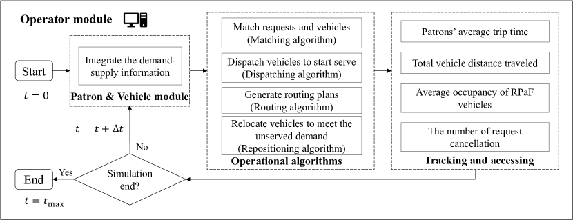
Figure 5: Simulation flow chart of the operator module (where $\Delta t$ is simulation timestamp).

4.2 Patron module

Patrons in this module are indexed by $i=1,2,...$ following the emergence order of their requests, and each is associated with a three-tuple state $r_{i}=\langle t_{i},\vec{l}_{i},\delta_{i}\rangle$, which are being updated at each simulation timestamp. Here, $t_{i}$ represents patron $i$’s request call-in timestamp, and vector $\vec{l}_{i}$ denotes her origin or destination location. For instance, $\vec{l}_{i}=(0,0)$ marks the connection point between the suburb and the freeway segment, as shown in Figure 1. The $\delta_{i}$ is an indicator variable, $\delta_{i}=0$ by default, meaning no match with any vehicles, $\delta_{i}=1$ if matched with a vehicle, $\delta_{i}=2$ if picked up by the designated vehicle, and $\delta_{i}=3$ if finished her trip.

The patron module simulates patrons’ behaviors in four stages, as shown in Figure 6:

1. Trip generation: Patrons are generated following specific temporal and spatial distributions.

2. Out-of-vehicle waiting: Patrons are put on wait at their origins (e.g., residential homes or the hub) until boarding.

3. In-vehicle riding: If a patron travels outbound, she first rides the vehicle to pick up other matched requests, if any are still waiting. And then, they ride together with the vehicle directly to the hub without any stops. The process is reversed for inbound patrons, who ride the vehicle first in a line-haul segment and then a tour for drop-offs. Note that the tour segments of pick-ups and drop-offs are separated to ensure patron acceptance.

4. Trip completion: Once patrons arrive at their destinations (the hub or residential places), they complete their trips and exit the simulation.

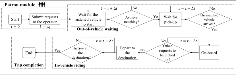
Figure 6: Simulation flow chart of patron module (where $\Delta t$ is simulation timestamp).

Patron $i$’s total trip time, $T_{i}$ [seconds], is recorded as the sum of the out-of-vehicle waiting time ($T^{w}_{i}$) and the in-vehicle riding time ($T^{r}_{i}$).

4.3 Vehicle module

We consider a fleet of $N$ identical vehicles, indexed by $n=1,...,N$, with capacity $C$ [seats/vehicle]. Each vehicle is attached with a four-tuple state $v_{n}=\langle o_{n},\vec{l}_{n},X_{n},\delta_{n}\rangle$. Here, $o_{n}$ denotes the vehicle occupancy (i.e., the number of on-board patrons); $\vec{l}_{n}$ represents the location of the vehicle; $X_{n}=\left\{i|x_{n,i}=1\&\delta_{i}=1,\right\}$ is the set of requests assigned to the vehicle $n$, where $x_{n,i}=1$ indicates a match between vehicle $n$ and patron $i$ and $x_{n,i}=0$ otherwise; and $\delta_{n}$ here indicates outbound service ($\delta_{n}=\text{`OB'}$) or inbound service ($\delta_{n}=\text{`IB'}$).

This module simulates the circulation of vehicles in bidirectional trips, as shown in Figure 7.

1. Outbound trip:

   1. Requests-accepting: Vehicles with $o_{n}=0$ and $|X_{n}|<u$ keep accepting request assignments from the matching algorithm (operator module). Each assignment updates the state of the matched patron with $\delta_{i}=1$ and adds the new matched request into $X_{n}$.

   2. Requests-collecting: Vehicles are dispatched by the dispatching algorithm (operator module) to pick up the matched requests in $X_{n}$. They follow the route planned by the routing algorithm (operator module). Upon each pick-up ($\vec{l}_{n}=\vec{l}_{i},i\in X_{n}$), the vehicle’s state is updated with an increment of $o_{n}+1$, and the patron’ state is also updated with $\delta_{i}=2$.

   3. Line-haul traveling: After collecting all matched requests (i.e., $o_{n}=u$ or $\delta_{i}=2,\forall i\in X_{n}$), the vehicle transports them directly to the hub without stops.

   4. Hub-unloading: Upon arrival at the hub, the outbound vehicle unloads all patrons ($\delta_{i}=3,\forall i\in X_{n}$) and then transitions to the inbound-service state ($\delta_{n}=\text{IB}$).

2. Inbound trip:

   1. Hub-loading: Inbound vehicles, assumed to follow a “stop-and-go” rule, load the waiting inbound patrons, if any, in a First-In-First-Out (FIFO) order. The vehicle state is changed to $\langle\tilde{o}_{n},\vec{l}_{n},X_{n},\text{IB}\rangle$, where $\tilde{o}_{n}\in[0,C]$ is the number of on-board inbound patrons, ensuring it does not exceed the vehicle capacity $C$ [seats/vehicle]; and the set $X_{n}$ contains inbound patrons onboard vehicle $n$.

   2. Line-haul traveling: If the number of onboard patrons $\tilde{o}_{n}>0$, the vehicle begins traveling directly to the first location in the tour made by the routing algorithm. Otherwise if $\tilde{o}_{n}=0$, the vehicle returns to the assigned location by the repositioning algorithm.

   3. Requests-delivering: The vehicle unloads patrons in $X_{n}$ following the plan by the routing algorithm. After dropping off the last patron, the vehicle, if not relocated, changes to the outbound-service state with $\delta_{n}=\text{OB}$; otherwise, it changes the state upon arrival to the repositioned location.

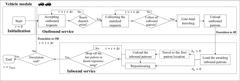
Figure 7: Simulation flow chart of vehicle module (where $\Delta t$ is simulation timestamp).

5 Experimental studies

5.1 Set-up

The experimental simulation’s baseline setting is as follows. The suburban area spans 5 km $\times$ 5 km, with a grid street network spaced by 0.1 km and a freeway segment of length $L=5$ km. All streets are two-way and have the same layout, e.g., three lanes in each direction. It is assumed that all intersections cause a standard delay of 10 seconds for vehicles passing through or making turns. Turning movements (including U-turns) can only be made at intersections. The RPaF vehicles are sedans with a maximum capacity of $C=4$ [seats/vehicle]. After a few rounds of tests, we set the initial fleet size to be $N=27$ [vehicles], so that at system steady states, the supply is generally balanced with the following demand.

We are particularly interested in the morning commute peak period when the demand is typically more aggregated than other periods and thus more crucial for the operation study. The total demand is set to be 180 and 20 patrons per hour for outbound and inbound directions, respectively. The corresponding densities in uniform demand distributions are $\lambda_{\rm OB}=7.2$ and $\lambda_{\rm IB}=0.8$ [patrons/sq. km/hour]. The emergence of requests follows Poisson processes.

We further consider non-uniform demand distributions using the following distance-decaying functions (Fan et al., 2024a),

$$\lambda_{\rm OB}(\vec{l})=\lambda_{\rm OB}\text{exp}(-\mu_{\rm OB}\|\vec{l}\|),\qquad\lambda_{\rm IB}(\vec{l})=\lambda_{\rm IB}\text{exp}(-\mu_{\rm IB}\|\vec{l}\|)$$ (11)

where $\vec{l}$ marks a location in the suburban region and $\|\vec{l}\|$ yields the distance to the freeway; and parameters $\mu_{\rm OB},\mu_{\rm IB}$ reflect the demand sensitivity to the distance, as shown in Figure 8, where they are set to be $\mu_{\rm OB}=\mu_{\rm IB}=0.1$. The $\lambda_{\rm OB}$ and $\lambda_{\rm IB}$ in Eq. (11) reflect the latent demand derived from the socio-economic characteristics of the suburb. Therefore, the above non-uniform distributions illustrate the influence of distance on actual demand, which has been noted in feeder systems (e.g., Fan et al., 2024a; Fan and Mei, 2018; Zhen and Gu, 2023).

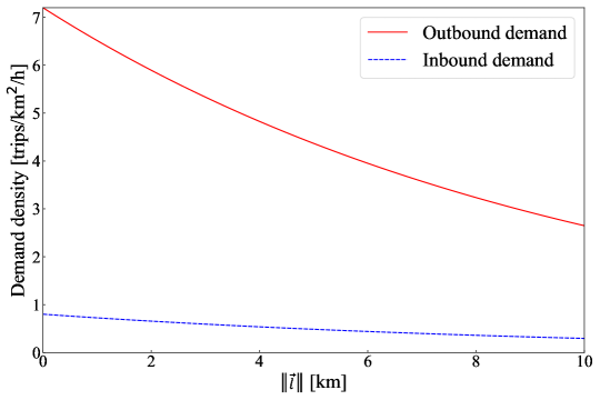
Figure 8: Non-uniform demand pattern (with $\mu_{\rm OB}=\mu_{\rm IB}=0.1$).

We begin by setting the occupancy target as $u=C=4$ and accordingly obtain the matching buffer distance $\Delta^{*}=1.67$ km for uniform demand scenarios by Eq. (8) in the Manhattan metric (since the street network is a grid network). As for non-uniform demand scenarios, the $\Delta^{*}$ is computed for each vehicle according to the local demand density.

The simulation runs for 2.5 hours, with a timestamp interval of $\Delta t=1$ second. The first 30 minutes serve as a warm-up period. Other parameter values are summarized in Table 2, which are adopted from previous studies (e.g., Kim et al., 2019; Daganzo and Ouyang, 2019b).

Table 2: Simulation parameter values.

Parameter	Baseline Value	Parameter	Baseline Value
$S,S^{{}^{\prime}}$ [km/hour]	$60,30$	$t_{d}$ [seconds/stop]	3
$\beta$ [$/hour]	20	$c_{f}$ [$/dispatch]	18
$\alpha$	0.5	$\bar{\tau}$ [hour]	0.1

For completeness, our simulation platform can also account for general trips that start and end within the suburb. To this end, we develop an algorithm based on Daganzo and Ouyang (2019b)’s Ride-Matching (RM) concept, which pools requests by matching their origins and destinations. Details are given in F. Note that the operational strategy of RM is fundamentally different from that of feeder services and should be independently operated with a dedicated fleet. Considering demand fluctuations may enhance operations with a shared fleet for both feeder and general services, but this is beyond the scope of this paper. Therefore, the subsequent analysis will exclusively focus on feeder services without explicitly exploring the general-trip service.

5.2 Evaluation of RPaF services

This section evaluates the performance of RPaF services. We begin by analyzing the impact of the zoning strategy (Section 5.2.1), which is a common strategy in feeder services (Fan et al., 2024a; Kim et al., 2019). Although the proposed algorithms work with or without zoning, we seek to understand its impact on overall system performance of the proposed RPaF. We then examine the effectiveness of the matching algorithm (Section 5.2.2), the dispatching algorithm (Section 5.2.3), and finally the repositioning algorithm (Section 5.2.4). The routing algorithm is not evaluated in detail as it is an implementation of the traditional TSP in specific street networks. Exact solutions to vehicle routing problems are typically found within 0.1 seconds for all simulated scenarios. For each evaluation, the performance metrics take an average of 50 runs with the same sequence of generated demand.

5.2.1 Zoning strategy

The zoning strategy partitions the entire service region into multiple zones and designates a fleet of vehicles serving specifically for each zone. It has proven effective in RPaF services (Fan et al., 2024a) and also in Flex-FBT systems (e.g., Kim et al., 2019). In contrast to those analytical studies based on idealized networks, we examine the effectiveness of zoning by simulations in specific street networks. However, we intend not to find the best partitions, which would be challenging and require further research (e.g., using graph-based network optimization). Instead, we divide the suburban region into four zones, as depicted in Figure 9 and 9. These zones are identical when facing uniform demand scenarios (Figure 9), but they differ when dealing with non-uniform demand scenarios (Figure 9). Inspired by Fan et al. (2024a), Zone 1/4 in Figure 9 is assigned the smallest/largest size due to the highest/lowest average demand density. Subsequently, we distribute the fleet of vehicles in proportion to the demand in each zone. Note that the results obtained from the current zone partition are somewhat conservative, and any enhancement in the zone partition could further improve the system’s performance.

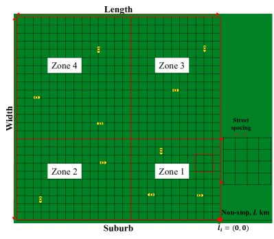
Figure 9: Zoning schemes under (a) uniform and (b) non-uniform demand scenarios.

Table 3 presents the performance of RFaF with and without zoning strategy under the baseline setting, showing the service rate and average trip time components for patrons. Here, the service rate refers to the percentage of patrons who have not canceled their requests and completed their trips in the feeder system. The findings demonstrate that the zoning strategy improves the service rate and decreases the trip time for patrons by up to 9.8%. However, the time savings are less apparent in non-uniform demand scenarios because most requests aggregate in zone 1 with short trip distances.

Table 3: Performance of RPaF with and without zoning under the baseline scenario.

Demand distribution	Zoning	Service rate∗ [%]	Waiting time [h]	In-vehicle time [h]	Trip time [h]
Uniform	With	91	0.12	0.25	0.37
	Without	90	0.15	0.26	0.41
Non-uniform	With	93	0.110	0.207	0.317
	Without	91.5	0.113	0.210	0.323

• ^∗ The service rate refers to the percentage of patrons who completed their trips without canceling requests.

We further conducted sensitivity analyses regarding inbound demand levels by scaling the baseline $\lambda_{\rm IB}$. The outbound demand is not chosen for analysis because it is theoretically proven to be irrelevant to zoning strategies in RPaF services (Fan et al., 2024a). Figures 10 and 11 illustrate the changes in service rates and patrons’ trip time savings. Specifically, Figures 10(a) and (b) show that higher demand levels can lead to increased service rates for RPaF with zoning, while RPaF without zoning will have lower service rates. Figure 11 indicates that patrons can achieve trip time savings over 11% in uniform demand scenarios, while non-uniform demand shows observable savings (e.g., over 3%) at lower demand levels.

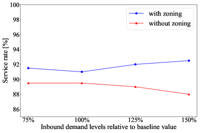
(a) Uniform demand scenarios

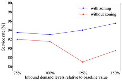
(b) Non-uniform demand scenarios

Figure 10: Service rates in RPaF with and without zoning.

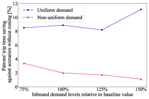
Figure 11: Patrons’ trip time savings against scenarios without zoning.

Nonetheless, we notice that as the inbound demand levels increase, some patrons at the hub may be unable to board the first departing vehicle due to the capacity limit and must continue waiting for the next one. We record the simulation instances of these patrons experiencing additional wait per hour and present the percentages as shown in Figure 12. The results reveal that while the percentage of leftover patrons is negligible at low demand levels, it steadily rises with increasing demand, remaining below 10% even at 1.5 times the baseline demand. In all simulation scenarios, we observe no patrons waiting for more than two vehicles to depart from the hub. In other words, all inbound patrons board either the first or second departing vehicle. It is worth noting that the above results are dictated by the supply of RPaF vehicles, which may mitigate the issue with a larger fleet size or vice versa.

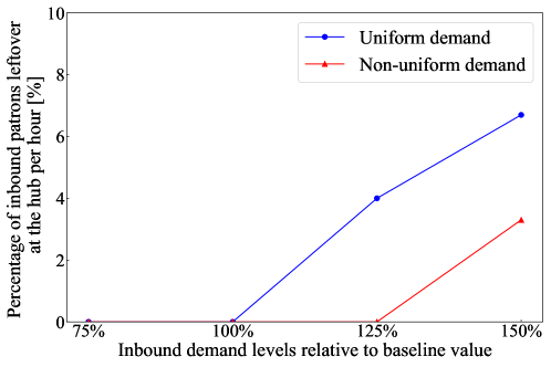
Figure 12: Percentage of inbound patrons leftover by the first departing vehicle at the hub per hour.

The zoning strategy remains in the following scenarios due to its benefits demonstrated above.

5.2.2 Matching algorithm

This section examines the effectiveness of the batch-based matching algorithm by comparing scenarios with and without the optimized matching buffer distance $\Delta^{*}$. For the latter, the (outbound) requests are always matched to the closest available vehicle within the same zone and no batch concept is employed.

Figures 13(a) and (b) depict service rates of RPaF across various outbound demand levels. It is evident that in both uniform and non-uniform demand scenarios, the optimized buffer distance helps RPaF enhance service rates, although the percentage declines as demand levels increase.

To enable a fair comparison, we increase the fleet size of the counterpart system to match the proposed system’s service rate of 90%. Table 4 summarizes the results under the baseline scenario, showing that the counterpart requires 14.8% and 12% more fleet, while patrons’ average trip time remains similar between the two systems.

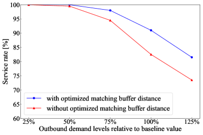
(a) Uniform demand scenarios

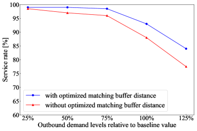
(b) Non-uniform demand scenarios

Figure 13: Service rates of RPaF with and without optimized matching buffer distance.

Table 4: Performance of RPaF with and without optimized matching buffer distance under the baseline scenario.

Demand distribution	Optimized matching buffer distance	Waiting time [h]	In-vehicle time [h]	Trip time [h]	Fleet size [vehicles]
Uniform	With	0.12	0.25	0.37	27
	Without	0.13	0.24	0.37	31
Non-uniform	With	0.12	0.21	0.33	25
	Without	0.13	0.20	0.33	28

5.2.3 Dispatching algorithm

The dispatching algorithms depend on the occupancy target $u$. This section examines hard- and soft-target strategies with $u\in\left\{2,3,4\right\}$. Table 5 shows the baseline scenario results, indicating that higher occupancy targets generally improve RPaF service rates for both dispatch algorithms. Furthermore, given the same occupancy targets, the hard-target algorithm achieves higher service rates and shorter average trip times for patrons compared to the alternative algorithm.

Table 5: Performance of RPaF with hard- and soft-target dispatching algorithms under the baseline scenario.

Demand distribution	Dispatching algorithm	Occupancy target $u$	Service rate [%]	Waiting time [h]	In-vehicle time [h]	Trip time [h]
Uniform	Hard-target	4	91	0.12	0.25	0.37
		3	85.5	0.11	0.24	0.35
		2	68	0.12	0.24	0.36
	Soft-target	4	79.5	0.13	0.25	0.38
		3	77	0.12	0.24	0.36
		2	64.5	0.12	0.24	0.36
Non-uniform	Hard-target	4	93	0.12	0.21	0.33
		3	86.5	0.12	0.20	0.32
		2	73	0.11	0.19	0.30
	Soft-target	4	82.5	0.12	0.21	0.33
		3	83	0.12	0.21	0.33
		2	70.5	0.11	0.20	0.31

The effect of varying demand levels is examined via sensitivity analyses while keeping all other factors the same as the baseline setting. Figures 14(a) and (b) depict the two dispatching algorithms’ percentage differences in patrons’ trip time, measured by $\left(1-\frac{\text{avg}\left(\left\{T^{\rm ST}_{i}\right\}\right)}{\text{avg}\left(\left\{T^{\rm HT}_{i}\right\}\right)}\right)\times 100\%$, where avg$(\cdot)$ returns the average of the argument, and the superscripts ST and HT indicate soft- and hard-target algorithms, respectively.

The findings suggest that under low demand levels, such as 25% of the baseline value, the soft-target algorithm can be more efficient, resulting in considerably shorter trip time for patrons, while the hard-target algorithm excels with medium to high demand levels. The result aligns with Fan et al. (2024b)’s finding in shuttle transit. Figure 14 also shows the impact of occupancy target $u$. It implies that inappropriate values of $u$ may invert the relative advantage/disadvantage relationship between the two dispatching strategies.

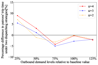
(a) Uniform demand scenarios

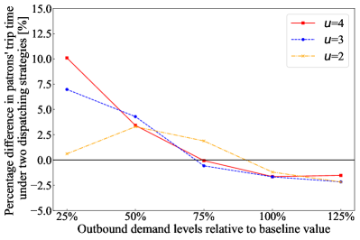
(b) Non-uniform demand scenarios

Figure 14: Percentage difference in patrons’ trip time under soft- and hard-target dispatching algorithms.

5.2.4 Repositioning algorithm

This section assesses the urgency concept in the repositioning algorithm. We compare the baseline setting (i.e., $\alpha=0.5$ in Eq. (10)) with two alternative repositioning algorithms: one prioritizing only requests’ unmatched time (i.e., $\alpha=1$) and the other focusing solely on the unmatched requests’ distance to the vehicle (i.e., $\alpha=0$).

Table 6 presents the baseline scenario results for repositioning algorithms with $\alpha=1,0.5,0$. While their differences in service rates and patrons’ trip time components are small under uniform demand scenarios, they can be notable in non-uniform scenarios. For instance, the service rate of RPaF with $\alpha=0.5$ exceeds that with $\alpha=1$ by over 4%. The outcome highlights the importance of selecting an appropriate $\alpha$ value in balancing unmatched requests’ waiting times and distance to available vehicles.

Table 6: Performance of RPaF with varying repositioning algorithms under the baseline scenario.

Demand distribution	Parameter $\alpha$	Service rate [%]	Waiting time [h]	In-vehicle time [h]	Trip time [h]
Uniform	0	90	0.12	0.25	0.37
	0.5	91	0.12	0.25	0.37
	1	90.5	0.13	0.25	0.38
Non-uniform	0	89.5	0.11	0.21	0.32
	0.5	93	0.12	0.21	0.33
	1	88.5	0.12	0.21	0.33

5.3 Comparison with two counterpart feeder services

We now start comparing the proposed RPaF with two counterpart feeder services: (i) the Ride-Sharing as Feeder (RSaF) (Daganzo and Ouyang, 2019a; Liu and Ouyang, 2021), and (ii) the Flexible-Route Feeder-Bus Transit (Flex-FBT) (Chang and Schonfeld, 1991b; Kim et al., 2019). The core distinction among them lies in their matching and dispatching mechanisms as illustrated in Figure 15.

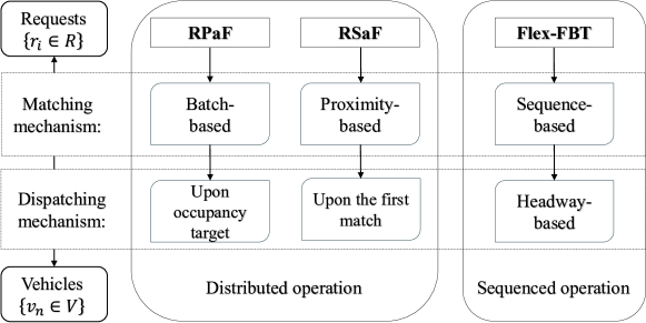
Figure 15: Schematic diagrams of matching and dispatching mechanisms in RPaF, RSaF, and Flex-FBT services.

Nevertheless, the studies on RSaF and Flex-FBT are mostly analytical system designs under idealized assumptions (e.g., spatially uniform demand distribution). For comparability, we devise simulation processes according to their operational characteristics, as given below:

1. The RSaF does not pool requests but instantly matches and dispatches the available vehicle to pick up the nearest (outbound) request. The vehicle, en route to the initial request, remains available to receive new request assignments until the first passenger boards or the number of assignments reaches the occupancy target $u$. (Thus, we have $o_{n}\leq u,\forall n$.) If multiple requests are matched to the vehicle, it follows a proximity-based routing rule (rather than the TSP plan as in our RPaF), by which it always visits the next closest point. The inbound operation of RSaF is identical to the proposed RPaF.

2. Flex-FBT dispatches vehicles at regular headways and matches the (outbound) requests within each headway to the successive vehicles. The routing of vehicles follows the optimal TSP-tour plan.

All parameter values of the two systems, without being explicitly mentioned, are maintained at the baseline setting. The simulation steps of RSaF and Flex-FBT are outlined in C and D, respectively. The following comparisons evaluate the three systems’ performance regarding service rates, patrons’ average trip times, and fleet sizes.

Figures 16(a) and (b) display the service rates of three feeder services under uniform and non-uniform demand scenarios, respectively. As expected, their service rates increase with fleet size. However, for the same fleet size, RPaF and Flex-FBT demonstrate higher service rates than RSaF, due to their greater transportation efficiency.

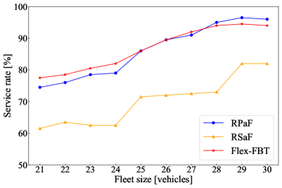
(a) Uniform demand scenarios

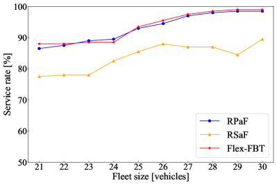
(b) Non-uniform demand scenarios

Figure 16: Service rates of RPaF, RSaF, and Flex-FBT under the baseline scenario.

Table 7 summarizes the results for three feeder systems operating at the same service rate, i.e., 90%. It is not surprising that RSaF requires the largest fleet sizes across most demand scenarios. For patrons in RSaF, however, they enjoy shorter average trip times than those in the other two alternatives. The opposite is Flex-FBT, which usually operates smaller fleet sizes but yields the longest average trip times. The performance of RPaF sits in between. It produces average trip times in the neighborhood of RSaF’s while utilizing fewer fleets.

Table 7: Performance of RPaF, RSaF, Flex-FBT at service rate of 90%.

Demand distribution	OB demand levels relative to baseline	Trip time [h]			Fleet size [vehicles]
		RPaF	RSaF	Flex-FBT	RPaF	RSaF	Flex-FBT
Uniform	25%	0.39	0.31	0.57	15	19	12
	50%	0.40	0.29	0.55	19	28	18
	75%	0.38	0.32	0.54	24	30	24
	100%	0.38	0.33	0.55	27	33	27
	125%	0.38	0.35	0.54	32	34	36
Non-uniform	25%	0.34	0.25	0.50	14	18	10
	50%	0.33	0.26	0.46	16	25	15
	75%	0.33	0.28	0.46	20	27	19
	100%	0.33	0.29	0.46	25	32	25
	125%	0.33	0.30	0.45	29	33	33

6 Real case study

This section illustrates an application of the proposed RPaF system in a real city, i.e., New York City, USA. The study area occupies the uptown area of Manhattan, roughly 19.9 sq. km, as shown in Figure 17(a). We retrieve the street network from the OpenStreetMap (https://www.openstreetmap.org). The network contains 11,503 roadway links and 7,725 intersections. The related network configurations include the length, number of lanes, and average speed of each link, the control types and signal plans (if signalized) of each intersection, one-way streets, turn restrictions, etc.

The demand data is sourced from the New York City Taxi Public Dataset (NYC Taxi and Limousine Commission, 2014). We extracted the morning-peak trip data (from 7 to 9 a.m.) of green taxis on March 2, 2014. We filter the data with trip ends between uptown Manhattan and a subway transfer station at 96 St LB LC, midtown (where two subway lines intersect). Figures 17(b) and Figure 17(c) visualize outbound and inbound demand, respectively. During the 2-hour study period, there are 321 records of requests (289 for outbound and 32 for inbound). According to the clusters of demand, we partition service zones as shown in Figure 17(d).

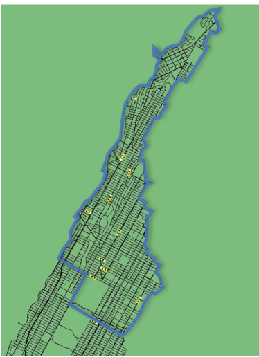
(a) Research area (19.9 sq. km)

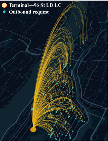
(b) Outbound demand flow

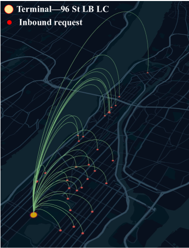
(c) Inbound demand flow

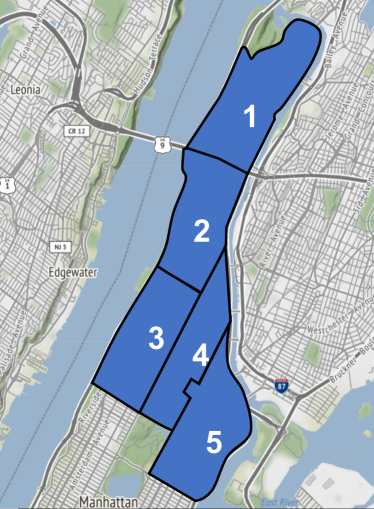
(d) Zoning scheme

Figure 17: Visualization of the Manhattan road network and demand data.

We compare three new feeder systems (i.e., RPaF, RSaF, and Flex-FBT) with the existing non-shared taxi service. Figure 18 gives the service rates of the four systems with varying fleet sizes. The results imply that all new systems perform better transportation efficiency (with considerably higher service rates per hour) than the existing non-shared taxis. The relationship among RPaF, RSaF, and Flex-FBT aligns with the previous findings.

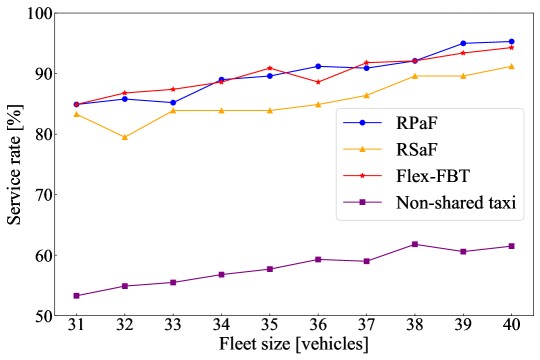
Figure 18: Service rates of RPaF, RSaF, Flex-FBT, and non-shared taxis with varying fleet sizes.

We next scale the current demand data from 25% to 200%. For each demand scenario, we adjust the fleet sizes of the three new systems to maintain a service rate of 90%. The non-shared taxi’s fleet size is set to 100 vehicles in all scenarios, ensuring a service rate close to 100% at current or lower demand levels. This makes our comparison conservative, and the results are summarized in Table 8.

We have several new findings. First, taxi trips consistently have the shortest average travel time. However, their service rate declines significantly as demand increases, leading to a substantial market gap — up to 34% (i.e., $100\%-66\%$) when demand reaches 200% of current levels. Second, RSaF demonstrates strong competition with taxis at low demand levels, adding only 0.04 hours (2.4 minutes) per patron while operating about 60 fewer vehicles. Third, RPaF shows improved performance at higher demand levels, exhibiting negligible differences in average trip time compared to RSaF, while achieving a reduction in fleet size by eight vehicles. Lastly, Flex-FBT appears less competitive against other systems since it produces significantly longer average trip times for patrons in all scenarios.

Table 8: Performance of RPaF, RSaF, Flex-FBT in Manhattan network at service rate of 90%.

OB demand levels relative to baseline	Trip time [h]				Fleet size [vehicles]
	Non-shared taxi*	RPaF	RSaF	Flex-FBT	RPaF	RSaF	Flex-FBT
25%	0.40 (100%)	0.58	0.44	0.78	23	30	20
50%	0.42 (100%)	0.59	0.46	0.78	29	34	28
75%	0.40 (99%)	0.59	0.53	0.85	33	36	32
100%	0.40 (94%)	0.60	0.55	0.83	36	40	35
125%	0.40 (85%)	0.60	0.56	0.86	39	45	41
…	…	…	…	…	…	…	…
200%	0.47 (66%)	0.61	0.60	0.87	55	63	59

• The fleet size of non-shared taxis is set to 100 vehicles and the number in parentheses indicates service rates corresponding to this fleet size.

7 Conclusion

This paper studies Ride-Pooling as Feeder (RPaF) services, whose distinct operation characteristics motivate us to investigate the potential for lowering system costs in a dynamic, door-to-door routing environment. Specifically, we customize three novel algorithms for vehicle-request matching, vehicle dispatching, and repositioning operations. Analytical analysis is utilized to optimally parameterize the algorithms concerning for example the number of pooling requests and matching buffer distance. An open-source microscopic simulation platform is developed for studying RPaF with the proposed algorithms.

We have conducted extensive experiments in morning-peak scenarios to verify the effectiveness of the proposed operation algorithms across varying demand levels and uniform and non-uniform distribution patterns. The performance of RPaF is further compared with two counterparts, namely the Ride-Sharing as Feeder (RSaF) and Flexible-Route Feeder-Bus Transit (Flex-FBT). The results show that RPaF generally performs better under medium to high demand levels, producing higher service rates with the same fleet size or fewer fleet sizes with comparative average trip times for patrons as compared to its counterparts. The divergent performance between Flex-FBT and RP/RSaF is notable and may stem from their fundamentally different operational mechanisms, i.e., the so-called sequenced and distributed operation (see descriptions in Section 1 and illustration in Figure 15). Lastly, we demonstrate the application of RPaF in a real-world study of the uptown Manhattan street network (New York City, USA) using actual taxi trip data. Overall, RPaF shows great potential as an effective feeder system, balancing well the level of service (in terms of service rate and patrons’ average trip time) and operational costs (related to fleet size) under the proper conditions.

It is worth noting that the current study contains some limitations that warrant future investigation. First, we did not consider riders’ socio-economic heterogeneity, such as varying values of time and diverse preferences, which do exist in reality but require high-quality survey data to unveil. Once available, these factors can be incorporated more readily into the simulation platform than in the previous analytical models. To this end, advanced matching and routing algorithms should be developed based on TSP or VRP (Vehicle Routing Problem) with time window constraints (Santi et al., 2014). In dynamic contexts, solution efficiency is crucial to these algorithms. Second, the suggested zoning strategy is contingent upon the availability of parking resources at the hub, which poses practical challenges, as authorities must also address the demands of private vehicle use and cycling. Achieving an efficient and equitable parking allocation requires further investigation into the diverse needs of all stakeholders. Third, we have set the vehicles in all service zones to be identical. In contrast, a fleet of mixed-size vehicles may benefit the operation during different periods and for service zones with different distances to the hub. Forth, driver noncompliance issues are also worth exploring, particularly through incentive-based approaches (Qian et al., 2017; Guda and Subramanian, 2019). Fifth, operational issues in non-equilibrium RPaF systems also deserve attention due to constantly increasing/decreasing demand and significant spatial imbalances. In this regard, insights from previous studies on non-shared ride-sourcing mobility (e.g., Ramezani and Nourinejad, 2018; Nourinejad and Ramezani, 2020; Ramezani and Valadkhani, 2023; Valadkhani and Ramezani, 2023) may guide the development of solutions for dynamic and imbalanced RPaFs. Lastly, expanding the single-hub system to transit networks fed by RPaFs certainly merits further exploration. It is intriguing to see how much city-wide benefit such integrated systems could bring.

Appendix A Lists of abbreviations and notations

Abbreviations and notations used in this paper are summarized in Table 1 and 2, respectively.

Table 1: Abbreviations

Abbreviation	Description
AV	Autonomous vehicle
DAR, DARP	Dial-a-ride, dial-a-ride problem
DAT	Demand adaptive transit
Fix-FBT	Fixed-route feeder bus transit
Flex-FBT	Flexible-route feeder bus transit
M2M, M2O, O2M	Many to many, many to one, one to many
MAST	Mobility allowance shuttle transit
ODSR	On-demand shared-ride
ODT	On-demand transit
P2P-RSaF	Peer-to-peer ride-sharing as feeder
RP	Ride-pooling
RPaF	Ride-pooling as feeder
RP-HD	Ride-pooling with hold-dispatch strategy
RSaF	Ride-sharing as feeder
Semiflex-FBT	Semi-flexible feeder bus transit
SAVaF	Shared autonomous vehicle as feeder
STaF	Shared taxi as feeder
TNC	Transportation network company
TSP	Traveling salesman problem

Table 2: List of notations

Variables, sets, parameters	Description	Unit
Variables
$U$	Pooling target for the number of requests	patrons
$\Delta$	Matching buffer distance	km
Patron’s set $R\equiv\{r_{i}=\langle t_{i},\vec{l}_{i},\delta_{i}\rangle\}$
$\tau_{i}$	Patron $i$’s request call-in timestamp	/
$\vec{l}_{i}$	Patron $i$’s location	/
$\delta_{i}$	Patron $i$’s indicator variable	/
Unmatched requests set $\widetilde{X}_{0}$
Vehicle’s set $V\equiv\{v_{n}=\langle o_{n},\vec{l}_{n},X_{n},\delta_{n}\rangle\}$
$o_{n}$	Outbound vehicle $n$’s occupancy	patrons/vehicle
$\tilde{o}_{n}$	Inbound vehicle $n$’s occupancy	patrons/vehicle
$\vec{l}_{n}$	Vehicle $n$’s location	/
$X_{n}$	The set of requests assigned to the vehicle $n$	/
$\delta_{n}$	Vehicle $n$’s indicator variable	/
Parameters
$c_{f}$	Operational cost per dispatch	$/dispatch
$C$	Vehicle capacity	seats/vehicle
$k$	Constant parameter in TSP-tour length formula	/
$u$	Vehicle occupancy target	patrons/vehicle
$L$	Line haul distance	km
$N$	Fleet size	vehicles
$S,S^{{}^{\prime}}$	Vehicle speed on the freeway and suburban streets	km/h
$S^{{}^{\prime}}(u)$	Vehicle commercial speed in TSP tours	km/h
$t_{d}$	Vehicle delay	seconds
$T_{i},T_{i}^{w},T_{i}^{r}$	Average trip time components of patron $i$	seconds
$\lambda_{\text{OB}},\lambda_{\text{IB}}$	Demand density of outbound and inbound patrons	trips/$\text{km}^{2}$/h
$\beta$	Patrons’ value of time (VOT)	$/hour/patron
$\eta$	Parameter in inbound vehicles’ trip distance formula	/
$\bar{\tau}$	Patrons’ maximum tolerance time	minutes

Appendix B Proof to Eq. (3)

Let $D$ be the distance of the random request to the center (i.e., the location of the vehicle) of the area of $A(\Delta)$. The $D$ is i.i.d. and uniformly distributed in the range of $[0,\Delta]$. The $U$ points of $D$ divide the range into $U+1$ segments, and the distance between the $u$-th closest point to the center will be $\frac{u}{U+1}\Delta$, which defines an area of $\left(\frac{u}{U+1}\right)^{2}A(\Delta)$. In this area, the expected TSP-tour distance of visiting $u$ points is

$$k\sqrt{A(\Delta)u}\frac{u}{U+1},$$ (1)

which yields Eq. (3) by dividing the commercial speed $S^{\prime}(u)$.

Appendix C Pseudo-code of RSaF

For comparability, we set RSaF vehicles’ occupancy target as $u=4$ identical to our RPaF’s. Note that in the original theoretical studies (Daganzo and Ouyang, 2019a; Liu and Ouyang, 2021), RSaF was restricted to cases of $u=2$ for the sake of traceability in solving multiple equations of states, whose number grows quadratically with $u$. Yet, expanding our simulation platform to accommodate higher $u$ values is much simpler. The following provides the pseudo-code for simulating RSaF.

  Algorithm 4 Simulation of RSaF

    Input: Requests set $R\equiv\{r_{i}=\langle t_{i},\vec{l}_{i},\delta_{i}\rangle\}$, vehicles set $V\equiv\{v_{n}=\langle o_{n},\vec{l}_{n},X_{n},\delta_{n}\rangle\}$, Simulation maximum time $t_{\text{max}}$, simulation time step $\Delta t$.

1:Set simulation time step $t=0$.

2:while $t\leq t_{\text{max}}$ do

3:     Initialization:

4:     if $t=0$ then

5:         Any vehicle $n$ goes to the initial located position, awaiting assignment.      

6:     Matching:

7:     if $t$ reach $\Delta t$ then

8:         Apply the proximity-based principle to output vehicle-demand mapping dictionary $\mathbf{X}=\{X_{n}\}$.      

9:     for each zone do

10:         Iterate over vehicles and send commands:

11:         for each vehicle $n$ in vehicle set $V$ do

12:              Outbound service:

13:              if $v_{n}=\langle o_{n}=0,\vec{l}_{n},X_{n}=\emptyset,\text{OB}\rangle$ state then

14:                  Vehicle $n$ remains in its initial state and stays stationary.

15:              else if $v_{n}=\langle o_{n}=0,\vec{l}_{n},X_{n}\neq\emptyset,\text{OB}\rangle$ state then

16:                  Vehicle $n$ departs to pick up the first patron.

17:              else if $v_{n}=\langle o_{n}=1,\vec{l}_{n},X_{n},\text{OB}\rangle$ state then

18:                  The first patron is already on board.

19:                  Vehicle $n$ stops matching.

20:                  if $X_{n}=\emptyset$ then

21:                       Vehicle $n$ goes directly to the hub.

22:                  else if $X_{n}\neq\emptyset$ then

23:                       Vehicle $n$ picks up other matched requests $X_{n}$, and finally returns to the hub.                   

24:              else if vehicle $n$ arrives at the hub then

25:                  Outbound patrons alight.

26:                  Inbound service:

27:                  $v_{n}\leftarrow v_{n}=\langle\tilde{o}_{n},\vec{l}_{n},X_{n},\delta_{n}=\text{IB}\rangle$.

28:                  if $\tilde{o}_{n}=0$ then

29:                       Vehicle $n$ returns the last patron pick-up position $\vec{l}^{{}^{\prime}}$ in the outbound service.

30:                  else if $\tilde{o}_{n}>0$ then

31:                       Vehicle $n$ sends inbound patrons back to the suburbs under the routing algorithm until the last drop-off position $\vec{l}^{{}^{\prime}}$.                   

32:              else if $v_{n}=\langle\tilde{o}_{n}=0,\vec{l}_{n}=\vec{l}^{{}^{\prime}},X_{n}=\emptyset,\text{IB}\rangle$ then

33:                  $v_{n}\leftarrow v_{n}=\langle o_{n},\vec{l}_{n},X_{n},\delta_{n}=\text{OB}\rangle$.                             

34:     if all patrons have been served then

35:         break      

36:     $t=t+\Delta t$.

 

Appendix D Pseudo-code of Flex-FBT

The headway of Flex-FBT, denoted by $h$, is optimized using the models in Appendix D of Fan et al. (2024a), set to 9.42 minutes under the baseline setting and updated for every other scenario. The detailed optimization models are omitted for brevity. The pseudo-code for simulating Flex-FBT is provided below.

  Algorithm 5 Simulation of Flex-FBT

    Input: Requests set $R\equiv\{r_{i}=\langle t_{i},\vec{l}_{i},\delta_{i}\rangle\}$, vehicles set $V\equiv\{v_{n}=\langle o_{n},\vec{l}_{n},X_{n},\delta_{n}\rangle\}$, simulation maximum time $t_{\text{max}}$, fleet size $N$, vehicle capacity $C$, optimal headway $h$, simulation time step $\Delta t$, number of sub-areas $A$.

1:Initialization:

2:Set simulation time step $t=0$.

3:Set initial departure time $t_{p}=h$.

4:Define $R_{\text{OB}}=\emptyset$ as the set of outbound patrons to be matched in the suburb.

5:Define $R_{\text{IB}}=\emptyset$ as the set of inbound patrons waiting at the hub.

6:while $t\leq t_{\text{max}}$ do

7:     for each zone id $a\in\{1,...,A\}$ do

8:         Renew $V^{(a)}=\{v_{n}\}$, $R^{(a)}_{\text{OB}}$, $R^{(a)}_{\text{IB}}$.

9:         if $|V^{(a)}|<N^{(a)}$, where $|\cdot|$ represents the number of service vehicles in zone $a$ then

10:              if $R^{(a)}_{\text{IB}}=\emptyset$ then

11:                  No inbound requests:

12:                  if $|R^{(a)}_{\text{OB}}|\geq C$ then

13:                       Reach full match:

14:                       Filter the first $\text{min}\{C,|R^{(a)}_{\text{OB}}|\}$ elements in $R^{(a)}_{\text{OB}}$ and determine them be set $X_{n}$.

15:                       Dispatch vehicle $n$ with state $v_{n}=\langle\tilde{o}_{n}=0,\vec{l}_{n},X_{n},\delta_{n}=\text{OB}\rangle$.

16:                       Vehicle $n$ picks up matched outbound requests under the instructions of the routing algorithm and finally returns to the hub.

17:                       $V^{(a)}\leftarrow V^{(a)}\cup v_{n}$.

18:                  else if $t$ reach $t^{(a)}_{p}$ and $R^{(a)}_{\text{OB}}\neq\emptyset$ then

19:                       Reach departure interval:

20:                       $X_{n}=R^{(a)}_{\text{OB}}$.

21:                       Dispatch vehicle $n$ with state $v_{n}=\langle\tilde{o}_{n}=0,\vec{l}_{n},X_{n},\delta_{n}=\text{OB}\rangle$.

22:                       Vehicle $n$ picks up matched outbound requests under the instructions of the routing algorithm and finally returns to the hub.

23:                       $V^{(a)}\leftarrow V^{(a)}\cup v_{n}$.                   

24:                  $t^{(a)}_{p}=t+h$.

25:              else if $R^{(a)}_{\text{IB}}\neq\emptyset$ then

26:                  Have inbound requests:

27:                  Filter the first $\text{min}\{C,|R^{(a)}_{\text{IB}}|\}$ elements in $R^{(a)}_{\text{IB}}$ and let them be Set $X_{\rm IB}$.

28:                  if $|R^{(a)}_{\text{OB}}|\geq C$ then

29:                       Reach full match:

30:                       Filter the first $\text{min}\{C,|R^{(a)}_{\text{OB}}|\}$ elements in $R^{(a)}_{\text{OB}}$ and determine them be set $X_{\rm OB}$.

31:                       Dispatch vehicle $n$ with state $v_{n}=\langle\tilde{o}_{n}>0,\vec{l}_{n},X_{n}=X_{\rm IB}\cup X_{\rm OB},\delta_{n}\rangle$.

32:                       Generate inbound route $\Upsilon_{\text{IB}}$ based on $X_{\rm IB}$; and generate outbound route $\Upsilon_{\text{OB}}$ based on $X_{\rm OB}$.

33:                       Vehicle $n$ ($\delta_{n}=\text{IB}$) first delivers inbound patrons along the inbound route $\Upsilon_{\text{IB}}$; then switches state ($\delta_{n}=\text{OB}$) to pick up outbound patrons along the outbound route $\Upsilon_{\text{OB}}$; and finally returns to the hub.

34:                       $V^{(a)}\leftarrow V^{(a)}\cup v_{n}$.

35:                  else if $t$ reach $t^{(a)}_{p}$ and $R^{(a)}_{\text{OB}}\neq\emptyset$ then

36:                       Reach departure interval:

37:                       $X_{\rm OB}=R^{(a)}_{\text{OB}}$

38:                       Dispatch vehicle $n$ with state $v_{n}=\langle\tilde{o}_{n}>0,\vec{l}_{n},X_{n}=X_{\rm IB}\cup X_{\rm OB},\delta_{n}=\text{IB}\rangle$.

39:                       Generate inbound route $\Upsilon_{\text{IB}}$ based on $X_{\rm IB}$; and generate outbound route $\Upsilon_{\text{OB}}$ based on $X_{\rm OB}$.

40:                       Vehicle $n$ ($\delta_{n}=\text{IB}$) first delivers inbound patrons along the inbound route $\Upsilon_{\text{IB}}$; then switches state ($\delta_{n}=\text{OB}$) to pick up outbound patrons along the outbound route $\Upsilon_{\text{OB}}$; and finally returns to the hub.

41:                       $V^{(a)}\leftarrow V^{(a)}\cup v_{n}$.                   

42:                  $t^{(a)}_{p}=t+h$.                        

43:         for each vehicle $n$ in vehicle set $V^{(a)}$ do

44:              if vehicle $n$ returns to hub then

45:                  Renew $V^{(a)}\leftarrow V^{(a)}\setminus\{v_{n}\}$.                             

46:     if all patrons have been served then

47:         break.      

48:     $t=t+\Delta t$.

 

Appendix E Open-tour TSP model

We employ the classic open-tour TSP model (2) to generate the optimal route for visiting $|X_{n}|$ request points for any vehicle $n$ (Sengupta et al., 2019; Singamsetty et al., 2021). We acquire the match set $X_{n}$ as input to the model. The current location of vehicle $n$ is represented by $\vec{l}_{n}$, and the locations of all matched requests are $\{\vec{l}_{i\in X_{n}}\}$. They together constitute the set of to-be-visit points, denoted $\Theta$ (where subscript $n$ is dropped without confusion). The total number of points in the set is thus $\theta=|\Theta|\leq|X_{n}|+1$, which takes the equality sign when $\vec{l}_{n}$ does not overlap with any of $\{\vec{l}_{i\in X_{n}}\}$. Additionally, we retrieve the travel distances or costs between the points, denoted $\{c_{ij}:i,j\in\Theta\}$, from the simulation environment.

We introduce: binary decision variables $\{x_{ij}\in\{0,1\}:i,j\in\Theta\}$, where $x_{ij}=1$ means the edge $(i,j)$ is included in the tour, and otherwise $x_{ij}=0$; and auxiliary decision variables $\{d_{k}:k\in\Theta\}$, where $d_{k}=-1$ denotes the start point, $d_{k}=+1$ the endpoint, and $d_{k}=0$ intermediate points. Since the start point is known, we can stipulate the rest $d_{k}$ as binary variables and enforce that their sum is equal to 1 (Rasmussen, 2011). Therefore, the open-tour TSP can be constructed to minimize the total distance or cost, as given by

$$\operatorname*{minimize}_{\{x_{ij}\},\{d_{k}\}} \quad\sum_{i=1}^{\theta}\sum_{j=1}^{\theta}c_{ij}x_{ij},$$ (2a)

subject to:

$$\quad\sum_{i=1}^{\theta}x_{ij}=1,\quad\forall j>1,j\in\Theta,$$ (2b)

$$\quad\sum_{i=1}^{\theta}x_{ik}-\sum_{j=1}^{\theta}x_{kj}=d_{k},\quad\forall k\in\Theta,$$ (2c)

$$\quad d_{1}=-1,\sum_{k=2}^{\theta}d_{k}=1,$$ (2d)

$$\quad\sum_{i\in M}\sum_{j\in M}x_{ij}\leq|M|-1,\quad\forall M\subset\Theta,2\leq|M|\leq\theta-2,$$ (2e)

$$\quad x_{ij}\in\{0,1\},\quad\forall i,j\in\Theta,$$ (2f)

$$\quad d_{k}\in\{0,1\},\quad\forall k>1,k\in\Theta,$$ (2g)

where constraints (2b) ensure each point is visited once; constraints (2c) guarantee that the vehicle leaves from the start point, visits all intermediate points, and finishes at the endpoint; constraint (2d) ensures the open tour, meaning the vehicle does not return to the start point; constraint (2e) avoids subtours; and constraints (2f) and (2g) define the valid range of decision variables.

Appendix F Operational algorithm for general trips completed within the suburb

For illustration, Figure 1 depicts a Ride-Matching (RM) scenario between two riders, namely Seeker and Taker. Without loss of generality, the vehicle is assumed to travel horizontally first, followed by a vertical movement. Within the service zone $R$, assume that Seeker boarded the vehicle at point O and traveled $z$ km to reach the current location C. The sub-region formed by points C and D is defined as $R_{1}$, while the sub-region formed by D and the boundary of $R$ is defined as $R_{2}$. To identify a valid RM, we verify Taker’s Origin-Feasibility (OF) and Destination-Feasibility (DF) based on two criteria: (i) Taker can be picked up within her maximum tolerance time $\bar{\tau}$, and (ii) for combined trips, neither rider requires a detour.

The steps of RM operation are detailed in Algorithm F:

  Algorithm 6 Ride-Matching algorithm for general trips

  Input: Vehicle speed $S^{\prime}$, matching tolerance time $\bar{\tau}$.

1:Attain OD information (O, D) and current location C of Seeker.

2:while the horizontal distance $z$ traveled by the vehicle is less than the horizontal distance between D and O, denoted $X$ do

3:     New request arises (Taker).

4:     The origin and destination of the Taker are A and B, respectively.

5:     Initialization:

6:     OF, DF = False, False

7:     Check Origin-Feasibility (OF):

8:     if the Manhattan distance between A and C is less than or equal to $\bar{\tau}S^{\prime}$ (i.e. A is located in the isosceles right triangle area) then

9:         OF=True      

10:     Check Destination-Feasibility (DF):

11:     if B is located in the upper right of A in the region $R_{1}$ or in the region $R_{2}$ then

12:         DF=True      

13:     Check valid ride-matching:

14:     if OF && DF == True then

15:         Seeker and Taker are successfully matched.      

 

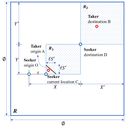
Figure 1: Illustration of Ride-Matching for general trips (Daganzo and Ouyang (2019b))

References

- Adebisi and Hurdle (1982) Adebisi, O., Hurdle, V., 1982. Comparing fixed-route and flexible-route strategies for intraurban bus transit. Transportation Research Record .
- Agatz et al. (2012) Agatz, N., Erera, A., Savelsbergh, M., Wang, X., 2012. Optimization for dynamic ride-sharing: A review. European Journal of Operational Research 223, 295–303.
- Aldaihani and Dessouky (2003) Aldaihani, M., Dessouky, M.M., 2003. Hybrid scheduling methods for paratransit operations. Computers & Industrial Engineering 45, 75–96.
- Aldaihani et al. (2004) Aldaihani, M.M., Quadrifoglio, L., Dessouky, M.M., Hall, R., 2004. Network design for a grid hybrid transit service. Transportation Research Part A: Policy and Practice 38, 511–530.
- Alonso-Mora et al. (2017) Alonso-Mora, J., Samaranayake, S., Wallar, A., Frazzoli, E., Rus, D., 2017. On-demand high-capacity ride-sharing via dynamic trip-vehicle assignment. Proceedings of the National Academy of Sciences 114, 462–467.
- Badia and Jenelius (2021) Badia, H., Jenelius, E., 2021. Design and operation of feeder systems in the era of automated and electric buses. Transportation Research Part A: Policy and Practice 152, 146–172.
- Bian and Liu (2019a) Bian, Z., Liu, X., 2019a. Mechanism design for first-mile ridesharing based on personalized requirements part i: Theoretical analysis in generalized scenarios. Transportation Research Part B: Methodological 120, 147–171.
- Bian and Liu (2019b) Bian, Z., Liu, X., 2019b. Mechanism design for first-mile ridesharing based on personalized requirements part ii: Solution algorithm for large-scale problems. Transportation Research Part B: Methodological 120, 172–192.
- Calabrò et al. (2023) Calabrò, G., Araldo, A., Oh, S., Seshadri, R., Inturri, G., Ben-Akiva, M., 2023. Adaptive transit design: Optimizing fixed and demand responsive multi-modal transportation via continuous approximation. Transportation Research Part A: Policy and Practice 171, 103643.
- Ceder (2013) Ceder, A., 2013. Integrated smart feeder/shuttle transit service: simulation of new routing strategies. Journal of Advanced Transportation 47, 595–618.
- Chan and Shaheen (2012) Chan, N.D., Shaheen, S.A., 2012. Ridesharing in north america: Past, present, and future. Transport reviews 32, 93–112.
- Chandra and Quadrifoglio (2013) Chandra, S., Quadrifoglio, L., 2013. A model for estimating the optimal cycle length of demand responsive feeder transit services. Transportation Research Part B: Methodological 51, 1–16.
- Chang and Schonfeld (1991a) Chang, S.K., Schonfeld, P.M., 1991a. Integration of fixed-and flexible-route bus systems. Transportation Research Record .
- Chang and Schonfeld (1991b) Chang, S.K., Schonfeld, P.M., 1991b. Optimization models for comparing conventional and subscription bus feeder services. Transportation Science 25, 281–298.
- Chen and Schonfeld (2022) Chen, L., Schonfeld, P., 2022. Optimized zone sizes and headways for flexible-route bus services—a two zone case. KSCE Journal of Civil Engineering 26, 3136–3149.
- Chen and Nie (2017a) Chen, P.W., Nie, Y.M., 2017a. Analysis of an idealized system of demand adaptive paired-line hybrid transit. Transportation Research Part B: Methodological 102, 38–54.
- Chen and Nie (2017b) Chen, P.W., Nie, Y.M., 2017b. Connecting e-hailing to mass transit platform: Analysis of relative spatial position. Transportation Research Part C: Emerging Technologies 77, 444–461.
- Chen and Nie (2018) Chen, P.W., Nie, Y.M., 2018. Optimal design of demand adaptive paired-line hybrid transit: Case of radial route structure. Transportation Research Part E: Logistics and Transportation Review 110, 71–89.
- Chen et al. (2020) Chen, S., Wang, H., Meng, Q., 2020. Solving the first-mile ridesharing problem using autonomous vehicles. Computer-Aided Civil and Infrastructure Engineering 35, 45–60.
- Clarens and Hurdle (1975) Clarens, G.C., Hurdle, V., 1975. An operating strategy for a commuter bus system. Transportation Science 9, 1–20.
- Cordeau and Laporte (2003) Cordeau, J.F., Laporte, G., 2003. The dial-a-ride problem (darp): Variants, modeling issues and algorithms. Quarterly Journal of the Belgian, French and Italian Operations Research Societies 1, 89–101.
- Crainic et al. (2012) Crainic, T.G., Errico, F., Malucelli, F., Nonato, M., 2012. Designing the master schedule for demand-adaptive transit systems. Annals of Operations Research 194, 151–166.
- Crainic et al. (2005) Crainic, T.G., Malucelli, F., Nonato, M., Guertin, F., 2005. Meta-heuristics for a class of demand-responsive transit systems. INFORMS Journal on Computing 17, 10–24.
- Daganzo (2005) Daganzo, C., 2005. Logistics systems analysis. Springer Science & Business Media.
- Daganzo (1978) Daganzo, C.F., 1978. An approximate analytic model of many-to-many demand responsive transportation systems. Transportation Research 12, 325–333.
- Daganzo (1984) Daganzo, C.F., 1984. The length of tours in zones of different shapes. Transportation Research Part B: Methodological 18, 135–145.
- Daganzo and Ouyang (2019a) Daganzo, C.F., Ouyang, Y., 2019a. A general model of demand-responsive transportation services: From taxi to ridesharing to dial-a-ride. Transportation Research Part B: Methodological 126, 213–224.
- Daganzo and Ouyang (2019b) Daganzo, C.F., Ouyang, Y., 2019b. Public transportation systems: Principles of system design, operations planning and real-time control. World Scientific.
- Edwards and Watkins (2013) Edwards, D., Watkins, K., 2013. Comparing fixed-route and demand-responsive feeder transit systems in real-world settings. Transportation research record 2352, 128–135.
- Errico et al. (2013) Errico, F., Crainic, T.G., Malucelli, F., Nonato, M., 2013. A survey on planning semi-flexible transit systems: Methodological issues and a unifying framework. Transportation Research Part C: Emerging Technologies 36, 324–338.
- Errico et al. (2021) Errico, F., Crainic, T.G., Malucelli, F., Nonato, M., 2021. The single-line design problem for demand-adaptive transit systems: a modeling framework and decomposition approach for the stationary-demand case. Transportation Science 55, 1300–1321.
- Fan et al. (2024a) Fan, W., Gu, W., Xu, M., 2024a. Optimal design of ride-pooling as on-demand feeder services. Transportation Research Part B: Methodological 185, 102964.
- Fan and Mei (2018) Fan, W., Mei, Y., 2018. Joint design of trunk-feeder transit with many-to-many demand. Technical Report.
- Fan et al. (2024b) Fan, W., Wang, S., Yan, X., 2024b. Examining soft-target dispatch strategies for on-demand transit considering uncertain passenger arrivals. The 2024 TRB Annual Meeting .
- Feng et al. (2014) Feng, L., Miller-Hooks, E., Schonfeld, P., Mohebbi, M., 2014. Optimizing ridesharing services for airport access. Transportation Research Record 2467, 157–167.
- Frattasi et al. (2005) Frattasi, S., Fathi, H., Gimmler, A., Fitzek, F., Prasad, R., 2005. A new taxi ride service for the forthcoming generation of intelligent transportation systems, in: Proc. International Conference on ITS Telecommunications, Brest, France.
- Fu (2002) Fu, L., 2002. Planning and design of flex-route transit services. Transportation Research Record 1791, 59–66.
- Furuhata et al. (2013) Furuhata, M., Dessouky, M., Ordóñez, F., Brunet, M.E., Wang, X., Koenig, S., 2013. Ridesharing: The state-of-the-art and future directions. Transportation Research Part B: Methodological 57, 28–46.
- Ghimire et al. (2024) Ghimire, S., Bardaka, E., Monast, K., Wang, J., Wright, W., 2024. Policy, management, and operation practices in us microtransit systems. Transport Policy 145, 259–278.
- Graehler et al. (2019) Graehler, M., Mucci, R.A., Erhardt, G.D., 2019. Understanding the recent transit ridership decline in major us cities: Service cuts or emerging modes, in: 98th Annual Meeting of the Transportation Research Board, Washington, DC.
- Guda and Subramanian (2019) Guda, H., Subramanian, U., 2019. Your uber is arriving: Managing on-demand workers through surge pricing, forecast communication, and worker incentives. Management Science 65, 1995–2014.
- Guo et al. (2017) Guo, Q.W., Chow, J.Y., Schonfeld, P., 2017. Stochastic dynamic switching in fixed and flexible transit services as market entry-exit real options. Transportation research procedia 23, 380–399.
- Gurumurthy et al. (2020) Gurumurthy, K.M., Kockelman, K.M., Zuniga-Garcia, N., 2020. First-mile-last-mile collector-distributor system using shared autonomous mobility. Transportation Research Record 2674, 638–647.
- Hickman and Blume (2001) Hickman, M., Blume, K., 2001. Modeling cost and passenger level of service for integrated transit service, in: Computer-aided scheduling of public transport. Springer, pp. 233–251.
- Ho et al. (2018) Ho, S.C., Szeto, W.Y., Kuo, Y.H., Leung, J.M., Petering, M., Tou, T.W., 2018. A survey of dial-a-ride problems: Literature review and recent developments. Transportation Research Part B: Methodological 111, 395–421.
- Horn (2002a) Horn, M.E., 2002a. Fleet scheduling and dispatching for demand-responsive passenger services. Transportation Research Part C: Emerging Technologies 10, 35–63.
- Horn (2002b) Horn, M.E., 2002b. Multi-modal and demand-responsive passenger transport systems: a modelling framework with embedded control systems. Transportation Research Part A: Policy and Practice 36, 167–188.
- Huang et al. (2019) Huang, D., Tong, W., Wang, L., Yang, X., 2019. An analytical model for the many-to-one demand responsive transit systems. Sustainability 12, 298.
- Huang et al. (2021a) Huang, Y., Kockelman, K.M., Garikapati, V., Zhu, L., Young, S., 2021a. Use of shared automated vehicles for first-mile last-mile service: Micro-simulation of rail-transit connections in austin, texas. Transportation research record 2675, 135–149.
- Huang et al. (2021b) Huang, Y., Kockelman, K.M., Garikapati, V., Zhu, L., Young, S., 2021b. Use of shared automated vehicles for first-mile last-mile service: Micro-simulation of rail-transit connections in austin, texas. Transportation research record 2675, 135–149.
- Imhof et al. (2020) Imhof, S., Frölicher, J., von Arx, W., 2020. Shared autonomous vehicles in rural public transportation systems. Research in transportation economics 83, 100925.
- Jacobson (1980) Jacobson, J., 1980. Analytical models for comparison of alternative service options for the transportation handicapped. Transportation Research Part A: General 14, 113–118.
- Jorge et al. (2015) Jorge, D., Barnhart, C., de Almeida Correia, G.H., 2015. Assessing the viability of enabling a round-trip carsharing system to accept one-way trips: Application to logan airport in boston. Transportation Research Part C: Emerging Technologies 56, 359–372.
- Ke et al. (2020) Ke, J., Yang, H., Li, X., Wang, H., Ye, J., 2020. Pricing and equilibrium in on-demand ride-pooling markets. Transportation Research Part B: Methodological 139, 411–431.
- Kim and Schonfeld (2012) Kim, M., Schonfeld, P., 2012. Conventional, flexible, and variable-type bus services. Journal of Transportation Engineering 138, 263–273.
- Kim et al. (2019) Kim, M.E., Levy, J., Schonfeld, P., 2019. Optimal zone sizes and headways for flexible-route bus services. Transportation Research Part B: Methodological 130, 67–81.
- Kim and Schonfeld (2013) Kim, M.E., Schonfeld, P., 2013. Integrating bus services with mixed fleets. Transportation Research Part B: Methodological 55, 227–244.
- Kim and Schonfeld (2014) Kim, M.E., Schonfeld, P., 2014. Integration of conventional and flexible bus services with timed transfers. Transportation Research Part B: Methodological 68, 76–97.
- Koffman (2004) Koffman, D., 2004. Operational experiences with flexible transit services. 53, Transportation Research Board.
- Kumar and Khani (2021) Kumar, P., Khani, A., 2021. An algorithm for integrating peer-to-peer ridesharing and schedule-based transit system for first mile/last mile access. Transportation Research Part C: Emerging Technologies 122, 102891.
- Lau and Susilawati (2021) Lau, S.T., Susilawati, S., 2021. Shared autonomous vehicles implementation for the first and last-mile services. Transportation Research Interdisciplinary Perspectives 11, 100440.
- Leffler et al. (2024) Leffler, D., Burghout, W., Cats, O., Jenelius, E., 2024. An adaptive route choice model for integrated fixed and flexible transit systems. Transportmetrica B: Transport Dynamics 12, 2303047.
- Leffler et al. (2021) Leffler, D., Burghout, W., Jenelius, E., Cats, O., 2021. Simulation of fixed versus on-demand station-based feeder operations. Transportation Research Part C: Emerging Technologies 132, 103401.
- Li et al. (2018) Li, X., Hu, S., Fan, W., Deng, K., 2018. Modeling an enhanced ridesharing system with meet points and time windows. PloS one 13, e0195927.
- Li et al. (2023) Li, X., Luo, Y., Li, Y., Li, H., Fan, W., 2023. A joint optimisation model for designing demand responsive connectors fed by shared bikes. Transportmetrica A: Transport Science 19, 2025949.
- Li and Quadrifoglio (2011) Li, X., Quadrifoglio, L., 2011. 2-vehicle zone optimal design for feeder transit services. Public Transport 3, 89–104.
- Liaw et al. (1996) Liaw, C.F., White, C.C., Bander, J., 1996. A decision support system for the bimodal dial-a-ride problem. IEEE Transactions on Systems, Man, and Cybernetics-Part A: Systems and Humans 26, 552–565.
- Liu and Schonfeld (2020) Liu, S., Schonfeld, P.M., 2020. Effects of driverless vehicles on competitiveness of bus transit services. Journal of transportation engineering, Part A: Systems 146, 04020009.
- Liu and Ouyang (2021) Liu, Y., Ouyang, Y., 2021. Mobility service design via joint optimization of transit networks and demand-responsive services. Transportation Research Part B: Methodological 151, 22–41.
- Lu et al. (2016) Lu, X., Yu, J., Yang, X., Pan, S., Zou, N., 2016. Flexible feeder transit route design to enhance service accessibility in urban area. Journal of Advanced Transportation 50, 507–521.
- Luo et al. (2022) Luo, Q., Gee, M., Piccoli, B., Work, D., Samaranayake, S., 2022. Managing public transit during a pandemic: The trade-off between safety and mobility. Transportation Research Part C: Emerging Technologies 138, 103592.
- Luo and Nie (2019) Luo, S., Nie, Y., 2019. Paired-line hybrid transit system in a monocentric city with exponential demand pattern. Transportation Research Record 2673, 614–626.
- Luo et al. (2021) Luo, X., Gu, W., Fan, W., 2021. Joint design of shared-bike and transit services in corridors. Transportation Research Part C: Emerging Technologies 132, 103366.
- Ma et al. (2019) Ma, T.Y., Rasulkhani, S., Chow, J.Y., Klein, S., 2019. A dynamic ridesharing dispatch and idle vehicle repositioning strategy with integrated transit transfers. Transportation Research Part E: Logistics and Transportation Review 128, 417–442.
- Ma et al. (2017) Ma, Z., Urbanek, M., Pardo, M.A., Chow, J.Y., Lai, X., 2017. Spatial welfare effects of shared taxi operating policies for first mile airport access. International Journal of Transportation Science and Technology 6, 301–315.
- Malucelli et al. (1999) Malucelli, F., Nonato, M., Pallottino, S., 1999. Demand adaptive systems: some proposals on flexible transit1, in: Operational research in industry. Springer, pp. 157–182.
- Masoud and Jayakrishnan (2017) Masoud, N., Jayakrishnan, R., 2017. A real-time algorithm to solve the peer-to-peer ride-matching problem in a flexible ridesharing system. Transportation Research Part B: Methodological 106, 218–236.
- Mehran et al. (2020) Mehran, B., Yang, Y., Mishra, S., 2020. Analytical models for comparing operational costs of regular bus and semi-flexible transit services. Public Transport 12, 147–169.
- Montenegro et al. (2021) Montenegro, B.D.G., Sörensen, K., Vansteenwegen, P., 2021. A large neighborhood search algorithm to optimize a demand-responsive feeder service. Transportation Research Part C: Emerging Technologies 127, 103102.
- Mourad et al. (2019) Mourad, A., Puchinger, J., Chu, C., 2019. A survey of models and algorithms for optimizing shared mobility. Transportation Research Part B: Methodological 123, 323–346.
- Nam et al. (2018) Nam, D., Yang, D., An, S., Yu, J.G., Jayakrishnan, R., Masoud, N., 2018. Designing a transit-feeder system using multiple sustainable modes: Peer-to-peer (p2p) ridesharing, bike sharing, and walking. Transportation Research Record 2672, 754–763.
- Namdarpour et al. (2024) Namdarpour, F., Liu, B., Kuehnel, N., Zwick, F., Chow, J.Y., 2024. On non-myopic internal transfers in large-scale ride-pooling systems. Transportation Research Part C: Emerging Technologies 162, 104597.
- Nourbakhsh and Ouyang (2012) Nourbakhsh, S.M., Ouyang, Y., 2012. A structured flexible transit system for low demand areas. Transportation Research Part B: Methodological 46, 204–216.
- Nourinejad and Ramezani (2020) Nourinejad, M., Ramezani, M., 2020. Ride-sourcing modeling and pricing in non-equilibrium two-sided markets. Transportation Research Part B: Methodological 132, 340–357.
- NYC Taxi and Limousine Commission (2014) NYC Taxi and Limousine Commission, 2014. Nyc taxi and limousine commission dataset. URL: https://www.nyc.gov/site/tlc/about/tlc-trip-record-data.page.
- Olayode et al. (2023) Olayode, I.O., Severino, A., Alex, F.J., Macioszek, E., Tartibu, L.K., 2023. Systematic review on the evaluation of the effects of ride-hailing services on public road transportation. Transportation research interdisciplinary perspectives 22, 100943.
- Pan et al. (2015) Pan, S., Yu, J., Yang, X., Liu, Y., Zou, N., 2015. Designing a flexible feeder transit system serving irregularly shaped and gated communities: Determining service area and feeder route planning. Journal of Urban Planning and Development 141, 04014028.
- Papanikolaou and Basbas (2021) Papanikolaou, A., Basbas, S., 2021. Analytical models for comparing demand responsive transport with bus services in low demand interurban areas. Transportation Letters 13, 255–262.
- Pinto et al. (2020) Pinto, H.K., Hyland, M.F., Mahmassani, H.S., Verbas, I.Ö., 2020. Joint design of multimodal transit networks and shared autonomous mobility fleets. Transportation Research Part C: Emerging Technologies 113, 2–20.
- Qian et al. (2017) Qian, X., Zhang, W., Ukkusuri, S.V., Yang, C., 2017. Optimal assignment and incentive design in the taxi group ride problem. Transportation Research Part B: Methodological 103, 208–226.
- Qiu et al. (2015a) Qiu, F., Li, W., Haghani, A., 2015a. An exploration of the demand limit for flex-route as feeder transit services: a case study in salt lake city. Public Transport 7, 259–276.
- Qiu et al. (2015b) Qiu, F., Li, W., Haghani, A., 2015b. A methodology for choosing between fixed-route and flex-route policies for transit services. Journal of Advanced Transportation 49, 496–509.
- Qiu et al. (2014) Qiu, F., Li, W., Zhang, J., 2014. A dynamic station strategy to improve the performance of flex-route transit services. Transportation Research Part C: Emerging Technologies 48, 229–240.
- Qiu et al. (2015c) Qiu, F., Shen, J., Zhang, X., An, C., 2015c. Demi-flexible operating policies to promote the performance of public transit in low-demand areas. Transportation Research Part A: Policy and Practice 80, 215–230.
- Quadrifoglio et al. (2006) Quadrifoglio, L., Hall, R.W., Dessouky, M.M., 2006. Performance and design of mobility allowance shuttle transit services: bounds on the maximum longitudinal velocity. Transportation science 40, 351–363.
- Quadrifoglio and Li (2009) Quadrifoglio, L., Li, X., 2009. A methodology to derive the critical demand density for designing and operating feeder transit services. Transportation Research Part B: Methodological 43, 922–935.
- Ramezani and Nourinejad (2018) Ramezani, M., Nourinejad, M., 2018. Dynamic modeling and control of taxi services in large-scale urban networks: A macroscopic approach. Transportation Research Part C: Emerging Technologies 94, 203–219.
- Ramezani and Valadkhani (2023) Ramezani, M., Valadkhani, A.H., 2023. Dynamic ride-sourcing systems for city-scale networks-part i: Matching design and model formulation and validation. Transportation Research Part C: Emerging Technologies 152, 104158.
- Rasmussen (2011) Rasmussen, R., 2011. Tsp in spreadsheets–a guided tour. International Review of Economics Education 10, 94–116.
- Sangveraphunsiri et al. (2022) Sangveraphunsiri, T., Cassidy, M.J., Daganzo, C.F., 2022. Jitney-lite: A flexible-route feeder service for developing countries. Transportation research part B: Methodological 156, 1–13.
- Santi et al. (2014) Santi, P., Resta, G., Szell, M., Sobolevsky, S., Strogatz, S.H., Ratti, C., 2014. Quantifying the benefits of vehicle pooling with shareability networks. Proceedings of the National Academy of Sciences 111, 13290–13294.
- Sengupta et al. (2019) Sengupta, L., Mariescu-Istodor, R., Fränti, P., 2019. Which local search operator works best for the open-loop tsp? Applied Sciences 9, 3985.
- Shaheen and Cohen (2019) Shaheen, S., Cohen, A., 2019. Shared ride services in north america: definitions, impacts, and the future of pooling. Transport reviews 39, 427–442.
- Shaheen and Wong (2022) Shaheen, S., Wong, S., 2022. The future of public transit and shared mobility: Policy actions and research options for covid-19 recovery, in: Pandemic in the Metropolis: Transportation Impacts and Recovery. Springer, pp. 313–331.
- Shahin et al. (2024) Shahin, R., Hosteins, P., Pellegrini, P., Vandanjon, P.O., Quadrifoglio, L., 2024. A survey of flex-route transit problem and its link with vehicle routing problem. Transportation Research Part C: Emerging Technologies 158, 104437.
- Shen et al. (2018) Shen, Y., Zhang, H., Zhao, J., 2018. Integrating shared autonomous vehicle in public transportation system: A supply-side simulation of the first-mile service in singapore. Transportation Research Part A: Policy and Practice 113, 125–136.
- Simonetto et al. (2019) Simonetto, A., Monteil, J., Gambella, C., 2019. Real-time city-scale ridesharing via linear assignment problems. Transportation Research Part C: Emerging Technologies 101, 208–232.
- Singamsetty et al. (2021) Singamsetty, P., Thenepalle, J., Uruturu, B., 2021. Solving open travelling salesman subset-tour problem through a hybrid genetic algorithm. Journal of Project Management 6, 209–222.
- Sivakumaran et al. (2014) Sivakumaran, K., Li, Y., Cassidy, M., Madanat, S., 2014. Access and the choice of transit technology. Transportation Research Part A: Policy and Practice 59, 204–221.
- Smith et al. (2003) Smith, B.L., Demetsky, M.J., Durvasula, P.K., 2003. A multiobjective optimization model for flexroute transit service design. Journal of Public Transportation 6, 81–100.
- Stein (1978) Stein, D.M., 1978. Scheduling dial-a-ride transportation systems. Transportation Science 12, 232–249.
- Stiglic et al. (2018) Stiglic, M., Agatz, N., Savelsbergh, M., Gradisar, M., 2018. Enhancing urban mobility: Integrating ride-sharing and public transit. Computers & Operations Research 90, 12–21.
- Tao and Wu (2008) Tao, C., Wu, C., 2008. Behavioral responses to dynamic ridesharing services-the case of taxi-sharing project in taipei, in: 2008 IEEE International Conference on Service Operations and Logistics, and Informatics, IEEE. pp. 1576–1581.
- Tao (2007) Tao, C.C., 2007. Dynamic taxi-sharing service using intelligent transportation system technologies, in: 2007 International Conference on Wireless Communications, Networking and Mobile Computing, IEEE. pp. 3209–3212.
- Valadkhani and Ramezani (2023) Valadkhani, A.H., Ramezani, M., 2023. Dynamic ride-sourcing systems for city-scale networks, part ii: Proactive vehicle repositioning. Transportation Research Part C: Emerging Technologies 152, 104159.
- Vansteenwegen et al. (2022) Vansteenwegen, P., Melis, L., Aktaş, D., Montenegro, B.D.G., Vieira, F.S., Sörensen, K., 2022. A survey on demand-responsive public bus systems. Transportation Research Part C: Emerging Technologies 137, 103573.
- Vuchic (2007) Vuchic, V.R., 2007. Urban transit systems and technology. John Wiley & Sons.
- Wang and Yang (2019) Wang, H., Yang, H., 2019. Ridesourcing systems: A framework and review. Transportation Research Part B: Methodological 129, 122–155.
- Wang et al. (2020) Wang, Z., Yu, J., Hao, W., Tang, J., Zeng, Q., Ma, C., Yu, R., 2020. Two-step coordinated optimization model of mixed demand responsive feeder transit. Journal of Transportation Engineering, Part A: Systems 146, 04019082.
- Ward (1975) Ward, D.E., 1975. Theoretical Comparison of Fixed Route Bus and Flexible Route Subscription Bus Feeder Service in Low Density Areas. Technical Report.
- Wei et al. (2022) Wei, S., Feng, S., Ke, J., Yang, H., 2022. Calibration and validation of matching functions for ride-sourcing markets. Communications in Transportation Research 2, 100058.
- Welch et al. (1991) Welch, W.C., Chisholm, R., Schumacher, D., Mundle, S.R., 1991. Methodology for evaluating out-of-direction bus route segments. Transportation Research Record , 43–50.
- Wen et al. (2018) Wen, J., Chen, Y.X., Nassir, N., Zhao, J., 2018. Transit-oriented autonomous vehicle operation with integrated demand-supply interaction. Transportation Research Part C: Emerging Technologies 97, 216–234.
- Whitmore et al. (2022) Whitmore, A., Samaras, C., Hendrickson, C.T., Matthews, H.S., Wong-Parodi, G., 2022. Integrating public transportation and shared autonomous mobility for equitable transit coverage: A cost-efficiency analysis. Transportation Research Interdisciplinary Perspectives 14, 100571.
- Wilson and Hendrickson (1980) Wilson, N.H., Hendrickson, C., 1980. Performance models of flexibly routed transportation services. Transportation Research Part B: Methodological 14, 67–78.
- Wilson and Roos (1968) Wilson, N.H., Roos, D., 1968. An overview of cars, in: 8th Annual Meeting Transpn Forum, pp. 129–140.
- Wilson et al. (1976) Wilson, N.H.M., Weissberg, R.W., Hauser, J., 1976. Advanced dial-a-ride algorithms research project. Technical Report.
- Wirasinghe et al. (1977) Wirasinghe, S.C., Hurdle, V.F., Newell, G.F., 1977. Optimal parameters for a coordinated rail and bus transit system. Transportation Science 11, 359–374.
- Wu et al. (2020) Wu, L., Gu, W., Fan, W., Cassidy, M.J., 2020. Optimal design of transit networks fed by shared bikes. Transportation research part B: methodological 131, 63–83.
- Yang et al. (2020) Yang, H., Qin, X., Ke, J., Ye, J., 2020. Optimizing matching time interval and matching radius in on-demand ride-sourcing markets. Transportation Research Part B: Methodological 131, 84–105.
- Yoon et al. (2022) Yoon, G., Chow, J.Y., Rath, S., 2022. A simulation sandbox to compare fixed-route, semi-flexible transit, and on-demand microtransit system designs. KSCE Journal of Civil Engineering 26, 3043–3062.
- Yu et al. (2015) Yu, Y., Machemehl, R.B., Xie, C., 2015. Demand-responsive transit circulator service network design. Transportation Research Part E: Logistics and Transportation Review 76, 160–175.
- Zhang and Nie (2021) Zhang, K., Nie, Y.M., 2021. To pool or not to pool: Equilibrium, pricing and regulation. Transportation Research Part B: Methodological 151, 59–90.
- Zhao and Dessouky (2008) Zhao, J., Dessouky, M., 2008. Service capacity design problems for mobility allowance shuttle transit systems. Transportation Research Part B: Methodological 42, 135–146.
- Zhen and Gu (2023) Zhen, L., Gu, W., 2023. Feeder bus service design under spatially heterogeneous demand. arXiv preprint arXiv:2309.14688 .
- Zheng et al. (2019) Zheng, Y., Li, W., Qiu, F., Wei, H., 2019. The benefits of introducing meeting points into flex-route transit services. Transportation Research Part C: Emerging Technologies 106, 98–112.
- Zheng et al. (2018) Zheng, Y., Li, W., Qiu, F., et al., 2018. A methodology for choosing between route deviation and point deviation policies for flexible transit services. Journal of Advanced Transportation 2018.
- Zhu et al. (2020a) Zhu, L., Wang, J., Garikapati, V., Young, S., 2020a. Decision support tool for planning neighborhood-scale deployment of low-speed shared automated shuttles. Transportation Research Record 2674, 1–14.
- Zhu et al. (2020b) Zhu, Z., Qin, X., Ke, J., Zheng, Z., Yang, H., 2020b. Analysis of multi-modal commute behavior with feeding and competing ridesplitting services. Transportation Research Part A: Policy and Practice 132, 713–727.
- Ziedan et al. (2023) Ziedan, A., Lima, L., Brakewood, C., 2023. A multiple mediation analysis to untangle the impacts of covid-19 on nationwide bus ridership in the united states. Transportation Research Part A: Policy and Practice 173, 103718.