Abstract

Evaluating datasets in data marketplaces, where the buyer aim to purchase valuable data, is a critical challenge. In this paper, we introduce an innovative task-agnostic data valuation method called $\mathsf{PriArTa}$ which is an approach for computing the distance between the distribution of the buyer’s existing dataset and the seller’s dataset, allowing the buyer to determine how effectively the new data can enhance its dataset. $\mathsf{PriArTa}$ is communication-efficient, enabling the buyer to evaluate datasets without needing access to the entire dataset from each seller. Instead, the buyer requests that sellers perform specific preprocessing on their data and then send back the results. Using this information and a scoring metric, the buyer can evaluate the dataset. The preprocessing is designed to allow the buyer to compute the score while preserving the privacy of each seller’s dataset, mitigating the risk of information leakage before the purchase. A key feature of $\mathsf{PriArTa}$ is its robustness to common data transformations, ensuring consistent value assessment and reducing the risk of purchasing redundant data. The effectiveness of $\mathsf{PriArTa}$ is demonstrated through experiments on real-world image datasets, showing its ability to perform privacy-preserving, augmentation-robust data valuation in data marketplaces.

1 Introduction

The availability of large and relevant datasets has been essential for achieving high-performance machine learning models Sun et al. (2017). However, in critical fields like medical research, access to data is often severely restricted. As a result, we have to purchase the data from marketplaces Agarwal et al. (2019). In a data marketplace, a buyer seeks to purchase data from various sellers. A key challenge for the buyer is evaluating each dataset before making a purchase, as varying data quality can significantly impact model performance in real-world applications. This raises a fundamental question: how can we quantify the value of data? There has been a wide range of work on data valuation from various perspectives and for different use cases. The methods can be categorized into two main types: task-oriented and task-agnostic.

Task-oriented methods are specifically designed to calculate the value of data for a given learning task. In Ghorbani & Zou (2019), $\mathsf{Data\ Shapley}$, inspired by the Shapley value in game theory Shapley (1953), is proposed to quantify the importance of each individual data point in a dataset by evaluating how much it contributes to the model’s performance. This is achieved by considering the difference in validation performance when including and excluding the data point across all subsets of the training dataset. Other related works, such as $\mathsf{KNN-Shapley}$ Jia et al. (2019), $\mathsf{Distributional\ Shapley}$ Ghorbani et al. (2020), $\mathsf{Beta\ Shapley}$ Kwon & Zou (2021), and $\mathsf{Bahnzhaf\ value}$ Wang & Jia (2023) have been proposed to improve the Data Shapley value method in terms of computational cost or to generalize it further. The mentioned task-oriented data valuation methods are computationally expensive, as the performance must be calculated for each individual data point. This makes them impractical for real-world applications, especially for large and complex models.

The second category of evaluations is task-agnostic methods, which do not depend on any model performance. Still, some task-agnostic methods such as $\mathsf{LAVA}$ Just et al. (2023) and $\mathsf{DAVINZ}$ Wu et al. (2022) calculates the value of each individual data point in the dataset. For example, $\mathsf{LAVA}$ calculates the contribution of each point by measuring the gradient of a defined distance between the training set and a validation set with respect to the probability mass of that point. $\mathsf{DAVINZ}$ derives a domain-aware generalization bound using the neural tangent kernel (NTK) Jacot et al. (2018) to characterize and estimate the validation performance of a deep neural network without model training and uses this as the scoring function in the conventional data valuation technique in Cook (1977). In Nohyun et al. (2022), the Complexity-gap Score (CG-score) is introduced, which is a training-free method for quantifying the impact of individual data points. CG-score leverages the properties of the Gram matrix in over-parameterized neural networks, which can be efficiently computed from the dataset. In Tay et al. (2022), a task-agnostic data valuation is used in collaborative machine learning, a type of ML that encourages self-interested parties to contribute data to a shared pool of training dataset. In Tay et al. (2022), the data is valued based on its quantity and quality, measured by its closeness to the ground truth distribution using Maximum Mean Discrepancy (MMD) distance Gretton et al. (2012). All of these approaches assume a centralized setting in which all data is fully accessible to measure the value of each data point, limiting their application for large datasets in data marketplaces. In data marketplaces, often sellers do not want to send their raw data to the buyer due to privacy concerns and the risk of information leakage. The sellers prefer to keep their datasets private until a purchase is made. Furthermore, in some cases, sending all data from every seller to a centralized entity, such as the buyer, is not feasible due to communication load.

In Amiri et al. (2023), a task-agnostic data valuation method specifically designed for data marketplaces is proposed, where two metrics, diversity and relevance, are defined for sellers’ datasets. These metrics are calculated by comparing the statistical properties of the seller’s dataset with those of the buyer’s dataset, measuring the difference and similarity based on the principal component space of the buyer’s data. An extended version of that work is presented in Lu et al. (2024), which introduces alternative definitions for the diversity and relevance metrics and evaluates them on various image datasets. Although Amiri et al. (2023) and Lu et al. (2024) do not provide a unique score for the value of each seller’s dataset or a decision-making process for seller selection, a key drawback is that the defined metrics are not robust against natural or intentional augmentations that the sellers’ datasets may undergo.

In this paper, we introduce an innovative task-agnostic framework to evaluating sellers’ datasets in a data marketplace, where a buyer aims to enhance its current dataset by purchasing datasets that offer the most significant value and coverage of the target population. Our framework, $\mathsf{PriArTa}$, measures the distance between the distribution of the buyer’s existing dataset and the seller’s dataset. The value of a new dataset to a buyer depends on their specific preferences—whether they aim to enrich existing areas of their dataset or to cover underrepresented domains. Accordingly, the buyer can construct a utility function based on various dataset parameters. Our approach, $\mathsf{PriArTa}$, has the following properties:

• $\mathsf{PriArTa}$ is designed to evaluate entire datasets, rather than individual data points, making it computationally efficient even for large-scale datasets.

• One of the key strengths of $\mathsf{PriArTa}$ is its robustness to common data transformations. By ensuring that the value assigned to a dataset remains consistent even when the data has undergone transformations such as rotation, resizing, cropping, or color adjustments, $\mathsf{PriArTa}$ prevents the purchase of seemingly valuable datasets that cover different domains, and focuses on acquiring genuinely novel and beneficial data.

• $\mathsf{PriArTa}$ allows buyers to evaluate the value of sellers’ datasets without needing direct access to the raw data. This approach ensures the privacy of sellers by allowing them to share information about their datasets after preprocessing and applying noise masking.

By leveraging concepts from contrastive learning Chen et al. (2020), variational Bayesian methods Kingma & Welling (2013), statistical distances Kantorovich (1942), and differential privacy Dwork et al. (2014; 2006), our method provides a privacy-preserving, augmentation-robust, and communication-efficient solution for data valuation in data marketplaces. Experiments on real-world image datasets demonstrate the effectiveness of $\mathsf{PriArTa}$, even when sellers possess augmented versions of other sellers’ or the buyer’s datasets.

2 Problem Formulation

Consider a distributed data marketplace framework comprising one buyer holding a dataset $D_{B}$ consisting of $m_{0}$ data points, each sampled i.i.d. from an unknown distribution $P_{B}$, represented as $D_{B}\sim P_{B}$. Additionally, there are $N$ sellers, wherein each seller $i\in{1,\dots,N}$ holds a dataset $D_{S_{i}}$ consisting of $m_{i}$ data points, each of size $L$. Analogous to the buyer’s dataset, every data point within these datasets is sampled i.i.d. from an unknown distribution, denoted as $D_{S_{i}}\sim P_{S_{i}}$. Suppose the buyer, irrespective of any specific machine learning task, defines a score function $u(D_{B};D_{S_{i}})$ to evaluate each seller’s dataset relative to its own dataset $D_{B}$. By selecting the seller’s dataset with the greatest score or dissimilarity, the buyer can enhance coverage of the target domain; alternatively, choosing the dataset with lower dissimilarity allows the buyer to enrich their existing data in the areas the buyer already has data. In evaluating $u(D_{B};D_{S_{i}})$, we aim to satisfy specific properties, as explained below:

Communication Efficiency: In data marketplaces, it is not desirable for the sellers to send the entire datasets to the buyer before making a purchase. On the other hand, for the buyer, receiving and processing all datasets is not feasible. Instead, the buyer should calculate the score function based on specific information requested from each seller. Each seller performs preprocessing on a subset of its dataset using a mapping function $f_{\text{map}}(\cdot)$, which maps a subset of size $\tilde{m}_{i}\leq m_{i}$ of dataset $D_{S_{i}}$ to a matrix $\mathbf{X}_{S_{i}}\in\mathbb{R}^{b\times q}$ as the representation of its dataset, where $b$ and $q$ are integer numbers and $bq\lll\tilde{m}_{i}L$. Note that this subset of data samples is chosen at random from the entire dataset, ensuring unbiased representation.

Privacy: To ensure that the individual datasets of the sellers remain private, each seller should mask the representation $\mathbf{X}_{S_{i}}$ using some noises and generate $\tilde{\mathbf{X}}_{S_{i}}$ so that it cannot be inferred by the buyer. Then each seller $i$ shares the masked representation $\tilde{\mathbf{X}}_{S_{i}}$ to the buyer so that it can calculate the score function.

Consider the buyer’s score function applied to the dataset of seller-$i$ is denoted by $u(D_{B};D_{S_{i}})\triangleq d(\mathbf{X}_{B},\tilde{\mathbf{X}}_{S_{i}})$, where $d(\cdot)$ represents a distance metric, and $\mathbf{X}_{B}\triangleq f_{\text{map}}(D_{B})$. Consequently, the buyer chooses to purchase the dataset from the seller that best aligns with their specific needs, either by covering underrepresented domains or by enriching data within existing areas.

Transformation Resistance: To ensure the buyer acquires only unique datasets with minimum redundancy, it’s essential to avoid purchasing datasets that are transformations of other sellers’ datasets or even the buyer’s. This includes datasets that have been altered in ways such as rotation, cropping, resizing, color adjustments, or any similar augmentations. Therefore, the combination of the mapping function $f_{\text{map}}(\cdot)$ and the distance metric $d(\cdot)$ should be resistant to these kinds of transformations. Consider $\tilde{x}_{j}\triangleq t(x_{j})$, where $\tilde{x}_{j}$ represents the augmented version of data sample $x_{j}\in D_{S_{i}}$, and $t(\cdot)$ denotes a function randomly applying various transformations from a predetermined set. In this scenario, the distance metric should satisfy the condition:

$$\left|d\big{(}f_{\text{map}}(D_{B}),f_{\text{map}}(D_{S_{i}})\big{)}-d\big{(}f_{\text{map}}(D_{B}),f_{\text{map}}(\tilde{D}_{S_{i}})\big{)}\right|\leq\varepsilon,$$

where $\varepsilon$ is a small positive value representing the acceptable difference in distances, and $\tilde{D}_{S_{i}}\triangleq\{t(x_{j}),\forall x_{j}\in D_{S_{i}}\}$. This condition ensures that the discrepancy between the original distance and the distance to the transformed dataset is bounded by $\varepsilon$, indicating that the two distances do not significantly differ.

2.1 Our Contribution

In this paper, we propose $\mathsf{PriArTa}$ framework, a private, task-agnostic, and augmentation-robust data valuation method that evaluates entire datasets, rather than individual data points. The core idea behind $\mathsf{PriArTa}$ is driven by the need to measure the distance between the distributions of the buyer’s and the sellers’ datasets. Typically, popular distance metrics for comparing distributions often require access to the actual distribution or an empirical estimate of it Gibbs & Su (2002), which can increase the complexity of these metrics, particularly in high-dimensional settings Peyré et al. (2019).

To address this, we propose mapping the distribution of each seller’s dataset to a parametric distribution, which can be characterized by a few key parameters. One of the most widely used parametric distributions is the Gaussian distribution. If all the sellers’ distributions are approximated by Gaussian distributions, we can then employ a proper distance metric such as the Wasserstein distance (Kantorovich, 1942), which offers a closed-form solution for computing the distance between two Gaussian distributions based on their first and second moments, i.e., the mean and covariance.

To achieve this mapping, we suggest using a Variational Autoencoder (VAE) (Kingma & Welling, 2013), which allows the latent variable to approximate a Gaussian distribution given an input dataset. Additionally, to ensure that the mapping is robust against data augmentations, we propose utilizing a SimCLR model Chen et al. (2020) which generates representations of the dataset that are invariant to transformations, thus making the subsequent distance measurement more reliable. Furthermore, to preserve the privacy of the sellers’ datasets, $\mathsf{PriArTa}$ employs local differential privacy Dwork et al. (2014; 2006) with the Gaussian mechanism.

3 Building Blocks of $\mathsf{PriArTa}$

In this section, we provide a high-level overview of the $\mathsf{PriArTa}$ framework, describing its main building blocks, followed by an explanation of a specific implementation for each block. The detailed version of the proposed private, task-agnostic, and augmentation-robust data valuation framework will be described in the next section. $\mathsf{PriArTa}$ is composed of modular components, each addressing essential challenges in data valuation for marketplaces, as previously discussed: (Mod.1) unsupervised representation learning, (Mod.2) distribution mapping, (Mod.3) valuation metrics, and (Mod.4) privacy-preserving mechanisms. This modular structure provides flexibility in method selection for each component, allowing the data valuation process to be tailored to specific requirements.

3.1 Mod.1: Unsupervised Representation Learning

This module focuses on generating data representations that capture underlying patterns in the dataset while maintaining robustness against common transformations, such as cropping, resizing, flipping, color jittering, and Gaussian blur, which may be applied in combination. Here, robustness refers to the learned representation’s invariance to augmentations applied to the input dataset. Within this framework, this module aids the data valuation framework in performing reliable valuations on datasets, regardless of potential visual augmentations, ensuring consistency in data valuation outcomes.

One option for this module is contrastive learning methods, which lead the field in self-supervised learning. The objective is to learn a meaningful data representation without relying on explicit supervision or labels by contrasting positive and negative pairs of instances, where similar data points are positioned close together in the representation space, and dissimilar ones are positioned farther apart (Bachman et al., 2019). Among the various contrastive learning methods suitable for implementing $\mathsf{PriArTa}$, we select SimCLR (Chen et al., 2020) as a straightforward example. In SimCLR, multiple augmented versions of the same instance are treated as positive pairs, while different samples serve as negative pairs. The model’s objective function is to differentiate between these positive and negative pairs to capture meaningful and semantic information within the data. SimCLR consists of several components, including:

(1) A stochastic data augmentation module that randomly transforms input data $\mathbf{x}$, producing two augmented versions $\tilde{\mathbf{x}}_{i}$ and $\tilde{\mathbf{x}}_{j}$ of the same instance, which are considered as positive pairs. Common data augmentation techniques used include cropping, flipping, rotation, random crop, and color transformations.

(2) An encoder network $f_{\text{SimCLR}}(\cdot)$, typically a deep neural network architecture like ResNet He et al. (2016), takes the augmented instances and extracts the representation vectors, making the discrimination between similar and dissimilar instances higher in cooperation with the other components. Let us denote the output of the encoder by $\mathbf{h}_{i}=f_{\text{SimCLR}}(\tilde{\mathbf{x}}_{i})$.

(3) A projection head $g_{\text{head}}(\cdot)$ is employed to further refine the learned representation, which is a shallow neural network like a Multilayer Perceptron (MLP) Rumelhart et al. (1986). It maps the representations to a lower-dimensional space where contrastive loss is applied. The output of this projection head is denoted by $\bm{\nu}_{i}=g_{\text{head}}(\mathbf{h}_{i})$, representing the learned representation with more discriminative power.

(4) A contrastive loss is defined to be applied to the encoded and projected instances, aiming to bring similar instances closer together and push dissimilar instances apart. To achieve this goal, a distance metric such as Euclidean distance or cosine similarity is required.

In order to train the model, a minibatch consisting of $N$ data samples is randomly chosen, and contrastive learning is performed on pairs of $2N$ augmented versions of data samples derived from the minibatch. Negative samples are not explicitly chosen. However, for each augmented pair, the other $2(N-1)$ augmented samples within the minibatch are considered as negative data samples. Considering the cosine similarity as a distance metric, the loss function, called the normalized temperature-scaled cross-entropy loss (NT-Xnet), for a positive pair $(i,j)$ in SimCLR is defined as follows.

$$\ell_{i,j}=-\log{\frac{\exp{(s_{i,j}/\tau)}}{\sum_{k=1}^{2N}\mathbb{1}_{k\neq i}\exp{(s_{i,k}/\tau)}}},$$

where $s_{i,j}$ is a cosine similarity function defined as $s_{i,j}={\bm{\nu}_{i}^{T}\bm{\nu}_{j}}/({\left\lVert\bm{\nu}_{i}\right\rVert\left\lVert\bm{\nu}_{j}\right\rVert})$, $\mathbb{1}_{k\neq i}$ is an indicator function and $\tau$ denotes a temperature parameter. The last step is to calculate and sum all the losses as

$$\mathcal{L}=\frac{1}{2N}\sum_{k=1}^{N}[\ell_{2k-1,2k}+\ell_{2k,2k-1}],$$

and update the encoder network and the projection head such that $\mathcal{L}$ is minimized. Learned representations from SimCLR can be transferred to downstream tasks by extracting the representations from the output of the encoder network of the SimCLR model. A decision should be made on whether to fine-tune the SimCLR model or use its fixed features as input to a new model.

Note that for this module, methods other than SimCLR, including other contrastive learning or even non-contrastive learning methods that meet the specified requirements and align with $\mathsf{PriArTa}$ framework, can also be used.

3.2 Mod.2: Distribution Mapping

The main idea of $\mathsf{PriArTa}$ is to evaluate datasets by measuring the distance between the buyer’s and seller’s dataset distributions. Popular metrics for comparing distributions often require access to full empirical estimates of these distributions, which can be computationally intensive, particularly in high-dimensional scenarios. This module addresses this challenge by transforming datasets into structured representations that simplify the process of comparing distributions.

The objective of this module is to map the distribution of each dataset into a manageable and parametric format. In particular, a parametric distribution can be characterized by a limited set of parameters that enable efficient and meaningful comparisons between datasets. Among the options, Gaussian distributions are commonly employed due to their simplicity and ease of analysis. This choice also supports computationally efficient distance metrics and provides a structured approach to represent each dataset’s statistical characteristics, ensuring that the framework can scale with large datasets. For this module, we select the Variational Autoencoder (VAE) (Kingma & Welling, 2013) due to its ability to learn compact latent representations of complex data and impose a Gaussian structure on the latent space.

A VAE is a type of generative model that learns to represent and generate data in a probabilistic manner. It is composed of an encoder, which maps high-dimensional input data to a lower-dimensional latent space, and a decoder, which maps points in the latent space back to the data space. The objective of a VAE includes two terms: a reconstruction loss, which encourages the model to reconstruct input data, and a regularization term, which encourages the latent variables to approximate the prior distribution, typically a Gaussian distribution. This regularization term, often implemented using Kullback-Leibler (KL) divergence Kullback & Leibler (1951), helps prevent overfitting and encourages the latent space to have certain properties, such as continuity and smoothness. VAEs aim to maximize a lower bound on the log-marginal likelihood, which consists of the reconstruction loss and the KL divergence between the encoder and the prior distribution. More precisely, components of a VAE can be described as follows:
Encoder: The encoder is a neural network with datapoints $\mathbf{x}$ as the input data and the latent variable $\mathbf{z}$ as the output. The encoder parameterizes the approximate variational posterior distribution $q_{\theta}(\mathbf{z}|\mathbf{x})$ of the latent variable $\mathbf{z}$ given the input data $\mathbf{x}$ and maps the input data to the parameters of a Gaussian distribution in the latent space.

$$q_{\theta}(\mathbf{z}|\mathbf{x})=\mathcal{N}(\bm{\mu}(\mathbf{x}),\bm{\sigma}^{2}(\mathbf{x})),$$

where $\theta$ denotes the parameters of the encoder model, $\bm{\mu}(\mathbf{x})$ and $\bm{\sigma}^{2}(\mathbf{x})$ are the mean and variance vectors computed by the encoder network respectively. After approximating the variational posterior $q_{\theta}(\mathbf{z}|\mathbf{x})$, the latent variable $\mathbf{z}$ is obtained by sampling from this distribution.
Decoder: The decoder is another neural network which maps the sampled latent variable $\mathbf{z}$ back to the data space to generate a reconstruction $\mathbf{x}^{\prime}$. The decoder outputs the parameters to the likelihood function $p_{\phi}(\mathbf{x}|\mathbf{z})$, where $\phi$ denotes the parameter of the decoder model.
Objective Function: The VAE is trained by maximizing the evidence lower bound (ELBO), which is the lower bound of the log-likelihood of the data as follows.

$$\text{ELBO}(\mathbf{x})=\mathbb{E}_{\mathbf{z}\sim q_{\theta}(\mathbf{z}|\mathbf{x})}[\log p_{\phi}(\mathbf{x}|\mathbf{z})]-\text{KL}(q_{\theta}(\mathbf{z}|\mathbf{x})||p(\mathbf{z})),$$

where the first term of the objective is a reconstruction loss, and $\text{KL}(q_{\theta}(\mathbf{z}|\mathbf{x})||p(\mathbf{z}))$ is the KL divergence between the approximate posterior and the prior distribution of the latent variable $\mathbf{z}$. It has been shown that the KL loss term, induces a smoother representation of the data (Chen et al., 2016). By maximizing the ELBO, the VAE learns to extract the meaningful representation of the input data in the latent space, allowing it to generate new data samples that resemble the training data.

3.3 Mod.3: Valuation Metric

To quantify the value of each dataset, the framework requires a distance-based metric that compares the distributions of the buyer’s and seller’s data representations. Finding an effective distance metric is critical.

In $\mathsf{PriArTa}$, we select optimal transport (OT) as a metric for computing the distance between two probability distributions which is both symmetric and satisfies the triangle inequality. The goal of optimal transport is to find the most efficient way to minimize the total cost of moving probability mass from a source distribution to a target distribution, subject to certain constraints. Let measures $\alpha$ and $\beta$ be probability distributions on spaces $\mathcal{X}$ and $\mathcal{Y}$ respectively, which can be continuous or discrete. Let $c:\mathcal{X}\times\mathcal{Y}\to[0,+\infty]$ be a symmetric cost function where $c(x,y)$ measures the cost of transporting one unit of mass from an element $x$ in $\mathcal{X}$ to an element $y$ in $\mathcal{Y}$ (with property $c(x,x)=0$). The optimal transport problem seeks to minimize the total cost of transporting mass from $\alpha$ to $\beta$ and it is defined as follows:

$$\text{OT}(\alpha,\beta)=\min_{\pi\in\Pi(\alpha,\beta)}\int_{\mathcal{X}\times\mathcal{Y}}c(x,y)d\pi(x,y),$$

where $\Pi(\alpha,\beta)$ is the set of couplings consisting of joint probability distributions over the space $\mathcal{X}\times\mathcal{Y}$ with $\alpha$ and $\beta$ as marginals. More precisely,

$$\Pi(\alpha,\beta)=\big{\{}\pi\in\mathcal{P}(\mathcal{X}\times\mathcal{Y}) \bigg{|}\int_{\mathcal{X}}\pi(x,y)dx=\beta,$$

$$\int_{\mathcal{Y}}\pi(x,y)dy=\alpha\big{\}}.$$

The $p$-Wasserstein distance is a metric derived from optimal transport, with the Euclidean distance serving as the cost function. It is defined as follows:

$$W_{p}(\alpha,\beta)=\big{(}\min_{\pi\in\Pi(\alpha,\beta)}\int_{\mathcal{X}\times\mathcal{Y}}\left\lVert x-y\right\rVert^{p}d\pi(x,y)\big{)}^{\frac{1}{p}},$$

where $p\geq 1$. The $p$-Wasserstein distance provides a valuable tool for comparing and analyzing probability distributions in various fields, including statistics, machine learning, and image processing. A special case occurs for multivariate normal distributions. If $\alpha=\mathcal{N}(\mu_{1},\Sigma_{1})$ and $\beta=\mathcal{N}(\mu_{2},\Sigma_{2})$, then the distance has a closed form as follows:

$$W_{2}(\alpha,\beta)=\big{(} \left\lVert\mu_{1}-\mu_{2}\right\rVert^{2}+\operatorname{tr}(\Sigma_{1})+\operatorname{tr}(\Sigma_{2})$$ (1)

$$-2\operatorname{tr}\big{(}(\Sigma_{1}^{1/2}\Sigma_{2}\Sigma_{1}^{1/2})^{1/2}\big{)}\big{)}^{1/2}.$$

In $\mathsf{PriArTa}$, the $p$-Wasserstein distance is used for this module due to its simple analytical expression between two Gaussian distributions. Other distance metrics between distributions could also be considered, but they may encounter some challenges. Some commonly used metrics, such as KL divergence, do not satisfy symmetry and the triangle inequality and may even yield infinite values if the distributions do not share the same support. Maximum mean discrepancy distance is another metric, but its performance depends heavily on the choice of kernel, and it only considers the difference between the mean embeddings of the two distributions Tay et al. (2022).

3.4 Mod.4: Privacy-Preserving Mechanism

In a data marketplace, different types of privacy considerations may arise. One of the most important is the privacy of the sellers’ datasets, as sellers might not wish to share their data before any purchases are made. This module provides sellers’ privacy protection to minimize the risk of data leakage.

Differential Privacy (DP) is a widely adopted privacy-preserving method in fields like data analysis, machine learning, and data sharing. Local Differential Privacy (LDP), a variation of DP, is designed to ensure that individual data entries remain private even after they are collected or centralized. In the context of data privacy, LDP offers a robust framework for protecting users’ information while still allowing meaningful statistical analysis on the collected data.

Definition 1.

A mechanism $\mathcal{M}:\mathcal{X}\to\mathcal{R}$ with data domain $\mathcal{X}$ and range $\mathcal{R}$ satisfies $(\epsilon,\delta)$-Local Differential Privacy Dwork et al. (2006); Kasiviswanathan et al. (2011), if for every pair of adjacent inputs $x_{1},x_{2}\in\mathcal{X}$ and for any possible output $O\subseteq\mathcal{R}$, the following inequality holds

$$Pr[\mathcal{M}(x_{1})\in O]\leq e^{\epsilon}Pr[\mathcal{M}(x_{2})\in O]+\delta,$$

where $\epsilon\geq 0$, $0\leq\delta\leq 1$, and the probabilities are taken over the randomness of the mechanism. In addition, two inputs are said to be adjacent if they differ in the data of exactly one individual.

LDP ensures that the input to $\mathcal{M}$ cannot be inferred from its output with high confidence, as determined by $\epsilon$. In this paper, we focus on the output perturbation LDP mechanism Dwork et al. (2014) which involves adding a random noise vector $Z$ to the output of a function $f:\mathcal{X}\to\mathbb{R}^{d}$. To ensure that the mechanism $\mathcal{M}(x)=f(x)+\mathbf{n}$ meets the specific privacy guarantee, the noise level must be carefully calibrated based on the sensitivity of the function $f$ to input variations and the chosen noise distribution. The Gaussian mechanism is employed to achieve this, where the perturbation $\mathbf{n}$ is modeled as an isotropic Gaussian noise vector with zero mean, i.e., $\mathbf{n}\sim\mathcal{N}(0,\sigma^{2}I)$, and the sensitivity of function $f$ is characterized by $\left\lVert f(x_{1})-f(x_{2})\right\rVert_{2}\leq\Delta$.

Theorem 1 (Gaussian Mechanism).

For $\epsilon,\delta\in(0,1)$, the Gaussian mechanism with parameter $\sigma\geq c\Delta/\epsilon$ is $(\epsilon,\delta)$-differentially private, provided that $c^{2}>2\ln{(1.25/\delta)}$ Dwork et al. (2014; 2006).

4 Detailed Description of $\mathsf{PriArTa}$

In this section, we introduce $\mathsf{PriArTa}$ method for calculating the valuation of each dataset $D_{S_{i}}\sim P_{S_{i}}$, for $i=1,\dots,N$, where $N$ represents the number of sellers, with respect to the buyer’s current dataset $D_{B}\sim P_{B}$. The proposed valuation method is task-agnostic, meaning that the value of each dataset remains unaffected regardless of the specific task the buyer intends to perform. The main idea behind this method is to compute a distance metric between the buyer’s dataset $D_{B}$ and each seller’s dataset $D_{S_{i}}$. To achieve this goal, and to ensure to have a robust distance metric resilient to data augmentation, the buyer and sellers engage in the following steps:

• As shown in Fig. 1, the buyer initiates a contrastive learning algorithm on its dataset $D_{B}$, with the option to employ various self-supervised learning methodologies. Specifically, in our framework, SimCLR is employed to extract representations that are invariant to data augmentations and to capture the underlying structure of the data through contrastive learning. In addition, SimCLR has a simple structure and strong performance, making it a suitable choice for our data marketplace framework.

  

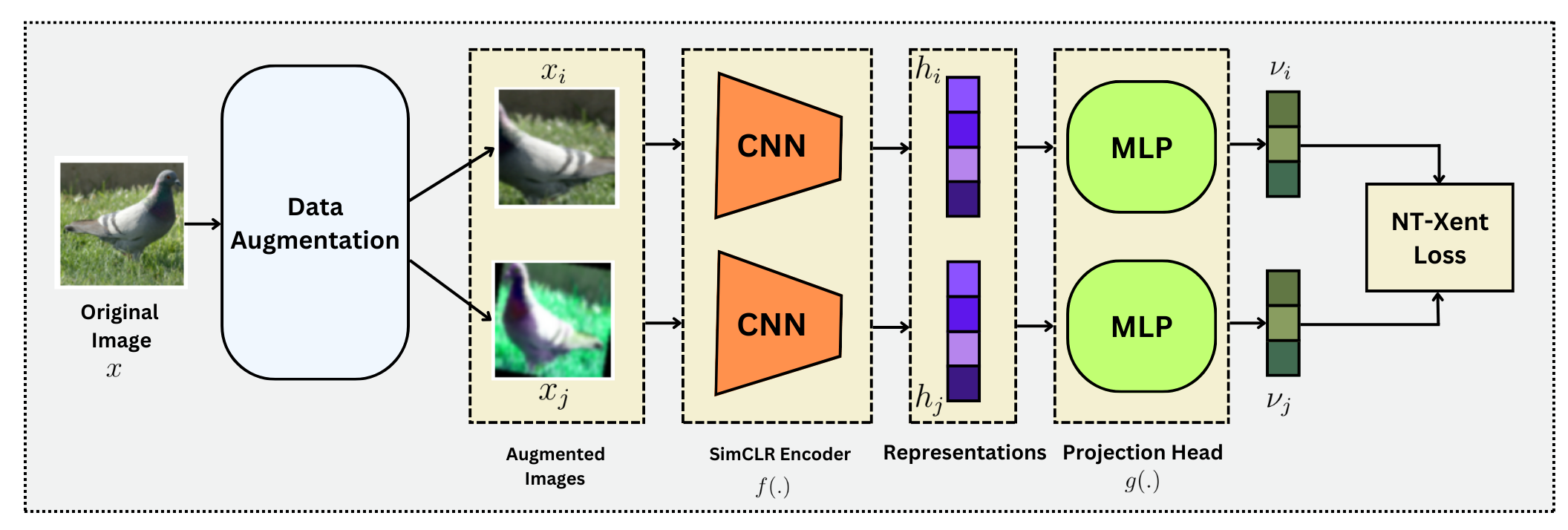
  Figure 1: SimCLR training framework at the buyer side

• The output of the backbone of the SimCLR model, denoted as $\mathbf{h}_{B}$, serves as the input to the encoder component of a variational auto-encoder which aims to minimize the deviation of the learned latent distribution from the standard normal prior distribution. The decoder also attempts to reconstruct these representations from sampled latent variables, $\mathbf{z}_{B}$. Subsequently, the buyer trains the VAE using its own datasets, as illustrated in Fig. 2. Here, The VAE provides a principled way to regularize the latent space by enforcing a Gaussian prior, ensuring that the latent space is well-structured.

  

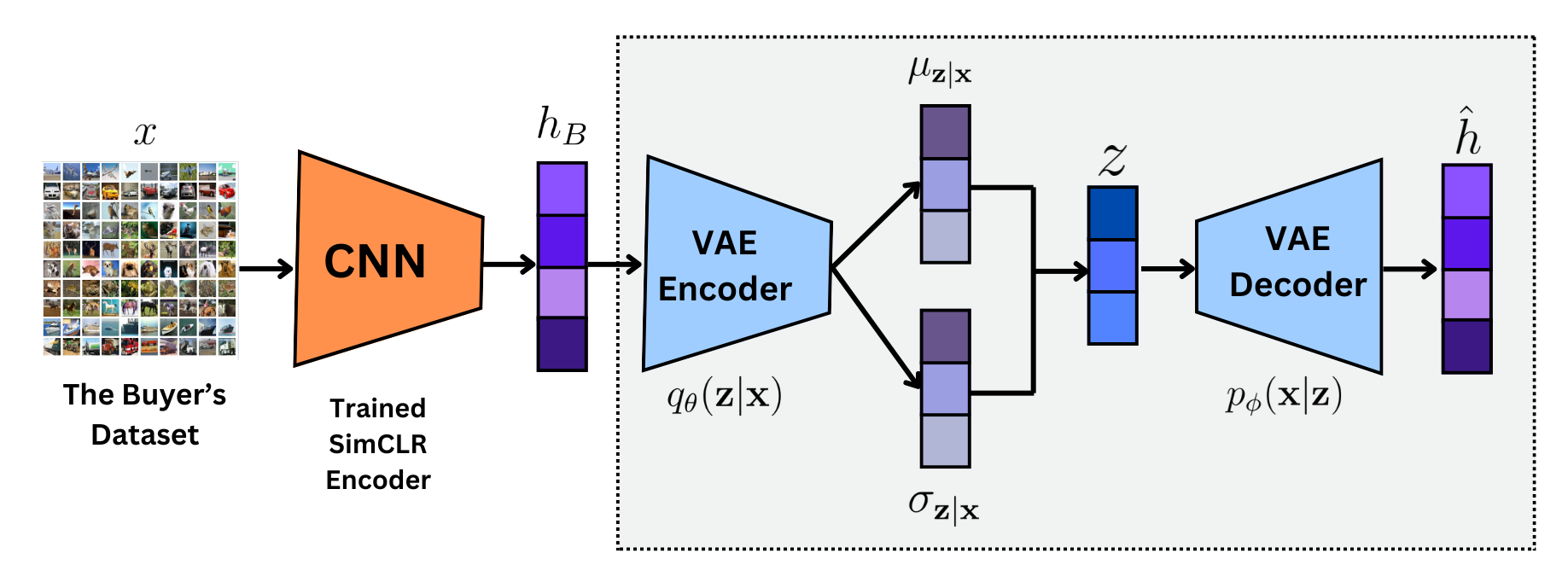
  Figure 2: VAE training at the buyer side

• The buyer shares its trained deep learning model, which represents the mapping function and consists of a concatenation of the SimCLR backbone and the VAE encoder, with the seller entities. Each seller, in turn, as depicted in Fig. 3 conducts an inference process utilizing the shared model with a random subset of their datasets to compute the corresponding latent variables as representations of its dataset, denoted as $\mathbf{Z}_{S_{i}}$ for seller-$i$.

• We assume that all entities within the data marketplace are honest, meaning no entity, especially the sellers, intends to deceive the buyer or use malicious behavior to influence a purchase. However, we also assume that each seller wants to keep their dataset, or its representations, private before any transactions. In this step, each seller is asked to send the mean and covariance of the representation of its dataset to the buyer. To make the representations private even after collecting the mean and covariance by the buyer, each seller adds Gaussian noise to the representations as differential privacy with Gaussian mechanism.

  Suppose the seller has $n$ representation vectors $\mathbf{z}_{j}\in\mathbb{R}^{d}$ (i.e., $\mathbf{Z}_{S_{i}}\in\mathbb{R}^{n\times d}$) where each vector $\mathbf{z}_{j}$ is bounded in terms of $\ell_{2}$-norm, i.e., $\left\lVert\mathbf{z}_{j}\right\rVert_{2}\leq R$. Then the $\ell_{2}$-sensitivity of mean function, $\mu=\frac{1}{n}\sum_{j=1}^{n}\mathbf{z}_{j}$, is bounded by $\Delta_{\mu}=\frac{2R}{n}$ which measures the maximum change in the mean when a single vector $\mathbf{z}_{i}$ is replaced by any other vector. Likewise, one can verify that the sensitivity of the covariance function $\Sigma=\frac{1}{n-1}\sum_{j=1}^{n}(\mathbf{z}_{j}-\mu)(\mathbf{z}_{j}-\mu)^{T}$ is bounded by $\Delta_{\Sigma}=\frac{4R^{2}}{n}+\frac{8R^{2}}{n^{2}}$ (see Appendix). For a certain $\epsilon,\delta\in(0,1)$, to achieve $(\epsilon,\delta)$-differential privacy in mean and covariance computation simultaneously, seller-$i$ should add random Gaussian noise $\mathbf{N}_{i}\sim\mathcal{N}(0,\sigma^{2}I)$ to its representation $\mathbf{Z}_{S_{i}}$, where $\sigma={\frac{\Delta_{\Sigma}}{\epsilon}\sqrt{2\ln{(1.25/\delta)}}}$. Therefore, seller-$i$ calculates the mean and covariance of its noisy data representations, denoted by $\mu_{S_{i}}$ and $\Sigma_{{S_{i}}}$ respectively.

• The sellers return the calculated statistics to the buyer for further calculations. Note that the subset of each seller’s dataset for inference is chosen uniformly at random from their dataset, and its size should be fixed for all sellers. In addition, the choice of $\epsilon$ and $\delta$ for the differential privacy depends on the desired balance between privacy and score of the data involved.

  

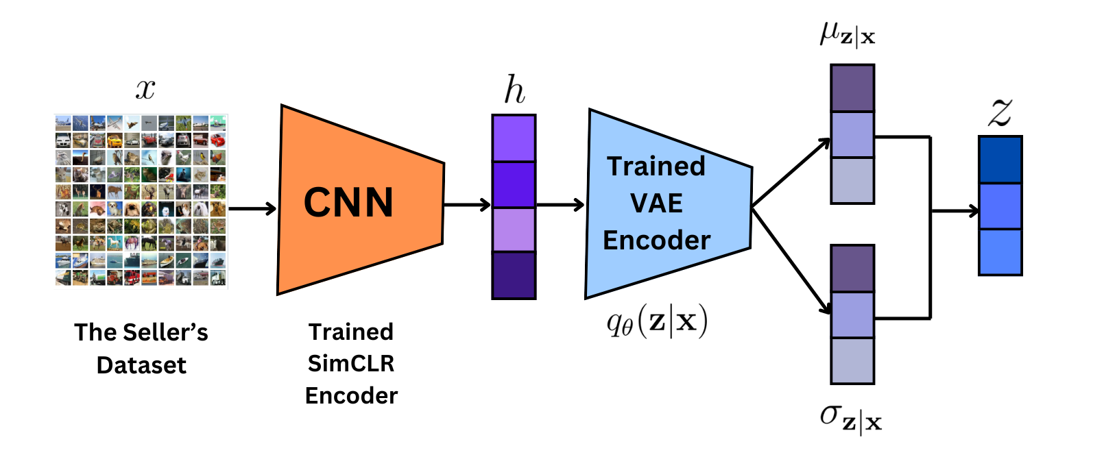
  Figure 3: Inference of the trained model at the seller side

• Since the distribution of the representations of all datasets, even after the addition of noise, is Gaussian, it becomes straightforward for the buyer to apply the Wasserstein distance metric to calculate the gain that each seller’s dataset might contribute. More precisely, for seller-$i$ the distance is calculated as

  $$W_{2}(\tilde{P}_{B},\tilde{P}_{S_{i}})=\big{(} \left\lVert\mu_{B}-\mu_{S_{i}}\right\rVert^{2}+\operatorname{tr}(\Sigma_{B})+\operatorname{tr}(\Sigma_{S_{i}})$$ (2)

  $$-2\operatorname{tr}\big{(}(\Sigma_{B}^{1/2}\Sigma_{S_{i}}\Sigma_{B}^{1/2})^{1/2}\big{)}\big{)}^{1/2},$$

  where $\mu_{B}$ and $\Sigma_{B}$ are the corresponding mean and covariance of the representations of the buyer’s dataset achieved by performing inference with the trained model. Additionally, $\tilde{P}_{B}$ and $\tilde{P}_{S_{i}}$ denote the distributions of the buyer’s and seller-$i$’s representations, respectively.

• After computing the mutual distances between the buyer’s dataset and each seller’s dataset, the buyer can make a decision based on the result. If the buyer selects the seller’s data with the greatest distance or dissimilarity, they can better cover the target population; if they select the dataset with the lower dissimilarity, they can enrich their existing dataset in the areas they already have data. Therefore, based on the calculated distance, the buyer can purchase data from the seller that best meets their needs.

The $\mathsf{PriArTa}$ method offers three significant advantages: it evaluates entire datasets instead of individual data points, which makes it computationally efficient even at large scales. It is also robust to common data transformations, ensuring that the assigned value of a dataset remains almost consistent even when modified (e.g., through resizing, cropping, or color adjustments). Additionally, $\mathsf{PriArTa}$ enables buyers to assess the value of datasets without direct access to raw data, protecting sellers’ privacy by allowing them to share only preprocessed and masked information.

5 Experiments and Results

In this section, we introduce the implementation details of $\mathsf{PriArTa}$, followed by the presentation of experimental results to demonstrate the performance of the proposed scheme. All experiments are simulated on a single machine using Intel(R) Core(TM) i9-7940X CPU @ 3.10GHz and NVIDIA Quadro P2000 with 5GB GDDR5 memory.

5.1 Implementation Details

Our experiments are conducted on the CIFAR-10 Krizhevsky (2009) and STL-10 Coates et al. (2011) datasets, which consists of 60,000 (32x32) and 13,000 (96x96) labeled color images across 10 classes, respectively. To simulate the buyer’s and sellers’ datasets with varying levels of similarity to the buyer’s data, we first split the dataset into several subsets according to predefined label distributions. In other words, the buyer and all sellers have subsets of the original datasets, CIFAR10 or STL10, each with a different distribution of classes, leading to imbalanced datasets.

Some of the subsets are then preprocessed using various transformations, such as random flipping, rotation, color jittering, and Gaussian blurring, to generate additional datasets for other sellers. However, these are not new datasets and will not provide additional learning information to the buyer after purchase, as they are merely augmented versions of the existing sellers’ or the buyer’s datasets.

To learn meaningful representations from the data, we employ the SimCLR self-supervised learning approach, as the proposed scheme. We utilize the ResNet-18He et al. (2016) as the backbone architecture and train a SimCLR model on the buyer’s dataset using the PyTorch Lightning framework Falcon & team (2019). The model is trained for 200/400 epochs with a batch size of 128/64, using the NTXentLoss as the contrastive loss function. The learned representations from the SimCLR model serve as the input to the subsequent VAE model. The VAE model consists of an encoder and a decoder network. The encoder takes the SimCLR representations as input and maps them to a latent space of dimension 64/32. The encoder network consists of fully connected layers with LeakyReLU activations and outputs the mean and log-variance of the latent distribution. The decoder network receives the sampled latent vector and reconstructs the original SimCLR representations through a series of fully connected layers.

The parameters of the backbone of the SimCLR is frozen and the VAE model is trained on the buyer’s data using the Adam optimizer. The loss function incorporates both the mean squared error (MSE) between the input and reconstructed representations, as well as the Kullback-Leibler (KL) divergence regularizer. After training, the combination of the SimCLR backbone and the VAE encoder is shared with other sellers for inference and computing the likelihood of their datasets. More precisely, each seller randomly selects a subset of their dataset of a certain size, then uses the shared model to compute the corresponding latent variables as representations of their datasets. To make the representation private, each seller employs differential privacy using the Gaussian mechanism with parameters $\epsilon=0.8$ and $\delta=10^{-5}$. Next, each seller returns the empirical mean and the covariance matrix of the noisy representations to the buyer, who computes the Wasserstein distance between the latent distributions of the buyer’s data and the sellers’ data using (2), i.e., the final valuation scores of each dataset.

For example, assume that the distributions of different classes in the buyer’s dataset and those of two other sellers are illustrated in Fig. 4. In this example, seller-2 has classes that are similar to those in the buyer’s dataset, whereas seller-1 covers additional classes, thereby offering greater diversity in the dataset available for purchase by the buyer.

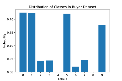
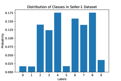
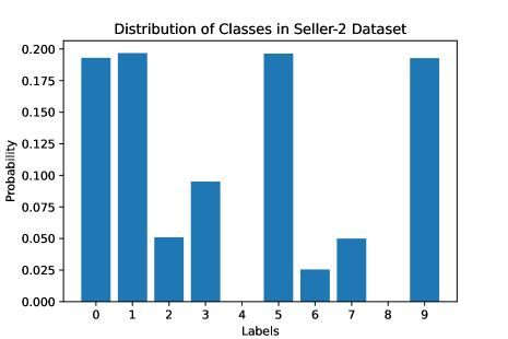
(a)	(b)	(c)

Figure 4: The probability distribution of datasets based on their respective classes. (a) represents the distribution of the buyer’s dataset, while (b) and (c) represent distributions for seller-1 and seller-2 respectively.

In addition, we consider five other sellers: seller-3 uses the dataset from seller-2 but applies multiple random transformations to images with varying probabilities. Seller-4 employs the buyer’s dataset with multiple random transformations applied at different probabilities. Seller-5 utilizes the buyer’s dataset with random flipping exclusively, while Seller-6 applies rotation alone to the same dataset. Lastly, Seller-7 applies only color jittering to the buyer’s dataset. Fig. 5 shows some sample images of the buyer’s dataset and four defined sellers’, where the underlying dataset is STL-10.

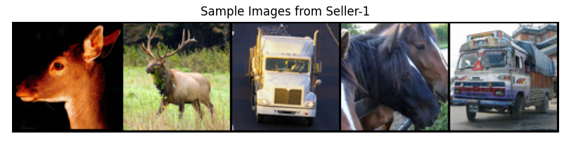
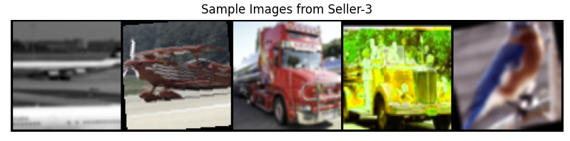
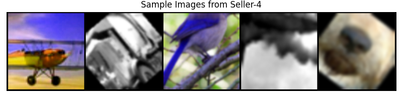
Figure 5: Sample images of the buyer’s dataset and four sellers’.

Fig. 6 shows the valuation scores of the aforementioned sellers’ datasets achieved by $\mathsf{PriArTa}$, where the underlying dataset are CIFAR-10 and STL-10. To emphasize the differences in the Wasserstein distances, we normalize these values. A common approach is to use Min-Max normalization, which scales the values to a fixed range, $[0,1]$. As shown in Fig. 6, if the buyer needs the most diverse dataset, the best option is the dataset from seller-1, as it provides the highest valuation score among all sellers.

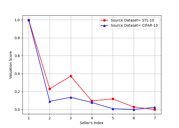
Figure 6: The valuation score of different sellers’ datasets, where the underlying datasets are CIFAR-10 and STL-10.

The overall goal of the buyer in purchasing data is to perform a task, which in this example, we assume to be classification. Initially, the buyer will train its model on the local dataset. After purchasing a new dataset, it will fine-tune the model. We assume that the VGG-16 network Simonyan & Zisserman (2014) is used for this classification task. Fig. 7 shows the model’s performance improvement in terms of test accuracy based on training on the buyer’s dataset and fine-tuning on other sellers’ datasets after 30 epochs. As shown, if the buyer purchases the dataset from seller-1, the accuracy improves the most, which is consistent with the results from the proposed method and the valuation scores.

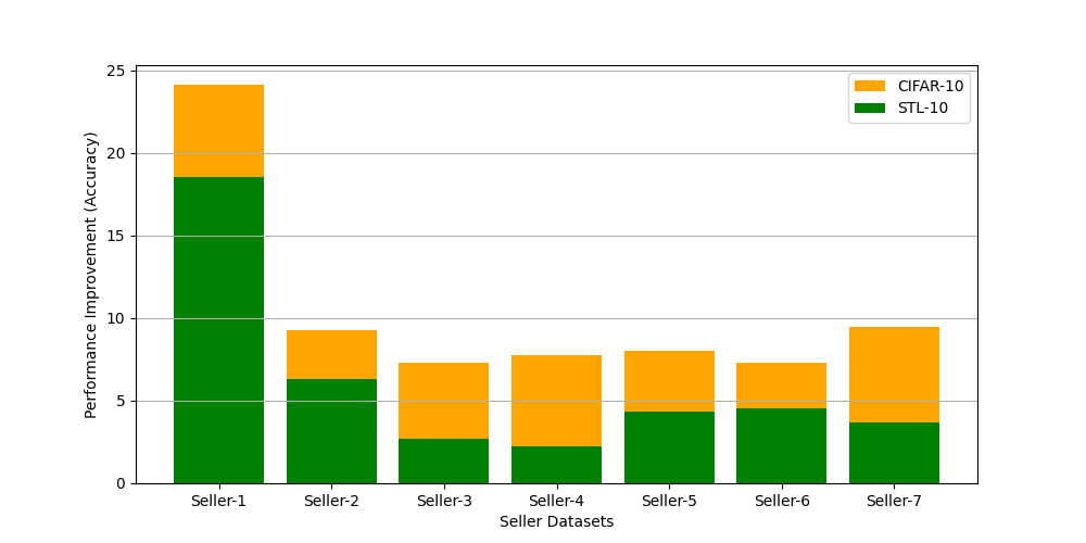
Figure 7: Performance improvement of the buyer’s model with seller datasets.

Note that the accuracy improvement from using sellers 4, 5, 6, and 7 is not due to the novelty or provision of new information. Instead, it is a result of the augmentation technique that the buyer can apply independently, without purchasing additional datasets from these sellers.

6 Conclusion

In this paper, we present $\mathsf{PriArTa}$, a novel approach for privacy-preserving and augmentation-robust data valuation in data marketplaces. $\mathsf{PriArTa}$ is a task-agnostic method that enables buyers to evaluate the whole dataset of each seller without full access, ensuring privacy and minimizing redundancy in the purchase. Experimental results on real-world image datasets demonstrate the effectiveness of $\mathsf{PriArTa}$ in providing reliable data valuation, even in the presence of sellers who have augmented versions of each other’s datasets.

Appendix A Sensitivity of Mean and Covariance Functions

Suppose we have $n$ vectors $\mathbf{x}_{i}\in\mathbb{R}^{d}$, where each vector has a bounded $\ell_{2}$-norm such that $\left\lVert\mathbf{x}_{i}\right\rVert_{2}\leq R$. We define function $\mu$ that computes the mean of these vectors as $\mu=\frac{1}{n}\sum_{i=1}^{n}\mathbf{x}_{i}$. To determine the $\ell_{2}$-sensitivity of the mean function, we need to consider the effect of changing one vector $\mathbf{x}^{\prime}_{j}$ among all vectors. When a single vector is changed, the maximum change in the mean is bounded as

$$\left\lVert\mu^{\prime}-\mu\right\rVert_{2}=\left\lVert\frac{1}{n}(\mathbf{x}^{\prime}_{j}-\mathbf{x}_{j})\right\rVert_{2}\leq\frac{2R}{n},$$ (3)

where $\mu^{\prime}$ is the mean vector after the change, and the last inequality holds because of the assumption that all vectors are bounded within a sphere of radius $R$.

To calculate the change in the covariance $\Sigma=\frac{1}{n-1}\sum_{i=1}^{n}(\mathbf{x}_{i}-\mu)(\mathbf{x}_{i}-\mu)^{T}$ due to the change in a single vector, we should consider the worst case change which occurs when we replace a vector that was $R$ away from the mean in one direction with a vector that is $R$ away from the mean in the opposite direction. Let us denote the original vector by $\mathbf{x}_{j}=\mu+R\mathbf{u}$ and the replaced one by $\mathbf{x}^{\prime}_{j}=\mu-R\mathbf{u}$, where $\mathbf{u}$ is a unit vector in some direction. The changes in the covariance matrix when we replace $\mathbf{x}_{j}$ with $\mathbf{x}^{\prime}_{j}$ is

$$\Delta\Sigma=\frac{1}{n-1}\bigg{(}(\mathbf{x}^{\prime}_{j}-\mu^{\prime})(\mathbf{x}^{\prime}_{j}-\mu^{\prime})^{T}-(\mathbf{x}_{j}-\mu)(\mathbf{x}_{j}-\mu)^{T}$$

$$+\sum_{i=1,i\neq j}^{n}\big{(}(\mathbf{x}_{i}-\mu^{\prime})(\mathbf{x}_{i}-\mu^{\prime})^{T}-(\mathbf{x}_{i}-\mu)(\mathbf{x}_{i}-\mu)^{T}\big{)}\bigg{)},$$

where $\mu^{\prime}$ is the new mean after replacing $\mathbf{x}_{j}$ with $\mathbf{x}^{\prime}_{j}$ and we have $\mu^{\prime}=\mu+(\mathbf{x}^{\prime}_{j}-\mathbf{x}_{j})/n=\mu-2R\mathbf{u}/n$. In addition, we have

$$\mathbf{x}^{\prime}_{j}-\mu^{\prime}=(\mathbf{x}^{\prime}_{j}-\mu)+(\mu-\mu^{\prime})=-R\mathbf{u}+2R\mathbf{u}/n.$$

Substituting these back into the $\Delta\Sigma$

$$\Delta\Sigma= \frac{1}{n-1}\bigg{(}R^{2}\mathbf{u}\mathbf{u}^{T}(1-\frac{2}{n})^{2}-R^{2}\mathbf{u}\mathbf{u}^{T}$$

$$+\sum_{i=1,i\neq j}^{n}\big{(}\frac{2R}{n}((\mathbf{x}_{i}-\mu)\mathbf{u}^{T}+\mathbf{u}(\mathbf{x}_{i}-\mu)^{T})+\frac{4R^{2}}{n^{2}}\mathbf{u}\mathbf{u}^{T}\big{)}\bigg{)}.$$

Using triangle inequality properties of the Frobenius norm we have

$$\left\lVert\Delta\Sigma\right\rVert_{F}\leq \frac{1}{n-1}\bigg{(}\frac{4R^{2}}{n}|(\frac{1}{n}-1)|\left\lVert\mathbf{u}\mathbf{u}^{T}\right\rVert_{F}$$

$$+\sum_{i=1,i\neq j}^{n}\big{(}\frac{4R}{n}\left\lVert(\mathbf{x}_{i}-\mu)\mathbf{u}^{T}\right\rVert_{F}+\frac{4R^{2}}{n^{2}}\left\lVert\mathbf{u}\mathbf{u}^{T}\right\rVert_{F}\big{)}\bigg{)}$$

$$\leq\frac{4R^{2}}{n}+\frac{8R^{2}}{n^{2}}.$$

References

- Agarwal et al. (2019) Agarwal, A., Dahleh, M., and Sarkar, T. A marketplace for data: An algorithmic solution. In Proceedings of the 2019 ACM Conference on Economics and Computation, pp. 701–726, 2019.
- Amiri et al. (2023) Amiri, M. M., Berdoz, F., and Raskar, R. Fundamentals of task-agnostic data valuation. In Proceedings of the AAAI Conference on Artificial Intelligence, volume 37, pp. 9226–9234, 2023.
- Bachman et al. (2019) Bachman, P., Hjelm, R. D., and Buchwalter, W. Learning representations by maximizing mutual information across views. Advances in neural information processing systems, 32, 2019.
- Chen et al. (2020) Chen, T., Kornblith, S., Norouzi, M., and Hinton, G. A simple framework for contrastive learning of visual representations. In International conference on machine learning, pp. 1597–1607. PMLR, 2020.
- Chen et al. (2016) Chen, X., Kingma, D. P., Salimans, T., Duan, Y., Dhariwal, P., Schulman, J., Sutskever, I., and Abbeel, P. Variational lossy autoencoder. arXiv preprint arXiv:1611.02731, 2016.
- Coates et al. (2011) Coates, A., Ng, A. Y., and Lee, H. An analysis of single-layer networks in unsupervised feature learning. In Proceedings of the Fourteenth International Conference on Artificial Intelligence and Statistics, pp. 215–223. JMLR Workshop and Conference Proceedings, 2011.
- Cook (1977) Cook, R. D. Detection of influential observation in linear regression. Technometrics, 19(1):15–18, 1977.
- Dwork et al. (2006) Dwork, C., McSherry, F., Nissim, K., and Smith, A. Calibrating noise to sensitivity in private data analysis. In Theory of Cryptography: Third Theory of Cryptography Conference, TCC 2006, New York, NY, USA, March 4-7, 2006. Proceedings 3, pp. 265–284. Springer, 2006.
- Dwork et al. (2014) Dwork, C., Roth, A., et al. The algorithmic foundations of differential privacy. Foundations and Trends® in Theoretical Computer Science, 9(3–4):211–407, 2014.
- Falcon & team (2019) Falcon, P. and team, T. P. L. PyTorch Lightning: Light research and production code for deep learning. https://github.com/PyTorchLightning/pytorch-lightning, 2019. Accessed: 2024-07-03.
- Ghorbani & Zou (2019) Ghorbani, A. and Zou, J. Data shapley: Equitable valuation of data for machine learning. In International conference on machine learning, pp. 2242–2251. PMLR, 2019.
- Ghorbani et al. (2020) Ghorbani, A., Kim, M., and Zou, J. A distributional framework for data valuation. In International Conference on Machine Learning, pp. 3535–3544. PMLR, 2020.
- Gibbs & Su (2002) Gibbs, A. L. and Su, F. E. On choosing and bounding probability metrics. International statistical review, 70(3):419–435, 2002.
- Gretton et al. (2012) Gretton, A., Borgwardt, K. M., Rasch, M. J., Schölkopf, B., and Smola, A. A kernel two-sample test. The Journal of Machine Learning Research, 13(1):723–773, 2012.
- He et al. (2016) He, K., Zhang, X., Ren, S., and Sun, J. Deep residual learning for image recognition. In Proceedings of the IEEE Conference on Computer Vision and Pattern Recognition, pp. 770–778, 2016.
- Jacot et al. (2018) Jacot, A., Gabriel, F., and Hongler, C. Neural tangent kernel: Convergence and generalization in neural networks. Advances in neural information processing systems, 31, 2018.
- Jia et al. (2019) Jia, R., Dao, D., Wang, B., Hubis, F. A., Gurel, N. M., Li, B., Zhang, C., Spanos, C. J., and Song, D. Efficient task-specific data valuation for nearest neighbor algorithms. arXiv preprint arXiv:1908.08619, 2019.
- Just et al. (2023) Just, H. A., Kang, F., Wang, J. T., Zeng, Y., Ko, M., Jin, M., and Jia, R. Lava: Data valuation without pre-specified learning algorithms. arXiv preprint arXiv:2305.00054, 2023.
- Kantorovich (1942) Kantorovich, L. V. On the translocation of masses. In Dokl. Akad. Nauk. USSR (NS), volume 37, pp. 199–201, 1942.
- Kasiviswanathan et al. (2011) Kasiviswanathan, S. P., Lee, H. K., Nissim, K., Raskhodnikova, S., and Smith, A. What can we learn privately? SIAM Journal on Computing, 40(3):793–826, 2011.
- Kingma & Welling (2013) Kingma, D. P. and Welling, M. Auto-encoding variational bayes. CoRR, abs/1312.6114, 2013.
- Krizhevsky (2009) Krizhevsky, A. Learning multiple layers of features from tiny images. Master’s thesis, University of Toronto, Dept. of Computer Science, 2009.
- Kullback & Leibler (1951) Kullback, S. and Leibler, R. A. On information and sufficiency. The annals of mathematical statistics, 22(1):79–86, 1951.
- Kwon & Zou (2021) Kwon, Y. and Zou, J. Y. Beta shapley: a unified and noise-reduced data valuation framework for machine learning. In International Conference on Artificial Intelligence and Statistics, 2021.
- Lu et al. (2024) Lu, C., Amiri, M. M., and Raskar, R. Private data measurements for decentralized data markets. In ICLR 2024 Workshop on Data-centric Machine Learning Research (DMLR): Harnessing Momentum for Science, 2024.
- Nohyun et al. (2022) Nohyun, K., Choi, H., and Chung, H. W. Data valuation without training of a model. In The Eleventh International Conference on Learning Representations, 2022.
- Peyré et al. (2019) Peyré, G., Cuturi, M., et al. Computational optimal transport: With applications to data science. Foundations and Trends® in Machine Learning, 11(5-6):355–607, 2019.
- Rumelhart et al. (1986) Rumelhart, D. E., Hinton, G. E., and Williams, R. J. Learning representations by back-propagating errors. nature, 323(6088):533–536, 1986.
- Shapley (1953) Shapley, L. S. A value for n-person games. In Contributions to the Theory of Games, volume 2 of Annals of Mathematics Studies, pp. 307–317. Princeton University Press, Princeton, NJ, 1953.
- Simonyan & Zisserman (2014) Simonyan, K. and Zisserman, A. Very deep convolutional networks for large-scale image recognition. CoRR, abs/1409.1556, 2014.
- Sun et al. (2017) Sun, C., Shrivastava, A., Singh, S., and Gupta, A. Revisiting unreasonable effectiveness of data in deep learning era. In Proceedings of the IEEE international conference on computer vision, pp. 843–852, 2017.
- Tay et al. (2022) Tay, S. S., Xu, X., Foo, C. S., and Low, B. K. H. Incentivizing collaboration in machine learning via synthetic data rewards. In Proceedings of the AAAI Conference on Artificial Intelligence, volume 36, pp. 9448–9456, 2022.
- Wang & Jia (2023) Wang, J. T. and Jia, R. Data banzhaf: A robust data valuation framework for machine learning. In International Conference on Artificial Intelligence and Statistics, pp. 6388–6421. PMLR, 2023.
- Wu et al. (2022) Wu, Z., Shu, Y., and Low, B. K. H. Davinz: Data valuation using deep neural networks at initialization. In International Conference on Machine Learning, pp. 24150–24176. PMLR, 2022.