Measurement Schemes for Quantum Linear Equation Solvers

Abstract

Solving Computational Fluid Dynamics (CFD) problems requires the inversion of a linear system of equations, which can be done using a quantum algorithm for matrix inversion [1]. However, the number of shots required to measure the output of the system can be prohibitive and remove any advantage obtained by quantum computing. In this work we propose a scheme for measuring the output of QSVT matrix inversion algorithms specifically for the CFD use case. We use a Quantum Signal Processing (QSP) based amplitude estimation algorithm [2] and show how it can be combined with the QSVT matrix inversion algorithm. We perform a detailed resource estimation of the amount of computational resources required for a single iteration of amplitude estimation, and compare the costs of amplitude estimation with the cost of not doing amplitude estimation and measuring the whole wavefunction. We also propose a measurement scheme to reduce the number of amplitudes measured in the CFD example by focussing on large amplitudes only. We simulate the whole CFD loop, finding that thus measuring only a small number of the total amplitudes in the output vector still results in an acceptable level of overall error.

I Introduction

Solving systems of linear equations is one of the promising applications of quantum computers outside of chemistry simulations and the hidden subgroup problem for factoring [3]. In this paper we focus upon the measurement problem for a Quantum Linear Equations System (QLES) algorithm [4] based upon the Quantum Singular Value Transform (QSVT) [1]. This algorithm uses matrix inversion to solve for $\mathbf{x}$ the equation

$$A\mathbf{x}=\mathbf{b},$$ (1)

by inverting the matrix $A$ and applying it to the input vector, $\mathbf{b}$. At the completion of the algorithm all the qubits are measured and we post select upon a subset (the flag qubits) being measured all in the $\ket{0}$ state. The probability of this outcome is affected by the subnormalisation, $\kappa$ of the matrix to be inverted, and can be quite small which requires many repeats of the circuit to measure the output. Using an amplitude amplification algorithm is a common method of projecting onto the $\ket{0}^{\otimes_{\textrm{flag}}}$ state, and in this report we will detail a scheme that uses amplitude estimation to also project onto individual basis vectors representing elements of the corrections vector. We will also use an amplitude estimation algorithm that is based on Quantum Signal Processing (QSP), similar to QSVT [2].

The QLES algorithm essentially uses a quantum algorithm (here QSVT) as a drop-in subroutine for the inversion of a matrix and return of a corrections vector. The quantum computer solves the linear part of the problem, and we use existing classical methods to linearise the non-linear equations and apply returned corrections. We are concerned here with measurement of the quantum state that describes this vector, which in the naive case requires $\frac{1}{\epsilon^{2}}$ measurements of the (post-selected) output qubits. In the QLES algorithm $\mathbf{x}$ is a vector of corrections that we apply to the input vector in an iterative procedure until the system has converged. We can use the nature of the corrections vector to make some simplifying assumptions. Figure 1(a) shows an example output for a corrections vector from the beginning of a program, and 1(b) shows one from the final iteration. We see that large peaks in the amplitude are present at the beginning of the iteration, with a small number of larger peaks still being the dominant feature towards the end of the algorithm. Using this feature we suggest that a measurement scheme based upon amplitude encoding is useful, where we estimate the amplitude of the largest peaks and return this as an approximate correction. As the corrections in Figure 1 also contain negative corrections, we must use a measurement scheme which is sensitive to the sign of the amplitude.

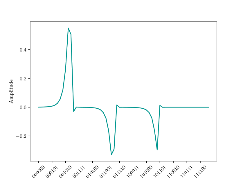
(a)

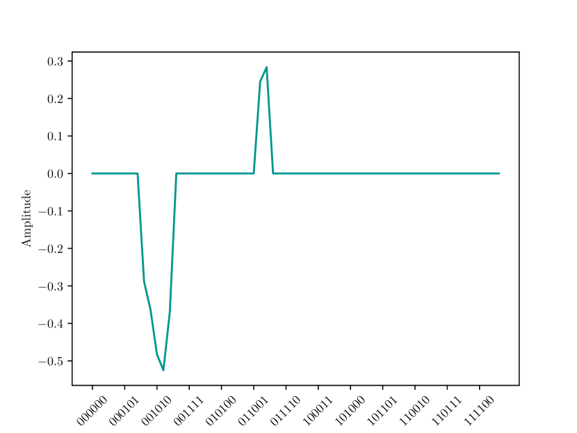
(b)

Figure 1: Normalised output vectors of the QLES algorithm, these will be stored as probability amplitudes of the output qubits.  1(a): A vector from early in the iteration,  1(b): A vector from late in the iteration.

We denote the state at the end of the matrix inversion algorithm as $\ket{\psi}$, and the algorithm itself as implemented by the unitary $U_{\psi}$; this allows us to quantify the resources required to output a correction vector in the terms of oracle access to the circuit implementing $U_{\psi}\ket{0^{\otimes n}}=\ket{\psi}$. The naive approach to finding the corrections vector is to use quantum state tomography to accurately record the amplitude of each basis vector ($\ket{00\dots 0},\ket{00\dots 1}\dots$), which requires exponential calls to $U_{\psi}$ in the number of qubits, $n$ [5]. Advancements have been made in quantum state tomography, including maximum likelihood estimation (MLE) [6, 5], neural network based methods [7], and tensor network based methods [8]. If the state being measured can be represented as a Matrix Product State, MPS, measurement time is linear in $n$ [8], neural network methods can be used to accurately reconstruct observables of the quantum state [7], but no guarantees on the number of shots required are given. Alternatively, the quantum signal processing approach to Amplitude Estimation discussed in [2] requires a number of calls to the oracle that scales with the length of the polynomial used to construct the reflection operator.

In this paper we will present a measurement scheme using amplitude estimation from QSP. We are considering the problem from a CFD perspective, which we will introduce in Section II. The quantum algorithm combines ideas from [2] which shows how to do amplitude estimation using QSP and [9] which discusses embedding a QSVT algorithm within a QSP protocol. As the corrections vectors have a defined sign, we will use the real amplitude estimation scheme from [10] to provide and estimate of the sign of the amplitude. The combination of these three algorithms is discussed in Section III. In Section IV we discuss the measurement scheme specifically for corrections vectors, where we propose reducing the number of amplitudes to measure, focussing on the peaks only. In Section V we perform a resource estimation of measuring a single amplitude of the correction vector using amplitude estimation, and compare that cost to not running the amplitude estimation algorithm and receiving an estimator of all amplitudes, we also simulate the scheme discussed in Section IV within a classical CFD loop, comparing the performance of an algorithm with a high cut-off to that with a low cut-off (the threshold determining which amplitudes are considered). Finally, in Section VI we will conclude and discuss the results.

II CFD Method

Computational Fluid Dynamics (CFD) is used to simulate and engineer many modern components that interact with fluids, e.g. the flow of gas through a turbine engine [11]. The Navier-Stokes equations describe the conservation of mass, momentum, and energy within the flow of a fluid. The equations are highly non-linear, however, many CFD solvers adopt an iterative approach whereby the equations are linearised and then solved to provide an update to the non-linear flow field. Each linearised system can be expressed in the form of residual equations:

$$A^{n}\mathbf{\delta x^{n+1}} =\mathbf{\delta b^{n}}=\mathbf{b^{n}}-A^{n}\mathbf{x^{n}}$$ (2)

$$\mathbf{x^{n+1}} =\mathbf{x^{n}}+\mathbf{\delta x^{n+1}}$$

where $A^{n}$ and $\mathbf{b^{n}}$ depend on $\mathbf{x^{n}}$ and the iterations begin with a initial guess for the flow field at $n=0$. The iterations are repeated until the $L_{2}$ norm of the non-linear equation errors, $||\mathbf{\delta b^{n}}||$, falls below a specified threshold, $\epsilon_{\textrm{tol}}$. In the work here, we will use $\epsilon_{\textrm{tol}}=1\times 10^{-9}$. Note that to use a QLES the state vectors $\mathbf{\delta x}$ and $\mathbf{\delta b}$ must be normalised. This is why the vectors in Figures 1(a) and  1(b) do not show the reduction in the $L_{2}$ residual error.

In this work, we use two different solvers, either the Semi-Implicit Method for Pressure Linked Equations (SIMPLE) solver, a derivation of which can be found in the Appendix of Ref. [4], or a coupled solver. In the former, the linearised momentum and mass conservation equations are solved separately, leading to a Poisson type equation for corrections to the pressure field. In the latter, the linearised equations are combined in a single, coupled, matrix system [12]. This has the benefit of providing faster convergence. In this work we solve the CFD problem for a 1D convergent-divergent channel, sometimes referred to as a nozzle, and the discretisation scheme used is also described in [4]. We can consider two types of fluid, incompressible and compressible: for the former the density is constant, whereas, for the latter the Perfect Gas Law and energy conservation are used to relate pressure, density and temperature.

III Amplitude Estimation for Corrections Vectors

In this section we will introduce the three algorithms we combine to measure the output vector of a matrix inversion problem using QSVT. Firstly, we will review the algorithm of Rall et. al [2] where they show how to implement amplitude estimation using QSP, achieving a constant factor improvement and providing an estimate of query complexity to $Q_{\Pi}$, or the number of iterations of the amplitude estimation circuit. As we are using a QSVT circuit to implement matrix inversion we need to show that the QSP protocol interacts with the matrix inversion algorithm correctly. Secondly, we use the results of [9] to do this, using the fact that the polynomial approximating $f(A)\approx A^{-1}$ is real, and therefore an anit-symmetric list of phase factors can be generated. Thirdly, as the amplitude estimatino scheme as described so far can only estimate $|a|$ instead of $a$, we use the real amplitude estimation scheme of [10] to modify our scheme to give the sign of $a$ also. Finally, we combine the three algorithms discussed to give an overall query complexity for a single amplitude.

In [2] an amplitude estimation technique is developed that instead of using oracle access to reflections $Z_{\Pi},Z_{\psi}$ about axes defined by a projector and a state, $\ket{\Pi},\ket{\psi}$, assumes access to rotations around those axes, $e^{i\phi Z_{\Pi}},e^{i\phi Z_{\psi}}$. Access to the rotation operators allows us to use techniques from Quantum Signal Processing (QSP) [13] for a constant factor improvement in the number of oracle calls, and to use other useful techniques such as non-destructive amplitude estimation, where we return a copy of $\ket{\psi}$ at the end of the algorithm. QSP techniques allow us to choose the rotation values $\phi$ such that we can implement a polynomial of the amplitude, $P(a)$.

III.1 Vanilla Amplitude Estimation

Amplitude estimation was first developed in Ref. [14], building upon a subroutine of Grover’s algorithm [15] and Quantum Phase Estimation [16]. In all amplitude estimation routines, we begin with the state we wish to investigate, $\ket{\psi}$, and a projector, $\Pi$, onto the subspace we wish to measure the amplitude, $a$, of, $a=|\Pi\ket{\psi}|$. The projector and its complement can be turned into basis vectors of a two-dimensional Hilbert space:

$$\ket{\Pi} =a^{-1}\Pi\ket{\psi}$$ (3)

$$\ket{\Pi^{\perp}} =\bar{a}^{-1}(I-\Pi)\ket{\psi}$$

where $a$ is the amplitude of the state we wish to measure, and $\bar{a}=\sqrt{1-a^{2}}$. We can express $\ket{\psi}$ in terms of this new orthonormal basis:

$$\ket{\psi}=a\ket{\Pi}+\bar{a}\ket{\Pi^{\perp}},$$ (4)

and define another basis vector to complement $\ket{\psi}$:

$$\ket{\psi^{\perp}}=\bar{a}\ket{\Pi}-a\ket{\Pi^{\perp}}.$$ (5)

We use these two orthonormal bases to define the reflection operators,

$$Z_{\psi} =\ket{\psi}\bra{\psi}-\ket{\psi^{\perp}}\bra{\psi^{\perp}}$$ (6)

$$Z_{\Pi} =\ket{\Pi}\bra{\Pi}-\ket{\Pi^{\perp}}\bra{\Pi^{\perp}}$$

which reflect the state around the projection and $\psi$ axes, resulting in a rotation. Implementing this rotation (the Grover operator) is the basis of Grover’s algorithm for search [15], and applying quantum phase estimation to the Grover operator was the first implementation of an amplitude estimation algorithm [14]. In 2019 multiple Ref.s [17, 18, 19] introduced methods of removing the Quantum Fourier Transform from the amplitude estimation algorithm, keeping the same query complexity. Ref. [17] gave a proof for the lower bound query complexity, in [18] multiple samples of the Grover operator are taken, and Maximum Likelihood Estimation (MLE) is used to estimate the amplitude which improves the constant factor in query complexity, but has no proof. In Ref. [19] the QFT of the original amplitude estimation algorithm is replaced with Hadamard tests, in a similar manner to the replacement of QFT with Hadamard tests in the Iterative Quantum Phase Estimation algorithm [20]. Ref. [21] is another iterative amplitude estimation algorithm that improves on the constant factors of [19], and has a rigorous proof. Ref. [22] improves on MLE amplitude estimation [18] by showing a way to avoid values of the amplitude where MLEAE fails, and gives a method of achieving amplitude estimation with a given circuit depth, which is useful in early fault tolerant quantum computers, where the number of qubits and noise level restricts the overall circuit depth.

III.2 Amplitude Estimation from Quantum Signal Processing

The scheme of [2] which we will use to implement amplitude estimation on a QLES correction vector requires access to arbitrary rotations around the reflection axes, $e^{i\phi_{0}Z_{\psi}},e^{i\phi_{1}Z_{\Pi}}$. Choice of phase factors, $\phi$, allows us to implement a family of polynomials on the amplitude, $P(a)$, which we can sample from with multiple shots of the circuit to get an estimator $|P(a)|^{2}$. This sets up a quantum signal processing problem, where we are sampling from the polynomial $P$, where we measure in the $\{\ket{\psi},\ket{\psi^{\perp}}\},(\{\ket{\Pi},\ket{\Pi^{\perp}}\})$ basis and return the state $\ket{\psi}(\ket{\Pi})$ with probability $|P(a)|^{2}$, allowing us to sample from an estimator of $a$. Each coin toss requires a number of oracle queries that depends on the degree of the polynomial, $O(\textrm{deg}(P))$. In Ref. [2] an algorithm that samples from Chebyshev polynomials is introduced, ChebAE, which has the lowest query complexity, due to the fact that Chebyshev polynomials have the greatest variation over the range $a\in[0,1]$.

We have chosen a QSP algorithm as the basis of our amplitude estimation routine, yet as we have also used a QSVT implementation of the matrix inversion algorithm we must show that we are able to compose the two circuits together without incurring significant errors. Thankfully there has been recent work [23, 9, 24] we can use to show that the composition of the two functions for matrix inversion and amplitude amplification can be achieved when both are expressed as QSVT algorithms. We will use the definitions from [9] of an embeddable QSVT algorithm.

We require the matrix inversion subroutine to be an embeddable QSVT algorithm. An embeddable algorithm allows us to nest the first algorithm as the signal operator of the outer algorithm, in general this is not possible for reasons we will briefly explain here, for a fuller review see Ref. [9]. A QSVT algorithm is the lifted version of a QSP algorithm, where we act upon some 2 dimensional subspace of a multi-qubit Hilbert space, and we act upon the singular values of block-encoded matrices, instead of acting on the Hilbert space of a single qubit applying functions to a scalar value in QSP. The 2 dimensional subspace of the QSVT algorithm is then described by the projectors $\Pi_{\textrm{inv}},\tilde{\Pi}_{\textrm{inv}}$, and the QSVT algorithm can be described as the circuit implementing,

$$U_{\Phi_{0}}=e^{i\phi_{1}^{0}(2\tilde{\Pi}_{\textrm{inv}}-I)}U_{0}\prod_{j=1}^{(n-1)/2}\left[e^{i\phi_{2j-1}(2\Pi_{\textrm{inv}}-I)}U_{0}^{\dagger}e^{i\phi_{2j}(2\tilde{\Pi}_{\textrm{inv}}-I)}U_{0}\right]$$ (7)

for even $n$ the number of phase factors in the inversion protocol, $\phi^{0}_{j}$. Where $U_{0}$ implements the block encoding of the matrix to be inverted.

In the definition of nested QSVT protocols Ref. [9] makes the distinction between flatly nested and deeply nested QSVT protocols, where a flatly nested protocol shares its projectors with the outer QSVT routine. As we are nesting a matrix inversion algorithm within an amplitude estimation algorithm, we necessarily have different projectors so will focus upon deeply nested QSVT protocols.

To nest a QSVT protocol we replace the projectors of that protocol with a transformed projector, defined by the unitary transformation of the outer QSVT protocol, $U_{\Phi_{1}}$:

$$\tilde{\Pi}\rightarrow U_{\Phi_{1}}\tilde{\Pi}U^{\dagger}_{\Phi_{1}}.$$ (8)

It is possible to choose any projector, $\Pi$, for the amplitude estimation algorithm, but the use of QSVT in the matrix inversion step indicates that we should project onto a tensor product of the all-$\ket{0}$ state of the flag qubits (which ensures we are in the top-left block of the block encoding), and some basis state corresponding to a location of a chosen correction peak.

The phase factors of the outer protocol are also restricted to be antisymmetric. A list of phase factors is antisymmetric when it remains the same under reversal and negation, i.e. for a list of phase factors of length $2d$ the phase factors are $\mathbf{\Phi}_{1}=\left\{\phi_{0},\phi_{1},\phi_{2}\dots,\phi_{d},-\phi_{d},\dots,-\phi_{2},-\phi_{1},-\phi_{0}\right\}$, and for an odd polynomial the central phase factor must be 0: $\mathbf{\Phi}_{1}=\left\{\phi_{0},\phi_{1},\phi_{2}\dots,\phi_{d},0,-\phi_{d},\dots,-\phi_{2},-\phi_{1},-\phi_{0}\right\}$. This restriction on the phase factors requires that the outer polynomial is real, and is unique for that polynomial. The polynomial is therefore a rotation on the $XY$ plane of the Bloch sphere for all $x$, and anticommutes with the $Z$ rotations of the outer protocol. If the polynomial were not real there would be a rotation that commutes with the $Z$ rotations of the inner protocol, and the composition of the function then loses information about this part of the inner function. This argument is a brief explanation of the one in [9, Corollary II.4.1], which can be referenced for a full explanation. In the follow-up work, Ref. [24] the authors discuss extensions to a greater family of protocols.

For our purposes all that remains is to show that the outer protocol, that discussed in [2], implements a real polynomial and therefore that an antisymmetric list of phase factors exists. Thankfully, the algorithm we will be using from Ref. [2] is ChebAE which implements amplitude estimation using Chebyshev polynomials as the $P(a)$ transformation, and as the Chebyshev polynomials are real we can guarantee that an antisymmetric list of phase factors exist, and therefore that we can embed the matrix inversion QSVT protocol into the ChebAE protocol.

III.3 Resource Estimation of the ChebAE algorithm

Ref. [2] provides an average query complexity to the oracles that implement rotations in the ChebAE algorithm, but for a full resource estimation we need to determine the cost of a single oracle in our matrix inversion setting. Instead of the reflection operators, $Z_{\psi},Z_{\Pi}$ in Equation 6 we require access to the rotations about the axis defined by these reflections, $e^{i\phi_{j}Z_{\psi}},e^{i\phi_{j}\Pi}$. Following the exposition in [2], we can implement $Z_{0^{n}}=2\ket{0^{n}}\bra{0^{n}}-I$ with Toffoli gates and a $Z$ gate, and therefore $e^{i\phi_{j}Z_{0^{n}}}$ with the same number of Toffoli gates and a $Z$ rotation. Implementation of $e^{i\phi_{j}Z_{\psi}}$ is then done via $U_{\psi}e^{i\phi_{j}Z_{0^{n}}}U^{\dagger}_{\psi}$. For the rotation $e^{i\phi_{j}Z_{\Pi}}$ we make a similar argument, that instead of trying to implement $Z_{0^{n}}$, $Z_{\Pi}$ is a projection onto some other, known, basis state. This projector has an exact cost that differs for the exact basis state considered, but is generally $\mathcal{O}(n)$ Toffoli gates. The rotation can be implemented by replacing the final $Z$ gate with a $R_{z}$ gate. Therefore $e^{i\phi_{j}Z_{\Pi}}$ costs $\mathcal{O}(n)$ Toffoli gates and one rotation gate, and $e^{i\phi_{j}Z_{\psi}}$ is $2\times$ the cost of the matrix inversion sub-routine, $\mathcal{O}(n)$ Toffoli gates and a single rotation gate.

III.3.1 A Note on Accuracy, $\epsilon$

In what follows the term accuracy will have some different meanings, which we briefly discuss here to avoid confusion. We are using essentially three subroutines to solve the CFD problem, the classical CFD loop, the QSVT matrix inversion algorithm, and the amplitude estimation algorithm. Each of these defines its own accuracy component. We will denote the accuracy, or tolerance, of the CFD algorithm as $\epsilon_{\textrm{tol}}$, where when $\textrm{max}(|a_{i}|)\leq\epsilon_{\textrm{tol}}$ for all $a_{i}$ in the corrections vector we stop the algorithm and return the result. The accuracy of the amplitude estimation we denote $\epsilon_{\textrm{meas}}$ which is the accuracy of measuring a single amplitude. Formally, we say that an amplitude estimation algorithm samples from a random variable $\hat{a}$ satisfying,

$$Pr[|\hat{a}-|a||\geq\epsilon_{\textrm{meas}}]\leq\delta,$$ (9)

for some probability of failure, $\delta$. Finally, there is an accuracy component to the matrix inversion, $\epsilon_{\textrm{inv}}$, which we use to combine the accuracy of the polynomial approximating $f(A)=A^{-1}$, and the accuracy of rotation gates in a fault tolerant quantum computer.

III.3.2 Empirical Query Complexity

We use Empirical Claim 18 of the ChebAE algorithm from [2], the ChebAE samples from a random variable $\hat{a}$ satisfying Eqn. 9. For each iteration of the amplitude algorithm, a number of samples need to be taken to get a good input to the next iteration of the algorithm.

The number of samples at each iteration, and the number of overall iterations can be combined to give an overall query complexity of $Q_{\Pi}$. $Q_{\Pi}$ is the number of times we implement the projection operator in the circuit, and each time the projector is queried we need to implement the unitary $U$ once and the unitary $U^{\dagger}$ once. For the ChebAE algorithm $Q_{\Pi}$ has been modeled empirically:

$$\langle Q_{\Pi}\rangle\approx\displaystyle\frac{A}{\epsilon_{\textrm{meas}}}\textrm{ln}\left(B\textrm{ln}\left(\frac{1}{\epsilon_{\textrm{meas}}}\right)\right)$$ (10)

where $A=1.71,B=2.18$ for some reasonable parameters, $a=0.5,\delta=0.05,\epsilon_{\textrm{meas}}\in[10^{-3},10^{-6}]$ . We note that the number of query calls is dependent on $\delta,\epsilon_{\textrm{meas}},$ and $a$. Whereas the choice of $\delta,\epsilon_{\textrm{meas}}$ is free the absolute value of the amplitude is not known a priori. We have re-calculated the query complexity for different values of $a$, keeping $\delta=0.05,\epsilon_{\textrm{meas}}\in[10^{-3},10^{-6}]$, and focus on the value of $A$ which is the dominant factor. The maximum value of $A$ occurs at small $a=0.01$, which will be unimportant for the algorithm proposed here, as we will only record the largest peaks. The highest value of $A$ for peaks which will be relevant here is that reported by [2], $A=1.71$ at $a=0.5$, so for the resource estimation here we will use the $\langle Q_{\Pi}\rangle$ equation from [2], with $A=1.71,B=2.18$.

III.4 Modification for the sign of $a$

The amplitude estimation algorithm above allows us to sample from the variable $\hat{a}$ with probability as in Equation 9, $Pr=\left[|\hat{a}-|a|\geq\epsilon_{\textrm{meas}}|\right]$ [2, Theorem 6], but this does not give the sign of the correction, which we can see from Figure 1 is required. Therefore, we use the idea from [10] of applying an iteration, $i$, dependent shift $\pm b_{i}$ to $a$ that gives us information on the sign of $a$. The iteration here is the same iterations required by the ChebAE algorithm. We modify the original algorithm by taking a measurement of

$$\ket{\psi_{i}}_{\pm}=(a\pm b_{i})\ket{\Pi}+\sqrt{1-(a\pm b_{i})^{2}}\ket{\Pi^{\perp}},$$ (11)

As $a,b_{i}\in\mathbb{R}$ we can show that

$$a=\frac{(a+b_{i})^{2}-(a-b_{i})^{2}}{4b_{i}}.$$ (12)

In every iteration of real amplitude estimation we build $\hat{a}_{i}$, an estimation of $a$ using the probabilities of obtaining $\ket{\Pi}$ when measuring $\ket{\psi_{+}},\ket{\psi_{-}}$, $\hat{p}_{+},\hat{p}_{-}$:

$$\hat{a}_{i}=\frac{\hat{p}_{+}-\hat{p}_{-}}{4b_{i}}$$ (13)

Unlike the estimator $\hat{a}$ in Subsection III.3.1, this estimator can take negative values, $\hat{a}_{i}\in(-1,1)$. This means that we can estimate the sign of $a$ as well as its magnitude. The first value of the shift, $b_{0}$ can be arbitrary with a defined sign, and subsequent iteration set the shift to be negative the previous lower bound: $b_{i+1}=-a_{i}^{\textrm{min}}$. This ensures that bounds on the estimation of $a$ tighten with each iteration, and that $a$ has a defined sign. More details on setting $b_{i}$ for subsequent iterations can be found in Ref. [10].

However, we still need to know how to implement the $\ket{\psi_{\pm}}$ operators. We will use the symbol $\mathcal{G}$ to describe the overall effect of one iteration of the amplitude estimation algorithm, e.g. $\mathcal{G}=i^{2k+1}e^{-i\phi_{0}Z_{\Pi}}\prod_{j=1}^{k}(e^{i\phi_{2j-1}Z_{\psi}}e^{i\phi_{2j}Z_{\Pi}})e^{i\phi_{2k+1}Z_{\psi}}$. The simplest method requires two implementations of the amplitude estimation algorithm $\mathcal{G}\ket{0}\approx a\ket{0}+\sqrt{1-a^{2}}\ket{0^{\perp}}$ for each shift value, by applying the shift onto the measured register at the end of the circuit. However, we can use a Hadamard gate and controlled implementation of $\mathcal{G}$ to achieve the same result, as in Figure 2.

Figure 2: Circuit used to implement the shifted states $\ket{\psi_{\pm}}$ using a controlled implementation of $\mathcal{G}$. Here, $\cos{\theta_{b}}=b$

The final state before measurement is then:

$$\frac{a+\cos{\theta_{b_{i}}}}{2}\ket{00}+\frac{-a+\cos{\theta_{b_{i}}}}{2}\ket{10}+\dots$$ (14)

where the whole state in the system qubits has been omitted for brevity. This lets us estimate the amplitude in $\ket{\psi_{\pm}}$, depending on the value of the ancilla qubit.

Application of the shift $b_{i}$ to the amplitude will affect the average query complexity $\langle Q_{\Pi}\rangle$, due to the dependence of $\langle Q_{\Pi}\rangle$ on $a$; in our resource estimation we choose the constants in Eqn. 10 from $a=0.5$, which represents a higher estimate of the query complexity. However, as each circuit now returns an estimator for either $a+b_{i}$ or $a-b_{i}$, the accuracy of each will be halved. This requires us to double the required accuracy when estimating the amount of resources required. To complete a resource estimation of amplitude estimation that also required us to estimate the sign, we must add the resources required to implement a controlled $\mathcal{G}$ operator, and a $cR_{y}$ operator. As we are using QSP and QSVT algorithms here, to create a control $\mathcal{G}$ operator, we only need to use controlled-rotation gates to implement the phase factors of the algorithm, as without the phase shift applied by these gates the operators in the rest of the circuit cancel out, this can be seen from Ref. [1, Fig. 1]. The $cR_{y}$ operator requires that we project into the subspace $\left\{\ket{0},\ket{0^{\perp}}\right\}$, and apply the controlled $R_{y}$ gate on this subspace. The cost of projecting into the subspace has been discussed above, it is the cost of $Z_{\Pi}$, except now we know that $\Pi=\ket{0}\bra{0}$, so the projection cost is $\mathcal{O}(n)$ Toffolis, and a controlled rotation is twice the T gate cost of an uncontrolled rotation.

III.5 Overall Cost of Amplitude Amplification

We can now combine the results of Ref. [2] with Ref. [10] to give an estimated cost in terms of the system size, $n$, and the resources required to implement $\ket{\psi}$, the matrix inversion algorithm. Whilst we aim for a concrete resource estimation we do not know the exact value of $\Pi$, so therefore must use some asymptotic estimates, $\mathcal{O}(n)$ so will approximate these values as $n$. Using Equation 10, for amplitude estimation with QSP, ensuring we have the sign of the amplitude requires us to double the required accuracy, $\epsilon_{\textrm{meas}}$ which is the query complexity of amplitude estimation with QSP over all iterations, here for clarity:

$$\langle Q_{\Pi}\rangle\approx_{3.15\%}\displaystyle\frac{1.71}{2\epsilon_{\textrm{meas}}}\textrm{ln}\left(2.08\textrm{ln}\left(\frac{1}{2\epsilon_{\textrm{meas}}}\right)\right)$$ (15)

We know that one iteration of amplitude estimation requires a call to $U_{\psi}$, and one call to $U_{\psi}^{\dagger}$ so the degree of the new QSVT algorithm is twice that of the inversion algorithm, which doubles the non-Clifford cost. The implementation on $Z_{\Pi}$ requires $\mathcal{O}(n)$ Toffoli gates, we do not know exactly as the choice of projector is not set. Finally, to estimate the sign of the amplitude as per [10] we need to implement the $\bar{c}\mathcal{G},cR_{y}$ operators. The $cR_{y}$ gate costs $\mathcal{O}(n)$ Toffoli gates, and the T cost of a controlled rotation, which is the cost of two rotation gates [25]. The cost of $\bar{c}-\mathcal{G}$ is the cost of one iteration of the amplitude estimation algorithm, with the T cost of the phase factor gates doubled to account for the control. Therefore, if $d$ is the degree of the matrix inversion polynomial, $\mathcal{M}_{\textrm{C}}$ is the non-Clifford cost of the matrix inversion block encoding and projection operators, the T- cost of a single rotation is $\mathcal{R}_{T}$ the cost of a single query to the amplitude estimation oracle $Q_{\Pi}$ is $2d\mathcal{M}_{\textrm{C}}+2n\textrm{Toff}+(4d+2)\mathcal{R}_{T}$. Denoting the qubit cost of the matrix inversion routine $\mathcal{M}_{\textrm{qb}}$ the qubit cost of the full routine is $\mathcal{M}_{\textrm{qb}}+2$

IV Measurement Scheme for Corrections Vectors

We have now covered all of the sub-routines that constitute the measurement scheme proposed here. In the following, we will detail a proposal for reducing the number of amplitudes to be measured in the CFD scenario, and in Section V.2 we present simulations of this scheme within an iterative CFD loop. The first part of the algorithm is using QSVT to invert the input matrix and apply it to the input vector, when the output vector will be stored in wavefunction represented by the top-left block of the block encoding. We then choose a basis vector to measure including a projection of the QSVT flag qubits into the $\ket{0}^{\otimes\textrm{flag}}$ state to ensure we are in the top-left block, and apply the amplitude estimation via QSP algorithm, detailed in Ref. [2], using a symmetric list of phase factors so that we can apply the work of Ref. [9] and we do not require an additional flag qubit, we only need to modify the matrix inversion phase factors. Additionally, we introduce an ancilla qubit to control the phase factors on, and apply a $\bar{c}R_{y}(\theta_{b_{i}})$ shift, following the scheme of Ref. [10] that allows us to estimate the sign of $a$ also.

Without prior knowledge of the setting, we may be forced to measure all amplitudes in the output vector using this method, however, we see from Figure 1 that there are a smaller number of dominant peaks, spread out over a number of amplitudes. We introduce $\alpha$, the cutoff, which is the absolute value of an amplitude, relative to the (absolute) height of the maximum amplitude. We will not measure any basis vectors in the final wavefunction which are below the cutoff. For a correction vector $\mathbf{a}$, where $a_{\textrm{max}}=\textrm{max}|\mathbf{a}|$, for all elements in the vector, $a_{i},i\in{0,1,\dots 2^{n}}$:

$$a_{i}=\begin{cases}a_{i}&\textrm{ if }|a_{i}|>\alpha\;a_{\textrm{max}}\\ 0&\textrm{ otherwise.}\end{cases}$$ (16)

Consider Figure 1(a), where the maximum peak has a height of $\approx 0.5$, and there are two smaller, negative peaks with a maximum height of $\approx 0.3$, choosing a cutoff of $\alpha=0.5$ would require the measurement of all three peaks, whereas with a cutoff $\alpha=0.9$, only the most dominant peak is measured.

Whilst this is a strategy for reducing the number of $a_{i}$ that must be measured, we still do not know a priori which basis vectors to choose. We must therefore introduce the ‘burn-in‘ period, where we are required to measure the output vector without any amplitude estimation for a number of times to determine which basis vectors record the highest peaks. The number of measurements in the burn-in period is then determined by the accuracy we desire, i.e. we wish to distinguish $|a_{i}|\approx 0$ from $|a_{i}|\approx\alpha a_{\textrm{max}}$, which implies we need to measure $\frac{1}{(\alpha a_{\textrm{max}})^{2}}$ times. This does not give us an a priori number of measurements either, as $a_{\textrm{max}}\in[\frac{1}{2^{n}},1]$. The absolute number of measurements required is low compared to the overall runtime of the algorithm, yet below we present a method for estimating the required number of measurements.

IV.1 Modelling $a_{\textrm{max}}$

To tackle this, we propose an algorithm specifically for the ‘burn-in’ period, designed to determine if $a_{\textrm{max}}$ is low or high. Begin by taking samples of the final measurement, called $N_{S}$, and record $N_{\textrm{new}}$ the number of unique measurement outcomes seen, the ratio of these numbers $r=\frac{N_{\textrm{new}}}{N_{S}}$ gives an indication of the value of $a_{\textrm{max}}$. A rough model of the behaviour can be designed with a wavefunction which is uniform everywhere except a small number of large peaks, which have outsized amplitudes compared to the rest of the state. Then, if the value of $a_{\textrm{max}}$ is very high compared to the background, we will measure the basis vector(s) corresponding to $a_{\textrm{max}}$ and other high peaks relatively more times than the background basis vectors, and $r$ will be small, if $a_{\textrm{max}}$ is closer to the background values, $r$ will be higher. We have modelled these measurements for different values of $a_{\textrm{max}}$, output vector lengths (i.e. number of qubits), and total number of peaks with $|a_{i}|=a_{\textrm{max}}$. The relationship between $r$ and $N_{S}$ is roughly linear over these scenarios, with a lower negative gradient at higher values of $a_{\textrm{max}}$, which we can again model to give a relationship between $\frac{dr}{dN_{S}}$ and $a_{\textrm{max}}$,

$$\frac{dr}{dN_{S}}=0.17a_{\textrm{max}}^{2}-0.36a_{\textrm{max}}-0.14$$ (17)

So for the ‘burn-in’ period with a number of samples $N_{S}\geq 2$, given the wavefunction behaves roughly as the ones modelled here (which is the case for CFD corrections) we can find a value for $r,N_{S}$ and $\frac{dr}{dN_{S}}$, and use this model to estimate $a_{\textrm{max}}$ and therefore the total number of shots to take in the ‘burn-in’ period. Additional details on the modelling of $a_{\textrm{max}}$ are given in Appendix B

In Section V.2 we simulate the effect of applying different cutoff values, $\alpha$ to the measurements made within the matrix inversion loop of two CFD solvers, we find that the error in the final solution incurred by taking even very high values, $\alpha=0.9$, are not significant compared to the errors when measuring the whole vector, given some $\epsilon_{\textrm{meas}},\epsilon_{\textrm{inv}}$ parameters.

V Results

We will now present two sets of results, firstly we will utilise the resource estimation of a matrix inversion algorithm for some useful block encodings given in [26]. We will also use the algorithm presented in [4] to investigate the effect of reducing the precision, $\epsilon$ and number of peaks measured, on the convergence of the classical part of the QLES algorithm, to reduce quantum resource requirements.

V.1 Concrete Resource requirements

The CFD problem considered here is flow through a 1D channel. This flow can be incompressible or compressible, and we can increase the accuracy of the CFD simulation by increasing the number of points, or stations, $s$, at which we measure. The two system sizes we choose are 8 and 16 stations which, using the discretisation scheme described in [4], produces a $2s\times 2s$ matrix. This is the matrix which we will invert using QSVT.

We then provide a concrete resource estimation of a single call to the amplitude estimation oracle, $Q_{\Pi}$ of a QSVT based matrix inversion algorithm for these CFD matrices, and we include the cost of error correction on a fault tolerant quantum computer. This oracle, as detailed above, requires two calls to the matrix inversion sub-routine and additional gates to implement the sign-dependent amplitude estimation routine. We also consider what we call the naive case where no amplitude estimation is applied, but all qubits in the wavefunction are measured to produce an estimate of the absolute value of the state. Using Chebyshev’s inequality, where $a_{i}$ is the amplitude of each basis vector, and $\hat{a}_{i}$ is the estimator returned from the naive algorithm, $P(|\hat{a}_{i}-a_{i}|\geq\epsilon_{\textrm{meas}})\leq\frac{\sigma(a_{i})}{\epsilon_{\textrm{meas}}^{2}}$, implying we need $\mathcal{O}(\frac{1}{\epsilon_{\textrm{meas}}^{2}})$ shots. However, as we measure all qubits simultaneously, we have an estimate of all amplitudes in these shots, as opposed to measuring $\hat{a}_{i}$ for each amplitude in turn using amplitude estimation. We then use the value for $\langle Q_{\Pi}\rangle$ in Eqn. 15 to compare the cost of using amplitude estimation with the naive scheme.

Table 1 gives the cost of a single implementation of the matrix inversion algorithm, and the number of calls to the amplitude estimation oracle, given by Equation 10. The assumptions made to calculate the physical qubit count and time taken are described in Appendix A.

In this table we give the amount of error corrected resources required to run a single circuit, either as part of the amplitude estimation oracle or just the inversion circuit. The columns of the table describe:

• Stations is the number of stations in the CFD discretisation, the matrix size is then $2s\times 2s$.

• The accuracy, $\epsilon_{\textrm{inv}}$ is a desired accuracy of the inversion, discussed in Section III.3.1. $\epsilon_{\textrm{inv}}$ is split $90\%$ into the polynomial approximation of the $A^{-1}$ function, and $10\%$ into the accuracy of rotation gates . For simplicity, we set $\epsilon=\epsilon_{\textrm{meas}}=\epsilon_{\textrm{inv}}$.

• Phase factors is the number of terms required in QSVT to implement the polynomial approximating $A^{-1}$, the number of phase factors controls the overall length of the circuit as it requires one implementation of the block encoding and projector for each phase factor.

• $\kappa$ denotes the subnormalisation of the inversion circuit, $\kappa=\frac{2}{3||A||_{\infty}\textrm{min}(SV)}$ where $SV$ are the singular values of the matrix, and $3||A||_{\infty}$ is the subnormalisation of the block encoding, which is specific to the CFD matrices here [26]. The factor $3||A||_{\infty}$ appears due to the restriction that the maximum value of any element in the matrix must be 1, and that there are three distinct diagonals. We also must divide by the smallest singular value as in the inversion we are approximating $\frac{1}{2\kappa^{\prime}}A^{-1}$ with a polynomial over the range $[-1,1]/[\frac{-1}{\kappa^{\prime}},\frac{1}{\kappa^{\prime}}]$ so we do not need the polynomial to be a good approximation close to 0. Here we define the condition number, $\kappa^{\prime}$ as the smallest singular value. This affects the number of times the circuit must be ran to get all flag qubits in the $\ket{0}$ state.

• Logical qubits are required for the algorithm and routing space, these require $\approx d^{2}$ physical qubits, where $d$ is the code distance required.

• Physical qubits is the total of the qubits in logical qubits plus an overhead for magic state distillation to produce T and Toffoli gates.

• T gates and Toffoli gates are reported separately, Toffoli gates implement the block encoding of the matrix, and T gates mostly implement the controlled phase factors.

• The time for a single oracle, $Q_{\Pi}$, assumes one magic state is consumed every $d$ code cycles.

• Number of oracle calls is calculated using Equation 10 in the amplitude encoding case and $\frac{1}{\epsilon^{2}}$ in the naive case.

• Total time is given by oracle calls multiplied by the time for a single oracle call.

In the final column, Percentage of Amplitudes, we pair results together for the same system with either measurement schemes, amplitude estimation or naive, and we calculate $N_{\textrm{amp}}=\lfloor t_{\textrm{naive}}/t_{\textrm{AE}}\rfloor$ as the number of amplitudes that can be measured using the amplitude estimation scheme in the time taken to complete a single naive measurement (which reports results for all amplitudes). The percentage of amplitudes column then presents the lowest number of either $100\%$ or $N_{\textrm{amp}}$ as a percentage of the total number of amplitudes. This is percentage of all amplitudes that can be measured one at a time using amplitude estimation in the time taken to complete the naive scheme.

We see that in the small matrix sizes discussed here, the amplitude estimation oracle can be used to output the whole wavefunction in the time taken for the naive measurements, yet this will change as matrix sizes increase. However, for the scenario considered here, where the output of the matrix inversion algorithm is a correction vector, we simulate a measurement scheme that requires the measurement of a very small number of the total basis vectors. The qubit cost of the algorithm is the same as the naive version, as we have used the results of [9] to embed the matrix inversion QSVT routine in the amplitude estimation QSP routine, without using an addition al flag qubit. Appendix C presents the same costings for the Toeplitz matrix block encoding introduced in [26].

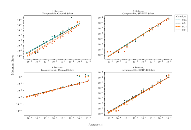
Figure 3: Effect of increasing $\alpha$ and $\epsilon$ on the maximum error recorded for the solver of an $8\times 8$ matrix for the four fluid cases considered here.

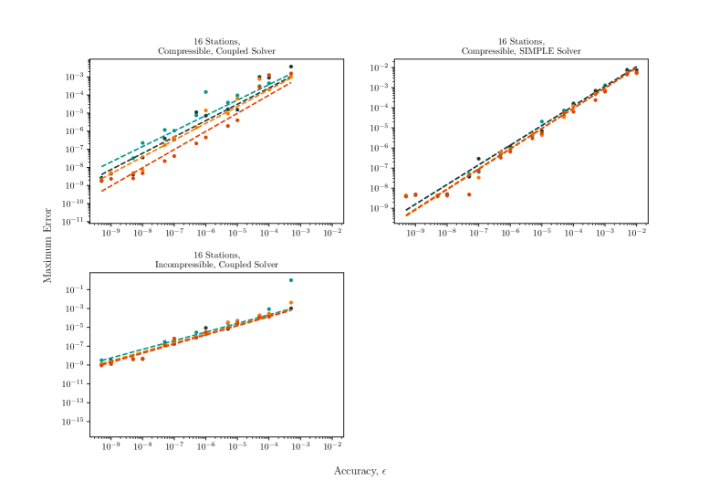
Figure 4: Effect of increasing $\alpha$ and $\epsilon$ on the maximum error recorded for the solver of an $16\times 16$ matrix for the compressible and incompressible fluid. The incompressible coupled solver has been omitted due to the time cost of obtaining enough unconverted results, many trials converged regardless of the value of $\alpha$.

V.2 Effect of Noisy Measurements on the QLES Solver

We can simulate the effect of using a QSVT algorithm with accuracy $\epsilon_{\textrm{meas}}$ and cutoff $\alpha$ as a subroutine in a classical CFD solver, to do this we run the outer loop of the CFD solver normally, but modify the corrections vector returned. First, we characterise the accuracy of the QSVT algorithm, $\epsilon_{\textrm{meas}}$ by applying a random Gaussian shift, described by a variance of $\epsilon_{\textrm{meas}}$ and mean of $0$ to the correction returned by the classical solver. We then modify the values of the correction vector using Equation 16.

The classical linear equation solver requires a tolerance $\epsilon_{\textrm{tol}}$, which stops the algorithm when the correction to at least one of the velocity, pressure, or compressible flow, $\rho$ are below $\epsilon_{\textrm{tol}}$. In preliminary investigations, we find that, without introducing an $\alpha$-cutoff (alternately $\alpha=0$), most cases of the solver converge if tolerance $=\epsilon_{\textrm{meas}}$. We are interested in the cases where $\epsilon_{\textrm{meas}}>\epsilon_{\textrm{tol}},\alpha>0$. For simplicity, we now only discuss the maximum correction (or error) returned over the three parameters of interest for the final correction vector. The final correction vector is returned when either the tolerance condition of the classical solver is met, or we have exceeded some number of total iterations, which for the results here is $10^{8}$ . We then set the tolerance of the classical algorithm to $1\times 10^{-9}$ and investigate the effect of increasing $\epsilon,\alpha$ on the maximum error.

In Figures 3 and  4 we show the effect of accuracy, $\epsilon_{\textrm{meas}}$, and cutoff value, $\alpha$, on the maximum error recorded for $s=8,16$ examples. Both accuracy and maximum error have been plotted on a log scale, and a linear fit has been drawn. We see that the maximum error in the correction vector rises when the accuracy is decreased, as can be expected. More interestingly, increasing the value of $\alpha$, i.e. measuring fewer amplitudes, seems to have a small effect on the final result. This means we can perform fewer measurements overall by setting $\alpha$ to high values, e.g. $\alpha=0.9$ for a moderate sacrifice in the maximum error. The coupled solutions in Figure 3 show some outliers for $\epsilon>10^{-3}$. These are cases where a low-precision feedback loop caused the non-linear solver to fail to converge [12]. All other cases converged to the desired accuracy.

Amplitude Estimation	Accuracy	$Stations$	Phase Factors	$\kappa$	Logical Qubits	Physical Qubits	T Gates	Toffoli Gates	Oracle Time (s)	Oracle Calls	Total Time (Days)	Percentage Of Amplitudes
True	$1\times 10^{-5}$	8	$8.83\times 10^{4}$	48.13	35	$4.23\times 10^{4}$	$7.21\times 10^{8}$	$1.59\times 10^{6}$	$8.73\times 10^{3}$	$4.29\times 10^{5}$	$4.34\times 10^{4}$	-
False	$1\times 10^{-5}$	8	$8.83\times 10^{4}$	48.13	35	$5.69\times 10^{4}$	$1.78\times 10^{8}$	$7.95\times 10^{5}$	$1.99\times 10^{3}$	$1.00\times 10^{10}$	$2.30\times 10^{8}$	100
True	$1\times 10^{-4}$	8	$7.68\times 10^{4}$	48.13	35	$4.23\times 10^{4}$	$5.83\times 10^{8}$	$1.38\times 10^{6}$	$7.07\times 10^{3}$	$4.00\times 10^{4}$	$3.27\times 10^{3}$	-
False	$1\times 10^{-4}$	8	$7.68\times 10^{4}$	48.13	35	$5.69\times 10^{4}$	$1.43\times 10^{8}$	$6.91\times 10^{5}$	$1.61\times 10^{3}$	$1.00\times 10^{8}$	$1.86\times 10^{6}$	100
True	$1\times 10^{-3}$	8	$6.53\times 10^{4}$	48.13	35	$4.23\times 10^{4}$	$4.58\times 10^{8}$	$1.17\times 10^{6}$	$5.56\times 10^{3}$	$3.61\times 10^{3}$	233	-
False	$1\times 10^{-3}$	8	$6.53\times 10^{4}$	48.13	35	$5.69\times 10^{4}$	$1.13\times 10^{8}$	$5.87\times 10^{5}$	$1.26\times 10^{3}$	$1.00\times 10^{6}$	$1.46\times 10^{4}$	100
True	0.01	8	$5.37\times 10^{4}$	48.13	35	$4.23\times 10^{4}$	$3.46\times 10^{8}$	$9.66\times 10^{5}$	$4.20\times 10^{3}$	304	15	-
False	0.01	8	$5.37\times 10^{4}$	48.13	35	$5.69\times 10^{4}$	$8.48\times 10^{7}$	$4.83\times 10^{5}$	954.20	$1.00\times 10^{4}$	111	43.75
True	$1\times 10^{-5}$	16	$2.57\times 10^{5}$	131.05	41	$4.61\times 10^{4}$	$4.20\times 10^{9}$	$5.65\times 10^{6}$	$5.49\times 10^{4}$	$4.29\times 10^{5}$	$2.73\times 10^{5}$	-
False	$1\times 10^{-5}$	16	$2.57\times 10^{5}$	131.05	41	$4.41\times 10^{4}$	$1.03\times 10^{9}$	$2.82\times 10^{6}$	$1.25\times 10^{4}$	$1.00\times 10^{10}$	$1.45\times 10^{9}$	100
True	$1\times 10^{-4}$	16	$2.25\times 10^{5}$	131.05	41	$4.61\times 10^{4}$	$3.44\times 10^{9}$	$4.95\times 10^{6}$	$4.49\times 10^{4}$	$4.00\times 10^{4}$	$2.08\times 10^{4}$	-
False	$1\times 10^{-4}$	16	$2.25\times 10^{5}$	131.05	41	$4.41\times 10^{4}$	$8.44\times 10^{8}$	$2.47\times 10^{6}$	$1.02\times 10^{4}$	$1.00\times 10^{8}$	$1.19\times 10^{7}$	100
True	$1\times 10^{-3}$	16	$1.93\times 10^{5}$	131.05	41	$4.61\times 10^{4}$	$2.74\times 10^{9}$	$4.25\times 10^{6}$	$3.59\times 10^{4}$	$3.61\times 10^{3}$	$1.50\times 10^{3}$	-
False	$1\times 10^{-3}$	16	$1.93\times 10^{5}$	131.05	41	$4.41\times 10^{4}$	$6.72\times 10^{8}$	$2.13\times 10^{6}$	$8.17\times 10^{3}$	$1.00\times 10^{6}$	$9.46\times 10^{4}$	100
True	0.01	16	$1.62\times 10^{5}$	131.05	41	$4.61\times 10^{4}$	$2.11\times 10^{9}$	$3.55\times 10^{6}$	$2.77\times 10^{4}$	304	98	-
False	0.01	16	$1.62\times 10^{5}$	131.05	41	$4.41\times 10^{4}$	$5.17\times 10^{8}$	$1.78\times 10^{6}$	$6.29\times 10^{3}$	$1.00\times 10^{4}$	729	21.88

Table 1: Resource requirements for the uncoupled compressible fluid in a nozzle scenario. Number of phase factors characterises how many phase factors are required to approximate $A^{-1}$ at accuracy $\epsilon$, $\kappa$ is the subnormalisation of the matrix to be inverted. Oracle time is the time taken to implement an amplitude encoding oracle where Amplitude Estimation is True, and a single QSVT circuit otherwise. Oracle calls is given by Equation 10 when Amplitude Estimation is True, and $\frac{1}{\epsilon^{2}}$ otherwise. Total time is oracle calls multiplied by oracle time. Percentage of amplitudes characterises the percentage of the basis vectors that can be measured using Amplitude Estimation in the time taken for the naive case.

VI Discussion

We have studied the use of amplitude estimation as a method of measuring outputs of a QSVT algorithm, specifically for CFD use cases. We have adapted the algorithm presented in [2] for use in a setting where the implemented unitary is itself a QSVT operator, and we have used the estimates given in [2] to estimate the number of times an operator needs to be measured to estimate a single correction peak from a CFD calculation. This allows us to estimate physical resources for a single amplitude.

The time resources required by this algorithm are daunting, especially when considering the fact that this is the inner loop of a CFD calculation. The idea introduced here, of using cut-off $\alpha$ reduces the number of times the algorithm will be used, but not the resources for a single implementation of matrix inversion. The number of phase factors required to implement the matrix inversion polynomial is the dominant factor in these circuits, reducing this number whilst maintaining $\epsilon_{inv}$ is the subject of future work. As the function approximating $A^{-1}$ is real, an antisymmetric list of phase factors is guaranteed to exist. However, whilst there has been recent advances in finding phase factors for polynomials [27, 28], this is not for an antisymmetric list. Work into constructing antisymmetric lists of phase factors will also be constructive.

Appendix A Resource Estimation Details

To produce the concrete resource requirements we must calculate the additional resources required for error correction once we have calculated the logical qubit and non-Clifford gate count. We must make some assumptions about the device to use, which is based on the surface code on a 2D grid, following the scheme given in “A Game of Surface Codes” [29].

We choose a target failure probability of $p_{\text{fail}}=1\%$ for a full execution of the quantum algorithm, which we divide into error budgets $p_{\text{fail}}^{\text{log}}=0.9\%$ for logical errors, and $p_{\text{fail}}^{\text{MSD}}=0.1\%$ for undetected errors in magic state distillation.

For the systems considered here, we use a two level magic state factory with asymmetric code distances, based on the scheme laid out in [30]. These factories produce high quality $T$ states using smaller magic state factories to input some lower quality distilled $T$ states. The longer circuits seen here use the (15-to-1)${}^{4}_{9,3,3}$ $\times$ (20-to-4)_15,7,9 factory from [30]. It has a sufficiently low failure probability, below the target error $p_{\text{fail}}^{\text{MSD}}/N_{\text{T}}$ A smaller code distance than $d$ in the logical computation can be used for the magic state factory to reduce its footprint and runtime. In fact, rectangular code patches with distinct distances for X, Z, and time (as indicated by the subscripts) can be used as the factory is more prone to some types of error than others.

Using the [29] scheme, we assume the computation proceeds as fast as consuming one magic state qubit per logical clock cycle, where a logical clock cycle is equivalent to $d$ code cycles, and $d$ is the code distance. Consequently, we ensure that the number of magic state factories available is high enough that a single magic state is available every logical cycle, which typically requires multiple magic state factories. The length of the computation is $N_{\text{T}}$ logical cycles.

The logical error budget bounds the allowed logical failure probability per logical cycle, which is given by the Fowler-Devitt-Jones formula [31]. Hence the computational code distance $d$ must be chosen such that

$$A\left(\frac{p}{p_{\textrm{thr}}}\right)^{\frac{d+1}{2}}\leq\frac{p_{\text{fail}}^{\text{log}}}{N_{\text{T}}N_{\textrm{qubits}}},$$ (18)

where $p$ is the probability of a physical error, $p_{\text{thr}}\approx 0.01$ is the threshold of the surface code, and $A=0.1$ is a numerically determined constant.

In order to estimate the physical resources, we model a 2D superconducting device, with an error rate one order of magnitude better than current superconducting devices [32, 33], i.e. $p=0.01\%$. This allows us to solve Equation 18 for $d$. The total number of logical qubits $n_{L}$ is given by the number of qubits required by the algorithm and the routing required by the fast-block layout [29, Figure 13]. The total number of physical qubits is then $(2d^{2}-1)n_{L}$ for algorithm and routing in the rotated surface code, together with those required by the magic state factories.

Appendix B Modelling $a_{\textrm{max}}$

To find a model of $a_{\textrm{max}}$ we first build some dummy quantum states with uniform output probabilities. For some total number of qubits $D\in[3,4,5,6]$ we create a dummy wavefunction with $2^{D}$ amplitudes. We choose a total number of peaks, $N_{\textrm{peaks}}\in[2^{d_{i}}]$ for $d_{i}\in\{0\dots D-1\}$, and at $N_{\textrm{peaks}}$ random basis vectors in the uniform state replace the amplitude with one of $a_{\textrm{max}}\in[0.25,0.5,0.75,0.9,0.99]$ and re-normalise the vector. This produces vectors like those in Figure 5.

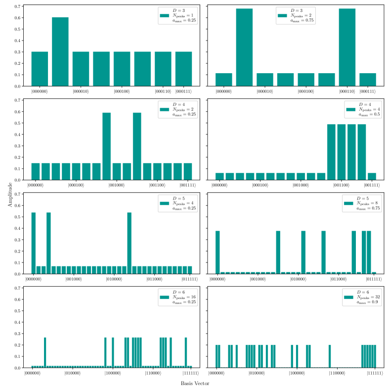
Figure 5: A selection of some of the basis vectors used to find a model for $a_{\textrm{max}}$, for different values of $D$ the number of qubits, $N_{\textrm{peaks}}$ a total number of high peaks, and $a_{\textrm{max}}$ values. $a_{\textrm{max}}$ is a relative value as these vectors have all been re-normalised.

We then simulate measurement of these wavefunctions by sampling for $N_{\textrm{shots}}\in[10,50,100,500,1\times 10^{3},5\times 10^{3},1\times 10^{4},5\times 10^{4},1\times 10^{5}]$ and recording the basis vector measured. We follow the algorithm detailed in Section IV.1, recording the number of unique basis vectors seen, $N_{\textrm{new}}$ and the ratio $r=\frac{N_{\textrm{new}}}{N_{S}}$. We can then plot this ratio against $N_{S}$ and draw a linear fit to it as in Figures 6 - 9.

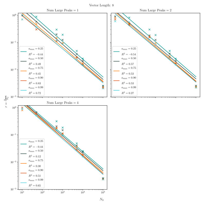
Figure 6: Linear fit to the ratio, $r=\frac{N_{\textrm{new}}}{N_{S}}$ against the total number of samples taken, $N_{S}$ for a 3 qubit output vector, differing numbers of large peaks and (un-normalised) $a_{\textrm{max}}$ values. We see there is a small dependence on the gradient of the fit on $a_{\textrm{max}}$, which suggests we can model it on aggregate.

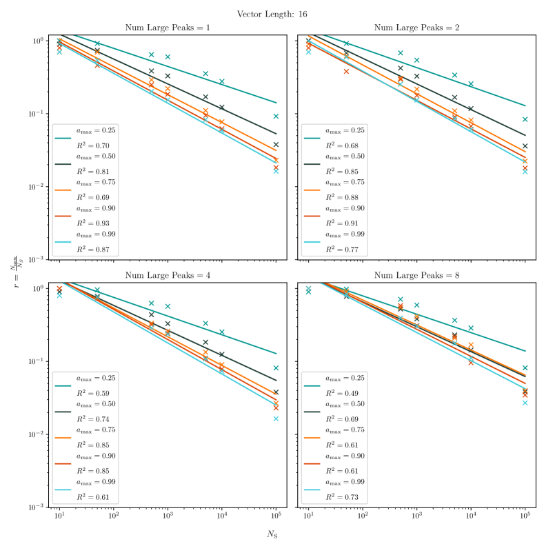
Figure 7: Linear fit to the ratio, $r=\frac{N_{\textrm{new}}}{N_{S}}$ against the total number of samples taken, $N_{S}$ for a 4 qubit output vector, differing numbers of large peaks and (un-normalised) $a_{\textrm{max}}$ values. We see there is a small dependence on the gradient of the fit on $a_{\textrm{max}}$, which suggests we can model it on aggregate.

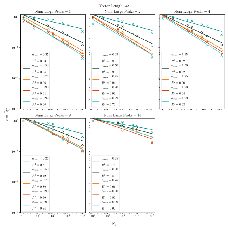
Figure 8: Linear fit to the ratio, $r=\frac{N_{\textrm{new}}}{N_{S}}$ against the total number of samples taken, $N_{S}$ for a 5 qubit output vector, differing numbers of large peaks and (un-normalised) $a_{\textrm{max}}$ values. We see there is a small dependence on the gradient of the fit on $a_{\textrm{max}}$, which suggests we can model it on aggregate.

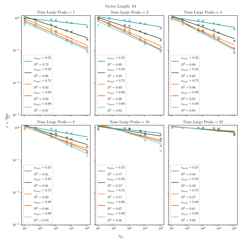
Figure 9: Linear fit to the ratio, $r=\frac{N_{\textrm{new}}}{N_{S}}$ against the total number of samples taken, $N_{S}$ for a 6 qubit output vector, differing numbers of large peaks and (un-normalised) $a_{\textrm{max}}$ values. We see there is a small dependence on the gradient of the fit on $a_{\textrm{max}}$, which suggests we can model it on aggregate.

We see that in many cases there is a relationship between the gradient of the fit line and $a_{\textrm{max}}$, with larger $a_{\textrm{max}}$ leading to a lower slope on the gradient. We can then model this dependence by averaging over all cases to plot the relationship between $\frac{dr}{dN_{S}}$ and $a_{\textrm{max}}$, and we draw a polynomial fit to this data. The polynomial fit is shown in Figure 10

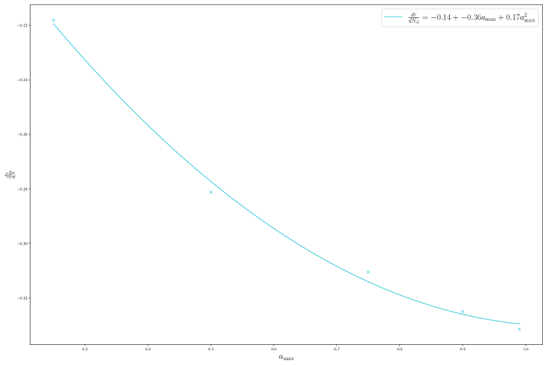
Figure 10: Polynomial fit of $\frac{dr}{dN}$ against $a_{\textrm{max}}$ which can be used to give an estimate of $a_{\textrm{max}}$ in the ‘burn-in’ period.

The polynomial fit is:

$$\frac{dr}{dN_{S}}=0.17a_{\textrm{max}}^{2}-0.36a_{\textrm{max}}-0.14.$$ (19)

This can be solved for some real instance of $\frac{dr}{dN_{S}}$ to give an estimate of $a_{\textrm{max}}$.

Appendix C Toeplitz Matrix Resource Estimation

In [26] a block encoding for the Toeplitz matrix, which has a wide number of potential applications, was introduced. Here we apply the same resource estimation used for the compressible and incompressible nozzle in the main text to the Toeplitz matrix.

Amplitude Estimation	Accuracy	$Stations$	Phase Factors	$\kappa$	Logical Qubits	Physical Qubits	T Gates	Toffoli Gates	Oracle Time (s)	Oracle Calls	Total Time (Days)	Percentage Of Amplitudes
True	$1\times 10^{-5}$	16	$1.31\times 10^{5}$	2.97	41	$4.41\times 10^{4}$	$5.14\times 10^{8}$	$5.78\times 10^{6}$	$6.45\times 10^{3}$	$4.29\times 10^{5}$	$3.20\times 10^{4}$	-
False	$1\times 10^{-5}$	16	$1.31\times 10^{5}$	2.97	41	$5.83\times 10^{4}$	$1.26\times 10^{8}$	$2.89\times 10^{6}$	$1.51\times 10^{3}$	$1.00\times 10^{10}$	$1.75\times 10^{8}$	100
True	$1\times 10^{-4}$	16	$1.11\times 10^{5}$	2.97	41	$4.41\times 10^{4}$	$4.03\times 10^{8}$	$4.88\times 10^{6}$	$5.07\times 10^{3}$	$4.00\times 10^{4}$	$2.35\times 10^{3}$	-
False	$1\times 10^{-4}$	16	$1.11\times 10^{5}$	2.97	41	$5.83\times 10^{4}$	$9.87\times 10^{7}$	$2.44\times 10^{6}$	$1.19\times 10^{3}$	$1.00\times 10^{8}$	$1.38\times 10^{6}$	100
True	$1\times 10^{-3}$	16	$9.06\times 10^{4}$	2.97	41	$4.41\times 10^{4}$	$3.03\times 10^{8}$	$3.98\times 10^{6}$	$3.83\times 10^{3}$	$3.61\times 10^{3}$	161	-
False	$1\times 10^{-3}$	16	$9.06\times 10^{4}$	2.97	41	$5.83\times 10^{4}$	$7.41\times 10^{7}$	$1.99\times 10^{6}$	902.50	$1.00\times 10^{6}$	$1.04\times 10^{4}$	100
True	0.01	16	$7.00\times 10^{4}$	2.97	41	$4.41\times 10^{4}$	$2.14\times 10^{8}$	$3.08\times 10^{6}$	$2.72\times 10^{3}$	304	10	-
False	0.01	16	$7.00\times 10^{4}$	2.97	41	$5.83\times 10^{4}$	$5.22\times 10^{7}$	$1.54\times 10^{6}$	641.80	$1.00\times 10^{4}$	75	43.75
True	$1\times 10^{-5}$	32	$9.74\times 10^{5}$	19.52	45	$4.75\times 10^{4}$	$4.03\times 10^{9}$	$4.48\times 10^{7}$	$5.47\times 10^{4}$	$4.29\times 10^{5}$	$2.72\times 10^{5}$	-
False	$1\times 10^{-5}$	32	$9.74\times 10^{5}$	19.52	45	$4.52\times 10^{4}$	$9.89\times 10^{8}$	$2.24\times 10^{7}$	$1.29\times 10^{4}$	$1.00\times 10^{10}$	$1.50\times 10^{9}$	100
True	$1\times 10^{-4}$	32	$8.40\times 10^{5}$	19.52	45	$4.75\times 10^{4}$	$3.25\times 10^{9}$	$3.87\times 10^{7}$	$4.42\times 10^{4}$	$4.00\times 10^{4}$	$2.04\times 10^{4}$	-
False	$1\times 10^{-4}$	32	$8.40\times 10^{5}$	19.52	45	$4.52\times 10^{4}$	$7.95\times 10^{8}$	$1.93\times 10^{7}$	$1.05\times 10^{4}$	$1.00\times 10^{8}$	$1.21\times 10^{7}$	100
True	$1\times 10^{-3}$	32	$7.06\times 10^{5}$	19.52	45	$4.75\times 10^{4}$	$2.53\times 10^{9}$	$3.25\times 10^{7}$	$3.46\times 10^{4}$	$3.61\times 10^{3}$	$1.44\times 10^{3}$	-
False	$1\times 10^{-3}$	32	$7.06\times 10^{5}$	19.52	45	$4.52\times 10^{4}$	$6.19\times 10^{8}$	$1.62\times 10^{7}$	$8.20\times 10^{3}$	$1.00\times 10^{6}$	$9.50\times 10^{4}$	100
True	0.01	32	$5.72\times 10^{5}$	19.52	45	$4.75\times 10^{4}$	$1.89\times 10^{9}$	$2.63\times 10^{7}$	$2.59\times 10^{4}$	304	92	-
False	0.01	32	$5.72\times 10^{5}$	19.52	45	$4.52\times 10^{4}$	$4.60\times 10^{8}$	$1.32\times 10^{7}$	$6.16\times 10^{3}$	$1.00\times 10^{4}$	713	21.88

Table 2: Resource requirements for the Toeplitz matrix use case. Number of phase factors characterises how many phase factors are required to approximate $A^{-1}$ at accuracy $\epsilon$, $\kappa$ is the subnormalisation of the matrix to be inverted. Oracle time is the time taken to implement an amplitude encoding oracle where Amplitude Estimation is True, and a single QSVT circuit otherwise. Oracle calls is given by Equation 10 when Amplitude Estimation is True, and $\frac{1}{\epsilon^{2}}$ otherwise. Total time is oracle calls multiplied by oracle time. Percentage of amplitudes characterises the percentage of the basis vectors that can be measured using Amplitude Estimation in the time taken for the naive case.

References

- [1] A. Gilyén, Y. Su, G. H. Low and N. Wiebe, Quantum singular value transformation and beyond: Exponential improvements for quantum matrix arithmetics, doi:10.1145/3313276.3316366 (2018).
- [2] P. Rall and B. Fuller, Amplitude Estimation from Quantum Signal Processing, Quantum 7, 937 (2023), doi:10.22331/q-2023-03-02-937.
- [3] P. W. Shor, Polynomial-Time Algorithms for Prime Factorization and Discrete Logarithms on a Quantum Computer, In AT&T Research, pp. 20–22. IEEE Computer Society Press (1994).
- [4] L. Lapworth, A Hybrid Quantum-Classical CFD Methodology with Benchmark HHL Solutions (2022), eprint 2206.00419.
- [5] D. F. V. James, P. G. Kwiat, W. J. Munro and A. G. White, On the Measurement of Qubits, Physical Review A 64(5), 052312 (2001), doi:10.1103/PhysRevA.64.052312, eprint quant-ph/0103121.
- [6] Z. Hradil, Quantum-state estimation, Physical Review A 55(3), R1561 (1997), doi:10.1103/PhysRevA.55.R1561.
- [7] G. Torlai, G. Mazzola, J. Carrasquilla, M. Troyer, R. Melko and G. Carleo, Many-body quantum state tomography with neural networks, Nature Physics 14(5), 447 (2018), doi:10.1038/s41567-018-0048-5, eprint 1703.05334.
- [8] M. Cramer, M. B. Plenio, S. T. Flammia, R. Somma, D. Gross, S. D. Bartlett, O. Landon-Cardinal, D. Poulin and Y.-K. Liu, Efficient quantum state tomography, Nature Communications 1(1), 149 (2010), doi:10.1038/ncomms1147.
- [9] Z. M. Rossi, J. L. Ceroni and I. L. Chuang, Modular quantum signal processing in many variables, doi:10.48550/arXiv.2309.16665 (2023), eprint 2309.16665.
- [10] A. Manzano, D. Musso and A. Leitao, Real quantum amplitude estimation, EPJ Quantum Technology 10(1), 1 (2023), doi:10.1140/epjqt/s40507-023-00159-0.
- [11] N. Hills, Achieving high parallel performance for an unstructured unsteady turbomachinery CFD code, The Aeronautical Journal 111(1117), 185 (2007), doi:10.1017/S0001924000004449.
- [12] L. Lapworth, Implicit Hybrid Quantum-Classical CFD Calculations using the HHL Algorithm, doi:10.48550/arXiv.2209.07964 (2022), eprint 2209.07964.
- [13] A. Gilyén, Y. Su, G. H. Low and N. Wiebe, Quantum singular value transformation and beyond: Exponential improvements for quantum matrix arithmetics, In Proceedings of the 51st Annual ACM SIGACT Symposium on Theory of Computing, pp. 193–204. ACM, Phoenix AZ USA, ISBN 978-1-4503-6705-9, doi:10.1145/3313276.3316366 (2019).
- [14] G. Brassard, P. Hoyer, M. Mosca and A. Tapp, Quantum Amplitude Amplification and Estimation, doi:10.1090/conm/305/05215 (2002), eprint quant-ph/0005055.
- [15] L. K. Grover, From Schrödinger’s equation to the quantum search algorithm, Pramana - Journal of Physics 56(2-3), 333 (2001), doi:10.1119/1.1359518.
- [16] A. Kitaev, Quantum measurements and the Abelian Stabilizer Problem, Tech. Rep. TR96-003, Electronic Colloquium on Computational Complexity (ECCC) (1996).
- [17] S. Aaronson and P. Rall, Quantum Approximate Counting, Simplified, In 2020 Symposium on Simplicity in Algorithms (SOSA), Proceedings, pp. 24–32. Society for Industrial and Applied Mathematics, doi:10.1137/1.9781611976014.5 (2019).
- [18] Y. Suzuki, S. Uno, R. Raymond, T. Tanaka, T. Onodera and N. Yamamoto, Amplitude estimation without phase estimation, Quantum Information Processing 19(2), 75 (2020), doi:10.1007/s11128-019-2565-2.
- [19] C.-R. Wie, Simpler quantum counting, Quantum Information and Computation 19(11&12), 967 (2019), doi:10.26421/QIC19.11-12-5.
- [20] M. Dobsicek, G. Johansson, V. S. Shumeiko and G. Wendin, Arbitrary accuracy iterative phase estimation algorithm as a two qubit benchmark, Physical Review A 76(3), 030306 (2007), doi:10.1103/PhysRevA.76.030306, eprint quant-ph/0610214.
- [21] D. Grinko, J. Gacon, C. Zoufal and S. Woerner, Iterative quantum amplitude estimation, npj Quantum Information 7(1), 1 (2021), doi:10.1038/s41534-021-00379-1.
- [22] A. Callison and D. E. Browne, Improved maximum-likelihood quantum amplitude estimation, doi:10.48550/arXiv.2209.03321 (2023), eprint 2209.03321.
- [23] K. Mizuta and K. Fujii, Recursive Quantum Eigenvalue/Singular-Value Transformation: Analytic Construction of Matrix Sign Function by Newton Iteration, doi:10.48550/arXiv.2304.13330 (2023), eprint 2304.13330.
- [24] Z. M. Rossi and I. L. Chuang, Semantic embedding for quantum algorithms, doi:10.48550/arXiv.2304.14392 (2023), eprint 2304.14392.
- [25] V. V. Shende, S. S. Bullock and I. L. Markov, Synthesis of Quantum Logic Circuits, IEEE Transactions on Computer-Aided Design of Integrated Circuits and Systems 25(6), 1000 (2006), doi:10.1109/TCAD.2005.855930, eprint quant-ph/0406176.
- [26] C. Sünderhauf, E. Campbell and J. Camps, Block-encoding structured matrices for data input in quantum computing, Quantum 8, 1226 (2024), doi:10.22331/q-2024-01-11-1226.
- [27] B. K. Berntson and C. Sünderhauf, Complementary polynomials in quantum signal processing, doi:10.48550/arXiv.2406.04246 (2024), eprint 2406.04246.
- [28] M. Alexis, L. Lin, G. Mnatsakanyan, C. Thiele and J. Wang, Infinite quantum signal processing for arbitrary Szegő functions (2024), doi:10.48550/arXiv.2407.05634, eprint 2407.05634.
- [29] D. Litinski, A Game of Surface Codes: Large-Scale Quantum Computing with Lattice Surgery, Quantum 3, 128 (2019), doi:10.22331/q-2019-03-05-128.
- [30] D. Litinski, Magic State Distillation: Not as Costly as You Think, arXiv:1905.06903 [quant-ph] (2019), eprint 1905.06903.
- [31] A. G. Fowler, M. Mariantoni, J. M. Martinis and A. N. Cleland, Surface codes: Towards practical large-scale quantum computation, Physical Review A - Atomic, Molecular, and Optical Physics 86(3) (2012), doi:10.1103/PhysRevA.86.032324.
- [32] R. Acharya, I. Aleiner, R. Allen, T. I. Andersen, M. Ansmann, F. Arute, K. Arya, A. Asfaw, J. Atalaya, R. Babbush, D. Bacon, J. C. Bardin et al., Suppressing quantum errors by scaling a surface code logical qubit, Nature 614(7949), 676 (2023), doi:10.1038/s41586-022-05434-1.
- [33] S. Krinner, N. Lacroix, A. Remm, A. Di Paolo, E. Genois, C. Leroux, C. Hellings, S. Lazar, F. Swiadek, J. Herrmann, G. J. Norris, C. K. Andersen et al., Realizing repeated quantum error correction in a distance-three surface code, Nature 605(7911), 669 (2022), doi:10.1038/s41586-022-04566-8.