Intensity correlations in decoy-state BB84 quantum key distribution systems

Abstract

The decoy-state method is a prominent approach to enhance the performance of quantum key distribution (QKD) systems that operate with weak coherent laser sources. Due to the limited transmissivity of single photons in optical fiber, current experimental decoy-state QKD setups increase their secret key rate by raising the repetition rate of the transmitter. However, this usually leads to correlations between subsequent optical pulses. This phenomenon leaks information about the encoding settings, including the intensities of the generated signals, which invalidates a basic premise of decoy-state QKD. Here we characterize intensity correlations between the emitted optical pulses in two industrial prototypes of decoy-state BB84 QKD systems and show that they significantly reduce the asymptotic key rate. In contrast to what has been conjectured, we experimentally confirm that the impact of higher-order correlations on the intensity of the generated signals can be much higher than that of nearest-neighbour correlations.

I Introduction

Quantum key distribution (QKD) represents a method for achieving information-theoretic security when sharing a confidential bit string, commonly referred to as a secret key, between distant parties Bennett and Brassard (1984); Xu et al. (2020); Lo et al. (2014); Pirandola et al. (2020). Despite its theoretical security being rigorously proven Lo and Chau (1999); Shor and Preskill (2000); Koashi (2009); Renner (2008), practical implementations of QKD encounter challenges and limitations associated with current technology Brassard et al. (2000); Xu et al. (2020), which might lead to security loopholes, or so-called side channels Makarov et al. (2006); Zhao et al. (2008); Lydersen et al. (2010); Gerhardt et al. (2011); Huang et al. (2019, 2020); Ruzhitskaya et al. (2021); Ye et al. (2023). To address these discrepancies between theory and practice, manufacturers of QKD equipment can apply improved security proofs that can handle device imperfections Gottesman et al. (2004); Lo et al. (2014); Lim et al. (2014); Tamaki et al. (2014); Pereira et al. (2020); Marquardt et al. ; Currás-Lorenzo et al. and/or incorporate advanced hardware solutions Dixon et al. (2017); Ponosova et al. (2022); Makarov et al. . Alternatively, the development and adoption of novel QKD protocols and methods, inherently resilient to specific vulnerabilities and quantum hacking attempts, offer another avenue. For example, measurement-device-independent (MDI) QKD closes all measurement loopholes without the need for theoretical characterization of the measurement unit Lo et al. (2012). Additionally, employing a twin-field (TF) QKD protocol has demonstrated the potential to significantly extend the achievable distance Lucamarini et al. (2018); Minder et al. (2019); Wang et al. (2019); Zhong et al. (2019); Wang et al. (2022); Liu et al. (2023).

Nevertheless, despite these notable accomplishments, challenges remain to be addressed before QKD can attain widespread adoption as a technology Xu et al. (2015); Diamanti et al. (2016); Xu et al. (2020). A crucial hurdle involves enhancing the secret key rate produced by existing experimental prototypes, a task affected significantly by the restricted transmissivity of single photons in optical fibers and the dead time of the receivers’ detectors. For this reason, various experimental demonstrations have been conducted with an increased pulse repetition rate of the sources of several gigahertz Grünenfelder et al. (2020); Boaron et al. (2018). Yet, within such a high-speed domain, the presence of memory effects in the optical modulators and their controlling electronics establishes correlations among the generated optical pulses, thus invalidating most security proofs. Significantly, this phenomenon introduces a security vulnerability in the form of information leakage. Fortunately, various security proofs have recently addressed the problem of pulse correlations Pereira et al. (2020); Zapatero et al. (2021); Sixto et al. (2022); Pereira et al. (2023); Currás-Lorenzo et al. (2023); Pereira et al. , but they require a precise characterization of the source.

On the experimental side, a few recent works have quantified the strength of pulse correlations for various particular QKD system prototypes Grünenfelder et al. (2020); Yoshino et al. (2018); Kang et al. (2023); Lu et al. (2023), and showed that such correlations are, in general, not negligible. However, more experimental efforts are needed to accurately characterize pulse correlations of arbitrary order in QKD systems that are already available on the market.

In this work, we experimentally study intersymbol intensity correlations in two industrial prototypes of decoy-state BB84 systems developed by two different vendors. We observe strong intensity correlations in both setups and apply a security proof that considers this imperfection Sixto et al. (2022). In doing so, we quantify the impact of this potential loophole on their performance in terms of secret key rate (SKR). Surprisingly, we find that in some cases higher-order correlations may affect the intensity of the emitted pulses more than nearest-neighbour correlations.

The paper is organized as follows. In Section II, we introduce the experimental setup we use to characterize the intensity correlations and describe the measurement procedure. There, we also explain the QKD protocol employed by the systems and define the assumptions we apply in the experiment. In Section III, we present the experimental results revealing the intersymbol intensity correlations problem in both QKD systems studied. We then apply the security proof recently developed in Sixto et al. (2022), which takes into account this imperfection, and obtain asymptotic secret key rates in Sec. IV. We conclude in Sec. V. The paper also includes a methods section with additional calculations.

II Experimental setup and measurements

We measure and analyze the intensities of modulated non-attenuated optical pulses produced by the source unit (Alice) of the two QKD systems considered. We shall refer to them as system A and system B. Although each of these systems is a complete engineering solution with its elaborately developed technical features, their crucial optical and electrical elements are similar. Figure 1(a) introduces one conceptual scheme that is accurate for the measurement sessions in both setups.

Figure 1: Correlation measurement. (a) Simplified scheme of the measurement setup for intensity correlations. Alice generates optical pulses with a laser diode (Laser). These pulses propagate through an intensity modulator (IM) and an encoding modulator (EM) and obtain a random intensity and encoding state according to the prescriptions of a decoy-state BB84 protocol. Both modulators are controlled with a field-programmable gate array (FPGA) that sets different operating voltage levels according to the signal received from a (quantum) random number generator (Q)RNG (one of the Alices tested is equipped with a classical pseudo-RNG). To ensure a classical energy level of the optical pulses at Alice’s output, we remove a variable optical attenuator (VOA) from the optical scheme. The measurement setup consists of a fast photodetector (PD) and a digital high-bandwidth oscilloscope (OSC). (b) Conceptual view of five consecutive optical pulses emitted by Alice. The intensity of the latest-emitted correlated pulse D depends on the previously emitted pulses, whose number determines the correlation length $\xi$. In this work, we shall consider correlations up to $\xi=6$. (c) A short fragment of the recorded data oscillogram measured on system B with five registered consecutive optical pulses. The intensity settings and the chronological order of the pulses are the same as in (b). Dashed lines and arrows highlight the deviations in the maximum amplitude values of the D intensity setting pulses. (d) Distributions of calculated energies for the studied intensity settings (gray) and $\xi=1$ in system B. Each intensity setting, denoted by X, is represented by four distributions. We normalize the energy by the mean value of the S-state distribution. (e) Zoomed-in fragment of (d) with decoy-state distributions. We show both unnormalized (top) and normalized (bottom) groups of distributions. The latter group is normalized such that each distribution area’s integral equals 1. The mean value for each distribution is marked by a vertical line of the same color. From these distributions, it follows that, in general, SD pulses have less energy than DD or VD pulses. The same trend can also be seen in (c).

Both systems run a decoy-state BB84 protocol with three intensity settings Lo et al. (2005); Ma et al. (2005). The applied intensity setting to the $k$-th pulse produced by system A (system B) is $a_{k_{A}}\in A_{A}=\{\mu_{A},\nu_{A},\omega_{A}\}$ ($a_{k_{B}}\in A_{B}=\{\mu_{B},\nu_{B},\omega_{B}\}$) with probability $p_{a_{k_{A}}}$ ($p_{a_{k_{B}}}$), where $p_{\mu_{A}}>p_{\nu_{A}}>p_{\omega_{A}}$ ($p_{\mu_{B}}>p_{\nu_{B}}\geq p_{\omega_{B}}$). The relation between the intensity levels in system A (system B) is $\mu_{A}>\nu_{A}>\omega_{A}\geq 0$ ($\mu_{B}>\nu_{B}>\omega_{B}\geq 0$), where $\mu$ represents the signal state (S), $\nu$ is the decoy state (D), and $\omega$ is the vacuum state (V).

Performance speed restrictions and memory effects affect the core elements of Alice’s setup that are involved in the preparation of the optical pulses she sends to Bob. These core elements include electro-optical modulators, high-speed electrical drivers, control motherboards, and CPUs. Due to these implementation limitations, an increase in the repetition rate of a QKD system can cause correlations between the emitted optical pulses. Hence, several parameters of an emitted optical pulse (i.e., intensity, polarization, and phase) may depend on the parameters chosen to code the previously emitted pulses. In Fig. 1(b) we illustrate the concept of intensity correlations. We remark that, although this parameter is commonly labeled “intensity” in the literature on QKD, it actually represents the energy of the optical pulse. Figure 1(b) presents five consecutive optical pulses emitted by Alice with three intensity settings. In this model, the latest-emitted D pulse is correlated with the preceding pulses. The exact number of such pulses that condition the intensity of this D pulse is the correlation length $\xi$. The simplest case is first-order pulse correlations (i.e., $\xi=1$), or so-called nearest-neighbour correlations, which correspond to the scenario where the intensity of a pulse depends on the intensity of the previous pulse [SD pattern in Fig. 1(b)]. Similarly, the intensity of a pulse can be influenced by even earlier-emitted pulses along with its nearest neighbour. In our example, this corresponds to second-order ($\xi=2$, pattern DSD), third-order ($\xi=3$, pattern DDSD), and fourth-order ($\xi=4$, pattern VDDSD) correlations. While $\xi$ can in principle be arbitrarily large in a QKD system, in our work we limit the value of $\xi$ to 4 (6) for system A (B), because the confidence intervals become too large for the higher values of $\xi$ in the measured data set. Nevertheless, our analysis can be straightforwardly adapted to any large value of $\xi$.

Following Fig. 1(a), in the measurement session, Alice of system A (system B) generates phase-randomized coherent pulses with a repetition rate of $40~{}\mathrm{M}\mathrm{Hz}$ (several hundred $\mathrm{M}\mathrm{Hz}$). Each of them is randomly modulated by an intensity modulator according to the prescriptions of the decoy-state BB84 protocol with three intensity settings. Then, the pulses pass through an encoding modulator (EM) and are randomly encoded in the BB84 states. To measure the intensity of the produced states, we connect Alice’s output to a fast photodetector Picometrix PT-40A with DC to $38$-$\mathrm{G}\mathrm{Hz}$ bandwidth (Thorlabs RXM40AF with $300$-$\mathrm{k}\mathrm{Hz}$ to $40\mbox{-}\mathrm{G}\mathrm{Hz}$ bandwidth), which in turn is coupled to a digital oscilloscope Agilent DSOX93304Q with $33$-$\mathrm{G}\mathrm{Hz}$ analog bandwidth and $80$-$\mathrm{G}\mathrm{Hz}$ sampling rate (LeCroy SDA816Zi with $16$-$\mathrm{G}\mathrm{Hz}$ analog bandwidth and $40$-$\mathrm{G}\mathrm{Hz}$ sampling rate). The experimental data is recorded in the form of high-resolution voltage oscillograms with $12.5$ $(25)~{}\mathrm{p}\mathrm{s}$ sampling period for system A (system B), containing hundreds of thousands of pulses. We show an example of the experimental data in Fig. 1(c). The shown data fragment consists of five consecutive optical pulses produced by system B, which match the intensity settings presented in the concept scheme illustrated in Fig. 1(b). We mark the maximum amplitude value for each D pulse with dashed lines and highlight the difference with arrows. This difference hints that the intensities of the produced optical pulses are correlated.

We additionally process the raw experimental data and eliminate the instrument noise. An unfiltered noise can contribute to the energy calculation results and, therefore, bias the conclusion about the presence of correlations in a QKD system. We use the combination of digital filters based on Savitzky-Golay Savitzky and Golay (1964); Bromba and Ziegler (1981) and singular value decomposition (SVD) techniques Grassberger et al. (1993); Konstantinides et al. (1997); Jha and Yadava (2011); Huang et al. (2023) (see Methods A for details). We calculate the energy of each registered denoised pulse by integrating its area over a fixed time window. Then, from the calculated energy value we determine the pulse’s intensity setting. After that, we compute the distributions of pulses’ energies for each studied intensity pattern ($3^{\xi+1}$ distributions in total for each analyzed system). As an example, in Fig. 1(d), we present the energy distributions for all $\xi=1$ patterns together with the overall distributions of pulses’ energies for each intensity setting (gray) for system B. Moreover, we show a zoomed-in sector with decoy-state pulses’ energies distributions and their mean values in Fig. 1(e). In Section III we compare these mean values to ascertain whether intensity correlations exist in the systems under study.

Assumptions

We make the following assumptions during the measurements and data processing.

Assumption 1. We define the intersymbol intensity correlations by observing the recorded energies of bright non-attenuated optical pulses. We assume that the correlations at the single-photon level of energy are the same as those observed at the classical level of optical energy. From our point of view, the optical attenuation is not an active process and should not contribute to intensity correlations, since the energy of each attenuated pulse is reduced equally and independently of each other.

Assumption 2. Since we make our analysis based on experimentally measured values of the optical energy, we assume that our measurement equipment converts the optical power into digital values linearly. Precisely, we consider that the optical-to-electrical conversion in the classical photoreceiver and the voltage measurement in the oscilloscope are linear. While these radio-frequency electronics in fact have non-linearities, we assume they do not significantly affect our results.

Assumption 3. To make sure that instrument noise components do not contribute to the resulting energy calculations, we utilize digital filtering based on the Savitzky-Golay Savitzky and Golay (1964); Bromba and Ziegler (1981) and SVD Grassberger et al. (1993); Konstantinides et al. (1997); Jha and Yadava (2011); Huang et al. (2023) techniques. We assume they effectively eliminate the instrument noise while keeping the true signal values unchanged.

Assumption 4. The noise floor in the measured data is about $0~{}\mathrm{V}$, or even slightly below this value as shown in Fig. 1(c). While this is a consequence of the typical unavoidable effect of non-ideal measurement device calibration and instrument noise, it results in negative values when calculating the energy for V pulses, which obviously has no physical meaning and is a problem for secret key rate calculations. We overcome this issue by adding the lowest negative energy value found within our experimental sequence to each calculated pulse energy. This guarantees that all the pulses in the data set have energy greater or equal to zero after this operation. While this does not affect the experimental results and calculated energy distributions, it can slightly affect the calculation of the secret key rates. We believe that this operation is necessary and we assume that its effect on the secret key rate calculation is negligible.

III Results

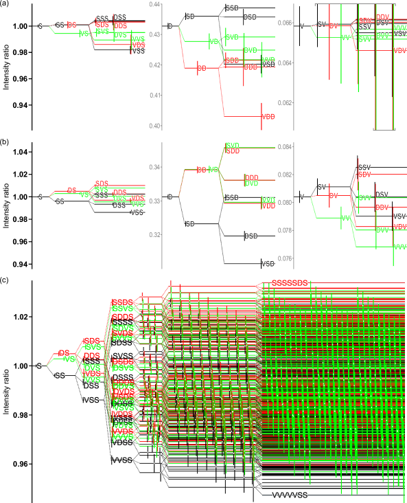
Figure 2: Measured intensity correlations in (a) system A and (b) system B up to second order ($\xi=2$). Each horizontal line represents the mean value of energy distribution for a state preceded by a certain pattern of states. The value is normalized to the mean of S (gray vertical scales) or the mean of the state plotted (black vertical scale, applies to all three sets). The vertical line to the left of each label represents the confidence interval for a confidence level of $0.9$. The experimental results for the S states of system B are extended up to $\xi=6$ in (c). The most separated patterns associated to sixth order correlations are labeled and their waveforms are analyzed in Fig. 3(a) and (b). Owing to the lack of figure space, in (c) we plot confidence intervals at the sixth order only for those patterns derived from VS (green). We also provide additional calculated ratios in Methods D.

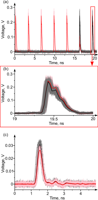
Figure 3: Comparison of averaged oscillogram waveforms of the two most-intensity-separated patterns, (a) measured in system B—SSSSSDS (red solid line) and VVVVVSS (black solid line). Individual measured pulses are plotted in pink (SSSSSDS, 250 pulses) and gray (VVVVVSS, 250 pulses). A noticeable deviation in the waveforms of the S state when considering $\xi=6$ is additionally shown in the zoomed-in sector (b). A similar effect of the long correlations on the pulses’ waveforms is observed in system A as well (c). In the latter, we compare the waveforms of the most separated decoy-state third-order patterns—DSSD (black and gray, 50 pulses) and VVDD (red and pink, 50 pulses).

We analyze a recorded sequence containing 171120 S states, 28240 D states, and 24201 V states produced by system A (509267 S, 255433 D, and 254139 V states produced by system B) that we collected during the measurement. We present the central experimental result in Fig. 2. We show the intensity ratios for the first- and second-order correlations for both systems in Fig. 2(a) and (b). Here each horizontal line represents the mean energy of the state preceded by the pattern of states, in relative (black vertical scale) and absolute (gray vertical scales) units. The last letter of each label indicates the intensity setting of the analyzed state. That is, the vertical position of every labeled line represents the intensity ratio given by

$$\text{position}_{\text{rel}} =\frac{\langle\text{pattern}\rangle}{\langle\text{setting}\rangle}\text{ on the black global scale;}$$ (1a)

$$\text{position}_{\text{abs}} =\frac{\langle\text{pattern}\rangle}{\langle S\rangle}\text{ on the gray local scale.}$$ (1b)

Here, $\langle\text{pattern}\rangle$ is the mean energy of the last pulse in the labeled pattern, $\langle\text{setting}\rangle$ is the mean energy of the corresponding one-letter distribution, and $\langle S\rangle$ is the mean energy of S for a given QKD system. In Methods A we provide examples illustrating how the intensity ratios are calculated. For each system, there are 39 horizontal lines: 3 of them have one-letter labels and show the mean of the energy distribution of all pulses with the intensity setting S, D, or V; 9 have two letters in the label and represent the mean of the energy distribution for each $\xi=1$ pattern; finally, 27 labeled with three letters represent each $\xi=2$ pattern. According to Fig. 2(a) and (b), intensity correlations are present in both studied QKD systems, with setting D being the most affected by them. Furthermore, as can be seen from the same figure, the deviations of the second-order patterns for the S and D settings in both systems are either similar or even greater than those corresponding to nearest-neighbour correlations. We examine this long correlation effect even more in Fig. 2(c), where we illustrate the intensity ratios for the S states of system B up to $\xi=6$. While it is commonly assumed that the first-order correlations should have the greatest impact on the intensity of the correlated state, our findings suggest that the largest deviations between intensities correspond to the third-order correlated patterns. Moreover, as can be seen from the same figure, the strength of the correlations decreases relatively slowly with an increase of the order of correlation length, making a noticeable impact even in the fifth- and sixth-order correlated patterns. We note that, for the latter order, we plot the confidence intervals only for the patterns derived from the VS state, which is the “worst-case” scenario with the largest intervals. The energy deviations caused by the intensity correlations are almost indistinguishable for these patterns, while for the ones derived from SS or DS, the sixth-order deviations are still statistically significant. We compare the waveforms of the higher-order labeled pattern pulses for both systems in Fig. 3. The waveforms of different intensity clearly tend to have different amplitude and shape.

In the perfect scenario, when a QKD system does not have intensity correlations, all the patterns presented in Fig. 2 should form one single horizontal line at the relative intensity ratio of 1. Clearly, this is not the case. A possible reason for the existence of such relatively large correlations in the decoy setting patterns is an unstable working point of the intensity modulator while encoding the decoy states Lu et al. (2021). Typically, the operating voltages for the vacuum and signal states are chosen to be at the extremes of the $\cos^{2}$-shaped modulator transfer function, which are quite stable positions. On the other hand, the decoy state modulating voltage is placed at the slope of the transfer function, and any small voltage fluctuation results in relatively high encoded intensity deviations.

IV Effect on the security of QKD

IV.1 Theoretical analysis

To account for the influence of intensity correlations in the decoy-state method, we apply the security analysis presented in Sixto et al. (2022); Zapatero et al. (2021), based on the so-called Cauchy-Schwarz (CS) constraint Lo and Preskill (2007); Pereira et al. (2020); Zapatero et al. (2021). This result is used to upper-bound the bias that Eve can induce between the detection statistics of Fock states with different records of intensity settings. In what follows, we elaborate on the details of this parameter estimation technique for the case of nearest-neighbour pulse correlations, $\xi=1$, and the reader is referred to Sixto et al. (2022) for further details.

Firstly, we list the three assumptions on which the analysis relies.

(i) For any given round $k$ and photon number $n_{k}$, there exists a physical intensity $\alpha_{k}$ such that

$$p\left(n_{k}|\alpha_{k}\right)=\frac{e^{-\alpha_{k}}\alpha_{k}^{n_{k}}}{n_{k}!}.$$ (2)

Namely, the photon-number statistics are Poissonian conditioned on the value of the physical intensity. This feature is supported by recent high-speed QKD experiments Yoshino et al. (2018); Grünenfelder et al. (2020).

(ii) $\alpha_{k}$ is a bounded random variable for all $k$ and its distribution $g_{a_{k},a_{k-1}}$ is determined by the present setting, $a_{k}$, and the neighbouring setting, $a_{k-1}$. As a consequence,

$$\left.p_{n_{k}}\right|_{a_{k},a_{k-1}}=\int_{a_{k}^{-}}^{a_{k}^{+}}g_{a_{k},a_{k-1}}(\alpha_{k})\frac{e^{-\alpha_{k}}\alpha_{k}^{n_{k}}}{n_{k}!}d\alpha_{k},$$ (3)

for all $n_{k}$. Note that, without loss of generality, the boundaries can be expressed as $a_{k}^{\pm}=a_{k}\left(1\pm\delta^{\pm}_{a_{k},a_{k-1}}\right)$ for some relative deviations $\delta^{\pm}_{a_{k},a_{k-1}}$ with respect to $a_{k}$.

(iii) The intensity correlations have a finite range $\xi$. The value of the physical intensity of round $k$, $\alpha_{k}$, is only affected by those previous settings $a_{j}$ with $k-j\leq\xi$. We note that this assumption could be removed by using the recent results in Pereira et al. .

Importantly, the above assumptions enable the desired parameter estimation, summarized in Methods B.

IV.2 Asymptotic secret key rate simulations

Frequently, the post-selection technique Renner (2007); Renner and Cirac (2009) is invoked to justify the asymptotic equivalence between the secret key rates with collective and coherent attacks. However, in the presence of pulse correlations, a necessary round-exchangeability property of the post-selection technique is invalidated. In a similar way, correlations invalidate the counterfactual argument often invoked under ideal decoy-state preparation Zapatero et al. (2021). Hence, a different approach must be followed to define an (as general as possible) asymptotic regime. Particularly, if the variances of the experimental averages vanish asymptotically, the secret key rate can be estimated as Zapatero et al. (2021)

$$K_{\infty}=\mathrm{bar}{Z}_{1,\mu,N}^{\mathrm{L}}\left[1-h\left(\frac{\mathrm{bar}{E}_{1,\mu,N}^{\mathrm{U}}}{\mathrm{bar}{X}_{1,\mu,N}^{\mathrm{L}}}\right)\right]-f_{\mathrm{EC}}\mathrm{bar}{Z}_{\mu,N}h\left(E_{\mathrm{tol}}\right),$$ (4)

for a large enough number of rounds $N$ Zapatero et al. (2021), where $\mathrm{bar}{Z}_{1,\mu,N}^{\mathrm{L}}$ ($\mathrm{bar}{X}_{1,\mu,N}^{\mathrm{L}}$) provides a lower bound on the average number of signal-setting single-photon counts among those events in which both Alice and Bob select the $Z$ ($X$) basis, and $\mathrm{bar}{E}_{1,\mu,N}^{\mathrm{U}}$ provides an upper bound on the average number of signal-setting single-photon error counts among those events in which both users select the $X$ basis. Also, $h(x)$ denotes the binary entropy, $f_{\mathrm{EC}}$ stands for the error correction efficiency, $\mathrm{bar}{Z}_{\mu,N}$ is defined as $\mathrm{bar}{Z}_{\mu,N}={Z}_{\mu,N}/N$ for $Z_{\mu,N}=\sum_{c\in A}Z_{\mu,c,N}$, $Z_{\mu,c,N}$ denoting the number of $Z$ basis counts associated to the record of settings $(a_{k},a_{k-1})=(\mu,c)$ and $E_{\mathrm{tol}}$ denotes the overall error rate observed in the $Z$ basis. The quantities $\mathrm{bar}{Z}_{1,\mu,N}^{\mathrm{L}}$, $\mathrm{bar}{X}_{1,\mu,N}^{\mathrm{L}}$ and $\mathrm{bar}{E}_{1,\mu,N}^{\mathrm{U}}$ can be estimated from the observed gains and error gains via linear programming, as shown in Zapatero et al. (2021); Sixto et al. (2022).

To evaluate the performance of both systems, we assume a truncated Gaussian (TG) distribution for the correlation function $g_{a_{k},a_{k-1}}$, which is observed in Fig. 1(d) and (e) and also motivated by previous studies Yoshino et al. (2018); Huang et al. (2023). Regardless, the analysis presented below is applicable to any other distribution function. For each system, we set the ratios between the intensity settings, the maximum relative deviations, and the mean and variance of the TG distributions following the experimental values provided in Methods D. The asymptotic secret key rates calculated is plotted in Figs. 4 and 5 for $\xi=1$ and $\xi=2$. For system B, we vary the average intensity of the signal setting $\mu$, which would physically correspond to setting the attenuation of Alice’s variable optical attenuator (VOA). The ratios between the intensities and the minimum and maximum deviations are still obtained from Table 2. Note that the signals from system A could also be further attenuated to improve performance, but since that system already emits signals at the single-photon level, we opt not to include this additional step.

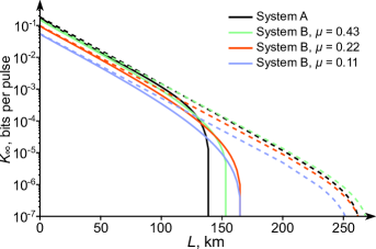
Figure 4: Asymptotic secret key rate $K_{\infty}$ for the case of first-order pulse correlations ($\xi=1$, solid lines) and for the ideal scenario without correlations ($\xi=0$, dashed lines). For system B, we consider different attenuations to study the dependence of the secret key rate on the decoy state intensities. It is apparent from the figure that lowering the intensities in the presence of correlations is beneficial for long-distance transmissions. For the simulations, we use the channel model described in Methods C.

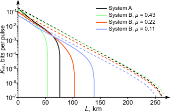
Figure 5: Asymptotic secret key rate $K_{\infty}$ for the case of second-order pulse correlations ($\xi=2$, solid lines) and for the ideal scenario without correlations ($\xi=0$, dashed lines). Similarly to Fig. 4, we consider different values of the attenuation for system B and we use the channel model presented in Methods C.

As can be seen in the plots, increasing the attenuation (i.e., lowering the intensities) is beneficial for long-distance transmission. Considering $\xi=2$ substantially impairs the performance. While for $\xi\geq 3$ a non-zero key rate is expected for both systems, we do not include results for these higher-order simulations, as we believe that the first two orders are sufficient to demonstrate the general methodology.

V Conclusion

We have experimentally demonstrated the presence of long intensity correlations between the optical pulses produced by two different decoy-state BB84 QKD systems. The impact of higher-order correlations on the pulse’s intensity is similar or higher than that of the nearest-neighbour case, even at relatively low sub-gigahertz pulse repetition rates. As discussed in previous literature, this effect challenges a fundamental assumption underlying most decoy-state security proofs, posing a potential threat to the reliability of QKD systems. To address this issue, we have introduced a simple method for measuring the relevant quantities to accurately characterize intensity correlations, and we have assessed their impact on the secret key rate for the first- and second-order correlations. Our findings indicate that intensity correlations could substantially impair the performance of decoy-state QKD. Furthermore, we have shown that the secret key rate is highly sensitive to the output mean photon number and ratios between the different intensities. We believe that vendors can optimize these parameters to minimize the effect of intensity correlations on QKD performance. Another strategy could be increasing the bandwidth of the electro-optical devices responsible for the intensity modulation in Alice. Also, we suggest that electrical and optical lines used with these devices should be carefully characterized to avoid parasitic interference, such as multiple back-and-forth reflections in the cables. A preliminary study shows correlations in the electrical signal feeding the modulator Trefilov (2021).

Methods

Methods A Data processing

To transform the raw oscillogram data collected with the measurement setup [see Fig. 1(c)] to the form presented in Fig. 2, we process the data and apply several filtering techniques to it, namely SVD (for S and D states) and Savitzky-Golay (for V states) digital filters. This is explained below, together with the procedure to calculate the resulting intensity ratios and their confidence intervals shown in Fig. 2.

SVD filtering. To apply the SVD filtering method, we populate a matrix $M$ with $n$ recorded oscillograms of noisy pulses of the same intensity setting and width $m$ (the number of points that make up the waveform), so that $M=n\times m$. We can decompose $M$ as

$$M=USV^{\top},$$ (5)

where $U$ is an $m\times m$ unitary matrix with its columns being left singular vectors, $S$ is an $m\times n$ diagonal matrix with singular values placed in descending order, and $V^{\top}$ is an $n\times n$ unitary matrix, whose rows are right singular vectors. The initial noisy data in the $M$ matrix after the decomposition is transformed into singular values of the $S$ diagonal matrix. A magnificent property of the SVD method is that the singular values that characterize a waveform of the true measured signal are the first large values of $S$, while the singular values of an independent and individually distributed (i.i.d.) Gaussian instrument noise are relatively small and spread along its $m$ dimension. The core idea of the SVD filtering method is that after the decomposition, it is possible to separate the subspaces of true signal singular values from those of the noise, and then one can remove the latter. We show the singular values for all intensity settings in both systems in Fig. 6 and indicate the ones that we make zero. As a result, a new diagonal matrix $S^{\prime}$ can be constructed, with only a few orders of non-zero descending singular values. Then, one can perform the inverse operation of the decomposition to obtain the reconstructed matrix $M^{\prime}$, populated with filtered optical pulses

$$M^{\prime}=US^{\prime}V^{\top}.$$ (6)

After this operation, each row of the resulting matrix $M^{\prime}$ represents the filtered optical pulse, the noisy version of which was previously contained in the initial matrix $M$. Since the singular values for the V states are relatively low and indistinguishable from those of noise, we cannot filter these optical pulses with this type of filter, so we apply another technique based on the Savitzky-Golay approach, which we present next.

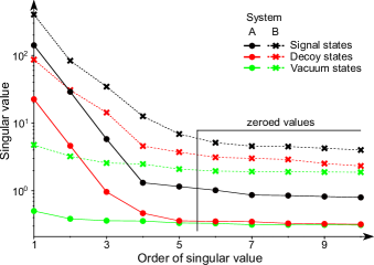
Figure 6: The first ten orders of singular values of all intensity settings for both examined systems. To remove the noise, we make zero the singular values of the $S$ matrices corresponding to the S and D pulses after the fifth order of singular values.

Savitzky-Golay filtering. To filter the recorded vacuum states from the instrument noise, we employ a technique based on a well-known Savitzky-Golay digital low-pass filter with predefined optimized parameters Savitzky and Golay (1964); Bromba and Ziegler (1981). This method is based on a local least-squares low-degree polynomial approximation, and, similarly to the moving-average filter, it smooths the noisy oscillograms by locally fitted polynomial functions at every point of the experimental data. As a result, the distorted signal is smoothed, while the shape of recorded waveforms is maintained. We show an example of the vacuum state before and after filtering in Fig. 7. For both systems, we optimize and put the degree of fitting polynomial function as 3, and the width of the filtration window as 39 experimental points.

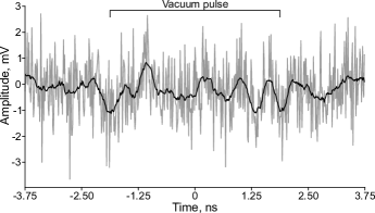
Figure 7: An oscillogram of the single vacuum state measured on system A before (gray) and after (black) Savitzky-Golay filtering.

Calculation of confidence intervals. For clarity, in what follows we provide the confidence intervals for the case of nearest-neighbour correlations, and the generalization to higher-order correlations is straightforward. Let us consider the set of all rounds $k$ such that: (i) setting $a$ is selected in round $k$ and (ii) setting $c$ is selected in round $k-1$. We shall assume that the intensities measured in any two rounds of this set are independent random variables. Under this assumption, one can infer a confidence interval on the population mean of the set $\langle\alpha_{ac}\rangle$, given the sample mean $\mathrm{bar}{\alpha}_{ac}$, using Hoeffding’s inequality. Particularly, for a confidence level of $1-\delta$, the interval reads

$$I_{ac}=[\mathrm{bar}{\alpha}_{ac}-\Delta_{\delta/2},\mathrm{bar}{\alpha}_{ac}+\Delta_{\delta/2}],$$ (7)

where $\Delta_{\delta/2}=w_{ac}\sqrt{\ln(2/\delta)/2N_{ac}}$, $N_{ac}$ is the number of patterns $ac$ in the data set, and $w_{ac}$ denotes the maximum range among all random variables in the set. Since the theoretical ranges are unknown, to estimate $I_{ac}$ we replace $w_{ac}$ with the difference between the largest and the smallest measured intensities in the set. For the confidence intervals that we plot in Figs. 2 and 8 we fix the value of $\delta=0.1$.

Examples of calculation. Here, we briefly explain how we calculate the vertical positions of the lines plotted in Fig. 2 for D, VS, and SDV patterns of the system A. According to Eqs. 1a and 1b,

$$\begin{split}D_{\text{rel}}&=\frac{\langle D\rangle}{\langle D\rangle}=1,\\ VS_{\text{rel}}&=\frac{\langle VS\rangle}{\langle S\rangle}=\frac{0.635059}{0.638635}\approx 0.9944,\\ SDV_{\text{rel}}&=\frac{\langle SDV\rangle}{\langle V\rangle}=\frac{0.042150}{0.042044}\approx 1.0025,\end{split}$$ (8)

$$\begin{split}D_{\text{abs}}&=\frac{\langle D\rangle}{\langle S\rangle}=\frac{0.276372}{0.638635}\approx 0.4328,\\ VS_{\text{abs}}&=\frac{\langle VS\rangle}{\langle S\rangle}=\frac{0.635059}{0.638635}\approx 0.9944,\\ SDV_{\text{abs}}&=\frac{\langle SDV\rangle}{\langle S\rangle}=\frac{0.042150}{0.638635}\approx 0.06600.\end{split}$$ (9)

The values we use in these equations are average energies for distributions of corresponding patterns that we converted into photons for system A (arbitrary units for system B). We provide this data for all patterns and both QKD systems in Methods D.

Methods B Parameter estimation technique

In this section, we present the derivation of the necessary constraint to estimate the relevant parameters via linear programming Zapatero et al. (2021); Sixto et al. (2022).

For any given round $k$ and photon-number $n$, the yield and the error probability associated to the pair of settings $(a_{k},a_{k-1})=(a,c)$ are defined as

$$Y_{n,a,c}^{(k)}=p(s_{k}\neq f|$$ (10)

$$n_{k}=n,a_{k}=a,a_{k-1}=c,x_{k}=Z,y_{k}=Z),$$

$$H_{n,a,c,r}^{(k)}=p(s_{k}\neq f,s_{k}\neq r_{k}|$$

$$n_{k}=n,a_{k}=a,a_{k-1}=c,x_{k}=X,y_{k}=X,r_{k}=r),$$

where $x_{k}\in\{X,Z\}$, $r_{k}\in\{0,1\}$ represent the key bits selected by Alice, $y_{k}\in\{X,Z\}$ represents Bob’s basis selection, $s_{k}$ stands for Bob’s classical outcome, and $f$ represents a “no-click” event.

In virtue of the CS constraint, for any pair of distinct settings $a$ and $b$ in round $k$, and for any setting $c$ in round $k-1$, the associated yields and error probabilities satisfy

$$G_{-}\!\left(Y_{n,a,c}^{(k)},\tau_{a,b,c,n}\right)\leq Y_{n,b,c}^{(k)}\leq G_{+}\!\left(Y_{n,a,c}^{(k)},\tau_{a,b,c,n}\right)$$ (11)

and

$$G_{-}\!\left(H_{n,a,c,r}^{(k)},\tau_{a,b,c,n}\right)\leq H_{n,b,c,r}^{(k)}\leq G_{+}\!\left(H_{n,a,c,r}^{(k)},\tau_{a,b,c,n}\right)\!,$$ (12)

where

$$G_{-}(y,z)=\begin{cases}g_{-}(y,z)&\text{ if }y>1-z\\ 0&\text{ otherwise }\end{cases},$$ (13)

$$G_{+}(y,z)=\begin{cases}g_{+}(y,z)&\text{ if }y<z\\ 1&\text{ otherwise }\end{cases},$$

and the functions $g_{\pm}(y,z)=y+(1-z)(1-2y)\pm 2\sqrt{z}(1-z)y(1-y)$. That is, Eqs. 11 and 12 quantify how much $Y_{n,b,c}^{(k)}$ and $H_{n,b,c,r}^{(k)}$ can deviate from $Y_{n,a,c}^{(k)}$ and $H_{n,a,c,r}^{(k)}$, respectively. Crucially, $\tau_{a,b,c,n}$ is the overlap parameter, representing a lower bound on the squared overlap between the two quantum states underlying the two yields that enter the constraints (see Sixto et al. (2022) for further details).

The fact that $g_{a_{k}a_{k-1}}$ follows a truncated Gaussian distribution, allows to derive explicit formulas for the overlap parameter in Eqs. 11 and 12, and the photon-number statistics of LABEL:pns. As shown in Sixto et al. (2022), the overlap can be computed with the following formula

$$\tau_{a,b,c,n}^{\xi=1}=\left[\sum_{a_{k+1}\in A}p_{a_{k+1}}\sum_{n_{k+1}=0}^{n_{\text{cut}}}\sqrt{p_{n_{k+1}}|_{a_{k+1},a}p_{n_{k+1}}|_{a_{k+1},b}}\right]^{2},$$ (14)

where $a_{k+1}$ is the setting selected in round $k+1$ and $p_{a_{k+1}}$ represents the probability of selecting such setting. Moreover, the CS constraints can be linearized so as not to break the linear character of the parameter estimation. Importantly, when applying the linearization step to the constraints in Eq. 11 [Eq. 12], an additional reference yield (error) parameter needs to be incorporated (see Zapatero et al. (2021); Sixto et al. (2022) for more details). In these works, the authors do not optimize these parameters to maximize the key rate, as they take the reference yield (reference error) as the one that can be expected by the behavior of the channel, neglecting the effect of correlations. This leads to a severe drop in performance, especially when the outputs of the linear programs and the reference parameters are mutually distant. To fix this and improve the secret key rate, we use the outputs of the linear programs at a certain distance point $L$ as the reference values for the next distance point $L+1$. For the first point, $L=0$, we find a close-to-optimal reference value by running the linear program multiple times with different reference parameters, and using the highest output. Importantly, the linear constraints represent a valid bound regardless of the reference value used.

As for the decoy-state constraints, their derivation is rather standard, and they can be written as

$$\frac{\left\langle\mathrm{bar}{Z}_{a,c,N}\right\rangle}{q_{\mathrm{Z}}^{2}p_{a}p_{c}}\geq\sum_{n=0}^{n_{cut}}p_{n|a,c}y_{n,a,c,N},$$ (15)

$$\frac{\left\langle\mathrm{bar}{Z}_{a,c,N}\right\rangle}{q_{\mathrm{Z}}^{2}p_{a}p_{c}}\leq 1-\sum_{n=0}^{n_{cut}}p_{n|a,c}+\sum_{n=0}^{n_{cut}}p_{n|a,c}y_{n,a,c,N},$$

and

$$\frac{\left\langle\mathrm{bar}{E}_{a,c,N}\right\rangle}{q_{\mathrm{X}}^{2}p_{a}p_{c}}\geq\sum_{n=0}^{n_{cut}}p_{n|a,c}h_{n,a,c,N},$$ (16)

$$\frac{\left\langle\mathrm{bar}{E}_{a,c,N}\right\rangle}{q_{\mathrm{X}}^{2}p_{a}p_{c}}\leq 1-\sum_{n=0}^{n_{cut}}p_{n|a,c}+\sum_{n=0}^{n_{cut}}p_{n|a,c}h_{n,a,c,N}.$$

Here, $q_{Z(X)}$ denotes the probability of selecting the $Z$ ($X$) basis, $p_{a}$ denotes the probability of selecting setting $a\in{}A$ in any given round, and the average yields and error probabilities are defined as $y_{n,a,c,N}=\sum_{k=1}^{N}Y_{n,a,c}^{(k)}/{N}$ and $h_{n,a,c,N}=\sum_{k=1}^{N}H_{n,a,c}^{(k)}/{N}$ for all possible settings. Also, we recall that the average gains are $\mathrm{bar}{Z}_{a,c,N}=Z_{a,c,N}/{N}$ for all possible inputs, and we have defined the average error gains as $\mathrm{bar}{E}_{a,c,N}=E_{a,c,N}/{N}$ where $E_{a,c,N}$ represents the error gain associated to settings $(a,c)$ and the number of rounds $N$.

Table 1: Experimental values for system A. All the values are converted into photons.

Pattern	$\mu$	$\sigma$	min energy	max energy
S	0.638635	0.025245	0.5286737	0.75879511
D	0.276372	0.011834	0.2332107	0.32248299
V	0.042044	0.011438	0	0.0870799
SS	0.639209	0.02523	0.5341994	0.75879511
SD	0.278423	0.011295	0.2332107	0.32248299
SV	0.042104	0.011465	0	0.0870799
DS	0.639251	0.025164	0.5332007	0.73899578
DD	0.267539	0.011064	0.2353542	0.3072787
DV	0.042053	0.0114	0.0003578	0.08378114
VS	0.635059	0.024665	0.5286737	0.74574953
VD	0.273149	0.010465	0.2373067	0.31787876
VV	0.041681	0.011308	0.0095704	0.08159895
SSS	0.641041	0.02466	0.5341994	0.75879511
SSD	0.280194	0.010597	0.2394827	0.32248299
SSV	0.042127	0.011459	0	0.08584321
SDS	0.640664	0.024714	0.5332007	0.73899578
SDD	0.269188	0.010417	0.2358168	0.30376055
SDV	0.042168	0.011334	0.0003578	0.08238706
SVS	0.635516	0.02442	0.5286737	0.74086963
SVD	0.274081	0.010288	0.2373067	0.31787876
SVV	0.041628	0.011378	0.0095704	0.08159895
DSS	0.641269	0.024331	0.5344015	0.75844048
DSD	0.278274	0.010504	0.2431097	0.31491301
DSV	0.042238	0.011337	0.0052164	0.08045127
DDS	0.640541	0.024997	0.5598773	0.72400049
DDD	0.26778	0.01083	0.24119	0.3072787
DDV	0.04226	0.011751	0.0058803	0.08378114
DVS	0.635509	0.024512	0.5545599	0.74574953
DVD	0.271324	0.010368	0.2466763	0.30586557
DVV	0.04174	0.011159	0.0112804	0.07264567
VSS	0.627076	0.02533	0.5379419	0.73671844
VSD	0.268378	0.010408	0.2332107	0.31405785
VSV	0.04183	0.011623	0.0016062	0.0870799
VDS	0.629704	0.025812	0.5388653	0.7387814
VDD	0.257378	0.009283	0.2353542	0.28204715
VDV	0.041267	0.011361	0.0054174	0.07010183
VVS	0.631902	0.025994	0.5338721	0.73724771
VVD	0.269303	0.010501	0.2380967	0.3014277
VVV	0.041942	0.011024	0.011866	0.07716827

Table 2: Experimental values in arbitrary units for system B normalized to the mean value of S.

Pattern	$\mu$	$\sigma$	min energy	max energy
S	1	0.03082	0.83158619	1.16027652
D	0.331205	0.031052	0.19323125	0.45560021
V	0.080408	0.019021	0	0.17750194
SS	0.996082	0.030962	0.83158619	1.11589638
SD	0.32323	0.030018	0.19323125	0.42464045
SV	0.081123	0.01879	0.00200947	0.17750194
DS	1.004939	0.030197	0.88605649	1.16027652
DD	0.339161	0.030004	0.24043238	0.44989812
DV	0.080498	0.019254	0	0.17635141
VS	1.002882	0.030115	0.87277413	1.11230916
VD	0.339283	0.029979	0.23637931	0.45560021
VV	0.078888	0.019157	0.00130488	0.1677094
SSS	1.002422	0.030046	0.86989206	1.11589638
SSD	0.331017	0.029067	0.23296353	0.42464045
SSV	0.082523	0.018923	0.00378569	0.17750194
SDS	1.010071	0.029604	0.89394137	1.1189707
SDD	0.34559	0.029354	0.24230907	0.44989812
SDV	0.082017	0.019482	0	0.16690062
SVS	1.007758	0.029584	0.89158475	1.11210491
SVD	0.345728	0.029272	0.24372433	0.45560021
SVV	0.080346	0.019318	0.00130488	0.1677094
DSS	0.993388	0.030198	0.83158619	1.09894054
DSD	0.319657	0.028884	0.20888549	0.42075485
DSV	0.080396	0.01868	0.00217222	0.15755742
DDS	1.002537	0.029783	0.88605649	1.10954641
DDD	0.336109	0.029079	0.24827166	0.43495529
DDV	0.079659	0.018802	0.00307564	0.17635141
DVS	1.000633	0.029598	0.88648747	1.11230916
DVD	0.336097	0.029045	0.23993033	0.43421851
DVV	0.07803	0.018938	0.01017669	0.15310763
VSS	0.986114	0.030495	0.86121691	1.10345797
VSD	0.311454	0.028425	0.19323125	0.41074145
VSV	0.079018	0.018386	0.00200947	0.15432216
VDS	0.996976	0.02977	0.88986999	1.16027652
VDD	0.329286	0.029034	0.24043238	0.42393855
VDV	0.078274	0.018972	0.00509359	0.14976811
VVS	0.995446	0.029884	0.87277413	1.1006765
VVD	0.329591	0.029173	0.23637931	0.42357123
VVV	0.076824	0.018809	0.01018254	0.15123735

Complementing these constraints with the ones in Eqs. 11 and 12 we can readily bound the key-rate parameters $\mathrm{bar}{Z}_{1,\mu,N}^{\mathrm{L}}$, $\mathrm{bar}{X}_{1,\mu,N}^{\mathrm{L}}$ and $\mathrm{bar}{E}_{1,\mu,N}^{\mathrm{U}}$ via linear programming. As an example, $\mathrm{bar}{Z}_{1,\mu,N}^{\mathrm{L}}$ is computed minimizing the average number of signal-setting single-photon counts among those events where Alice and Bob select the $Z$ basis, which is given by

$$\langle\mathrm{bar}{Z}_{1,\mu,N}\rangle=\sum_{h\in A}q_{\mathrm{Z}}^{2}p_{\mu}p_{h}p^{(k)}(1|\mu,h)y_{1,\mu,h,N}$$ (17)

restricted to the above constraints.

Methods C Channel model

Let $\eta_{\mathrm{det}}$ denote the common detection efficiency of Bob’s detectors, and let $\eta_{\mathrm{ch}}=10^{-\alpha_{\text{att}}L/10}$ be the transmittance of the quantum channel, where $\alpha_{\mathrm{att}}$ represents the attenuation coefficient of the fiber and $L$ (km) is the distance. Also, let $p_{\mathrm{d}}$ denote the dark count probability of each of Bob’s detectors and let $\delta_{A}$ stand for the polarization misalignment occurring in the channel. For the simulations presented in Figs. 4 and 5, we use the values $\eta_{\mathrm{det}}=0.65$, $\alpha_{\mathrm{att}}=0.2~{}\mathrm{d}\mathrm{B}\mathrm{/}\mathrm{k}\mathrm{m}$, $p_{\mathrm{d}}=7.2\times 10^{-8}$, and $\delta_{A}=0.08$, which are taken from Yin et al. (2016).

As shown in Sixto et al. (2022), a standard model yields

$$\frac{\left\langle\mathrm{bar}{Z}_{a,c,N}\right\rangle}{q_{\mathrm{Z}}^{2}p_{a}p_{c}}=\frac{\left\langle\mathrm{bar}{X}_{a,c,N}\right\rangle}{q_{\mathrm{X}}^{2}p_{a}p_{c}}=1-\left(1-p_{\mathrm{d}}\right)^{2}e^{-\eta a}$$ (18)

and

$$\frac{\left\langle\mathrm{bar}{E}_{a,c,N}\right\rangle}{q_{X}^{2}p_{a}p_{c}} = \frac{\left\langle\mathrm{bar}{E}_{a,c,N(\mathrm{Z})}\right\rangle}{q_{Z}^{2}p_{a}p_{c}}=\frac{p_{\mathrm{d}}^{2}}{2}+p_{\mathrm{d}}\left(1-p_{\mathrm{d}}\right)$$ (19)

$$\times \left(1+h_{\eta,a,c,\delta_{\mathrm{A}}}\right)+\left(1-p_{\mathrm{d}}\right)^{2}$$

$$\times \left(\frac{1}{2}+h_{\eta,a,c,\delta_{\mathrm{A}}}-\frac{1}{2}e^{-\eta a}\right),$$

where $\eta=\eta_{\mathrm{det}}\eta_{\mathrm{ch}}$ represents the total attenuation and $a,c\in A$. The parameter $h_{\eta,a,c,\delta_{\mathrm{A}}}$ is defined as $h_{\eta,a,c,\delta_{\mathrm{A}}}=\frac{1}{2}(e^{-\eta a\cos^{2}\delta_{\mathrm{A}}}-e^{-\eta a\sin^{2}\delta_{\mathrm{A}}})$ and $\mathrm{bar}{E}_{a,c,N(\mathrm{Z})}$ is equivalent to $\mathrm{bar}{E}_{a,c,N}$ but referred to the $Z$-basis error clicks instead. The tolerated bit error rate of the sifted key is set to $E_{\mathrm{tol}}=\left\langle\mathrm{bar}{E}_{\mu,N(\mathrm{Z})}\right\rangle/\left\langle\mathrm{bar}{Z}_{\mu,N}\right\rangle$.

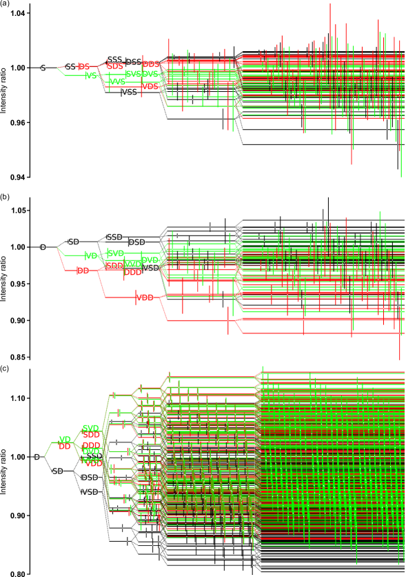
Figure 8: Measured intensity correlations of (a) the S and (b) the D states of system A, and (c) the D states of system B. The vertical lines represent the confidence intervals for a confidence level of $0.9$.

Methods D Experimental data values

We provide the experimental values that characterize the studied intensity patterns’ distributions for system A (system B) in Table 1 (Table 2). The represented parameters are the mean energy value $\mu$, standard deviation $\sigma$, and minimum and maximum energy values in a given distribution. All the described parameters are converted to be in photons (arbitrary units) for system A (system B) and correspond to the truncated Gaussian distributions. We also plot intensity ratios for the S and D states of system A and the D state of system B in Fig. 8.

References

- Bennett and Brassard (1984) C. H. Bennett and G. Brassard, “Quantum cryptography: Public key distribution and coin tossing,” in Proc. International Conference on Computers, Systems, and Signal Processing (IEEE Press, New York, Bangalore, India, 1984) pp. 175–179.
- Xu et al. (2020) F. Xu, X. Ma, Q. Zhang, H.-K. Lo, and J.-W. Pan, “Secure quantum key distribution with realistic devices,” Rev. Mod. Phys. 92, 025002 (2020).
- Lo et al. (2014) H.-K. Lo, M. Curty, and K. Tamaki, “Secure quantum key distribution,” Nat. Photonics 8, 595–604 (2014).
- Pirandola et al. (2020) S. Pirandola, U. L. Andersen, L. Banchi, M. Berta, D. Bunandar, R. Colbeck, D. Englund, T. Gehring, C. Lupo, C. Ottaviani, J. L. Pereira, M. Razavi, J. Shamsul Shaari, M. Tomamichel, V. C. Usenko, G. Vallone, P. Villoresi, and P. Wallden, “Advances in quantum cryptography,” Adv. Opt. Photonics 12, 1012–1236 (2020).
- Lo and Chau (1999) H.-K. Lo and H. F. Chau, “Unconditional security of quantum key distribution over arbitrarily long distances,” Science 283, 2050–2056 (1999).
- Shor and Preskill (2000) P. W. Shor and J. Preskill, “Simple proof of security of the BB84 quantum key distribution protocol,” Phys. Rev. Lett. 85, 441–444 (2000).
- Koashi (2009) M. Koashi, “Simple security proof of quantum key distribution based on complementarity,” New J. Phys. 11, 045018 (2009).
- Renner (2008) R. Renner, “Security of quantum key distribution,” Int. J. Quantum Inf. 6, 1–127 (2008).
- Brassard et al. (2000) G. Brassard, N. Lütkenhaus, T. Mor, and B. C. Sanders, “Limitations on practical quantum cryptography,” Phys. Rev. Lett. 85, 1330–1333 (2000).
- Makarov et al. (2006) V. Makarov, A. Anisimov, and J. Skaar, “Effects of detector efficiency mismatch on security of quantum cryptosystems,” Phys. Rev. A 74, 022313 (2006), erratum ibid. 78, 019905 (2008).
- Zhao et al. (2008) Y. Zhao, C.-H. F. Fung, B. Qi, C. Chen, and H.-K. Lo, “Quantum hacking: Experimental demonstration of time-shift attack against practical quantum-key-distribution systems,” Phys. Rev. A 78, 042333 (2008).
- Lydersen et al. (2010) L. Lydersen, C. Wiechers, C. Wittmann, D. Elser, J. Skaar, and V. Makarov, “Hacking commercial quantum cryptography systems by tailored bright illumination,” Nat. Photonics 4, 686–689 (2010).
- Gerhardt et al. (2011) I. Gerhardt, Q. Liu, A. Lamas-Linares, J. Skaar, C. Kurtsiefer, and V. Makarov, “Full-field implementation of a perfect eavesdropper on a quantum cryptography system,” Nat. Commun. 2, 349 (2011).
- Huang et al. (2019) A. Huang, Á. Navarrete, S.-H. Sun, P. Chaiwongkhot, M. Curty, and V. Makarov, “Laser-seeding attack in quantum key distribution,” Phys. Rev. Appl. 12, 064043 (2019).
- Huang et al. (2020) A. Huang, R. Li, V. Egorov, S. Tchouragoulov, K. Kumar, and V. Makarov, “Laser-damage attack against optical attenuators in quantum key distribution,” Phys. Rev. Appl. 13, 034017 (2020).
- Ruzhitskaya et al. (2021) D. D. Ruzhitskaya, I. V. Zhluktova, M. A. Petrov, K. A. Zaitsev, P. P. Acheva, N. A. Zunikov, A. V. Shilko, D. Aktas, F. Johlinger, D. O. Trefilov, A. A. Ponosova, V. A. Kamynin, and V. V. Makarov, “Vulnerabilities in the quantum key distribution system induced under a pulsed laser attack,” Sci. Tech. J. Inf. Technol. Mech. Opt. 21, 837–847 (2021), in Russian.
- Ye et al. (2023) P. Ye, W. Chen, G.-W. Zhang, F.-Y. Lu, F.-X. Wang, G.-Z. Huang, S. Wang, D.-Y. He, Z.-Q. Yin, G.-C. Guo, and Z.-F. Han, “Induced-photorefraction attack against quantum key distribution,” Phys. Rev. Appl. 19, 054052 (2023).
- Gottesman et al. (2004) D. Gottesman, H.-K. Lo, N. Lütkenhaus, and J. Preskill, “Security of quantum key distribution with imperfect devices,” Quantum Inf. Comput. 4, 325–360 (2004).
- Lim et al. (2014) C. C. W. Lim, M. Curty, N. Walenta, F. Xu, and H. Zbinden, “Concise security bounds for practical decoy-state quantum key distribution,” Phys. Rev. A 89, 022307 (2014).
- Tamaki et al. (2014) K. Tamaki, M. Curty, G. Kato, H.-K. Lo, and K. Azuma, “Loss-tolerant quantum cryptography with imperfect sources,” Phys. Rev. A 90, 052314 (2014).
- Pereira et al. (2020) M. Pereira, G. Kato, A. Mizutani, M. Curty, and K. Tamaki, “Quantum key distribution with correlated sources,” Sci. Adv. 6, eaaz4487 (2020).
- (22) Christoph Marquardt, Ulrich Seyfarth, Sven Bettendorf, Martin Bohmann, Alexander Buchner, Marcos Curty, Dominique Elser, Silas Eul, Tobias Gehring, Nitin Jain, Thomas Klocke, Marie Reinecke, Nico Sieber, Rupert Ursin, Marc Wehling, and Henning Weier, “Implementation attacks against QKD systems,” BSI technical report, https://www.bsi.bund.de/EN/Service-Navi/Publikationen/Studien/QKD-Systems/Implementation_Attacks_QKD_Systems_node.html, visited 3 Aug 2024.
- (23) G. Currás-Lorenzo, M. Pereira, G. Kato, M. Curty, and K. Tamaki, “A security framework for quantum key distribution implementations,” arXiv:2305.05930 [quant-ph] .
- Dixon et al. (2017) A. R. Dixon, J. F. Dynes, M. Lucamarini, B. Fröhlich, A. W. Sharpe, A. Plews, W. Tam, Z. L. Yuan, Y. Tanizawa, H. Sato, S. Kawamura, M. Fujiwara, M. Sasaki, and A. J. Shields, “Quantum key distribution with hacking countermeasures and long term field trial,” Sci. Rep. 7, 1978 (2017).
- Ponosova et al. (2022) A. Ponosova, D. Ruzhitskaya, P. Chaiwongkhot, V. Egorov, V. Makarov, and A. Huang, “Protecting fiber-optic quantum key distribution sources against light-injection attacks,” PRX Quantum 3, 040307 (2022).
- (26) Vadim Makarov, Alexey Abrikosov, Poompong Chaiwongkhot, Aleksey K. Fedorov, Anqi Huang, Evgeny Kiktenko, Mikhail Petrov, Anastasiya Ponosova, Daria Ruzhitskaya, Andrey Tayduganov, Daniil Trefilov, and Konstantin Zaitsev, “Preparing a commercial quantum key distribution system for certification against implementation loopholes,” arXiv:2310.20107 [quant-ph] .
- Lo et al. (2012) H.-K. Lo, M. Curty, and B. Qi, “Measurement-device-independent quantum key distribution,” Phys. Rev. Lett. 108, 130503 (2012).
- Lucamarini et al. (2018) M. Lucamarini, Z. L. Yuan, J. F. Dynes, and A. J. Shields, “Overcoming the rate–distance limit of quantum key distribution without quantum repeaters,” Nature 557, 400 (2018).
- Minder et al. (2019) M. Minder, M. Pittaluga, G. L. Roberts, M. Lucamarini, J. F. Dynes, Z. L. Yuan, and A. J. Shields, “Experimental quantum key distribution beyond the repeaterless secret key capacity,” Nat. Photonics 13, 334–338 (2019).
- Wang et al. (2019) S. Wang, D.-Y. He, Z.-Q. Yin, F.-Y. Lu, C.-H. Cui, W. Chen, Z. Zhou, G.-C. Guo, and Z.-F. Han, “Beating the fundamental rate-distance limit in a proof-of-principle quantum key distribution system,” Phys. Rev. X 9, 021046 (2019).
- Zhong et al. (2019) X. Zhong, J. Hu, M. Curty, L. Qian, and H.-K. Lo, “Proof-of-principle experimental demonstration of twin-field type quantum key distribution,” Phys. Rev. Lett. 123, 100506 (2019).
- Wang et al. (2022) S. Wang, Z.-Q. Yin, D.-Y. He, W. Chen, R.-Q. Wang, P. Ye, Y. Zhou, G.-J. Fan-Yuan, F.-X. Wang, W. Chen, Y.-G. Zhu, P. V. Morozov, A. V. Divochiy, Z. Zhou, G.-C. Guo, and Z.-F. Han, “Twin-field quantum key distribution over 830-km fibre,” Nat. Photonics 16, 154–161 (2022).
- Liu et al. (2023) Y. Liu, W.-J. Zhang, C. Jiang, J.-P. Chen, C. Zhang, W.-X. Pan, D. Ma, H. Dong, J.-M. Xiong, C.-J. Zhang, H. Li, R.-C. Wang, J. Wu, T.-Y. Chen, L. You, X.-B. Wang, Q. Zhang, and J.-W. Pan, “Experimental twin-field quantum key distribution over 1000 km fiber distance,” Phys. Rev. Lett. 130, 210801 (2023).
- Xu et al. (2015) F. Xu, K. Wei, S. Sajeed, S. Kaiser, S. Sun, Z. Tang, L. Qian, V. Makarov, and H.-K. Lo, “Experimental quantum key distribution with source flaws,” Phys. Rev. A 92, 032305 (2015).
- Diamanti et al. (2016) E. Diamanti, H.-K. Lo, B. Qi, and Z. Yuan, “Practical challenges in quantum key distribution,” npj Quantum Inf. 2, 16025 (2016).
- Grünenfelder et al. (2020) F. Grünenfelder, A. Boaron, D. Rusca, A. Martin, and H. Zbinden, “Performance and security of 5 GHz repetition rate polarization-based quantum key distribution,” Appl. Phys. Lett. 117, 144003 (2020).
- Boaron et al. (2018) A. Boaron, G. Boso, D. Rusca, C. Vulliez, C. Autebert, M. Caloz, M. Perrenoud, G. Gras, F. Bussières, M.-J. Li, D. Nolan, A. Martin, and H. Zbinden, “Secure quantum key distribution over 421 km of optical fiber,” Phys. Rev. Lett. 121, 190502 (2018).
- Zapatero et al. (2021) V. Zapatero, Á. Navarrete, K. Tamaki, and M. Curty, “Security of quantum key distribution with intensity correlations,” Quantum 5, 602 (2021).
- Sixto et al. (2022) X. Sixto, V. Zapatero, and M. Curty, “Security of decoy-state quantum key distribution with correlated intensity fluctuations,” Phys. Rev. Appl. 18, 044069 (2022).
- Pereira et al. (2023) M. Pereira, G. Currás-Lorenzo, Á. Navarrete, A. Mizutani, G. Kato, M. Curty, and K. Tamaki, “Modified BB84 quantum key distribution protocol robust to source imperfections,” Phys. Rev. Res. 5, 023065 (2023).
- Currás-Lorenzo et al. (2023) G. Currás-Lorenzo, S. Nahar, N. Lütkenhaus, K. Tamaki, and M. Curty, “Security of quantum key distribution with imperfect phase randomisation,” Quantum Sci. Technol. 9, 015025 (2023).
- (42) M. Pereira, G. Currás-Lorenzo, A. Mizutani, D. Rusca, M. Curty, and K. Tamaki, “Quantum key distribution with unbounded pulse correlations,” arXiv:2402.08028 [quant-ph] .
- Yoshino et al. (2018) K. Yoshino, M. Fujiwara, K. Nakata, T. Sumiya, T. Sasaki, M. Takeoka, M. Sasaki, A. Tajima, M. Koashi, and A. Tomita, “Quantum key distribution with an efficient countermeasure against correlated intensity fluctuations in optical pulses,” npj Quantum Inf. 4, 8 (2018).
- Kang et al. (2023) X. Kang, F.-Y. Lu, S. Wang, J.-L. Chen, Z.-H. Wang, Z.-Q. Yin, D.-Y. He, W. Chen, G.-J. Fan-Yuan, G.-C. Guo, and Z.-F. Han, “Patterning-effect calibration algorithm for secure decoy-state quantum key distribution,” J. Lightwave Technol. 41, 75–82 (2023).
- Lu et al. (2023) F.-Y. Lu, Z.-H. Wang, S. Wang, Z.-Q. Yin, J.-L. Chen, X. Kang, D.-Y. He, W. Chen, G.-J. Fan-Yuan, G.-C. Guo, and Z.-F. Han, “Intensity tomography method for secure and high-performance quantum key distribution,” J. Lightwave Technol. 41, 4895–4900 (2023).
- Lo et al. (2005) H.-K. Lo, X. Ma, and K. Chen, “Decoy state quantum key distribution,” Phys. Rev. Lett. 94, 230504 (2005).
- Ma et al. (2005) X. Ma, B. Qi, Y. Zhao, and H.-K. Lo, “Practical decoy state for quantum key distribution,” Phys. Rev. A 72, 012326 (2005).
- Savitzky and Golay (1964) A. Savitzky and M. J. E. Golay, “Smoothing and differentiation of data by simplified least squares procedures,” Anal. Chem. 36, 1627–1639 (1964).
- Bromba and Ziegler (1981) M. U. A. Bromba and H. Ziegler, “Application hints for Savitzky-Golay digital smoothing filters,” Anal. Chem. 53, 1583–1586 (1981).
- Grassberger et al. (1993) P. Grassberger, R. Hegger, H. Kantz, C. Schaffrath, and T. Schreiber, “On noise reduction methods for chaotic data,” Chaos 3, 127–141 (1993).
- Konstantinides et al. (1997) K. Konstantinides, B. Natarajan, and G. S. Yovanof, “Noise estimation and filtering using block-based singular value decomposition,” IEEE Trans. Image Process. 6, 479–483 (1997).
- Jha and Yadava (2011) S. K. Jha and R. D. S. Yadava, “Denoising by singular value decomposition and its application to electronic nose data processing,” IEEE Sens. J. 11, 35–44 (2011).
- Huang et al. (2023) A. Huang, A. Mizutani, H.-K. Lo, V. Makarov, and K. Tamaki, “Characterization of state-preparation uncertainty in quantum key distribution,” Phys. Rev. Appl. 19, 014048 (2023).
- Lu et al. (2021) F.-Y. Lu, X. Lin, S. Wang, G.-J. Fan-Yuan, P. Ye, R. Wang, Z.-Q. Yin, D.-Y. He, W. Chen, G.-C. Guo, and Z.-F. Han, “Intensity modulator for secure, stable, and high-performance decoy-state quantum key distribution,” npj Quantum Inf. 7, 75 (2021).
- Lo and Preskill (2007) H.-K. Lo and J. Preskill, “Security of quantum key distribution using weak coherent states with nonrandom phases,” Quantum Inf. Comput. 7, 431–458 (2007).
- Renner (2007) R. Renner, “Symmetry of large physical systems implies independence of subsystems,” Nat. Phys. 3, 645–649 (2007).
- Renner and Cirac (2009) R. Renner and J. I. Cirac, “de Finetti representation theorem for infinite-dimensional quantum systems and applications to quantum cryptography,” Phys. Rev. Lett. 102, 110504 (2009).
- Trefilov (2021) Daniil Trefilov, Imperfect state preparation in quantum key distribution, Master’s thesis, Higher School of Economics (2021).
- Yin et al. (2016) H.-L. Yin, T.-Y. Chen, Z.-W. Yu, H. Liu, L.-X. You, Y.-H. Zhou, S.-J. Chen, Y. Mao, M.-Q. Huang, W.-J. Zhang, H. Chen, M. J. Li, D. Nolan, F. Zhou, X. Jiang, Z. Wang, Q. Zhang, X.-B. Wang, and J.-W. Pan, “Measurement-device-independent quantum key distribution over a 404 km optical fiber,” Phys. Rev. Lett. 117, 190501 (2016).