CTPD: Cross-Modal Temporal Pattern Discovery for Enhanced
Multimodal Electronic Health Records Analysis

Abstract

Integrating multimodal Electronic Health Records (EHR) data—such as numerical time series and free-text clinical reports—has great potential in predicting clinical outcomes. However, prior work has primarily focused on capturing temporal interactions within individual samples and fusing multimodal information, overlooking critical temporal patterns across patients. These patterns, such as trends in vital signs like abnormal heart rate or blood pressure, can indicate deteriorating health or an impending critical event. Similarly, clinical notes often contain textual descriptions that reflect these patterns. Identifying corresponding temporal patterns across different modalities is crucial for improving the accuracy of clinical outcome predictions, yet it remains a challenging task. To address this gap, we introduce a Cross-Modal Temporal Pattern Discovery (CTPD) framework, designed to efficiently extract meaningful cross-modal temporal patterns from multimodal EHR data. Our approach introduces shared initial temporal pattern representations which are refined using slot attention to generate temporal semantic embeddings. To ensure rich cross-modal temporal semantics in the learned patterns, we introduce a contrastive-based TPNCE loss for cross-modal alignment, along with two reconstruction losses to retain core information of each modality. Evaluations on two clinically critical tasks—48-hour in-hospital mortality and 24-hour phenotype classification—using the MIMIC-III database demonstrate the superiority of our method over existing approaches.

CTPD: Cross-Modal Temporal Pattern Discovery for Enhanced
Multimodal Electronic Health Records Analysis

Fuying Wang^1∗, Feng Wu^1∗, Yihan Tang¹, Lequan Yu^{1 1}Department of Statistics and Actuarial Science, School of Computing and Data Science, The University of Hong Kong {fuyingw,fengwu96,hank-tang}@connect.hku.hk, lqyu@hku.hk Correspondence: lqyu@hku.hk

1 Introduction

The increasing availability of Electronic Health Records (EHR) presents significant opportunities for advancing predictive modeling in healthcare (Acosta et al., 2022; Wang et al., 2024). EHR data is inherently multimodal and time-aware, encompassing structured data like vital signs, laboratory results, and medications, as well as unstructured data such as free-text clinical reports Kim et al. (2023). Integrating these diverse data types is crucial for comprehensive patient monitoring and accurate prediction of clinical outcomes Hayat et al. (2022); Wang et al. (2023); Zhang et al. (2023). However, the irregularity and heterogeneity of multimodal data present significant challenges for precise outcome prediction.

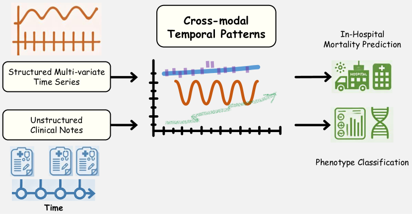
Figure 1: Motivation of our proposed CTPD: The core idea is to extract cross-modal temporal patterns (e.g., abnormal trends in blood pressure) to enhance the clinical outcome prediction from multimodal EHR data.

Existing approaches primarily address either the irregularity of data Shukla and Marlin (2019); Horn et al. (2020); Zhang et al. (2021, 2023) or the fusion of multiple modalities Huang et al. (2020); Zhang et al. (2020b); Xu et al. (2021); Kline et al. (2022), but they often neglect broader temporal trends that span across patient cases. These cross-modal temporal patterns, present in both structured and unstructured data, can provide high-level semantic insights into a patient’s health trajectory and potential risks Conrad et al. (2018). For instance, worsening trends in the vital signs of a patient, such as excessively high heart rate or blood pressure, may signal deteriorating health or a critical event, and these trends can also be reflected in clinical notes. Learning these global patterns in a cross-modal, temporal manner is expected to improve predictive performance. Furthermore, existing methods struggle to capture temporal patterns across varying time scales, which is critical for robust time series analysis.

To address these limitations, we propose the Cross-modal Temporal Pattern Discovery (CTPD) framework, designed to extract meaningful temporal patterns from multimodal EHR data to improve the accuracy of clinical outcome predictions. As shown in Fig. 1, the core innovation of our approach is a novel temporal pattern discovery module, which identifies corresponding temporal patterns (i.e., temporal prototypes) with meaningful semantics across both modalities throughout the dataset. This approach ensures that the model captures essential temporal semantics relevant to patient outcomes, providing a more comprehensive understanding of the data. To further enhance the quality of the learned temporal patterns, we introduce a InfoNCE Oord et al. (2018)-based TPNCE loss for aligning pattern embeddings across modalities, along with auxiliary reconstruction losses to ensure that the patterns retain core information of the data. Moreover, our framework incorporates a transformer Vaswani et al. (2017)-based fusion mechanism to effectively fuse the discovered temporal patterns with timestamp-level representations from both modalities, leading to more accurate predictions. We evaluate CTPD on two critical clinical prediction tasks: 48-hour in-hospital mortality prediction and 24-hour phenotype classification, using the MIMIC-III database. The results demonstrate the effectiveness of our approach, which significantly outperforms existing methods, and suggest a promising direction for improving multimodal EHR analysis for clinical prediction.

Contributions: (i). We propose a novel framework that captures cross-modal temporal patterns across multiple time scales in multimodal EHR data, offering a more comprehensive understanding of longitudinal patient information. (ii). Our framework incorporates a temporal pattern discovery module, utilizing slot attention to effectively extract meaningful semantic information. (iii). We introduce a TPNCE learning objective to optimize the temporal pattern discovery process, ensuring richer and more informative pattern learning. (iv). Our framework outperforms existing methods in two clinically critical tasks, demonstrating superior predictive performance.

2 Related Works

2.1 EHR Time-Series Data Analysis

EHR data is critical for clinical tasks such as disease diagnosis, mortality prediction, and treatment planning (Harutyunyan et al., 2019; Zhang et al., 2023). However, its high dimensionality and irregular nature pose challenges for traditional predictive models (Rani and Sikka, 2012; Lee et al., 2017). Deep learning models, such as RNNs and LSTMs, are often used to capture temporal dependencies in EHR data (Hayat et al., 2022; Deldari et al., 2023), but they struggle with irregular time intervals due to their reliance on fixed-length sequences (Xie et al., 2021). To address this, some methods update patient representations at each time step using graph neural networks (Zhang et al., 2021), while others employ time-aware embeddings to incorporate temporal information (Qian et al., 2023; Zhang et al., 2023). Despite these advancements, existing approaches still fail to capture high-level temporal patterns that are crucial for clinical outcomes. Subtle interactions between clinical parameters over extended periods—such as the relationship between blood pressure and creatinine levels—often hold the key to accurate predictions (Hanratty et al., 2011; Sun et al., 2024). Moreover, current methods struggle to model temporal patterns across varying time scales, limiting their effectiveness in clinical outcome predictions.

2.2 Prototype-based Pattern Learning

Prototype-based learning identifies representative instances (prototypes) and optimizes their distance from input data in latent space for tasks like classification (Li et al., 2023a; Ye et al., 2024). This approach has been widely applied in tasks such as anomaly detection, unsupervised learning, and few-shot learning (Tanwisuth et al., 2021; Li et al., 2023b). Recently, it has been extended to time-series data (Ghosal and Abbasi-Asl, 2021; Li et al., 2023a; Yu et al., 2024), demonstrating its potential for detecting complex temporal patterns. Additionally, prototype-based learning offers interpretable predictions, which is essential for healthcare applications (Zhang et al., 2024). However, learning efficient cross-modal temporal prototypes for multimodal EHR data remains an unexplored problem, as irregular time series and multi-scale patterns present significant challenges for existing methods.

2.3 Multi-modal Learning in Healthcare

In healthcare, patient data is typically collected in various forms—such as vital signs, laboratory results, medications, medical images, and clinical notes—to provide a comprehensive view of a patient’s health. Integrating these diverse modalities significantly enhances the performance of clinical tasks (Hayat et al., 2022; Zhang et al., 2023; Yao et al., 2024). However, fusing multimodal data remains challenging due to the heterogeneity and complexity of the sources. Earlier research on multimodal learning (Trong et al., 2020; Ding et al., 2022; Hayat et al., 2022) often rely on late fusion strategies, where unimodal representations are combined via concatenation or Kronecker products. While straightforward, these approaches often fail to capture complex inter-modal interactions, leading to suboptimal representations. Recent works have introduced transformer-based models that focus on cross-modal token interactions (Zhang et al., 2023; Theodorou et al., 2024; Yao et al., 2024). While these models are effective at capturing inter-modal relationships, they often struggle to extract high-level temporal semantics from multimodal data, limiting the ability to achieve a comprehensive understanding of a patient’s health conditions.

3 Methodology

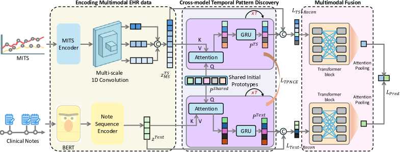
Figure 2: CTPD overview: the input Multivariate Irregular Time Series (MITS) and clinical note sequences are first encoded into regular embeddings. We then introduce the Cross-Modal Temporal Pattern Discovery module to extract meaningful temporal semantics. The extracted temporal patterns, along with the timestamp-level embeddings from both modalities, are fused to generate the final predictions.

We propose a novel temporal pattern discovery framework, as shown in Fig. 2, to uncover meaningful temporal patterns from multimodal EHR data, which we then leverage for clinical prediction tasks. In Section 3.1, we present the problem formulation. Section 3.2 outlines the encoding mechanisms for irregular time series and clinical notes. Following this, we introduce our proposed temporal pattern discovery mechanism in Section 3.3. Finally, the multimodal fusion mechanism and overall learning objectives are detailed in Section 3.4 and Section 3.5, respectively.

3.1 Problem Formulation

In practice, multimodal EHR datasets contain multiple data types, specifically Multivariate Irregular Time Series (MITS) and free-text clinical notes. We represent the multimodal EHR data for the $i$-th admission as $\{(\mathbf{x}_{(i)},\mathbf{t}^{\mathrm{TS}}_{(i)}),(n_{(i)},\mathbf{t}^{\mathrm{Text}}_{(i)}),\mathbf{y}_{(i)}\}_{i=1}^{N}$. Here $\mathbf{x}_{(i)}$ represents the multivariate time series observations, with $\mathbf{t}_{(i)}^{\mathrm{TS}}$ indicating their corresponding time points. The sequence of clinical notes is represented by $n_{(i)}$, and $\mathbf{t}_{(i)}^{\mathrm{Text}}$ denotes the time points of these notes. The variable $\mathbf{y}_{i}$ denotes the clinical outcomes to predict. For simplicity, we omit the admission index $i$ in subsequent sections. The MITS $\mathbf{x}$ comprises $d_{m}$ variables, where each variable $j=1,...,d_{m}$ has $l_{(j)}^{TS}$ observations, with the rest missing. Similarly, each clinical note sequence $n$ includes $l^{Text}$ notes. Early-stage medical prediction tasks aim to forecast an outcome $y$ for the admission $i$ using their multimodal EHR data $\{(\mathbf{x},\mathbf{t}^{\mathrm{TS}}),(n,\mathbf{t}^{\mathrm{Text}})\}$, specifically before a certain time point (e.g., 48 hours) after admission.

3.2 Encoding MITS and Clinical Notes

Here, we introduce our time series encoder $E_{\mathrm{TS}}$ and text encoder $E_{\mathrm{Text}}$, which separately encode MITS $(\mathbf{x},\mathbf{t}^{\mathrm{TS}})$ and clinical notes $(n,\mathbf{t}^{\mathrm{Text}})$ into their respective embeddings $\mathbf{z}^{\mathrm{TS}}$ and $\mathbf{z}^{\mathrm{Text}}\in\mathbb{R}^{T\times D}$. Here $T$ denotes the number of regular time points, and $D$ denotes the embedding dimension.

For MITS, we utilize a gating mechanism that dynamically integrates both irregular time series embeddings $\mathbf{e}_{\mathrm{imp}}^{\mathrm{TS}}$ and imputed regular time series embeddings $\mathbf{e}_{\mathrm{mTAND}}^{\mathrm{TS}}$, following the approach in Zhang et al. (2023). Formally, the MITS embedding $\mathbf{z}^{\mathrm{TS}}$ is computed as:

$$\mathbf{z}^{\mathrm{TS}}=\mathbf{g}\odot\mathbf{e}_{\mathrm{imp}}^{\mathrm{TS}}+(1-\mathbf{g})\odot\mathbf{e}_{\mathrm{mTAND}}^{\mathrm{TS}}$$ (1)

where $\mathbf{g}=f(\mathbf{e}_{\mathrm{imp}}^{\mathrm{TS}}\oplus\mathbf{e}_{\mathrm{mTAND}}^{\mathrm{TS}})$, $f(\cdot)$ is a gating function implemented via an MLP, $\oplus$ denotes the concatenation, and $\odot$ denotes point-wise multiplication.

The regular time series $\mathbf{e}_{\mathrm{imp}}^{\mathrm{TS}}$ embedding is derived by applying a 1D convolution layer to the imputed time series. At each reference time point $\alpha=1,...,T$, the imputed values are sourced from the nearest preceding values or replaced with a standard normal value if no prior data is available. Concurrently, mTAND (multi-time attention) Shukla and Marlin (2021) generates an alternative set of time series representations $\mathbf{e}_{\mathrm{mTAND}}^{\mathrm{TS}}$ with the same reference time points $\mathbf{r}$ with irregular time representations. Specifically, we leverage $V$ different Time2Vec Kazemi et al. (2019) functions $\{\theta_{v}(\cdot)\}_{v=1}^{V}$ to produce interpolation embeddings at each time point $\alpha$, which are then concatenated and linearly projected to form $\mathbf{e}_{\mathrm{mTAND}}^{\mathrm{TS}}(\alpha)\in\mathbb{R}^{D}$.

For clinical notes, embeddings are first extracted using Bert-tiny Turc et al. (2019); Bhargava et al. (2021), and another mTAND module is employed to generate embeddings $\mathbf{z}^{\mathrm{Text}}\in\mathbb{R}^{T\times D}$.

3.3 Discover Cross-modal Temporal Patterns from Multimodal EHR

High-level temporal patterns in multimodal EHR data often encode rich medical condition-related semantics that are crucial for predicting clinical outcomes. However, previous works primarily focus on timestamp-level embeddings, frequently overlooking these important temporal patterns (Bahadori and Lipton, 2019; Xiao et al., 2023; Sun et al., 2024). Drawing inspiration from object-centric learning in the computer vision domain (Locatello et al., 2020; Li et al., 2021), we propose a novel temporal pattern discovery module to capture complex patterns within longitudinal data.

Considering the hierarchical nature Yue et al. (2022); Cai et al. (2024) of time series data, the critical temporal patterns for EHR may manifest across multiple time scales. Consequently, our approach performs temporal pattern discovery on multi-scale time series embeddings.

Extracting Cross-modal Temporal Patterns. Owing to the correspondence within multi-modal data, our cross-modal temporal pattern discovery module focuses on extracting corresponding temporal patterns across both modalities for a better understanding of multimodal EHR. Starting with the time series embeddings $\mathbf{z}^{\mathrm{TS}}$ in Eq. 1, we generate multi-scale embeddings $\{\mathbf{z}^{\mathrm{TS}}_{(1)},\mathbf{z}^{\mathrm{TS}}_{(2)},\mathbf{z}^{\mathrm{TS}}_{(3)}\}$ using three convolutional blocks followed by mean pooling along the time dimension. The concatenated embedding $\mathbf{z}^{\mathrm{TS}}_{\mathrm{MS}}\in\mathbb{R}^{1.75T\times D}$ serves as the diverse temporal representation. We then enhance these embeddings by applying position encoding: $\mathbf{\hat{z}}^{\mathrm{TS}}_{\mathrm{MS}}=\mathbf{z}^{\mathrm{TS}}_{\mathrm{MS}}+\mathrm{PE}(\mathbf{z}^{\mathrm{TS}}_{\mathrm{MS}})$, $\mathbf{\hat{z}}^{\mathrm{TS}}_{\mathrm{MS}}\in\mathbb{R}^{1.75T\times D}$, where $\mathrm{PE}(\cdot)$ denotes the position embeddings in (Vaswani et al., 2017). Furthermore, to capture potential temporal patterns, we define a group of $K$ learnable vectors as temporal prototypes, $\mathbf{P}^{\mathrm{Shared}}\in\mathbb{R}^{K\times D}$, initially sampled from a normal distribution $\mathcal{N}(\mu,\operatorname{diag}(\sigma))\in\mathbb{R}^{K\times D}$ and refined during training. The shared prototype embeddings are designed to capture semantic-corresponding temporal patterns across modalities, respectively, with $\mu$ and $\sigma$ randomly initialized and subsequently optimized.

To extract temporal patterns, we first calculate the assignment weights $\mathbf{W}$ between prototype embeddings and modality embeddings using a dot-product attention mechanism:

$$\mathbf{W}^{\mathrm{TS}} =\mathrm{Attention}(\mathbf{P}^{\mathrm{Shared}},\mathbf{\hat{z}}^{\mathrm{TS}}_{\mathrm{MS}}),$$ (2)

$$\mathbf{W}^{\mathrm{Text}} =\mathrm{Attention}(\mathbf{P}^{\mathrm{Shared}},\mathbf{z}^{\mathrm{Text}})$$

The $\mathrm{Attention}$ mechanism is defined as:

$$\mathrm{Attention}(\mathbf{q},\mathbf{k})_{i,j} =\frac{e^{M_{i,j}}}{\sum_{l}e^{M_{i,l}}},$$ (3)

where $M=\frac{1}{\sqrt{D}}g_{q}(\mathbf{q})\cdot g_{k}(\mathbf{k})^{T}$ and $g_{q}(\cdot)$ and $g_{k}(\cdot)$ are two learnable matrices. Next, we aggregate the input values to their assigned prototypes using a weighted mean to obtain updated embeddings $\mathbf{z}^{\mathrm{TS}}_{\mathrm{updated}}$ and $\mathbf{z}^{\mathrm{Text}}_{\mathrm{updated}}$:

$$\mathbf{z}^{\mathrm{TS}}_{\mathrm{updated}} =\mathbf{W}^{\mathrm{TS}}\cdot v(\mathbf{\hat{z}}^{\mathrm{TS}}_{\mathrm{MS}})\in\mathbb{R}^{K\times D},$$ (4)

$$\mathbf{z}^{\mathrm{Text}}_{\mathrm{updated}} =\mathbf{W}^{\mathrm{Text}}\cdot v(\mathbf{\hat{z}}^{\mathrm{Text}})\in\mathbb{R}^{K\times D},$$

where $v(\cdot)$ is a learnable matrix.

Finally, the prototype embeddings $\mathbf{P}^{\mathrm{TS}}$ and $\mathbf{P}^{\mathrm{Text}}$ are refined using the corresponding updated embeddings via a learned recurrent function:

$$\mathbf{P}^{\mathrm{TS}} =f(\mathrm{GRU}(\mathbf{P}^{\mathrm{TS}}_{(0)}))\in\mathbb{R}^{K\times D}$$ (5)

$$\mathbf{P}^{\mathrm{Text}} =f(\mathrm{GRU}(\mathbf{P}^{\mathrm{Text}}_{(0)}))\in\mathbb{R}^{K\times D}$$

where $\mathbf{P}^{\mathrm{TS}}_{(0)}$ and $\mathbf{P}^{\mathrm{Text}}_{(0)}$ are the prototype embeddings from the previous step , $\mathrm{GRU}(\cdot)$ is Gated Recurrent Unit (Cho et al., 2014), and $f(\cdot)$ denotes MLP. The above process is repeated for 3 iterations per step. Those refined embeddings denote the discovered temporal patterns for each modality.

TPNCE Contraint. To ensure consistent semantics across modalities, we introduce a TPNCE loss, inspired by InfoNCE Oord et al. (2018), to enforce the similarity of multimodal prototype embeddings for the same admission while increasing the distance between prototype embeddings from different admissions. For a minibatch of $B$ samples, the TPNCE loss from MITS to notes is defined as:

$$\mathcal{L}_{\mathrm{TPNCE}}^{\mathrm{TS}\rightarrow\mathrm{Text}}=-\sum_{i=1}^{B}\big{(}\mathrm{log}\frac{\mathrm{exp}(\mathrm{sim}(i,i)/\tau)}{\sum_{j=1}^{B}\mathrm{exp}(\mathrm{sim}(i,j)/\tau)}\big{)}$$ (6)

where $\tau$ is a temperature parameter. The bidirectional TPNCE loss is then given by:

$$\mathcal{L}_{\mathrm{TPNCE}}=\frac{1}{2}(\mathcal{L}_{\mathrm{TPNCE}}^{\mathrm{TS}\rightarrow\mathrm{Text}}+\mathcal{L}_{\mathrm{TPNCE}}^{\mathrm{Text}\rightarrow\mathrm{TS}})$$ (7)

The similarity function $\mathrm{sim}(i,j)$ measures the similarity between the $i$-th $\mathbf{P}^{\mathrm{TS}}$ and $j$-th $\mathbf{P}^{\mathrm{Text}}$, and is defined as (for convenience, we omit the indices $i$ and $j$ in the equation below):

$${\mathrm{sim}(\cdot)=\sum_{k=1}^{K}(\beta_{k}<\mathbf{P}^{\mathrm{TS}}(k),\mathbf{P}^{\mathrm{Text}}(k)>)}$$ (8)

where $\langle\cdot\rangle$ denotes cosine similarity, and $k$ is the prototype index. To account for varying prototype importance, an attention mechanism is used to generate weights $\mathbf{\beta}$ for the slots, based on global MITS and text embeddings: $\mathbf{\beta}=\mathrm{MLP}(\mathrm{concat}[\mathbf{g}^{\mathrm{TS}}_{\mathrm{MS}},\mathbf{g}^{\mathrm{Text}}])$, where $\mathbf{g}^{\mathrm{TS}}_{\mathrm{MS}}$ and $\mathbf{g}^{\mathrm{Text}}\in\mathbb{R}^{D}$ are global embeddings obtained by averaging $\mathbf{\hat{z}}^{\mathrm{TS}}_{\mathrm{MS}}$ and $\mathbf{z}^{\mathrm{Text}}$ along the time dimension.

Auxiliary Reconstruction. To ensure that the learned prototype representations capture core information from multimodal EHR data, we introduce two reconstruction objectives aimed at reconstructing imputed regular time series and text embeddings from the learned prototypes. Specifically, we implement a time series decoder to reconstruct the imputed regular time series from $\mathbf{P}^{\mathrm{TS}}$, and a text embedding decoder to reconstruct text embeddings from $\mathbf{P}^{\mathrm{Text}}$. Both decoders are based on a transformer decoder architecture Vaswani et al. (2017), and two mean squared error (MSE) losses denoted by $\mathcal{L}_{\mathrm{TS-Recon}}$ and $\mathcal{L}_{\mathrm{Text-Recon}}$ are used as the objective function. Here, we define the overall reconstruction loss $\mathcal{L}_{\mathrm{Recon}}=\frac{1}{2}(\mathcal{L}_{\mathrm{TS-Recon}}+\mathcal{L}_{\mathrm{Text-Recon}})$.

3.4 Multimodal Fusion

In practice, medical conditions are influenced by both timestamp-level embeddings and high-level temporal patterns. So our prediction is made by integrating both types of information for comprehensive analysis. Since information from both modalities is crucial for predicting medical conditions, we propose a multimodal fusion mechanism to integrate these inputs. First, we apply a 2-layer transformer encoder Vaswani et al. (2017) to learn interactions across all embeddings from both modalities. Then, we aggregate embeddings of each modality using an attention-based pooling mechanism:

$$\mathbf{F}^{\mathrm{TS}} =\sum_{k=1}^{K}\mathbf{\gamma}_{k}^{\mathrm{TS}}\mathbf{P}^{\mathrm{TS}}(k)+\sum_{t=1}^{T}\mathbf{\phi}_{t}^{\mathrm{TS}}\hat{\mathbf{z}}^{\mathrm{TS}}_{\mathrm{MS}}(t)$$ (9)

$$\mathbf{F}^{\mathrm{Text}} =\sum_{k=1}^{K}\mathbf{\gamma}_{k}^{\mathrm{Text}}\mathbf{P}^{\mathrm{Text}}(k)+\sum_{t=1}^{T}\mathbf{\phi}_{t}^{\mathrm{Text}}\mathbf{z}^{\mathrm{Text}}_{\mathrm{Text}}(t)$$

Here $\mathbf{\gamma}^{\mathrm{TS}}$, $\mathbf{\phi}^{\mathrm{TS}}$, $\mathbf{\gamma}^{\mathrm{Text}}$, $\mathbf{\phi}^{\mathrm{Text}}$ are learned attention weights. The resulting global embeddings from both modalities are concatenated along the feature dimension to form the final global representation.

3.5 Overall Learning Objectives

To optimize our framework, we employ four loss functions jointly. The primary loss, $\mathcal{L}_{\mathrm{pred}}$, is a cross-entropy loss used for classification. Next, the TPNCE loss, $\mathcal{L}_{\mathrm{TPNCE}}$, enforces consistency between prototype embeddings across modalities. Additionally, the reconstruction loss $\mathcal{L}_{\mathrm{Recon}}$ ensures that the extracted temporal patterns capture sufficient information from samples. The overall objective is a weighted sum of these loss functions:

$$\mathcal{L}= \mathcal{L}_{\mathrm{pred}}+\lambda_{1}*\mathcal{L}_{\mathrm{TPNCE}}+\lambda_{2}*\mathcal{L}_{\mathrm{Recon}}$$ (10)

where $\lambda_{1}$, $\lambda_{2}$ are hyperparameters that control the weights of respective losses.

Table 1: Number of samples for two evaluation tasks.

	48-IHM			24-PHE
	Total	Positive	Negative	Total
Training	15425	2011	13414	25435
Validation	1727	245	1482	2807
Test	3107	359	2748	5013

Table 2: Comparison of our method with baselines on 48-IHM and 24-PHE tasks using the MIMIC-III dataset. We report average performance on three random seeds, with standard deviation as the subscript. The Best and 2nd best methods under each setup are bold and underlined.

Model	48-IHM			24-PHE
	AUROC ($\uparrow$)	AUPR ($\uparrow$)	F1 ($\uparrow$)	AUROC ($\uparrow$)	AUPR ($\uparrow$)	F1 ($\uparrow$)
Methods on MITS.
CNN (LeCun et al., 1998)	85.80${}_{\textit{0.32}}$	49.73${}_{\textit{0.65}}$	46.37${}_{\textit{3.01}}$	75.36${}_{\textit{0.18}}$	38.10${}_{\textit{0.26}}$	40.80${}_{\textit{0.37}}$
RNN (Elman, 1990)	84.75${}_{\textit{0.74}}$	46.57${}_{\textit{1.18}}$	45.60${}_{\textit{2.06}}$	73.78${}_{\textit{0.10}}$	36.76${}_{\textit{0.27}}$	33.99${}_{\textit{0.48}}$
LSTM Hochreiter (1997)	85.22${}_{\textit{0.67}}$	46.93${}_{\textit{1.28}}$	45.72${}_{\textit{1.41}}$	74.46${}_{\textit{0.23}}$	36.80${}_{\textit{0.28}}$	39.45${}_{\textit{0.49}}$
Transformer (Vaswani et al., 2017)	83.45${}_{\textit{0.97}}$	43.03${}_{\textit{1.65}}$	39.31${}_{\textit{3.83}}$	74.98${}_{\textit{0.14}}$	39.37${}_{\textit{0.26}}$	36.13${}_{\textit{1.42}}$
IP-Net (Shukla and Marlin, 2019)	81.76${}_{\textit{0.38}}$	39.50${}_{\textit{0.83}}$	43.89${}_{\textit{1.07}}$	73.98${}_{\textit{0.13}}$	35.31${}_{\textit{0.29}}$	39.38${}_{\textit{0.15}}$
GRU-D (Che et al., 2018)	49.21${}_{\textit{5.26}}$	12.85${}_{\textit{2.24}}$	19.63${}_{\textit{0.01}}$	52.11${}_{\textit{0.42}}$	17.99${}_{\textit{0.55}}$	26.17${}_{\textit{0.23}}$
DGM-O (Wu et al., 2021)	71.99${}_{\textit{7.30}}$	28.67${}_{\textit{7.34}}$	31.72${}_{\textit{11.02}}$	60.70${}_{\textit{0.82}}$	22.56${}_{\textit{0.77}}$	28.87${}_{\textit{0.64}}$
mTAND (Shukla and Marlin, 2021)	85.27${}_{\textit{0.20}}$	49.82${}_{\textit{0.97}}$	48.02${}_{\textit{1.93}}$	72.79${}_{\textit{0.09}}$	35.95${}_{\textit{0.14}}$	32.42${}_{\textit{0.72}}$
SeFT (Horn et al., 2020)	65.00${}_{\textit{0.84}}$	22.93${}_{\textit{1.27}}$	19.70${}_{\textit{15.59}}$	60.50${}_{\textit{0.09}}$	23.57${}_{\textit{0.07}}$	21.26${}_{\textit{0.21}}$
UTDE (Zhang et al., 2023)	86.14${}_{\textit{0.45}}$	50.60${}_{\textit{0.28}}$	49.29${}_{\textit{0.62}}$	73.62${}_{\textit{0.57}}$	36.80${}_{\textit{0.87}}$	40.58${}_{\textit{0.64}}$
Methods on Clinical Notes.
Flat Deznabi et al. (2021)	85.71${}_{\textit{0.49}}$	50.96${}_{\textit{0.19}}$	45.80${}_{\textit{6.61}}$	81.77${}_{\textit{0.09}}$	53.79${}_{\textit{0.21}}$	52.13${}_{\textit{0.79}}$
HierTrans Pappagari et al. (2019)	84.32${}_{\textit{0.34}}$	47.92${}_{\textit{0.57}}$	42.01${}_{\textit{0.58}}$	80.79${}_{\textit{0.06}}$	51.97${}_{\textit{0.08}}$	50.85${}_{\textit{0.71}}$
T-LSTM Baytas et al. (2017)	85.70${}_{\textit{0.21}}$	45.29${}_{\textit{0.86}}$	42.84${}_{\textit{5.53}}$	81.15${}_{\textit{0.04}}$	50.23${}_{\textit{0.07}}$	49.77${}_{\textit{0.24}}$
FT-LSTM Zhang et al. (2020a)	84.28${}_{\textit{0.95}}$	43.93${}_{\textit{1.03}}$	36.87${}_{\textit{6.54}}$	81.66${}_{\textit{0.12}}$	51.71${}_{\textit{0.24}}$	50.21${}_{\textit{0.85}}$
GRU-D (Che et al., 2018)	72.58${}_{\textit{0.42}}$	26.38${}_{\textit{1.06}}$	31.64${}_{\textit{0.79}}$	49.52${}_{\textit{0.65}}$	16.90${}_{\textit{0.12}}$	27.80${}_{\textit{0.08}}$
mTAND (Shukla and Marlin, 2021)	85.40${}_{\textit{0.60}}$	49.68${}_{\textit{1.26}}$	35.76${}_{\textit{11.57}}$	82.14${}_{\textit{0.07}}$	54.57${}_{\textit{0.15}}$	52.01${}_{\textit{0.93}}$
Methods on Multimodal EHR.
MMTM (Joze et al., 2020)	87.88${}_{\textit{0.07}}$	53.58${}_{\textit{0.24}}$	51.54${}_{\textit{1.58}}$	81.46${}_{\textit{0.25}}$	51.88${}_{\textit{0.12}}$	51.59${}_{\textit{0.19}}$
DAFT (Pölsterl et al., 2021)	87.53${}_{\textit{0.22}}$	52.40${}_{\textit{0.21}}$	51.95${}_{\textit{0.64}}$	81.18${}_{\textit{0.08}}$	50.91${}_{\textit{0.31}}$	50.72${}_{\textit{0.39}}$
MedFuse (Hayat et al., 2022)	86.02${}_{\textit{0.29}}$	51.00${}_{\textit{0.22}}$	49.29${}_{\textit{0.75}}$	78.88${}_{\textit{0.14}}$	45.99${}_{\textit{0.21}}$	47.47${}_{\textit{0.23}}$
DrFuse (Yao et al., 2024)	85.97${}_{\textit{1.02}}$	49.94${}_{\textit{1.91}}$	49.75${}_{\textit{1.52}}$	80.88${}_{\textit{0.18}}$	49.62${}_{\textit{0.40}}$	50.18${}_{\textit{0.31}}$
CTPD (Ours)	88.15${}_{\textit{0.28}}$	53.86${}_{\textit{0.65}}$	53.85${}_{\textit{0.16}}$	83.34${}_{\textit{0.05}}$	56.39${}_{\textit{0.17}}$	53.83${}_{\textit{0.43}}$

Table 3: Ablation results show the impact of removing different types of input embeddings.

	48-IHM			24-PHE
	AUROC	AUPR	F1	AUROC	AUPR	F1
Ours	88.15${}_{\textit{0.28}}$	53.86${}_{\textit{0.65}}$	53.85${}_{\textit{0.16}}$	83.34${}_{\textit{0.05}}$	56.39${}_{\textit{0.17}}$	53.83${}_{\textit{0.43}}$
:w/o prototype	86.89${}_{\textit{0.97}}$	53.67${}_{\textit{0.65}}$	48.47${}_{\textit{6.13}}$	82.24${}_{\textit{0.07}}$	54.06${}_{\textit{0.07}}$	52.88${}_{\textit{0.11}}$
:w/o timestamp embeddings	87.18${}_{\textit{0.94}}$	54.32${}_{\textit{1.66}}$	45.85${}_{\textit{4.91}}$	82.41${}_{\textit{0.15}}$	54.30${}_{\textit{0.21}}$	53.34${}_{\textit{0.41}}$
:w/o multi-scale embedding	87.59${}_{\textit{0.49}}$	53.38${}_{\textit{1.79}}$	49.74${}_{\textit{3.50}}$	83.11${}_{\textit{0.09}}$	55.95${}_{\textit{0.05}}$	53.81${}_{\textit{0.46}}$

Table 4: Ablation study of loss functions $\mathcal{L}_{\mathrm{TPNCE}}$ and $\mathcal{L}_{\mathrm{Recon}}$. The Best results are highlighted in bold.

		48-IHM			24-PHE
Cont	Recon	AUROC	AUPR	F1	AUROC	AUPR	F1
		87.49${}_{\textit{0.47}}$	53.31${}_{\textit{1.46}}$	43.59${}_{\textit{4.63}}$	82.49${}_{\textit{0.10}}$	55.25${}_{\textit{0.30}}$	53.71${}_{\textit{0.43}}$
✓		87.15${}_{\textit{0.38}}$	53.45${}_{\textit{1.09}}$	44.76${}_{\textit{4.48}}$	82.94${}_{\textit{0.05}}$	55.62${}_{\textit{0.22}}$	53.99${}_{\textit{0.19}}$
	✓	86.93${}_{\textit{0.69}}$	52.70${}_{\textit{1.97}}$	41.52${}_{\textit{0.90}}$	82.86${}_{\textit{0.03}}$	55.43${}_{\textit{0.05}}$	54.08${}_{\textit{0.29}}$
✓	✓	88.15${}_{\textit{0.28}}$	53.86${}_{\textit{0.65}}$	53.85${}_{\textit{0.16}}$	83.34${}_{\textit{0.05}}$	56.39${}_{\textit{0.17}}$	53.83${}_{\textit{0.43}}$

4 Experiment

4.1 Experimental Setup

Dataset. We assess our model’s efficacy using MIMIC-III v1.4, a comprehensive open-source multimodal clinical database (Johnson et al., 2023). We focus our evaluation on two critical tasks, 48-hour in-hospital mortality prediction (48-IHM) and 24-hour phenotype classification (24-PHE), as established in prior research (Zhang et al., 2023). Following the data preprocessing pipeline from (Harutyunyan et al., 2019), we extract $17$ clinical variables from the numerical time series. Following the dataset splitting by (Harutyunyan et al., 2019), we ensure that the model evaluation is robust by partitioning the data into $70\%$ training, $10\%$ validation, and $20\%$ testing sets, based on unique subject IDs to prevent information leakage. The specific dataset statistics are shown in Table 1.

Evaluation Metrics. The 48-hour In-Hospital Mortality (48-IHM) prediction is a binary classification with a marked label imbalance, indicated by a death-to-discharge ratio of approximately 1:6. Following previous work (Harutyunyan et al., 2019; Zhang et al., 2023), we use AUROC, AUPR, and F1 score, for a comprehensive evaluation. The $24$-hour Phenotype Classification (24-PHE) involves predicting the presence of 25 different medical conditions during an ICU stay, making it a multi-label classification task. For this task, we employ the AUROC, AUPR, and F1 score (Macro) for a thorough assessment of model efficacy. The F1 score threshold is determined by selecting the value that maximizes the F1 score on the validation set.

Implementation Details. Preprocessing pipeline of MIST follows Harutyunyan et al. (2019), and the clinical note preprocessing pipeline follows Khadanga et al. (2019). We train the model with batch size of 128, learning rate of 4e-5, and Adam (Kingma and Ba, 2014) optimizer. We use a cosine annealing learning rate scheduler with a 0.2 warm-up proportion. To prevent overfitting, we implement early stopping when there is no increase in the AUROC on the validation set for 48-IHM or 24-PHENO over $5$ consecutive epochs. All experiments are conducted on 1 RTX-3090 GPU card using about 1 hour per run. We clip the norm of gradient values with 0.5 for stable training. By default, we use Bert-tiny Turc et al. (2019); Bhargava et al. (2021) as our text encoder.

Compared Methods. To ensure a comprehensive comparison, we compare our CTPD with three types baselines: MITS-only approaches, note-only approaches and multimodal approaches. For MITS-only setting, we compare CTPD with 4 baselines for imputed regular time series: RNN (Elman, 1990), LSTM (Hochreiter, 1997), CNN (LeCun et al., 1998) and Transformer Vaswani et al. (2017), and 5 baselines for irregular time series, including IP-Net (Shukla and Marlin, 2019), GRU-D (Che et al., 2018), DGM-O (Wu et al., 2021), mTAND (Shukla and Marlin, 2021), SeFT (Horn et al., 2020), and UTDE (Zhang et al., 2023). The imputation approach follows the MIMIC-III benchmark (Harutyunyan et al., 2019). For the note-only setting, we compare our model with 6 baselines: Flat Deznabi et al. (2021), HierTrans Pappagari et al. (2019), T-LSTM Baytas et al. (2017), FT-LSTM Zhang et al. (2020a), GRU-D (Che et al., 2018), and mTAND (Shukla and Marlin, 2021). In the multimodal setting, we compare our model with 4 baselines: MMTM Joze et al. (2020), DAFT Pölsterl et al. (2021), MedFuse Hayat et al. (2022), and DrFuse Yao et al. (2024). To ensure a fair comparison, we implement Bert-tiny Bhargava et al. (2021); Turc et al. (2019) as the text encoder across all baselines. Details of baselines can be found in the Appendix B.

4.2 Comparison with SOTA Baselines

Table 2 presents a comparison of our proposed CTPD against three types of baselines: MITS-based methods, clinical notes-based methods, and multimodal EHR-based methods. Our CTPD, which incorporates both timestamp-level embeddings and temporal pattern embeddings from multimodal data, consistently achieves the best performance across two tasks on all three different metrics. Specifically, CTPD shows a $1.89\%$ improvement in F1 score on the 48-IHM task, and a $1.2\%$ improvement in AUROC and $1.92\%$ in AUPR on the more challenging 24-PHE task, compared to the second-best results. Note that the standard deviation of our approach is relatively small, which further validates the significant improvements we have achieved compared with baselines. Overall, CTPD outperforms all baselines considered in this paper across two clinical tasks over three metrics, demonstrating its effectiveness in extracting cross-modal temporal patterns to enhance clinical outcome prediction.

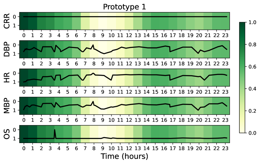
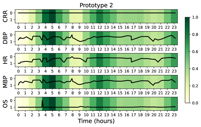
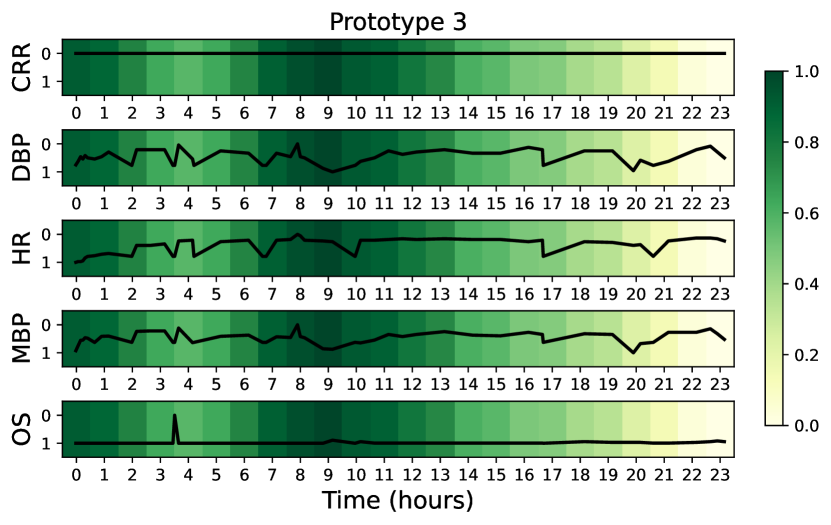
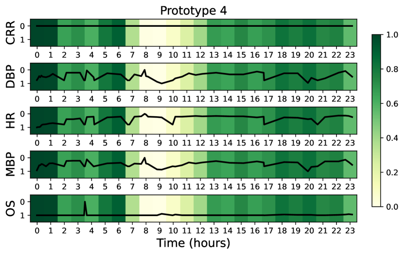
Figure 3: Visualization of the learned prototypes in our CTPD framework. Here we select $5$ representative clinical variables to visualize the time series. “DBP" denotes “Diastolic blood pressure", “G" denotes “Glucose", “HR" denotes “Heart Rate", “MBP" denotes “Mean blood pressure" and “OS" denotes “Oxygen saturation".

4.3 Model Analysis

Ablation Results on Different Types of Embeddings. We conduct ablation studies by removing the prototype embeddings, timestamp-level embeddings, and multi-scale feature extractor respectively, and analyze their impacts on two clinical prediction tasks, as shown in Table 3. Notably, prototype embeddings play the most significant role among the three components, with their removal resulting in a $1.96\%$ AUROC decrease in 48-IHM and a $1.1\%$ decrease in 24-PHE. The results also show that all three embeddings are important for capturing effective information for prediction.

Ablation Results on Learning Objectives. Table 4 presents the ablation results of the learning objectives. Combining both $\mathcal{L}_{\mathrm{TPNCE}}$ and $\mathcal{L}_{\mathrm{Recon}}$ leads to the best performance across 5 out of 6 settings. Our model is also relatively robust to different loss function configurations, with only a $0.66\%$ AUROC drop in the model’s performance in 48-IHM and a $0.85\%$ drop in 24-IHM.

Ablation Results on Hyperparameters. We analyze the effects of two key hyperparameters: loss weights $\lambda_{1}$ and $\lambda_{2}$, shown in Table 5, and the number of prototypes in Fig. 4. For the loss weights, $\lambda_{1}=0.1$ and $\lambda_{2}=0.5$ consistently yield the best performance across all settings. However, excessively large values for $\lambda_{1}$ and $\lambda_{2}$ can cause the model to prioritize cross-modal alignment and reconstruction tasks over predictive performance. Regarding the number of prototypes, we find that using 16 prototypes achieves the best results, though our model remains robust, with 8 prototypes yielding similar outcomes.

Table 5: Ablation results on loss weights. The parameters $\lambda_{1}$ and $\lambda_{2}$ control the strength of the $\mathcal{L}_{\mathrm{TPNCE}}$ and $\mathcal{L}_{\mathrm{Recon}}$ losses, respectively.

$\lambda_{1}$	$\lambda_{2}$	48-IHM			24-PHE
		AUROC	AUPR	F1	AUROC	AUPR	F1
0.1	0.1	87.21${}_{\textit{0.36}}$	53.80${}_{\textit{0.28}}$	47.41${}_{\textit{9.17}}$	82.93${}_{\textit{0.05}}$	55.62${}_{\textit{0.22}}$	54.00${}_{\textit{0.20}}$
0.1	0.5	88.15${}_{\textit{0.28}}$	53.86${}_{\textit{0.65}}$	53.85${}_{\textit{0.16}}$	83.34${}_{\textit{0.05}}$	56.39${}_{\textit{0.17}}$	53.83${}_{\textit{0.43}}$
0.5	0.5	87.20${}_{\textit{0.47}}$	53.77${}_{\textit{0.47}}$	42.44${}_{\textit{7.45}}$	82.59${}_{\textit{0.09}}$	55.22${}_{\textit{0.04}}$	53.42${}_{\textit{0.04}}$
1	0.5	86.59${}_{\textit{2.19}}$	51.93${}_{\textit{5.31}}$	47.93${}_{\textit{3.13}}$	82.44${}_{\textit{0.03}}$	54.84${}_{\textit{0.18}}$	53.29${}_{\textit{0.29}}$
1	1	86.64${}_{\textit{2.10}}$	52.34${}_{\textit{5.79}}$	50.09${}_{\textit{4.34}}$	82.54${}_{\textit{0.48}}$	55.03${}_{\textit{0.39}}$	53.94${}_{\textit{1.31}}$
1	2	85.56${}_{\textit{1.19}}$	50.66${}_{\textit{4.17}}$	44.67${}_{\textit{3.88}}$	76.88${}_{\textit{1.84}}$	41.89${}_{\textit{3.05}}$	44.83${}_{\textit{2.31}}$

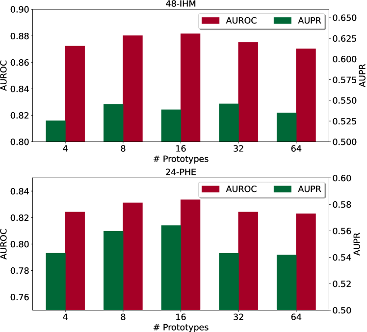
Figure 4: Ablation study on the number of prototypes.

4.4 Qualitative Results

Fig. 3 shows a case study of our model. We randomly select 16 prototypes to visualize cross-modal temporal patterns. It verifies that our model can extract different types of temporal patterns from the multimodal EHR. We will further explore interpreting these prototypes using LLM for more clinical insights.

5 Conclusion

In this paper, we present the Cross-Modal Temporal Pattern Discovery (CTPD) framework, which captures cross-modal temporal patterns and incorporates them with timestamp-level embeddings for more accurate clinical outcome predictions based on multimodal EHR data. To efficiently optimize the framework, we introduce a contrastive-based TPNCE loss to enhance cross-modal alignment, along with two reconstruction objectives to retain core information from each modality. Our experiments on two clinical prediction tasks using the MIMIC-III dataset demonstrate the effectiveness of CTPD in multimodal EHR analysis.

6 Limitations

Our framework relies on datasets with paired time series and clinical notes to learn similar semantic patterns from both modalities. However, in practice, datasets with missing modalities are more common, and our current framework does not easily adapt to scenarios with missing data modalities. Additionally, learning efficient temporal patterns from unpaired multimodal datasets remains a challenge. Another limitation of our approach is that it primarily extracts temporal semantics in the embedding space, which limits the model’s interpretability. While our method effectively captures temporal patterns, it offers limited insights into the detailed relationships between data from different modalities. Finally, our framework is currently designed for specific clinical prediction tasks. In practice, there are various prediction tasks related to multimodal EHR analysis. Extending the proposed method into a more generalized or foundational model capable of handling multiple downstream tasks with minimal training annotations could be more practical and effective. Our future work will focus on resolving those aspects.

Potential Risks. The medical dataset used in our framework must be carefully reviewed to mitigate any potential identification risk. Additionally, our framework is developed solely for research purposes and is not intended for commercial use. Note that AI assistant was used only for polishing the writing of this paper.

Appendix

Appendix A Additional Information on Datasets

The 17 variables from the MIMIC-III dataset that we use include 5 categorical variables (capillary refill rate, Glasgow coma scale eye opening, Glasgow coma scale motor response, Glasgow coma scale total, and Glasgow coma scale verbal response) and 12 continuous measures (diastolic blood pressure, fraction of inspired oxygen, glucose, heart rate, height, mean blood pressure, oxygen saturation, respiratory rate, systolic blood pressure, temperature, weight, and pH).

Appendix B More Details on Baselines

Baselines only using MITS

• CNN (LeCun et al., 1998): CNN (Convolutional Neural Network) uses backpropagation to synthesize a complex decision surface that facilitates learning.

• RNN (Elman, 1990): RNN (Residual Neural Network) is trained to process data sequentially so as to model the time dimension of data.

• LSTM Hochreiter (1997): LSTM (Long short-term memory) is a variant of recurrent neural network. It excels at dealing with the vanishing gradient problem and is relatively insensitive to time gap length.

• Transformer (Vaswani et al., 2017): Transformer is a powerful deep learning architecture based on attention mechanism. It has great generalisability and has been adopted as foundation model in multiple research domains.

• IP-Net (Shukla and Marlin, 2019): IP-Net (Interpolation-Prediction Network) is a deep learning architecture for supervised learning focusing on processing sparse multivariate time series data that are sampled irregularly.

• GRU-D (Che et al., 2018): GRU-D is based on GRU (Gated Recurrent Unit). It incorporates features of missing data in EHR into the model architecture to improve prediction results.

• DGM-O (Wu et al., 2021): DGM-O (Dynamic Gaussian Mixture based Deep Generative Model) is a generative model derived from a dynamic Gaussian mixture distribution. It makes predictions based on incomplete inputs. DGM-O is instantiated with multilayer perceptron (MLP).

• mTAND (Shukla and Marlin, 2021): mTAND (Multi-Time Attention network) is a deep learning model that learns representations of continuous time values and uses an attention mechanism to generate a consistent representation of a time series based on a varying amount of observations.

• SeFT (Horn et al., 2020): SeFT (Set Functions for Time Series) addresses irregularly-sampled time series. It is based on differentiable set function learning.

• UTDE (Zhang et al., 2023): UTDE (Unified TDE module) is built upon TDE (Temporal discretization-based embedding). It models asynchronous time series data by combining imputation embeddings and learned interpolation embeddings through a gating mechanism. It also uses a time attention mechanism.

Baselines only using clinical notes

• Flat Deznabi et al. (2021): Flat encodes clinical notes using a fine-tuned BERT model. It also utilizes an LSTM model that takes in patients’ vital signals so as to jointly model the two modalities. Furthermore, it addresses the temporal irregularity issue of modeling patients’ vital signals.

• HierTrans Pappagari et al. (2019): HierTrans (Hierarchical Transformers) is built upon BERT model. It achieves an enhanced ability to take in long inputs by first partitioning the inputs into shorter sequences and processing them separately. Then, it propagates each output via a recurrent layer.

• T-LSTM Baytas et al. (2017): T-LSTM (Time-Aware LSTM) deals with irregular time intervals in EHRs by learning decomposed cell memory which models elapsed time. The final patient subtyping model uses T-LSTM in an auto-encoder module before doing patient subtyping.

• FT-LSTM Zhang et al. (2020a): FT-LSTM (Flexible Time-aware LSTM Transformer) models the multi-level structure in clinical notes. At the base level, it uses a pre-trained ClinicalBERT model. Then, it merges sequential information and content embedding into a new position-enhanced representation. Then, it uses a time-aware layer that considers the irregularity of time intervals.

• GRU-D (Che et al., 2018): Please refer to the above subsection.

• mTAND (Shukla and Marlin, 2021): Please refer to the above subsection.

Baselines using multimodal EHR

• MMTM (Joze et al., 2020): MMTM (Multi-modal Transfer Module) is a neural network module that leverages knowledge from various modalities in CNN. It can recalibrate features in each CNN stream via excitation and squeeze operations.

• DAFT (Pölsterl et al., 2021): DAFT (Dynamic Affine Feature Map Transform) is a general-purpose CNN module that alters the feature maps of a convolutional layer with respect to a patient’s clinical data.

• MedFuse (Hayat et al., 2022): MedFuse is an LSTM-based fusion module capable of processing both uni-modal and multi-modal input. It treats multi-modal representations of data as a sequence of uni-modal representations. It handles inputs of various lengths via the recurrent inductive bias of LSTM.

• DrFuse (Yao et al., 2024): DrFuse is a fusion module that addresses the issue of missing modality by separating the unique features within each modality and the common ones across modalities. It also adds a disease-wise attention layer for each modality.

References

- Acosta et al. (2022) Julián N. Acosta, Guido J. Falcone1, Pranav Rajpurka, and Eric J. Topol. 2022. Multimodal biomedical AI. Nature Medicine, 28:1773–1784.
- Bahadori and Lipton (2019) Mohammad Taha Bahadori and Zachary Chase Lipton. 2019. Temporal-clustering invariance in irregular healthcare time series. arXiv preprint arXiv:1904.12206.
- Baytas et al. (2017) Inci M Baytas, Cao Xiao, Xi Zhang, Fei Wang, Anil K Jain, and Jiayu Zhou. 2017. Patient subtyping via time-aware lstm networks. In Proceedings of the 23rd ACM SIGKDD international conference on knowledge discovery and data mining, pages 65–74.
- Bhargava et al. (2021) Prajjwal Bhargava, Aleksandr Drozd, and Anna Rogers. 2021. Generalization in nli: Ways (not) to go beyond simple heuristics. Preprint, arXiv:2110.01518.
- Cai et al. (2024) Wanlin Cai, Yuxuan Liang, Xianggen Liu, Jianshuai Feng, and Yuankai Wu. 2024. Msgnet: Learning multi-scale inter-series correlations for multivariate time series forecasting. In Proceedings of the AAAI Conference on Artificial Intelligence, volume 38, pages 11141–11149.
- Che et al. (2018) Zhengping Che, Sanjay Purushotham, Kyunghyun Cho, David Sontag, and Yan Liu. 2018. Recurrent neural networks for multivariate time series with missing values. Scientific reports, 8(1):6085.
- Cho et al. (2014) Kyunghyun Cho, Bart Van Merriënboer, Caglar Gulcehre, Dzmitry Bahdanau, Fethi Bougares, Holger Schwenk, and Yoshua Bengio. 2014. Learning phrase representations using rnn encoder-decoder for statistical machine translation. arXiv preprint arXiv:1406.1078.
- Conrad et al. (2018) Nathalie Conrad, Andrew Judge, Jenny Tran, Hamid Mohseni, Deborah Hedgecott, Abel Perez Crespillo, Moira Allison, Harry Hemingway, John G Cleland, John JV McMurray, et al. 2018. Temporal trends and patterns in heart failure incidence: a population-based study of 4 million individuals. The Lancet, 391(10120):572–580.
- Deldari et al. (2023) Shohreh Deldari, Dimitris Spathis, Mohammad Malekzadeh, Fahim Kawsar, Flora Salim, and Akhil Mathur. 2023. Latent masking for multimodal self-supervised learning in health timeseries. arXiv preprint arXiv:2307.16847.
- Deznabi et al. (2021) Iman Deznabi, Mohit Iyyer, and Madalina Fiterau. 2021. Predicting in-hospital mortality by combining clinical notes with time-series data. In Findings of the association for computational linguistics: ACL-IJCNLP 2021, pages 4026–4031.
- Ding et al. (2022) Ning Ding, Sheng-wei Tian, and Long Yu. 2022. A multimodal fusion method for sarcasm detection based on late fusion. Multimedia Tools and Applications, 81(6):8597–8616.
- Elman (1990) Jeffrey L Elman. 1990. Finding structure in time. Cognitive science, 14(2):179–211.
- Ghosal and Abbasi-Asl (2021) Gaurav R Ghosal and Reza Abbasi-Asl. 2021. Multi-modal prototype learning for interpretable multivariable time series classification. arXiv preprint arXiv:2106.09636.
- Hanratty et al. (2011) Rebecca Hanratty, Michel Chonchol, Edward P Havranek, J David Powers, L Miriam Dickinson, P Michael Ho, David J Magid, and John F Steiner. 2011. Relationship between blood pressure and incident chronic kidney disease in hypertensive patients. Clinical journal of the American Society of Nephrology: CJASN, 6(11):2605.
- Harutyunyan et al. (2019) Hrayr Harutyunyan, Hrant Khachatrian, David C Kale, Greg Ver Steeg, and Aram Galstyan. 2019. Multitask learning and benchmarking with clinical time series data. Scientific data, 6(1):96.
- Hayat et al. (2022) Nasir Hayat, Krzysztof J Geras, and Farah E Shamout. 2022. Medfuse: Multi-modal fusion with clinical time-series data and chest x-ray images. In Machine Learning for Healthcare Conference, pages 479–503. PMLR.
- Hochreiter (1997) S Hochreiter. 1997. Long short-term memory. Neural Computation MIT-Press.
- Horn et al. (2020) Max Horn, Michael Moor, Christian Bock, Bastian Rieck, and Karsten Borgwardt. 2020. Set functions for time series. In International Conference on Machine Learning, pages 4353–4363. PMLR.
- Huang et al. (2020) Shih-Cheng Huang, Anuj Pareek, Roham Zamanian, Imon Banerjee, and Matthew P Lungren. 2020. Multimodal fusion with deep neural networks for leveraging ct imaging and electronic health record: a case-study in pulmonary embolism detection. Scientific reports, 10(1):22147.
- Johnson et al. (2023) Alistair EW Johnson, Lucas Bulgarelli, Lu Shen, Alvin Gayles, Ayad Shammout, Steven Horng, Tom J Pollard, Sicheng Hao, Benjamin Moody, Brian Gow, et al. 2023. Mimic-iv, a freely accessible electronic health record dataset. Scientific data, 10(1):1.
- Joze et al. (2020) Hamid Reza Vaezi Joze, Amirreza Shaban, Michael L Iuzzolino, and Kazuhito Koishida. 2020. Mmtm: Multimodal transfer module for cnn fusion. In Proceedings of the IEEE/CVF conference on computer vision and pattern recognition, pages 13289–13299.
- Kazemi et al. (2019) Seyed Mehran Kazemi, Rishab Goel, Sepehr Eghbali, Janahan Ramanan, Jaspreet Sahota, Sanjay Thakur, Stella Wu, Cathal Smyth, Pascal Poupart, and Marcus Brubaker. 2019. Time2vec: Learning a vector representation of time. arXiv preprint arXiv:1907.05321.
- Khadanga et al. (2019) Swaraj Khadanga, Karan Aggarwal, Shafiq Joty, and Jaideep Srivastava. 2019. Using clinical notes with time series data for icu management. arXiv preprint arXiv:1909.09702.
- Kim et al. (2023) Sein Kim, Namkyeong Lee, Junseok Lee, Dongmin Hyun, and Chanyoung Park. 2023. Heterogeneous graph learning for multi-modal medical data analysis. In Proceedings of the AAAI Conference on Artificial Intelligence, volume 37, pages 5141–5150.
- Kingma and Ba (2014) Diederik P Kingma and Jimmy Ba. 2014. Adam: A method for stochastic optimization. arXiv preprint arXiv:1412.6980.
- Kline et al. (2022) Adrienne Kline, Hanyin Wang, Yikuan Li, Saya Dennis, Meghan Hutch, Zhenxing Xu, Fei Wang, Feixiong Cheng, and Yuan Luo. 2022. Multimodal machine learning in precision health: A scoping review. NPJ digital medicine, 5(1):171.
- LeCun et al. (1998) Yann LeCun, Léon Bottou, Yoshua Bengio, and Patrick Haffner. 1998. Gradient-based learning applied to document recognition. Proceedings of the IEEE, 86(11):2278–2324.
- Lee et al. (2017) Chonho Lee, Zhaojing Luo, Kee Yuan Ngiam, Meihui Zhang, Kaiping Zheng, Gang Chen, Beng Chin Ooi, and Wei Luen James Yip. 2017. Big healthcare data analytics: Challenges and applications. Handbook of large-scale distributed computing in smart healthcare, pages 11–41.
- Li et al. (2023a) Bin Li, Carsten Jentsch, and Emmanuel Müller. 2023a. Prototypes as explanation for time series anomaly detection. arXiv preprint arXiv:2307.01601.
- Li et al. (2021) Liangzhi Li, Bowen Wang, Manisha Verma, Yuta Nakashima, Ryo Kawasaki, and Hajime Nagahara. 2021. Scouter: Slot attention-based classifier for explainable image recognition. In Proceedings of the IEEE/CVF international conference on computer vision, pages 1046–1055.
- Li et al. (2023b) Yuxin Li, Wenchao Chen, Bo Chen, Dongsheng Wang, Long Tian, and Mingyuan Zhou. 2023b. Prototype-oriented unsupervised anomaly detection for multivariate time series.
- Locatello et al. (2020) Francesco Locatello, Dirk Weissenborn, Thomas Unterthiner, Aravindh Mahendran, Georg Heigold, Jakob Uszkoreit, Alexey Dosovitskiy, and Thomas Kipf. 2020. Object-centric learning with slot attention. Advances in Neural Information Processing Systems, 33:11525–11538.
- Oord et al. (2018) Aaron van den Oord, Yazhe Li, and Oriol Vinyals. 2018. Representation learning with contrastive predictive coding. arXiv preprint arXiv:1807.03748.
- Pappagari et al. (2019) Raghavendra Pappagari, Piotr Zelasko, Jesús Villalba, Yishay Carmiel, and Najim Dehak. 2019. Hierarchical transformers for long document classification. In 2019 IEEE automatic speech recognition and understanding workshop (ASRU), pages 838–844. IEEE.
- Pölsterl et al. (2021) Sebastian Pölsterl, Tom Nuno Wolf, and Christian Wachinger. 2021. Combining 3d image and tabular data via the dynamic affine feature map transform. In Medical Image Computing and Computer Assisted Intervention–MICCAI 2021: 24th International Conference, Strasbourg, France, September 27–October 1, 2021, Proceedings, Part V 24, pages 688–698. Springer.
- Qian et al. (2023) Linglong Qian, Zina Ibrahim, Hugh Logan Ellis, Ao Zhang, Yuezhou Zhang, Tao Wang, and Richard Dobson. 2023. Knowledge enhanced conditional imputation for healthcare time-series. arXiv preprint arXiv:2312.16713.
- Rani and Sikka (2012) Sangeeta Rani and Geeta Sikka. 2012. Recent techniques of clustering of time series data: a survey. International Journal of Computer Applications, 52(15).
- Shukla and Marlin (2019) Satya Narayan Shukla and Benjamin M Marlin. 2019. Interpolation-prediction networks for irregularly sampled time series. arXiv preprint arXiv:1909.07782.
- Shukla and Marlin (2021) Satya Narayan Shukla and Benjamin M Marlin. 2021. Multi-time attention networks for irregularly sampled time series. arXiv preprint arXiv:2101.10318.
- Sun et al. (2024) Chenxi Sun, Hongyan Li, Moxian Song, Derun Cai, Baofeng Zhang, and Shenda Hong. 2024. Time pattern reconstruction for classification of irregularly sampled time series. Pattern Recognition, 147:110075.
- Tanwisuth et al. (2021) Korawat Tanwisuth, Xinjie Fan, Huangjie Zheng, Shujian Zhang, Hao Zhang, Bo Chen, and Mingyuan Zhou. 2021. A prototype-oriented framework for unsupervised domain adaptation. Advances in Neural Information Processing Systems, 34:17194–17208.
- Theodorou et al. (2024) Brandon Theodorou, Lucas Glass, Cao Xiao, and Jimeng Sun. 2024. Framm: Fair ranking with missing modalities for clinical trial site selection. Patterns, 5(3).
- Trong et al. (2020) Vo Hoang Trong, Yu Gwang-hyun, Dang Thanh Vu, and Kim Jin-young. 2020. Late fusion of multimodal deep neural networks for weeds classification. Computers and Electronics in Agriculture, 175:105506.
- Turc et al. (2019) Iulia Turc, Ming-Wei Chang, Kenton Lee, and Kristina Toutanova. 2019. Well-read students learn better: The impact of student initialization on knowledge distillation. CoRR, abs/1908.08962.
- Vaswani et al. (2017) Ashish Vaswani, Noam Shazeer, Niki Parmar, Jakob Uszkoreit, Llion Jones, Aidan N Gomez, Łukasz Kaiser, and Illia Polosukhin. 2017. Attention is all you need. Advances in neural information processing systems, 30.
- Wang et al. (2023) Xiaochen Wang, Junyu Luo, Jiaqi Wang, Ziyi Yin, Suhan Cui, Yuan Zhong, Yaqing Wang, and Fenglong Ma. 2023. Hierarchical pretraining on multimodal electronic health records. In Proceedings of the Conference on Empirical Methods in Natural Language Processing. Conference on Empirical Methods in Natural Language Processing, volume 2023, page 2839. NIH Public Access.
- Wang et al. (2024) Yuanlong Wang, Changchang Yin, and Ping Zhang. 2024. Multimodal risk prediction with physiological signals, medical images and clinical notes. Heliyon, 10(5).
- Wu et al. (2021) Yinjun Wu, Jingchao Ni, Wei Cheng, Bo Zong, Dongjin Song, Zhengzhang Chen, Yanchi Liu, Xuchao Zhang, Haifeng Chen, and Susan B Davidson. 2021. Dynamic gaussian mixture based deep generative model for robust forecasting on sparse multivariate time series. In Proceedings of the AAAI Conference on Artificial Intelligence, volume 35, pages 651–659.
- Xiao et al. (2023) Jingyun Xiao, Ran Liu, and Eva L Dyer. 2023. Gaformer: Enhancing timeseries transformers through group-aware embeddings. In The Twelfth International Conference on Learning Representations.
- Xie et al. (2021) Feng Xie, Yuan Han, Ning Yilin, Marcus E. H. Ong, Feng Mengling, Wynne Hsu, Bibhas Chakraborty, and Nan Liu. 2021. Deep learning for temporal data representation in electronic health records: A systematic review of challenges and methodologies. J Biomed Inform., 126:103980.
- Xu et al. (2021) Zhen Xu, David R So, and Andrew M Dai. 2021. Mufasa: Multimodal fusion architecture search for electronic health records. In Proceedings of the AAAI Conference on Artificial Intelligence, volume 35, pages 10532–10540.
- Yao et al. (2024) Wenfang Yao, Kejing Yin, William K Cheung, Jia Liu, and Jing Qin. 2024. Drfuse: Learning disentangled representation for clinical multi-modal fusion with missing modality and modal inconsistency. In Proceedings of the AAAI Conference on Artificial Intelligence, volume 38, pages 16416–16424.
- Ye et al. (2024) Hangting Ye, Wei Fan, Xiaozhuang Song, Shun Zheng, He Zhao, Dandan Guo, and Yi Chang. 2024. Ptarl: Prototype-based tabular representation learning via space calibration. arXiv preprint arXiv:2407.05364.
- Yu et al. (2024) Zhihao Yu, Xu Chu, Liantao Ma, Yasha Wang, and Wenwu Zhu. 2024. Imputation with inter-series information from prototypes for irregular sampled time series. arXiv preprint arXiv:2401.07249.
- Yue et al. (2022) Zhihan Yue, Yujing Wang, Juanyong Duan, Tianmeng Yang, Congrui Huang, Yunhai Tong, and Bixiong Xu. 2022. Ts2vec: Towards universal representation of time series. In Proceedings of the AAAI Conference on Artificial Intelligence, volume 36, pages 8980–8987.
- Zhang et al. (2020a) Dongyu Zhang, Jidapa Thadajarassiri, Cansu Sen, and Elke Rundensteiner. 2020a. Time-aware transformer-based network for clinical notes series prediction. In Machine learning for healthcare conference, pages 566–588. PMLR.
- Zhang et al. (2021) Xiang Zhang, Marko Zeman, Theodoros Tsiligkaridis, and Marinka Zitnik. 2021. Graph-guided network for irregularly sampled multivariate time series. arXiv preprint arXiv:2110.05357.
- Zhang et al. (2023) Xinlu Zhang, Shiyang Li, Zhiyu Chen, Xifeng Yan, and Linda Ruth Petzold. 2023. Improving medical predictions by irregular multimodal electronic health records modeling. In International Conference on Machine Learning, pages 41300–41313. PMLR.
- Zhang et al. (2024) Yilan Zhang, Yingxue Xu, Jianqi Chen, Fengying Xie, and Hao Chen. 2024. Prototypical information bottlenecking and disentangling for multimodal cancer survival prediction. arXiv preprint arXiv:2401.01646.
- Zhang et al. (2020b) Yu-Dong Zhang, Zhengchao Dong, Shui-Hua Wang, Xiang Yu, Xujing Yao, Qinghua Zhou, Hua Hu, Min Li, Carmen Jiménez-Mesa, Javier Ramirez, et al. 2020b. Advances in multimodal data fusion in neuroimaging: overview, challenges, and novel orientation. Information Fusion, 64:149–187.