Zipfian Whitening

Abstract

The word embedding space in neural models is skewed, and correcting this can improve task performance. We point out that most approaches for modeling, correcting, and measuring the symmetry of an embedding space implicitly assume that the word frequencies are uniform; in reality, word frequencies follow a highly non-uniform distribution, known as Zipf’s law. Surprisingly, simply performing PCA whitening weighted by the empirical word frequency that follows Zipf’s law significantly improves task performance, surpassing established baselines. From a theoretical perspective, both our approach and existing methods can be clearly categorized: word representations are distributed according to an exponential family with either uniform or Zipfian base measures. By adopting the latter approach, we can naturally emphasize informative low-frequency words in terms of their vector norm, which becomes evident from the information-geometric perspective [42], and in terms of the loss functions for imbalanced classification [36]. Additionally, our theory corroborates that popular natural language processing methods, such as skip-gram negative sampling [37], WhiteningBERT [26], and headless language models [23], work well just because their word embeddings encode the empirical word frequency into the underlying probabilistic model.
  https://github.com/cl-tohoku/zipfian-whitening

1 Introduction

Representing discrete words by continuous vectors is a fundamental and powerful framework of modern deep-learning-based natural language processing (NLP). Static word embeddings [43, 37], dynamic word embeddings [18, 33], and causal language models [45, 12, 54] have caused a paradigm shift—they have greatly improved the performance of virtually all kinds of NLP applications and have been actively used in relevant areas as well. While the embedded units may be characters or subwords instead of words, we simply refer to them collectively as word.

Recently, the machine learning and NLP communities have discovered that the word embedding space is “skewed” and that correcting this can lead to better performance in downstream tasks [39, 21, 16, 56]. The isotropy of the embedding space would be one factor: vectors dispersing more evenly should be more discriminative than those clustered in the same direction [38, 21, 51]. Typically, such spatial symmetry in the embedding space is enhanced through centering/whitening [39, 16, 26].

Nevertheless, we would like to point out that most existing approaches implicitly assume uniform word frequency to formalize spatial symmetry. Consider the classical centering operation as an example: we first calculate the mean of the word vectors, and then subtract it to ensure they are zero-meaned. This method, however, has an unexpected pitfall. Recall that the definition of the centroid or barycenter of a random vector $\boldsymbol{x}\sim p$, assuming it has a finite set of distinct realizations, is given by $\mathbb{E}_{\boldsymbol{x}\sim p}[\boldsymbol{x}]=\sum_{i}p(\boldsymbol{x}_{i})\boldsymbol{x}_{i}$. The classical centering, based on the standard (unweighted) mean, implicitly assumes that all words occur uniformly $p(\boldsymbol{w}_{1})=\dots=p(\boldsymbol{w}_{n})$. In reality, however, word frequencies are known to follow a highly non-uniform distribution, creating a significant gap between the methodology and the actual usage of words. This seemingly obvious issue does not arise when addressing classical statistical estimation problems, as data vectors in our hands are usually representations of observations or instances. In contrast, word vectors used in NLP are representations of types or classes; each of them (such as the vector for ‘the’) abstracts the numerous instances (such as the tokens of ‘the’) appearing in the data. This problem of hidden frequencies becomes apparent in the cases where the type-token distinction [58] is crucial, such as when dealing with natural language data (§ 2). The take-home message of this paper can be summarized as follows: use empirical word frequencies when calculating expected values. Following this very simple guideline leads to strong empirical outcomes (§ 3.2, § 3.3) and opens a rich theoretical landscape (§ 4, § 5).

Notation

Let $\mathcal{V}=\{w_{1},\dots,w_{n}\}$ denote the vocabulary, i.e., the set of words in interest. Bold-face $\boldsymbol{w}_{i}\in\mathbb{R}^{d}$ denotes the row vector of each word type $w_{i}$, and $p(w_{i})\in[0,1]$ denotes its frequency.

2 Motivation: type-token distinction and expected values

Why have word frequencies been overlooked when considering the geometric properties of embedding spaces? This can be explained through the concept of type-token distinction [58], which is a fundamental concept in linguistics and related fields but generally not required in statistical machine learning. Here, type represents a class and token represents an instance. For example, the phrase ‘perform natural language processing in a natural way’ contains eight tokens and seven types. The instances ‘natural’ appear twice, but as a word type, it is counted only once.

With the type-token distinction in mind, let us take a fresh look at data matrices and their expected values. Typically, each row in a data matrix represents one observation, i.e., one instance token. If we want to centralize a set of data vectors, computing the unweighted mean is a natural way in the machine learning pipeline. On the other hand, each row of a word embedding matrix, i.e., word vector, is a type embedding. Each word vector abstracts the numerous instances appearing repeatedly in a corpus, though information on the frequency of instances for each word type is not encoded in it. The unweighted mean of word vectors treats type vectors as token vectors, resulting in the complete omission of word frequency information.

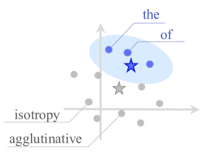
Figure 1: Low-frequent words { &} and high-frequent words { &} are unevenly distributed in the embedding space [39, 24, 44, 10]. Consequently, the “apparent” mean calculated by unweighted averaging ★ often differs from the actual centroid ★.

Let us describe the above idea formally. The data matrix $\boldsymbol{X}\in\mathbb{R}^{n\times d}$ or the set of data vectors $\{\boldsymbol{x}_{i}\}_{i=1}^{n}\subseteq\mathbb{R}^{d}$ represents a collection of instances, observations, or tokens; then the empirical distribution is $\mu_{\boldsymbol{X}}=\sum_{i=1}^{n}\leavevmode\hbox to7.2pt{\vbox to14.19pt{\text{[drawing]}}}\delta(\boldsymbol{x}_{i})$, where $\delta$ is the Dirac delta function. Here, the unweighted mean can be seen as the expectation $\widehat{\operatorname*{\mathbb{E}}}_{\boldsymbol{x}\sim\mu_{\boldsymbol{X}}}[\boldsymbol{x}]=\sum_{i=1}^{n}\leavevmode\hbox to7.2pt{\vbox to14.19pt{\text{[drawing]}}}\boldsymbol{x}_{i}$ with the empirical distribution. On the other hand, the word embedding matrix $\boldsymbol{W}\in\mathbb{R}^{n\times d}$ or the set of word vectors $\{\boldsymbol{w}_{i}\}_{i=1}^{n}\subseteq\mathbb{R}^{d}$ represents a collection of types. When describing the empirical distribution, the hidden frequency $p$ of tokens is necessary. Given $p$, the empirical distribution is $\mu_{\boldsymbol{W}}=\leavevmode\hbox to25.17pt{\vbox to16.67pt{\text{[drawing]}}}\delta(\boldsymbol{w}_{i})$. From this perspective, the centroid of the word vectors should be written as the expectation $\widehat{\operatorname*{\mathbb{E}}}_{\boldsymbol{w}\sim\mu_{\boldsymbol{W}}}[\boldsymbol{w}]=\sum_{i}\leavevmode\hbox to25.17pt{\vbox to16.67pt{\text{[drawing]}}}\boldsymbol{w}_{i}$ over $p$.

The distinction is not just “theoretical.” First, refer to Fig. 1. Word vectors are known to cluster by frequency [39, 24, 44, 10]. In this situation, the centroid ★ weighted by the word frequencies is located near the narrow region where high-frequent words are concentrated (a region with a light blue background), and thus differs from the unweighted mean ★. Second, see Table 1, which shows 50 words sampled from each of types and tokens. Uniform sampling from types, corresponding to an unweighted mean, tends to select mostly rare words from the heavy tail. Sampling from tokens clearly captures a more natural representation of language as it typically appears in text.

Table 1: The difference between type-based sampling and token-based sampling.

Words sampled from

Words sampled from

‘scintillation’, ‘fanon’, ‘rubato’, ‘upstanding’, ‘collard’, ‘creeks’, ‘skookum’, ‘unbelievers’, ‘monocyte’, ‘nishikawa’, ‘crusher’, ‘gerwen’, ‘abrah’, ‘silverchair’, ‘hangman’, ‘unitary’, ‘klausen’, ‘arousal’, ‘heat’, ‘bridgnorth’, ‘mildred’, ‘porton’, ‘aquasox’, ‘wylie’, ‘hipaa’, ‘krimuk’, ‘hexahedron’, ‘kuei’, ‘barbera’, ‘dalvi’, ‘gilding’, ‘visakhapatnam’, ‘tatsuo’, ‘tarascon’, ‘bajram’, ‘scholes’, ‘hadad’, ‘incidental’, ‘theodosius’, ‘reichskommissariat’, ‘boeheim’, ‘amsl’, ‘buencamino’, ‘thrasyvoulos’, ‘insulated’, ‘discourtesy’, ‘nisra’, ‘ycko’, ‘luen’, ‘dooku’

‘nine’, ‘ranked’, ‘zero’, ‘the’, ‘garcia’, ‘rank’, ‘station’, ‘the’, ‘for’, ‘four’, ‘williams’, ‘drunken’, ‘a’, ‘one’, ‘eight’, ‘of’, ‘were’, ‘zero’, ‘debate’, ‘orchestra’, ‘of’, ‘wrist’, ‘points’, ‘fractured’, ‘the’, ‘to’, ‘redirect’, ‘adnan’, ‘white’, ‘car’, ‘fond’, ‘concluded’, ‘under’, ‘two’, ‘by’, ‘five’, ‘his’, ‘infection’, ‘the’, ‘the’, ‘pop’, ‘in’, ‘one’, ‘in’, ‘one’, ‘one’, ‘fram’, ‘handled’, ‘battle’, ‘mutual’

3 Embedding symmetry

3.1 Definition of embedding symmetry

In mathematical science fields, such as high-dimensional probability theory [55] and the volume of convex bodies [27], there are numerous intriguing definitions of spatial symmetry. Among them, we begin with the definition of the symmetry of random vectors with their frequencies [48, 55]. This is suited for dealing with word vectors because they entail word frequencies, unlike usual data instances.

Definition 1 (A random vector $\boldsymbol{v}\sim p$ on $\mathbb{R}^{d}$ has zero mean; the 1st moment of a symmetric random vector).

$\displaystyle\overline{\boldsymbol{v}}\coloneq\mathbb{E}_{\boldsymbol{v}\sim p}[\boldsymbol{v}]=\boldsymbol{0}$ (1)

Definition 2 (A random vector $\boldsymbol{v}\sim p$ on $\mathbb{R}^{d}$ is in isotropic position around its barycenter; the 2nd moment of a symmetric random vector).

$\displaystyle\!\!\!\mathrm{Cov}[\boldsymbol{v}]\!\coloneq\mathbb{E}_{\boldsymbol{v}\sim p}[(\boldsymbol{v}\!-\!\mathbb{E}_{\boldsymbol{v}\sim p}[\boldsymbol{v}])(\boldsymbol{v}\!-\!\mathbb{E}_{\boldsymbol{v}\sim p}[\boldsymbol{v}])^{\!\top\!}]\!\propto\!\boldsymbol{I}_{d}\!\!$ (2)

From these definitions, we will develop methods to adjust given word vectors to be symmetric in § 3.2, and to evaluate the symmetry of given word vectors in § 3.3.

In machine learning and NLP, the spatial symmetry of embedding spaces is a hot topic, and numerous theories and algorithms have been proposed [41, 21, 38, 56]. However, the approach in many researches implicitly treats all vectors equally, ignoring word frequency information. In the following sections, we will detail both the empirical and theoretical issues that a uniform approach can cause, especially when applied to NLP tasks. Furthermore, when embeddings correspond to tokens rather than types—such as in the internal representations of masked or causal language models—a uniform approach tends to be effective. This point will be discussed in § 5.1.

3.2 Enhancement of embedding symmetry

Algorithm 1 Zipfian whitening; a post-processing algorithm on word embeddings. The part highlighted in blue shows the difference from the typical centering and whitening.

1:Word embeddings $\{\boldsymbol{w}_{i}\in\mathbb{R}^{d}\mid w_{i}\in\mathcal{V}\}$, word frequency $\leavevmode\hbox to8.03pt{\vbox to12.92pt{\text{[drawing]}}}\colon\mathcal{V}\to[0,1]$.

2:Processed word embeddings. $\{\overline{\boldsymbol{w}}_{i}\in\mathbb{R}^{d}\}_{i}$ are centered, $\{\widetilde{\boldsymbol{w}}_{i}\in\mathbb{R}^{d}\}_{i}$ are further whitened.​​

3:Zipfian centering (1st moment):

4:$\mathmakebox[1em]{\widehat{\boldsymbol{\mu}}}\leftarrow\sum_{w_{i}\in\mathcal{V}}\leavevmode\hbox to25.17pt{\vbox to16.67pt{\text{[drawing]}}}\boldsymbol{w}_{i}\in\mathbb{R}^{d}$

5:for all $w_{i}\in\mathcal{V}$ do

6:     $\mathmakebox[1em]{\overline{\boldsymbol{w}}_{i}}\leftarrow\boldsymbol{w}_{i}-\widehat{\boldsymbol{\mu}}\in\mathbb{R}^{d}$

7:end for

8:Zipfian decorrelation and standardization (2nd moment):

9:$\mathmakebox[1em]{\boldsymbol{W}_{p}}\leftarrow\left[\leavevmode\hbox to26.04pt{\vbox to16.67pt{\text{[drawing]}}}\,\overline{\boldsymbol{w}}_{1}^{\top},\dots,\leavevmode\hbox to31.88pt{\vbox to19.17pt{\text{[drawing]}}}\,\overline{\boldsymbol{w}}_{\left\lvert\mathcal{V}\right\rvert}^{\top}\right]^{\top}\in\mathbb{R}^{{\left\lvert\mathcal{V}\right\rvert}\times d}$

10:$\mathmakebox[1em]{\boldsymbol{U}\boldsymbol{\Sigma}\boldsymbol{V}^{\top}}\leftarrow\mathrm{SVD}(\boldsymbol{W_{p}})$

11: $\triangleright$$\boldsymbol{\Sigma}=\mathrm{diag}(\sigma_{1},\dots,\sigma_{d})\in\mathbb{R}^{d\times d}$ consists of the singular values of $\boldsymbol{W}_{p}$.

12:for all $w_{i}\in\mathcal{V}$ do

13:     $\mathmakebox[1em]{\widetilde{\boldsymbol{w}}_{i}}\leftarrow\overline{\boldsymbol{w}_{i}}\boldsymbol{V}\boldsymbol{\Sigma}^{-1}$

14:      $\triangleright$$\boldsymbol{\Sigma}^{-1}:=\mathrm{diag}(1/\sigma_{1},\dots,1/\sigma_{d})\in\mathbb{R}^{d\times d}$.

15:end for

This section proposes Zipfian whitening, which symmetrizes a given set of word vectors with word frequency. At a glance, the most natural method to achieve Def. 1 and Def. 2 would be PCA whitening, also known as sphering. Notably, each step of whitening—centering, decorrelation, and standardization—implicitly involves calculating expected values. Our approach is simple: each time we calculate an expected value, we should weight it by the empirical word frequency. The specific algorithm is as shown in Algorithm 1. The only difference from general whitening is that it uses word frequency in . Please refer to Appendix A for a formal explanation showing that the word vectors obtained by the proposed algorithm actually satisfy Def. 1 and Def. 2.

Empirical evaluation:

We confirm the effectiveness of Zipfian whitening (Algorithm 1) by measuring performance on standard sentence-level downstream tasks using post-processed word vectors. We employed the most standard word embeddings—GloVe [43], word2vec [37], and fastText [11]—and utilized the widely adopted evaluation tasks, including STS-B [15] and related benchmarks. Detailed experimental settings can be found in Appendix B. Table 2 shows the results on the STS-B task. Remarkably, the proposed Zipfian whitening shows significant advantages not only over standard (uniform) centering and whitening but also over the strong baseline method [7] specifically designed to create powerful sentence vectors. Consistent results were obtained with various benchmark datasets, multiple empirical word probabilities, and a language other than English (Appendix C). In § 4.2, one reason for this remarkable performance is clarified from the perspective of information geometry.

Table 2: The empirical performance of Zipfian whitening, which exploits the empirical frequency of words during expectation calculations. Each cell shows the STS-B [15] score $\times 100$. By carefully performing the simple operation of whitening, it consistently outperforms powerful baseline methods.

GloVe	46.17
	Uniform	Zipfian
+ Centering	45.17	52.25
+ Whitening	52.21	66.92
+ ABTT [39]	54.28
+ SIF + CCR [7]	58.70

Word2Vec	56.98
	Uniform	Zipfian
+ Centering	55.85	58.84
+ Whitening	56.03	66.50
+ ABTT [39]	56.98
+ SIF + CCR [7]	63.04

3.3 Evaluation of embedding symmetry

The community is greatly interested not only in making word vector spaces symmetric but also in evaluating how symmetric or asymmetric a space is [21, 49]. Here, we return to Def. 1 and Def. 2 and describe metrics for evaluating the symmetry of word embedding spaces with word frequency.

Degree of centrality—the 1st moment of symmetry:

Recall that, if the barycenter $\operatorname*{\mathbb{E}}[\boldsymbol{v}]$ is close to $\boldsymbol{0}$, then the random vector $\boldsymbol{v}$ can be considered symmetric in terms of the first moment (Def. 1). Thue, examining the value of $\left\lVert\operatorname*{\mathbb{E}}[\boldsymbol{v}]\right\rVert\coloneq\operatorname*{\mathbb{E}}[\boldsymbol{v}]-\boldsymbol{0}$ appears to be a reasonable way to measure the symmetry of the first moment. However, random vectors $\boldsymbol{v}$ and $\alpha\boldsymbol{v}$ ($\alpha\in\mathbb{R}_{>0}$) should be considered equivalent in terms of spatial symmetry. Thus, we define the scale-invariant metric (Def. 3), obtained by dividing $\left\lVert\operatorname*{\mathbb{E}}[\boldsymbol{v}]\right\rVert$ by the average length $\operatorname*{\mathbb{E}}[\left\lVert\boldsymbol{v}\right\rVert]$.

Definition 3 (Degree of centrality for the random vector $\boldsymbol{v}\sim p$; the 1st moment of symmetry).

$\displaystyle\mathrm{Sym}_{1}(\boldsymbol{v})\coloneqq 1-\left\lVert\operatorname*{\mathbb{E}}_{\boldsymbol{v}\sim p}[\boldsymbol{v}]\right\rVert/\operatorname*{\mathbb{E}}_{\boldsymbol{v}\sim p}[\left\lVert\boldsymbol{v}\right\rVert]$ (3) By definition, $\mathrm{Sym}_{1}(\boldsymbol{v})$ takes values in $[0,1]$, and $\mathrm{Sym}_{1}(\boldsymbol{v})=1$ if and only if $\boldsymbol{v}$ is zero mean.

Degree of isotropy—the 2nd moment of symmetry:

If the covariance matrix $\mathbb{E}[(\boldsymbol{v}-\mathbb{E}[\boldsymbol{v}])(\boldsymbol{v}-\mathbb{E}[\boldsymbol{v}])^{\top}]$ is a constant multiple of the identity matrix $\boldsymbol{I}_{d}$, i.e., if the random vector $\boldsymbol{v}$ has an equal spread in all directions, $\boldsymbol{v}$ is symmetric in terms of the second moment (Def. 2). Following convention, this degree can be confirmed by examining the flatness of the eigenspectrum.

Definition 4 (Degree of isotropy around the barycenter for the random vector $\boldsymbol{v}\sim p$; the 2nd moment of symmetry).

$\displaystyle\mathrm{Sym}_{2}(\boldsymbol{v})\coloneqq\frac{1}{\log d}H\left(\frac{\lambda_{1}}{\sum_{j}\lambda_{j}},\dots,\frac{\lambda_{d}}{\sum_{j}\lambda_{j}}\right)$ (4) $\displaystyle\{\lambda_{1},\dots,\lambda_{d}\}\;\text{are the eigenvalues of the covariance matrix}\;\operatorname*{\mathbb{E}}_{\boldsymbol{v}\sim p}[(\boldsymbol{v}-\operatorname*{\mathbb{E}}_{\boldsymbol{v}\sim p}[\boldsymbol{v}])(\boldsymbol{v}-\operatorname*{\mathbb{E}}_{\boldsymbol{v}\sim p}[\boldsymbol{v}])^{\top}]\text{.}$ $\displaystyle\textstyle H(p_{1},\dots,p_{d})\coloneqq-\sum_{i}p_{i}\log p_{i}\;\text{is the Shannon entropy.}$

Proposition 1.

$\mathrm{Sym}_{2}(\boldsymbol{v})$ takes values in $[0,1]$, and $\mathrm{Sym}_{2}(\boldsymbol{v})=1$ if and only if $\boldsymbol{v}$ is isotropic around its barycenter (Def. 2). Proof. Please refer to Appendix D.

Note that the approach of measuring the entropy of the spectrum to evaluate the flatness of a signal can be found in many fields. For example, similar definitions are seen in probability processes [14] and signal processing [17, 47]. We also follow this standard and powerful line.

Algorithm:

To compute the evaluation metrics of symmetry (Def. 3, Def. 4) for given word vectors, again, one should just use the empirical word frequency when calculating the expectations. A pseudocode for measuring symmetry is provided in Appendix E.

Empirical evaluation:

To what extent does our symmetry score (an intrinsic evaluation of embedding spaces) correlate with downstream task performance (an extrinsic evaluation of those)? As baselines, we use versions of our symmetry score that do not account for word frequency, calculated in a uniform manner. We also compare with popular symmetry scores in NLP, the average of cosine similarity (Ave. Cos.) [21] and the recently proposed IsoScore [49]. Note that all these baselines implicitly assume uniform word frequency. Additional experimental settings can be found in Appendix B. Fig. 2 shows the results. The right side of Fig. 2 demonstrates the superiority of the Zipfian approach. Moving from the bottom-left to the top-right of the figure—i.e. as both the 1st ($x$-axis) and 2nd moments ($y$-axis) of the symmetry score increase—it is clearly visible that the downstream task performance increases (the color becomes more red). In contrast, in the left-hand plot, which assumes uniform word frequency, there is no observed relationship between the symmetry score ($x$ and $y$-axis) and the downstream task performance (color). Table 3 lists the correlation coefficients between the symmetry scores and downstream task performance in more detail. It can be seen that the symmetry scores can “predict” downstream task performance with remarkably high correlation. On the other hand, the “prediction” performance of other metrics, including Ave. Cos. and IsoScore that implicitly assume , is unsatisfactory. Surprisingly, when the most popular Ave. Cos. metric shows almost no correlation ($0.04$) with downstream task performance (STS-B), Zipfian symmetry metric has a strong positive correlation ($0.83$) with it.

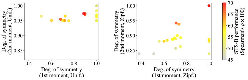
Figure 2: The relationship between the 1st-order symmetry (Def. 3, $x$-axis), the 2nd-order symmetry (Def. 4, $y$-axis), and task performance (color). Each point represents either pre-trained or post-processed word embeddings (GloVe, word2Vec, and fastText). The Zipfian measure well captures the downstream task performance (right), while the uniform isotropic measure cannot (left).

Table 3: Spearman’s $\rho\times 100$ (each cell) between the symmetry scores (each column) and downstream STS-B performance (each row), on pre-trained and post-processed embeddings (GloVe, word2Vec, and fastText). The scores based on the Zipfian prior show a significantly higher correlation with task performance compared to those based on the uniform prior including Ave. Cos. and IsoScore.

	Ave. Cos.	IsoScore	Uniform		Zipfian
	[21]	[49]	1st moment	2nd moment	1st moment	2nd moment
STS-B	$-6.95$	$0.07$	$-21.91$	$-21.21$	$62.13$	89.55
SICK-R	$20.09$	$18.41$	$13.26$	$-8.71$	$60.04$	64.60

4 Why is Zipfian whitening better than uniform whitening?

A natural question is why the Zipfian approach empirically dramatically outperforms the uniform approach. We provide a theoretical explanation using Table 4. In a nutshell, a significant difference arises depending on whether the base measure of an exponential family is uniform or Zipfian.

Table 4: Through the differences in the underlying generative models, the empirical superiority of Zipfian whitening over uniform whitening can be understood.

Generative models behind the (whitened) embeddings
$\begin{aligned} &p(w\mid c)=\frac{\pi(w)\exp(\langle\boldsymbol{w},\boldsymbol{c}\rangle)}{Z(c)}\text{,}&&Z(c)=\sum_{w}\pi(w)\exp(\langle\boldsymbol{w},\boldsymbol{c}\rangle)\text{;}&&p(w,c)=p(w\mid c)\pi(c)\end{aligned}$ (5)
with Uniform prior $\displaystyle p_{\mathchoice{\leavevmode\hbox to5.76pt{\vbox to5.76pt{\text{[drawing]}}}}{\leavevmode\hbox to5.76pt{\vbox to5.76pt{\text{[drawing]}}}}{\leavevmode\hbox to4.55pt{\vbox to4.55pt{\text{[drawing]}}}}{\leavevmode\hbox to3.75pt{\vbox to3.75pt{\text{[drawing]}}}}}(w\mid c)=\frac{\leavevmode\hbox to7pt{\vbox to10.49pt{\text{[drawing]}}}\exp(\langle\boldsymbol{w},\boldsymbol{c}\rangle)}{Z_{\mathchoice{\leavevmode\hbox to5.76pt{\vbox to5.76pt{\text{[drawing]}}}}{\leavevmode\hbox to5.76pt{\vbox to5.76pt{\text{[drawing]}}}}{\leavevmode\hbox to4.55pt{\vbox to4.55pt{\text{[drawing]}}}}{\leavevmode\hbox to3.75pt{\vbox to3.75pt{\text{[drawing]}}}}}(c)}\text{,}\;\pi(c)\propto\leavevmode\hbox to7pt{\vbox to10.49pt{\text{[drawing]}}}$ (6)	with Zipfian prior $\displaystyle p_{\mathchoice{\leavevmode\hbox to5.49pt{\vbox to5.49pt{\text{[drawing]}}}}{\leavevmode\hbox to5.49pt{\vbox to5.49pt{\text{[drawing]}}}}{\leavevmode\hbox to4.37pt{\vbox to4.37pt{\text{[drawing]}}}}{\leavevmode\hbox to3.62pt{\vbox to3.62pt{\text{[drawing]}}}}}(w\mid c)=\frac{\leavevmode\hbox to19.19pt{\vbox to13.33pt{\text{[drawing]}}}\exp(\langle\boldsymbol{w},\boldsymbol{c}\rangle)}{Z_{\mathchoice{\leavevmode\hbox to5.49pt{\vbox to5.49pt{\text{[drawing]}}}}{\leavevmode\hbox to5.49pt{\vbox to5.49pt{\text{[drawing]}}}}{\leavevmode\hbox to4.37pt{\vbox to4.37pt{\text{[drawing]}}}}{\leavevmode\hbox to3.62pt{\vbox to3.62pt{\text{[drawing]}}}}}(c)}\text{,}\;\pi(c)=\leavevmode\hbox to16.71pt{\vbox to13.33pt{\text{[drawing]}}}$ (7)
Partition functions become constant under certain conditions
Assume $\left\lVert\boldsymbol{c}\right\rVert\equiv 1$, $\left\lvert\mathcal{V}\right\rvert\to\infty$, then $\displaystyle Z_{\mathchoice{\leavevmode\hbox to5.76pt{\vbox to5.76pt{\text{[drawing]}}}}{\leavevmode\hbox to5.76pt{\vbox to5.76pt{\text{[drawing]}}}}{\leavevmode\hbox to4.55pt{\vbox to4.55pt{\text{[drawing]}}}}{\leavevmode\hbox to3.75pt{\vbox to3.75pt{\text{[drawing]}}}}}(c)\coloneqq\sum_{w}\exp(\langle\boldsymbol{w},\boldsymbol{c}\rangle)=\text{const.}$ (8) [6]	At the optimal solution of the corresponding loss, $\displaystyle Z_{\mathchoice{\leavevmode\hbox to5.49pt{\vbox to5.49pt{\text{[drawing]}}}}{\leavevmode\hbox to5.49pt{\vbox to5.49pt{\text{[drawing]}}}}{\leavevmode\hbox to4.37pt{\vbox to4.37pt{\text{[drawing]}}}}{\leavevmode\hbox to3.62pt{\vbox to3.62pt{\text{[drawing]}}}}}(c)\coloneqq\sum_{w}\leavevmode\hbox to19.19pt{\vbox to13.33pt{\text{[drawing]}}}\exp(\langle\boldsymbol{w},\boldsymbol{c}\rangle)=\text{const.}$ (9) [32]
Whitening coarsely achieves a constant partition function
$Z_{\mathchoice{\leavevmode\hbox to5.76pt{\vbox to5.76pt{\text{[drawing]}}}}{\leavevmode\hbox to5.76pt{\vbox to5.76pt{\text{[drawing]}}}}{\leavevmode\hbox to4.55pt{\vbox to4.55pt{\text{[drawing]}}}}{\leavevmode\hbox to3.75pt{\vbox to3.75pt{\text{[drawing]}}}}}(c)$ $\displaystyle\begin{aligned} &\!\!=\!\left\lvert\mathcal{V}\right\rvert\!&&+\!\biggl{(}\!\wavyunderline{\sum_{w}\boldsymbol{w}}\!\!\biggr{)}^{\!\!\!\top\!\!}\boldsymbol{c}&&+\frac{1}{2}\boldsymbol{c}^{\!\top\!}\!\biggl{(}\!\wavyunderline{\sum_{w}\boldsymbol{w}\boldsymbol{w}^{\!\top\!}}\!\biggr{)}\boldsymbol{c}+\dots\\ {}&\!\!\!\leadsto\!\left\lvert\mathcal{V}\right\rvert\!&&+\wavyunderline{\boldsymbol{0}}^{\top}\boldsymbol{c}&&+\frac{1}{2}\boldsymbol{c}^{\!\top\!}\!\wavyunderline{\boldsymbol{I}}\boldsymbol{c}\dots\!\approx\text{const.}\,(10)\text{\cite[cite]{[\@@bibref{Number}{mu2018allbutthetop}{}{}]}}\end{aligned}$	$Z_{\mathchoice{\leavevmode\hbox to5.49pt{\vbox to5.49pt{\text{[drawing]}}}}{\leavevmode\hbox to5.49pt{\vbox to5.49pt{\text{[drawing]}}}}{\leavevmode\hbox to4.37pt{\vbox to4.37pt{\text{[drawing]}}}}{\leavevmode\hbox to3.62pt{\vbox to3.62pt{\text{[drawing]}}}}}(c)$ $\displaystyle\begin{aligned} &\!\!=\!\left\lvert\mathcal{V}\right\rvert\!&&+\!\biggl{(}\!\wavyunderline{\sum_{w}\leavevmode\hbox to19.19pt{\vbox to13.33pt{\text{[drawing]}}}\boldsymbol{w}}\!\!\biggr{)}^{\!\!\!\top\!\!}\boldsymbol{c}&&+\frac{1}{2}\boldsymbol{c}^{\!\top\!}\!\biggl{(}\!\wavyunderline{\sum_{w}\leavevmode\hbox to19.19pt{\vbox to13.33pt{\text{[drawing]}}}\boldsymbol{w}\boldsymbol{w}^{\!\top\!}}\!\biggr{)}\boldsymbol{c}+\dots\\ {}&\!\!\!\leadsto\!\left\lvert\mathcal{V}\right\rvert\!&&+\wavyunderline{\boldsymbol{0}}^{\top}\boldsymbol{c}&&+\frac{1}{2}\boldsymbol{c}^{\!\top\!}\!\wavyunderline{\boldsymbol{I}}\boldsymbol{c}\dots\!\approx\text{const.}\,(11)\text{[ours]}\end{aligned}$
Vector norm under generative models
$\left\lVert\boldsymbol{w}\right\rVert_{2}^{2}\approx 2d\log p(w)-2Z$ (12) [6] long vector $\leftrightarrow$ frequent (uninformative) word	$\left\lVert\boldsymbol{w}\right\rVert_{\boldsymbol{G}(w)}^{2}\approx 2\mathrm{KL}(p(\cdot)||p(\cdot\mid w))$ (13) [42] [Thm. 1] long vector $\leftrightarrow$ informative word
Loss and error corresponding to generative models $p(w\mid c)$
softmax cross-entropy loss $\displaystyle\operatorname*{\mathbb{E}}_{(w,c)}-\log\frac{\exp(\langle\boldsymbol{w},\boldsymbol{c}\rangle)}{Z_{\mathchoice{\leavevmode\hbox to5.76pt{\vbox to5.76pt{\text{[drawing]}}}}{\leavevmode\hbox to5.76pt{\vbox to5.76pt{\text{[drawing]}}}}{\leavevmode\hbox to4.55pt{\vbox to4.55pt{\text{[drawing]}}}}{\leavevmode\hbox to3.75pt{\vbox to3.75pt{\text{[drawing]}}}}}(c)}$ (14)	logit-adjusted softmax cross-entropy loss $\displaystyle\operatorname*{\mathbb{E}}_{(w,c)}-\log\frac{\leavevmode\hbox to19.19pt{\vbox to13.33pt{\text{[drawing]}}}\exp(\langle\boldsymbol{w},\boldsymbol{c}\rangle)}{Z_{\mathchoice{\leavevmode\hbox to5.49pt{\vbox to5.49pt{\text{[drawing]}}}}{\leavevmode\hbox to5.49pt{\vbox to5.49pt{\text{[drawing]}}}}{\leavevmode\hbox to4.37pt{\vbox to4.37pt{\text{[drawing]}}}}{\leavevmode\hbox to3.62pt{\vbox to3.62pt{\text{[drawing]}}}}}(c)}$ (15) [36]
misclassification error $\displaystyle\mathbb{P}_{(w,c)}[w\not\in\operatorname*{arg\,max}_{w^{\prime}}\langle\boldsymbol{w}^{\prime},\boldsymbol{c}\rangle]$ (16)	balanced error $\textstyle\frac{1}{\left\lvert\mathcal{V}\right\rvert}\displaystyle\sum_{w\in\mathcal{V}}\mathbb{P}_{c\mid w}[w\not\in\operatorname*{arg\,max}_{w^{\prime}}\langle\boldsymbol{w}^{\prime},\boldsymbol{c}\rangle]$ (17) [36]

4.1 Characterization through generative model, partition function, and whitening

Exponential families:

Hereafter, we interpret two salient generative models from the viewpoint of exponential families: one given by Arora et al. [6] and the other generalizing the Levy–Goldberg formula [32, Eq. (7)]. Details of these models will be provided shortly. An exponential family is a class of probability distributions of a random variable $\boldsymbol{x}$ parametrized by a parameter $\boldsymbol{\theta}$, written in the following (canonical) form:

$$\!\!p(\boldsymbol{x}\mid\boldsymbol{\theta})=\pi(\boldsymbol{x})\exp\left(\langle\boldsymbol{x},\boldsymbol{\theta}\rangle-\psi(\boldsymbol{\theta})\right),\quad\psi(\boldsymbol{\theta})\coloneqq\log Z(\boldsymbol{\theta})=\log\left(\sum_{\boldsymbol{x}}\pi(\boldsymbol{x})\exp(\langle\boldsymbol{x},\boldsymbol{\theta}\rangle)\!\right),\!$$ (18)

where $\boldsymbol{x}$ is a sufficient statistic, $\boldsymbol{\theta}$ is called a natural parameter, $\pi$ is the base measure (or “prior”), and $\psi$ is the log-partition function. Once we specify the base measure $\pi$ and the canonical pair $(\boldsymbol{x},\boldsymbol{\theta})$, the log-partition function is determined. That being said, the base measure $\pi$ is the design choice of an exponential family left for us. In the following, we specifically examine an exponential family of distributions in the form $p(w\mid c)$, where word $w$ is predicted given context $c$. Specifically, the context represents a co-occurring word (in static word embeddings), a cloze sentence (in masked language models), or a sentence prefix (in causal language models). In all of these cases, we predict a word with the logit $\langle\boldsymbol{w},\boldsymbol{c}\rangle$, making the exponential family a natural probabilistic model. Here, the vector $\boldsymbol{c}$ represents the vector expression of the context $c$, known as the “context vector.” Note that, even for the same word $t$, the predicted word vector $\boldsymbol{w}(t)$ and the predicting context vector $\boldsymbol{c}(t)$ are distinct.

Uniform prior:

Arora et al. firstly considered a log-linear generative model of word embeddings given a context (4) and demonstrated that when the generative model is adopted with normalized context vectors and a huge vocabulary, the partition function asymptotically becomes constant (4) [6, Lemma 2.1]. Here, we can regard that this model belongs to the exponential family with the uniform base measure $\pi(w)=\pi(c)=\leavevmode\hbox to28.28pt{\vbox to16.67pt{\text{[drawing]}}}$ .

Zipfian prior:

An exponential family adopted with the Zipfian measure can be written as (4). This generative model can be naturally derived from the skip-gram model with negative sampling (SGNS) [37]. By assuming that the linear model $c\mapsto\langle\boldsymbol{w},\boldsymbol{c}\rangle$ is sufficiently capable of discriminating cooccurring words and negative samples (as in the realizable case), we can see that the generative model of the word embeddings must comply with the following formula:

$$\log\frac{p(w,c)}{p(w)p(c)}-\log k=\langle\boldsymbol{w},\boldsymbol{c}\rangle\text{,}$$ (19)

where $k$ is the number of negative samples. This optimality formula owes to Levy and Goldberg [32], and we call (19) the Levy–Goldberg formula. A more concise derivation is later given by Oyama et al. [42]. We can regard the Levy–Goldberg formula as an exponential family with the Zipfian base measure, $\pi(w)=\leavevmode\hbox to23.24pt{\vbox to16.67pt{\text{[drawing]}}}$ and $\pi(c)=\leavevmode\hbox to20.14pt{\vbox to16.67pt{\text{[drawing]}}}$, and the constant log-partition function $Z_{\mathchoice{\leavevmode\hbox to6.76pt{\vbox to6.76pt{\text{[drawing]}}}}{\leavevmode\hbox to6.76pt{\vbox to6.76pt{\text{[drawing]}}}}{\leavevmode\hbox to5.36pt{\vbox to5.36pt{\text{[drawing]}}}}{\leavevmode\hbox to4.42pt{\vbox to4.42pt{\text{[drawing]}}}}}(c)\equiv k^{-1}$. The generative model (4) is a relaxation of the Levy–Goldberg formula since we do not impose the realizability assumption necessary for the derivation of (19).

What does whitening do?

Mu and Viswanath [39] proposed a method to approximately make the partition function of the uniform prior model constant by centering the word vectors and removing the top principal components (4). Our Zipfian whitening corresponds to Mu and Viswanath’s post-processing method, in the sense that ours and theirs make the partition function constant up to the second moment (4) and (4), respectively. In summary, Zipfian whitening (4) transforms a probabilistic model into an exponential family adopted with the Zipfian base measure (4), making it closer to the Levy–Goldberg formula (19).

4.2 Emphasis on rare words by Zipfian prior

Let us explore further why the Zipfian prior results in good performance in downstream tasks (§ 3.2). In summary, the Zipfian prior approach emphasizes low-frequency words, while the uniform prior approach emphasizes high-frequency words, both from perspectives of vector norms and errors/losses. So far in this paper, we have repeatedly discussed weighting each word according to frequency, so it may seem contradictory that Zipfian approach emphasizes low-frequency words as a result. To illustrate, let us reconsider centering. In centering, the mean vector is subtracted from each vector. Weighting each word vector by frequency when constructing the mean vector means that signals corresponding to high-frequency words are removed more substantially from each vector. The emphasis on low-frequency words has been repeatedly supported throughout the history of NLP and information retrieval, such as Luhn’s hypothesis [34], inverse document frequency (IDF) [53], and smooth inverse frequency (SIF) [7]. For instance, it is reasonable to emphasize the word ‘isotropy’ when creating a sentence embedding containing both words ‘the’ and ‘isotropy’.

From the perspective of vector norm

Under the Zipfian prior model, words with larger information content have longer (emphasized) vector representations. Conversely, under the uniform prior model, words with smaller information content have longer (emphasized) vector representations.

As a representative example of uniform prior models, the norms of word vectors learned by random walk language models are theoretically and empirically proportional to word frequency (4) (see Eq. (2.4) and Fig. 2 in Arora et al. [6]). That is, in such embedding space, words with less information (e.g., ‘the’) are emphasized. This tendency is consistently observed in dynamic language models and causal language models that adopt the softmax cross-entropy loss, another typical example of the uniform prior family [28]. By contrast, when training word embeddings with skip-gram negative sampling [37], the word embeddings follow the Zipfian prior family, and their norms become larger with greater information, which we show subsequently [50, 60, 42]. Based on the formulation of the exponential family and following Eq. (12) of Oyama et al. [42], we formally describe the norm properties of the word vectors obtained from the Zipfian prior model.

Theorem 1 (The norm of a word vector learned with empirical Zipfian prior models reflect the information amount of the word; a refined version of [42] Eq. (12)).

Assume that word embeddings $\{\boldsymbol{w}_{i}\}_{i}$ follow the Zipfian prior model (4), For the same word $t$, the vector $\boldsymbol{w}$ on the predicted side and the vector $\boldsymbol{c}$ on the predicting side are shared: $\boldsymbol{w}(t)\equiv\boldsymbol{c}(t)$ (weight tying), and $\sum_{t\in\mathcal{V}}p(t)\boldsymbol{w}(t)=\boldsymbol{0}$ (centered w.r.t. Zipfian prior), then each word vector $\boldsymbol{w}(t)$ satisfy

$$\left\lVert\boldsymbol{w}(t)\right\rVert_{\boldsymbol{G}(t)}^{2}\approx 2\mathrm{KL}(p(\cdot)\|p(\cdot\mid t))\text{,}\quad\boldsymbol{G}(t)\coloneqq\sum_{t^{\prime}\in\mathcal{V}}p(t^{\prime}\mid t)\boldsymbol{c}(t^{\prime})\boldsymbol{c}(t^{\prime})^{\top}\text{,}$$ (20)

where $\left\lVert\boldsymbol{w}\right\rVert_{\boldsymbol{A}}$ with a positive definite matrix $\boldsymbol{A}$ denote a norm based on a quadratic form $\sqrt{\boldsymbol{w}^{\top}\boldsymbol{A}\boldsymbol{w}}$.
Proof. Refer to Appendix F.

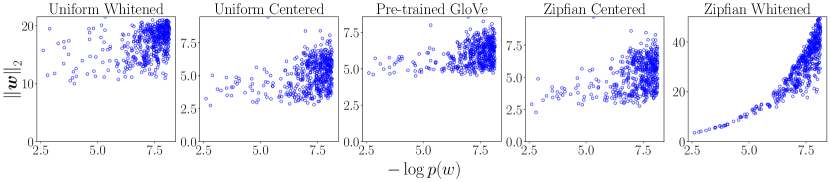
Figure 3: Relationships between the information content $-\log{p(w)}$ and the vector norms $\lVert\boldsymbol{w}\rVert_{2}$ for top 500 frequent words $w$. The figure in the center represents the pre-trained GloVe model. By using Zipfian whitening, the information content gets encoded in the norm (center to right). Conversely, with uniform whitening, this phenomenon does not occur (center to left).

In Fig. 3, we experimentally confirmed that the norms of informative words become larger with Zipfian whitening (shown from center to the right in Fig. 3), bringing them closer to the ideal Zipfian prior model.

From the perspective of error and loss

The error and loss functions associated with the Zipfian prior model emphasize low-frequency words. In contrast, the error and loss functions of the uniform prior model focus on the average loss across the entire dataset, resulting in a greater emphasis on high-frequency words.

The standard classification loss is the softmax cross-entropy loss (4). By taking its expectation over the dataset $\{(w,c)\}$, embeddings associated with higher-frequency words receive more updates because the softmax is the uniform inverse link, corresponding to the uniform prior model. By contrast, the logit-adjusted loss (4) has been proposed to tackle class imbalance [36]. From our viewpoint, the logit adjustment term $p(w)$ makes the inverse link belong to the Zipfian prior model. The softmax and logit-adjusted losses are Fisher consistent to the misclassification (4) and balanced (4) error rates, respectively. As the latter tends to stress minor classes, the logit-adjusted loss and Zipfian prior model are suitable for emphasizing low-frequency words during the learning process.

Another prominent loss function for representation learning is contrastive loss, with the SGNS loss (word2vec) [37] as a representative example in the context of word representation learning. This loss similarly uses a loss aligned with the Zipfian prior:

$$-\operatorname*{\mathbb{E}}_{(w,c)}\Biggl{[}\log\sigma(\langle\boldsymbol{w},\boldsymbol{c}\rangle)+\sum_{w_{i}^{\prime}\sim\;\leavevmode\hbox to17.17pt{\vbox to11.67pt{\text{[drawing]}}}}^{i=1,\dots,k}\log\sigma(-\langle\boldsymbol{w}_{i}^{\prime},\boldsymbol{c}\rangle)\Biggr{]}\text{,} p(w) p(w)$$ (21)

where $\sigma$ is sigmoid function, and $k$ is the number of negative samples. Since high-frequency words are more likely to be sampled as negative examples, the loss has less impact on high-frequency words in positive examples. Consequently, low-frequency positive words are relatively emphasized in representation learning. The Levy–Goldberg formula in the previous section describes the properties of an ideally trained word2vec model, which are essentially the properties of Zipfian prior models.

5 Unified explanation of the efficacy of existing methods

Distinguishing the distribution that the base measure follows helps us understand why some existing NLP methods are effective.

5.1 Uniform whitening of token embeddings $\approx$ Zipfian whitening of type embeddings

Masked language models like BERT [18] and RoBERTa [33] produce dynamic (contextualized) token embeddings. Adding up such token embeddings of constituent tokens to create sentence embeddings often leads to poor empirical performance [46]. However, symmetrizing significantly improves their performance; such methods including “batch centering,” “WhiteningBERT,” and contrastive learning methods [16, 46, 59, 22, 26, 57]. This improvement can also be explained from the perspective of the Zipfian prior. A dataset or corpus is first fed into the model to obtain token embeddings. Centering/whitening is then applied to this entire set of embeddings. As this token embedding (multi)set has the multiplicity asymptotically proportional to the word frequency, this uniform centering/whitening of token embeddings corresponds to the word-frequency-weighted (Zipfian) centering/whitening of type embeddings. For a more formal description of the above explanations, please refer to Appendix H. Additionally, recent work has found that contrastive additive sentence encoders implicitly weight words by their information content [30]. This finding is consistent with the previous discussion on vector norms (§ 4.2), and can be seen as indirect evidence supporting the idea that these models belong to the Zipfian prior family.

This idea can also be supported by empirical evidence. This idea is also supported by empirical evidence. To establish a baseline for centering and whitening token embeddings under a uniform prior, we scale each embedding by the reciprocal of its type frequency, ensuring uniform treatment across types. Refer to the Appendix H for the detailed computation of this pseudo uniform approach and a formal explanation of how it achieves type uniformity. Table 5 shows the results. Comparing the pseudo-uniform centering/whitening (which assumes a uniform prior over types) with the conventional token-level uniform centering/whitening (which implicitly assumes a Zipfian prior over types) reveals that the latter approach based on a Zipfian prior empirically achieves better performance. Additional experimental settings and results can be found in Appendix B and Appendix I.

Table 5: The empirical performance difference between “uniform”—enforced centering and whitening with a uniform prior for dynamic embeddings, and “Zipfian”—conventional uniform centering and whitening over tokens with an implicit Zipfian prior over types. Each cell shows the STS-B [15] score $\times 100$. This comparison reveals that token-level uniform centering/whitening, corresponding to type-level Zipfian centering/whitening, leads to empirically better performance.

BERT-base	63.75
	“Uniform”	“Zipfian”
+ Centering	64.04	64.82
+ Whitening	60.53	64.91

RoBERTa-base	⁢60.75⁢⁢
	“Uniform”	“Zipfian”
+ Centering	⁢60.34⁢⁢	⁢61.30⁢
+ Whitening	⁢61.31⁢⁢	⁢65.59⁢

5.2 Headless causal language model roughly belongs to Zipfian prior family

The recently proposed headless language model [23] uses only words within the same batch to predict next tokens with a pseudo-softmax function. This method originally aimed to reduce the computational cost of the softmax function in the $\lvert\mathcal{V}\rvert$ direction, but an interesting side effect is the improvement in the performance. This success can also be explained from the perspective of Zipfian priors. If we repeatedly sample small batches, the sampling frequency of each word will increasingly reflect its true frequency as the batch size approaches $1$.

6 Conclusion

Standard methods for adjusting and measuring symmetries in word embedding spaces—such as centering and whitening—implicitly assume uniformly distributed word frequencies, which is unrealistic. We hypothesize that, based on the type-token distinction, using empirical Zipfian word frequencies is essential when calculating the expectation (§ 2). Based on the idea and the definitions of first- and second-order symmetry in random vectors, we derived Zipfian whitening, which enhances the symmetry of the word embedding space. Even though it is nearly identical to standard PCA whitening, Zipfian whitening significantly outperforms existing methods (§ 3.2). Similarly, we derived a metric to evaluate the symmetry of word embedding spaces. Our intrinsic metrics showed a strong correlation with extrinsic task performance, even when popular metrics show almost none (§ 3.3). We then presented a framework explaining the differences in effect between whitening based on uniform and Zipfian approaches, by attributing them to differences in the base measure of the exponential family (§ 4.1). By further exploring this viewpoint through information geometry and loss functions, we showed how the Zipfian approach emphasizes the informativeness of low-frequency words (§ 4.2). Lastly, through our proposed viewpoint, we found that popular NLP methods perform well because their word embeddings end up encoding a Zipfian prior; such models include word2vec [37] (§ 4.2), WhiteningBERT [26] (§ 5.1), and headless language models [23] (§ 5.2).

Limitations

How these assumptions might be violated in practice

In our theoretical analysis concerning norms, and in the discussion on the relationship between whitening and normalization constants, we have proceeded by ignoring the residual terms beyond the second order. Empirically, focusing only on the first and second order has yielded significant results. However, to accurately identify cases where the proposed method might fail, a detailed theoretical and empirical examination of the asymptotic behavior of higher-order moments might be crucial. This remains an important future work.

The condition that the partition function is constant is only a necessary condition from the perspective of both the generative model’s optimal solution and whitening. The true logical relationship between whitening and the generative model has not been clarified. In particular, verifying whether the projection through whitening allows us to transition between the two model families (the uniform family and the Zipfian family) is an intriguing and valuable direction for both theoretical exploration and practical application.

The scope of the empirical claims made

Our experiments primarily focused on static and dynamic word embeddings, as many of their theoretical properties have been understood and they have been central to the rise of isotropization. Admittedly, this paper also advances our understanding of causal language models. However, to make a more significant practical impact in the era of large language models, employing the proposed method as a regularization term for next-token prediction holds great promise for future work.

The experiments utilized typical downstream NLP tasks, particularly popular datasets for sentence-level semantic tasks. By scaling up the task set to include word-level tasks or leveraging a broader range of multilingual data, we can more robustly demonstrate the practical utility of the proposed framework.

The factors that influence the performance of our approach

The proposed method inherently involves numerically unstable calculations, such as multiplying by the inverse of small singular values. Embeddings for low-frequency words are often far from converged even after extensive pre-training, and the eigenvalues of the embedding space are known to decay. Given these situations, the adverse effects of small singular values are plausible. Considering recent advancements in whitening techniques, developing a more numerically stable algorithm is an important direction for future work.

Broader Impacts

Potential impacts to AI alignment

Dohmatob et al. [19] reported that repeated sampling from generative AIs may shift word frequency distributions toward lighter-tailed distributions. This may reduce linguistic diversity and lead to cultural homogenization by diminishing region-specific or culturally unique expressions. Our Zipfian whitening and similar regularization methods could enhance output diversity, enriching the linguistic landscape.

Potential negative societal impacts

The sentence similarity tasks used in our evaluation experiments are now considered core technologies for RAG (retrieval-augmented generation), which is essential when large language models leverage external resources. If chatbots generate responses tailored to user ideologies or preferred information sources, it may result in negative societal impacts, including political agitation.

Appendix A Explanation fo the Zipfian whitened word vectors will have a zero mean and be in an isotropic position in terms of expectation

The second step of PCA whitening involves decorrelating the dimensions and then normalizing them, which is achieved by transforming the centered random vector $\overline{\boldsymbol{w}}$ as follows:

$$\widetilde{\boldsymbol{w}}\coloneqq\mathbb{E}[{\overline{\boldsymbol{w}}}\,{\overline{\boldsymbol{w}}}^{\top}]^{-1/2}\overline{\boldsymbol{w}}\text{.}$$ (22)

Actually, $\operatorname*{\mathbb{E}}[\widetilde{\boldsymbol{w}}\widetilde{\boldsymbol{w}}^{\top}]=\boldsymbol{I}_{d}$ holds; $\widetilde{\boldsymbol{w}}$ satisfies Def. 2. Computationally, the estimation of $\mathbb{E}[{\overline{\boldsymbol{w}}}\,{\overline{\boldsymbol{w}}}^{\top}]^{-1/2}$ can be performed efficiently via singular value decomposition (SVD) of the centered “data” matrix $\overline{\boldsymbol{W}}\coloneqq[\overline{\boldsymbol{w}}_{1}^{\top},\dots,\overline{\boldsymbol{w}}_{n}^{\top}]^{\top}$. Note again that, this standard method assumes that the frequency of each word (i.e., each row) is uniform, which presents the issues discussed in § 2. To account for word frequency, SVD should be performed on the matrix

$$\overline{\boldsymbol{W}}_{p}\coloneqq\left[\sqrt{p(w_{1})}\overline{\boldsymbol{w}}_{1}^{\top},\dots,\sqrt{p(w_{\left\lvert\mathcal{V}\right\rvert})}\overline{\boldsymbol{w}}_{\left\lvert\mathcal{V}\right\rvert}^{\top}\right]^{\top}\in\mathbb{R}^{\left\lvert\mathcal{V}\right\rvert\times d}\text{,}$$ (23)

where each word frequency is multiplied by its square root. In fact, $\overline{\boldsymbol{W}}_{p}^{\top}\overline{\boldsymbol{W}}_{p}$ serves as an estimator for $\displaystyle\operatorname*{\mathbb{E}}_{\boldsymbol{w}\sim p}[{\overline{\boldsymbol{w}}}\,{\overline{\boldsymbol{w}}}^{\top}]$. This can be confirmed by comparing the $(j,k)$’th elements of each matrix (or matrix-valued random variable):

$$\operatorname*{\mathbb{E}}_{\boldsymbol{w}\sim p}[{\overline{\boldsymbol{w}}}\,{\overline{\boldsymbol{w}}}^{\top}][j,k] =\operatorname*{\mathbb{E}}_{\boldsymbol{w}\sim p}[\overline{\boldsymbol{w}}[j]\,\overline{\boldsymbol{w}}[k]]\text{,}$$ (24)

$$(\overline{\boldsymbol{W}}_{p}^{\top}\overline{\boldsymbol{W}}_{p})[j,k] =\sum_{i}p(w_{i})\overline{\boldsymbol{w}}_{i}[j]\,\overline{\boldsymbol{w}}_{i}[k]\text{,}$$ (25)

where $\boldsymbol{A}[j,k]$ denotes the $(j,k)$’th element of $\boldsymbol{A}$, and $\boldsymbol{v}[j]$ denotes the $j$’th element of $\boldsymbol{v}$. Finally, the estimator for the desired $\mathbb{E}[{\overline{\boldsymbol{w}}}\,{\overline{\boldsymbol{w}}}^{\top}]^{-1/2}$ can be computed as

$$\overline{\boldsymbol{W}}_{p}=\boldsymbol{U}\boldsymbol{\Sigma}\boldsymbol{V}^{\top}\quad\text{(via SVD)}$$ (26)

$$\operatorname*{\widehat{\mathbb{E}}}_{\boldsymbol{w}\sim p}[{\overline{\boldsymbol{w}}}\,{\overline{\boldsymbol{w}}}^{\top}]^{-1/2}=(\overline{\boldsymbol{W}}_{p}^{\top}\overline{\boldsymbol{W}}_{p})^{-1/2}=((\boldsymbol{U}\boldsymbol{\Sigma}\boldsymbol{V}^{\top})^{\top}(\boldsymbol{U}\boldsymbol{\Sigma}\boldsymbol{V}^{\top}))^{-1/2}=(\boldsymbol{V}\boldsymbol{\Sigma}^{2}\boldsymbol{V}^{\top})^{-1/2}=\boldsymbol{V}\boldsymbol{\Sigma}^{-1}\text{.}$$ (27)

Table 6 shows the correspondence between uniform (normal) whitening and Zipfian whitening. This may be useful for readers familiar with matrix notation.

Table 6: The correspondence between uniform (normal) whitening and Zipfian whitening.

	Uniform whitening	Zipfian whitening
	for general table data	for word embeddings
data matrix, original vectors	$\boldsymbol{X}=\begin{bmatrix}\vdots\\ \boldsymbol{x}_{i}\\ \vdots\end{bmatrix}$	$\boldsymbol{W}=\begin{bmatrix}\vdots\\ \boldsymbol{w}_{i}\\ \vdots\end{bmatrix}$	$\in\mathbb{R}^{n\times d}$
probability	$\boldsymbol{x}\sim\text{Uniform dist.}$	$\boldsymbol{w}\sim\text{Power-law dist.}$
	$\displaystyle p(\boldsymbol{x}_{i})=\leavevmode\hbox to7.8pt{\vbox to13.93pt{\text{[drawing]}}}$	$p(\boldsymbol{w}_{i})=\leavevmode\hbox to20.73pt{\vbox to13.33pt{\text{[drawing]}}}$ (word freq.)
mean vector	$\displaystyle\widehat{\boldsymbol{\mu}}_{x}=\sum_{i}\leavevmode\hbox to7.8pt{\vbox to13.93pt{\text{[drawing]}}}\boldsymbol{x}_{i}$	$\displaystyle\widehat{\boldsymbol{\mu}}_{w}=\sum_{i}\leavevmode\hbox to20.73pt{\vbox to13.33pt{\text{[drawing]}}}\boldsymbol{w}_{i}$	$\in\mathbb{R}^{d}$
centered matrix, centered vectors	$\overline{\boldsymbol{X}}=\begin{bmatrix}\vdots\\ \overline{\boldsymbol{x}}_{i}=\boldsymbol{x}_{i}-\widehat{\boldsymbol{\mu}}_{x}\\ \vdots\end{bmatrix}$	$\overline{\boldsymbol{W}}=\begin{bmatrix}\vdots\\ \overline{\boldsymbol{w}}_{i}=\boldsymbol{w}_{i}-\widehat{\boldsymbol{\mu}}_{w}\\ \vdots\end{bmatrix}$	$\in\mathbb{R}^{n\times d}$
centered matrix to create cov. mat.	$\overline{\boldsymbol{X}}_{p}=\begin{bmatrix}\vdots\\ \sqrt{\leavevmode\hbox to35.8pt{\vbox to13.33pt{\text{[drawing]}}}}\;\overline{\boldsymbol{x}}_{i}\\ \vdots\end{bmatrix}$	$\overline{\boldsymbol{W}}_{p}=\begin{bmatrix}\vdots\\ \sqrt{\leavevmode\hbox to20.73pt{\vbox to13.33pt{\text{[drawing]}}}}\;\overline{\boldsymbol{w}}_{i}\\ \vdots\end{bmatrix}$	$\in\mathbb{R}^{n\times d}$
covariance matrix	$\displaystyle\begin{aligned} \widehat{\boldsymbol{S}}&=\overline{\boldsymbol{X}}_{p}^{\top}\overline{\boldsymbol{X}}_{p}\\ &=\frac{\overline{\boldsymbol{X}}^{\top}\overline{\boldsymbol{X}}}{n-1}\end{aligned}$	$\displaystyle\begin{aligned} \widehat{\boldsymbol{S}}&=\overline{\boldsymbol{W}}_{p}^{\top}\overline{\boldsymbol{W}}_{p}\end{aligned}$	$\in\mathbb{R}^{d\times d}$
SVD of centered matrix	$\overline{\boldsymbol{X}}=\boldsymbol{U}\boldsymbol{\Sigma}\boldsymbol{V}^{\top}$	$\overline{\boldsymbol{W}}_{p}=\boldsymbol{U}\boldsymbol{\Sigma}\boldsymbol{V}^{\top}$
	$\boldsymbol{\Sigma}=\mathrm{diag}(\sigma_{1},\dots,\sigma_{d})$	$\boldsymbol{\Sigma}=\mathrm{diag}(\sigma_{1},\dots,\sigma_{d})$
= eigendecomposition of covariance matrix	$\displaystyle\widehat{\boldsymbol{S}}=\frac{\overline{\boldsymbol{X}}^{\top}\overline{\boldsymbol{X}}}{n-1}=\boldsymbol{V}\boldsymbol{\Lambda}\boldsymbol{V}^{\top}$	$\widehat{\boldsymbol{S}}=\overline{\boldsymbol{W}}_{p}^{\top}\overline{\boldsymbol{W}}_{p}=\boldsymbol{V}\boldsymbol{\Lambda}\boldsymbol{V}^{\top}$
	$\displaystyle\boldsymbol{\Lambda}=\mathrm{diag}(\lambda_{1},\dots,\lambda_{d})$	$\displaystyle\boldsymbol{\Lambda}=\mathrm{diag}(\lambda_{1},\dots,\lambda_{d})$
	$\displaystyle\coloneqq\frac{\boldsymbol{\Sigma}^{2}}{n-1}=\mathrm{diag}\left(\frac{\sigma_{1}^{2}}{n-1},\dots\right)$	$\displaystyle\coloneqq\boldsymbol{\Sigma}^{2}=\mathrm{diag}\left(\sigma_{1}^{2},\dots\right)$
	$\displaystyle\boldsymbol{\Lambda}^{-1/2}\coloneqq\mathrm{diag}\left(\frac{1}{\sqrt{\lambda_{1}}},\dots\right)$	$\displaystyle\boldsymbol{\Lambda}^{-1/2}\coloneqq\mathrm{diag}\left(\frac{1}{\sqrt{\lambda_{1}}},\dots\right)$
	$\displaystyle=\mathrm{diag}\left(\sqrt{\frac{n-1}{\sigma_{1}^{2}}},\dots\right)$	$\displaystyle=\mathrm{diag}\left(\frac{1}{\sigma_{1}},\dots\right)$
whitened matrix	$\widetilde{\boldsymbol{X}}=\overline{\boldsymbol{X}}\boldsymbol{V}\boldsymbol{\Lambda}^{-1/2}$	$\widetilde{\boldsymbol{W}}=\overline{\boldsymbol{W}}\boldsymbol{V}\boldsymbol{\Lambda}^{-1/2}$
whitened vector	$=\begin{bmatrix}\vdots\\ \widetilde{\boldsymbol{x}}_{i}=\overline{\boldsymbol{x}}_{i}\boldsymbol{V}\boldsymbol{\Lambda}^{-1/2}\\ \vdots\end{bmatrix}$	$=\begin{bmatrix}\vdots\\ \widetilde{\boldsymbol{w}}_{i}=\overline{\boldsymbol{w}}_{i}\boldsymbol{V}\boldsymbol{\Lambda}^{-1/2}\\ \vdots\end{bmatrix}$

Appendix B Experimental settings

To ensure the reproducibility of the experiments conducted in this paper, we provide detailed configurations below. Additionally, the source code has been made publicly available at https://github.com/cl-tohoku/zipfian-whitening.

B.1 Word embeddings

For static embeddings, we used the most standard ones, $300$-dim GloVe[43] model trained on Common Crawl, $300$-dim word2vec[37] model trained on Google News, and $300$-dim fastText[11] subword/non-subword models trained on Common Crawl. For the multilingual experiment, we used fastText-ja [11], a fastText model trained on Japanese Wikipedia and Common Crawl .

For dynamic embeddings, we used three most standard masked language models, BERT[18], RoBERTa[33], and DeBERTa [25]. All three models are base size. To aggregate the dynamic word embeddings to create sentence embeddings, we follow the first-last average pooling from the prior work [22]. In this setting, we first average the hidden states of first and last dynamic layer of the model to get the averaged token embeddings, then average the token embeddings to get final sentence embeddings.

B.2 Empirical word frequency and vocabulary

As the empirical word probability $p(w)$ of English words, we used the enwiki dataset preprocessed by Arora et al. [7]. For the Japanese word probability, we used Japanese Wikipedia word frequency from Wiktionary, denoted as jawiki . Furthermore, we also used the frequency of words in the evaluation data itself (test set probability). The word frequency in the test set is implicitly utilized in [7]’s sentence embedding method and is also a natural approach in the context of “covariate shift” [52].

As vocabulary $\mathcal{V}$, we used the overlapping entries between the word frequency list and the pre-trained word embedding model’s vocabulary across all settings, including baseline methods.

B.3 Baseline methods

As baselines for post-processing of word vectors, we used ABTT (all-but-the-top) [39], which established the trend of post-processing word vectors; and the strong baseline method by [7], the combination of SIF (smoothed inverse frequency) weighting and CCR (common component removal). We followed the hyperparameter choices of the original papers, with the dimensionality reduction parameter for ABTT set to $D\coloneqq 3$, and the weighting parameter for SIF set to $a\coloneqq 10^{-3}$.

B.4 Extrinsic tasks

As downstream tasks, we used the most commonly utilized ones in the community, STS12-16 [1, 2, 3, 4, 5], STS-B [15] and SICK-R [35]. For the multilingual experiments, we used JSTS (Japanese version of the STS) from JGLUE benchmark [29]. They are sentence-level similarity tasks and are standard for empirically evaluating the performance of word vectors . These datasets consist of pairs of sentences and their semantic similarity rated by annotators. We first tokenized the dataset by NLTK [9] with some post-processing following [20], then lowercased all tokens. The typical experimental protocol we followed is to sum the word vectors to form a “sentence vector” and then check if the angles (cosine similarity) between them correlate well with the gold scores. We reported Spearman’s rank correlation between the predictions (cosine scores) and human-annotated gold scores.

B.5 Computational resources for experiments

We conducted all experiments using a single NVIDIA RTX 6000 Ada GPU with 48GB VRAM. Each STS task required 10 seconds per model and whitening method, totaling approximately 10 minutes for the entire experiment, excluding the embedding loading time to the GPU.

For the calculation of the symmetry scores, each setting took one minute, resulting in a total of 5 minutes, again excluding the embedding loading time and the average cosine similarity (Ave. Cos.) setting. The Ave. Cos. score computation took 10 minutes per model, totaling 20 minutes for the two models.

Appendix C Experimental results on all benchmark datasets to evaluate the effects of Zipfian whitening

In § 3.2, we evaluated the empirical performance of Zipfian whitening on the STS-B dataset. In this section, we present experimental results using more comprehensive datasets. Detailed experimental settings can be found in Appendix B. Table 8, Table 9 and Table 10 show the results. Across all datasets, the method incorporating a Zipfian prior consistently outperforms the method employing a uniform prior.

Table 8: Full results of the empirical performance of Zipfian whitening. Each cell shows the STS score $\times 100$. As empirical word frequency $p(w)$, we used enwiki. Across all models and tasks, Zipfian whitening outperforms powerful baseline methods.

Method		STS12	STS13	STS14	STS15	STS16	SICK-R	STS-B	Avg.
GloVe
Averaging		56.46	50.41	51.13	58.60	49.03	57.01	46.17	52.69
	+ Centering	55.54	46.32	49.67	56.03	46.90	56.44	45.17	50.87
Uniform	+ Whitening	53.31	62.45	57.93	68.68	58.69	57.92	52.21	58.74
	+ Centering	54.52	69.20	60.87	69.82	62.61	58.01	52.25	61.04
Zipfian	+ Whitening	57.76	72.22	67.04	76.80	71.72	61.80	66.92	67.75
ABTT		52.67	67.38	59.40	69.53	60.71	58.56	54.28	60.36
SIF + CCR		60.23	68.78	62.39	67.26	61.85	56.91	58.70	62.30
Word2Vec
Averaging		58.57	68.64	63.65	71.73	61.79	61.77	56.98	63.30
	+ Centering	58.17	67.34	62.19	70.15	59.60	61.39	55.85	62.10
Uniform	+ Whitening	56.53	66.95	62.77	72.42	61.05	62.74	56.03	62.64
	+ Centering	56.89	69.95	65.08	73.91	65.71	62.18	58.84	64.65
Zipfian	+ Whitening	56.16	70.33	67.20	76.60	70.99	62.52	66.50	67.19
ABTT		55.53	69.32	63.13	72.25	60.98	62.02	56.98	62.89
SIF + CCR		60.05	73.26	66.87	74.32	67.64	59.22	63.04	66.34
fastText
Averaging		57.94	68.97	62.37	72.26	63.59	59.99	59.82	63.56
	+ Centering	59.73	55.02	55.16	64.22	53.39	58.85	52.46	56.98
Uniform	+ Whitening	52.47	59.01	53.90	65.33	52.61	58.34	48.60	55.75
	+ Centering	58.30	71.69	64.57	74.10	67.59	60.75	59.40	65.20
Zipfian	+ Whitening	58.86	73.85	68.43	78.07	74.00	62.85	69.55	69.37
ABTT		58.35	69.09	60.82	71.99	60.76	60.34	57.02	62.62
SIF + CCR		61.54	76.95	68.39	76.98	70.27	59.52	67.08	68.67
fastText-subword
Averaging		49.10	47.34	51.94	61.99	51.54	53.60	50.43	52.28
	+ Centering	49.21	43.13	49.89	62.03	49.70	54.56	46.91	50.78
Uniform	+ Whitening	45.12	41.00	47.30	62.08	48.85	54.80	43.55	48.96
	+ Centering	48.68	55.03	54.07	60.23	58.41	54.64	50.38	54.49
Zipfian	+ Whitening	61.22	60.68	63.18	73.59	69.87	59.82	68.20	65.22
ABTT		49.64	41.79	48.81	60.84	47.57	55.09	44.23	49.71
SIF + CCR		57.28	54.50	60.77	68.82	61.63	56.83	60.36	60.03

Table 9: Full results of the empirical performance of Zipfian whitening, test set frequency setting. Each cell shows the STS score $\times 100$. As empirical word frequency $p(w)$, we used test set frequency. Across all models and tasks, Zipfian whitening outperforms powerful baseline methods. Besides, the test set frequency setting consistently outperforms the enwiki setting in Table 8, demonstrating that the models benefit from using task-specific statistics in line with a covariate shift approach [52].

Method		STS12	STS13	STS14	STS15	STS16	SICK-R	STS-B	Avg.
GloVe
Averaging		57.71	50.29	50.61	58.38	48.76	56.76	46.22	52.67
	+ Centering	56.32	61.17	52.68	64.80	55.80	57.98	47.94	56.67
Uniform	+ Whitening	51.67	60.94	57.14	70.09	63.08	55.14	53.16	58.74
	+ Centering	50.69	70.66	61.59	70.19	68.25	60.03	56.64	62.58
Zipfian	+ Whitening	61.63	78.36	69.48	76.83	74.08	60.11	71.60	70.30
ABTT		52.93	66.93	60.10	71.93	63.12	58.23	53.72	60.99
Word2Vec
Averaging		59.00	68.92	63.99	72.51	62.25	61.87	57.15	63.67
	+ Centering	57.88	70.34	64.24	74.71	65.57	62.47	58.09	64.76
Uniform	+ Whitening	58.45	69.42	65.46	76.43	67.78	62.87	60.85	65.89
	+ Centering	55.02	71.47	65.81	74.36	69.52	62.92	61.02	65.73
Zipfian	+ Whitening	59.37	76.92	69.48	76.42	73.56	60.07	70.42	69.46
ABTT		56.33	70.42	64.71	74.74	65.19	62.55	58.21	64.59
fastText
Averaging		58.23	69.36	62.89	73.09	64.25	60.22	60.27	64.04
	+ Centering	60.60	69.51	61.09	73.92	64.49	61.14	57.42	64.02
Uniform	+ Whitening	55.56	63.51	57.73	70.68	62.40	57.93	54.65	60.35
	+ Centering	55.92	73.36	65.72	74.12	72.18	62.30	62.95	66.65
Zipfian	+ Whitening	62.20	79.35	71.03	77.95	76.28	60.66	73.56	71.58
ABTT		59.13	71.00	63.30	74.80	65.96	61.69	58.23	64.87
fastText-subword
Averaging		51.37	51.49	54.57	62.75	52.97	53.53	52.41	54.16
	+ Centering	51.31	44.80	49.66	62.27	47.43	54.86	43.12	50.49
Uniform	+ Whitening	51.52	49.33	53.51	68.28	58.34	56.94	51.69	55.66
	+ Centering	43.15	53.40	53.67	63.05	59.09	56.57	47.16	53.73
Zipfian	+ Whitening	60.87	72.21	67.79	75.86	73.88	60.52	70.99	68.87
ABTT		49.06	45.16	49.57	62.14	50.75	55.49	44.53	50.96

Table 10: Evaluation results using Japanese fastText. Each cell shows the JSTS [29] score $\times 100$. Even in the multilingual setting, Zipfian whitening outperforms powerful baseline methods.

(a) With jawiki as $p(w)$

fastText-ja	55.81
	Uniform	Zipfian
+ Centering	56.05	57.55
+ Whitening	55.53	65.56
+ ABTT	57.14
+ SIF + CCR	61.03

(b) With test set frequency as $p(w)$

fastText-ja	59.94
	Uniform	Zipfian
+ Centering	59.89	63.05
+ Whitening	61.75	69.86
+ ABTT	63.02

Appendix D Proof of Prop. 1

Proof.

We will show the following.

$$\mathbb{E}[(\boldsymbol{v}-\mathbb{E}[\boldsymbol{v}])(\boldsymbol{v}-\mathbb{E}[\boldsymbol{v}])^{\top}]\propto\boldsymbol{I}_{d}$$ (28)

$$\stackrel{{\scriptstyle\mathchoice{\leavevmode\hbox to7.79pt{\vbox to7.79pt{\text{[drawing]}}}}{\leavevmode\hbox to7.79pt{\vbox to7.79pt{\text{[drawing]}}}}{\leavevmode\hbox to6.07pt{\vbox to6.07pt{\text{[drawing]}}}}{\leavevmode\hbox to4.94pt{\vbox to4.94pt{\text{[drawing]}}}}}}{{\iff}} \scriptstyle 1 \scriptstyle 1 {\lambda_{1}}={\lambda_{2}}=\dots={\lambda_{d}}$$ (29)

$$\stackrel{{\scriptstyle\mathchoice{\leavevmode\hbox to7.79pt{\vbox to7.79pt{\text{[drawing]}}}}{\leavevmode\hbox to7.79pt{\vbox to7.79pt{\text{[drawing]}}}}{\leavevmode\hbox to6.07pt{\vbox to6.07pt{\text{[drawing]}}}}{\leavevmode\hbox to4.94pt{\vbox to4.94pt{\text{[drawing]}}}}}}{{\iff}} \scriptstyle 2 \scriptstyle 2 \mathrm{Sym}_{2}(\boldsymbol{v})=\frac{1}{\log d}H\left(\frac{\lambda_{1}}{\sum_{j}\lambda_{j}},\dots,\frac{\lambda_{d}}{\sum_{j}\lambda_{j}}\right)=1$$ (30)

($\stackrel{{\scriptstyle\mathchoice{\leavevmode\hbox to7.79pt{\vbox to7.79pt{\text{[drawing]}}}}{\leavevmode\hbox to7.79pt{\vbox to7.79pt{\text{[drawing]}}}}{\leavevmode\hbox to6.07pt{\vbox to6.07pt{\text{[drawing]}}}}{\leavevmode\hbox to4.94pt{\vbox to4.94pt{\text{[drawing]}}}}}}{{\implies}}$) When $\mathbb{E}[(\boldsymbol{v}-\mathbb{E}[\boldsymbol{v}])(\boldsymbol{v}-\mathbb{E}[\boldsymbol{v}])^{\top}]=k\boldsymbol{I}_{d}$ holds, its eigenvalues are $\{k,\dots,k\}$.
($\stackrel{{\scriptstyle\mathchoice{\leavevmode\hbox to7.79pt{\vbox to7.79pt{\text{[drawing]}}}}{\leavevmode\hbox to7.79pt{\vbox to7.79pt{\text{[drawing]}}}}{\leavevmode\hbox to6.07pt{\vbox to6.07pt{\text{[drawing]}}}}{\leavevmode\hbox to4.94pt{\vbox to4.94pt{\text{[drawing]}}}}}}{{\impliedby}}$) Since $\mathbb{E}[(\boldsymbol{v}-\mathbb{E}[\boldsymbol{v}])(\boldsymbol{v}-\mathbb{E}[\boldsymbol{v}])^{\top}]$ is symmetric positive definite, it can be represented as $\boldsymbol{U}\boldsymbol{\Lambda}\boldsymbol{U}^{\top}$ using a diagonal matrix with eigenvalues $\boldsymbol{\Lambda}=\mathrm{diag}(\lambda_{1},\dots,\lambda_{d})\in\mathbb{R}^{d\times d}$ and an orthogonal matrix $\boldsymbol{U}$. Now we have $\lambda_{1}=\lambda_{2}=\dots\lambda_{d}\eqqcolon k$, then $\mathbb{E}[(\boldsymbol{v}-\mathbb{E}[\boldsymbol{v}])(\boldsymbol{v}-\mathbb{E}[\boldsymbol{v}])^{\top}]=\boldsymbol{U}\boldsymbol{\Lambda}\boldsymbol{U}^{\top}=\boldsymbol{U}k\boldsymbol{I}_{d}\boldsymbol{U}^{\top}=k\boldsymbol{I}_{d}$.
($\stackrel{{\scriptstyle\mathchoice{\leavevmode\hbox to7.79pt{\vbox to7.79pt{\text{[drawing]}}}}{\leavevmode\hbox to7.79pt{\vbox to7.79pt{\text{[drawing]}}}}{\leavevmode\hbox to6.07pt{\vbox to6.07pt{\text{[drawing]}}}}{\leavevmode\hbox to4.94pt{\vbox to4.94pt{\text{[drawing]}}}}}}{{\iff}}$) The Shannon entropy $H(p)$ of a random variable $p$ taking $d$ possible values attains its maximum value $\log d$ if and only if $p$ follows uniform distribution. ∎

Appendix E Pseudocode for the evaluation metrics of symmetry

See Algorithm 2 to measure the degree of symmetry of word embeddings.

Algorithm 2 Measure the degree of symmetry of word embeddings

1:Word embeddings $\{\boldsymbol{w}_{i}\}$, word frequency $\leavevmode\hbox to8.03pt{\vbox to12.92pt{\text{[drawing]}}}\colon\mathcal{V}\to[0,1]$.

2:Degree of centrality (the 1st moment) $\widehat{\mathrm{Sym}}_{1}(\{\boldsymbol{w}_{i}\},p)$ and isotropy (the 2nd moment) $\widehat{\mathrm{Sym}}_{2}(\{\boldsymbol{w}_{i}\},p)$.

3:Measure the degree of centrality (the 1st moment of symmetry):

4:$\mathmakebox[1em]{\widehat{\boldsymbol{\mu}}}\leftarrow\displaystyle\sum_{w_{i}\in\mathcal{V}}\leavevmode\hbox to25.17pt{\vbox to16.67pt{\text{[drawing]}}}\boldsymbol{w}_{i}\in\mathbb{R}^{d}$

5:$\mathmakebox[1em]{\ell}\leftarrow\displaystyle\sum_{w_{i}\in\mathcal{V}}\leavevmode\hbox to25.17pt{\vbox to16.67pt{\text{[drawing]}}}\left\lVert\boldsymbol{w}_{i}\right\rVert\in\mathbb{R}$

6:$\mathmakebox[1em]{\widehat{\mathrm{Sym}}_{1}(\{\boldsymbol{w}_{i}\},p)}\leftarrow 1-{\left\lVert\widehat{\boldsymbol{\mu}}\right\rVert}/{\ell}$

7:Measure the degree of isotropy (the 2nd moment of symmetry):

8:$\mathmakebox[1em]{\boldsymbol{W}}\leftarrow\left[\leavevmode\hbox to26.04pt{\vbox to16.67pt{\text{[drawing]}}}(\boldsymbol{w}_{1}-\widehat{\boldsymbol{\mu}})^{\top},\dots,\leavevmode\hbox to31.88pt{\vbox to19.17pt{\text{[drawing]}}}(\boldsymbol{w}_{\left\lvert\mathcal{V}\right\rvert}-\widehat{\boldsymbol{\mu}})^{\top}\right]^{\top}$

9:$\mathmakebox[1em]{\boldsymbol{U}\boldsymbol{\Sigma}\boldsymbol{V}^{\top}}\leftarrow\mathrm{SVD}(\boldsymbol{\mathcal{W}})$

10: $\triangleright$$\boldsymbol{\Sigma}=\mathrm{diag}(\sigma_{1},\dots,\sigma_{d})\in\mathbb{R}^{d\times d}$ consists the singular values of $\boldsymbol{W}$.

11:$\mathmakebox[1em]{({\lambda_{1}},\dots,{\lambda_{d}})}\leftarrow(\sigma_{1}^{2},\dots,\sigma_{d}^{2})$

12:$\mathmakebox[1em]{\widehat{\mathrm{Sym}}_{2}(\{\boldsymbol{w}_{i}\},p)}\leftarrow\displaystyle-\frac{1}{\log d}\sum_{i}\frac{{\lambda}_{i}}{\sum_{i}\lambda_{i}}\log\frac{{\lambda}_{i}}{\sum_{i}\lambda_{i}}$

Appendix F Proof of Thm. 1

Proof.

By the assumption, the word and context vectors for the same word $t\in\mathcal{V}$, $\boldsymbol{w}(t)$ and $\boldsymbol{c}(t)$, are obtained through the linear embedding layer with weight tying, namely, $\boldsymbol{w}(t)=\boldsymbol{U}\boldsymbol{1}_{t}$ and $\boldsymbol{c}(t)=\boldsymbol{U}\boldsymbol{1}_{t}$, where $\boldsymbol{U}\in\mathbb{R}^{d\times|\mathcal{V}|}$ is the embedding matrix and $\boldsymbol{1}_{t}\in\mathbb{R}^{|\mathcal{V}|}$ is the one-hot vector indicating the token $t$. To derive the KL divergence for the model $p(c\mid w)$, we need to begin with the generative model $p(w\mid c)$ (4) and confirm that $p(c\mid w)$ belongs to an exponential family.

$$p(c\mid w)=\frac{p(w\mid c)p(c)}{p(w)}=\frac{\exp(\langle\boldsymbol{w},\boldsymbol{c}\rangle)}{Z_{\mathchoice{\leavevmode\hbox to6.76pt{\vbox to6.76pt{\text{[drawing]}}}}{\leavevmode\hbox to6.76pt{\vbox to6.76pt{\text{[drawing]}}}}{\leavevmode\hbox to5.36pt{\vbox to5.36pt{\text{[drawing]}}}}{\leavevmode\hbox to4.42pt{\vbox to4.42pt{\text{[drawing]}}}}}(c)}p(c)=\frac{p(c)\exp(\langle\boldsymbol{U}^{\top}\boldsymbol{w},\boldsymbol{1}_{c}\rangle)}{Z_{\mathchoice{\leavevmode\hbox to6.76pt{\vbox to6.76pt{\text{[drawing]}}}}{\leavevmode\hbox to6.76pt{\vbox to6.76pt{\text{[drawing]}}}}{\leavevmode\hbox to5.36pt{\vbox to5.36pt{\text{[drawing]}}}}{\leavevmode\hbox to4.42pt{\vbox to4.42pt{\text{[drawing]}}}}}}, \scriptstyle z \scriptstyle z \scriptstyle z \scriptstyle z$$

where we used the constancy of the partition function ($\equiv Z_{\mathchoice{\leavevmode\hbox to6.76pt{\vbox to6.76pt{\text{[drawing]}}}}{\leavevmode\hbox to6.76pt{\vbox to6.76pt{\text{[drawing]}}}}{\leavevmode\hbox to5.36pt{\vbox to5.36pt{\text{[drawing]}}}}{\leavevmode\hbox to4.42pt{\vbox to4.42pt{\text{[drawing]}}}}}$) from (4) at the last identity. Hence, $p(c\mid w)$ is an exponential family parametrized by $\boldsymbol{U}^{\top}\boldsymbol{w}(\coloneqq\boldsymbol{\theta}\in\mathbb{R}^{|\mathcal{V}|})$, and its log-partition function is given as follows:

$$\psi_{c\mid w}(\boldsymbol{\theta})=\log\biggl{(}\sum_{c\in\mathcal{V}}p(c)\exp(\langle\boldsymbol{\theta},\boldsymbol{1}_{c}\rangle)\biggr{)}.$$

The second-order expansion of the KL divergence can be derived based on the second moment of $p(c\mid w)$, which is given by the Hessian of $\psi_{c\mid w}$ in the case of exponential families. First, let us derive the first moment.

$$\frac{\partial\psi_{c\mid w}}{\partial\boldsymbol{\theta}}=\frac{\sum_{c}\frac{p(c)}{Z_{\mathchoice{\leavevmode\hbox to4.94pt{\vbox to4.94pt{\text{[drawing]}}}}{\leavevmode\hbox to4.94pt{\vbox to4.94pt{\text{[drawing]}}}}{\leavevmode\hbox to3.94pt{\vbox to3.94pt{\text{[drawing]}}}}{\leavevmode\hbox to3.27pt{\vbox to3.27pt{\text{[drawing]}}}}}}\exp(\langle\boldsymbol{\theta},\boldsymbol{1}_{c}\rangle)\boldsymbol{1}_{c}}{\sum_{c^{\prime}}\frac{p(c^{\prime})}{Z_{\mathchoice{\leavevmode\hbox to4.94pt{\vbox to4.94pt{\text{[drawing]}}}}{\leavevmode\hbox to4.94pt{\vbox to4.94pt{\text{[drawing]}}}}{\leavevmode\hbox to3.94pt{\vbox to3.94pt{\text{[drawing]}}}}{\leavevmode\hbox to3.27pt{\vbox to3.27pt{\text{[drawing]}}}}}}\exp(\langle\boldsymbol{\theta},\boldsymbol{1}_{c^{\prime}}\rangle)}=\sum_{c\in\mathcal{V}}\frac{p(c)\exp(\langle\boldsymbol{\theta},\boldsymbol{1}_{c}\rangle)}{Z_{\mathchoice{\leavevmode\hbox to6.76pt{\vbox to6.76pt{\text{[drawing]}}}}{\leavevmode\hbox to6.76pt{\vbox to6.76pt{\text{[drawing]}}}}{\leavevmode\hbox to5.36pt{\vbox to5.36pt{\text{[drawing]}}}}{\leavevmode\hbox to4.42pt{\vbox to4.42pt{\text{[drawing]}}}}}}\boldsymbol{1}_{c}=\sum_{c\in\mathcal{V}}p(c\mid w)\boldsymbol{1}_{c}=\begin{bmatrix}\vdots\\ p(c\mid w)\\ \vdots\end{bmatrix}. \scriptscriptstyle z \scriptscriptstyle z \scriptstyle z \scriptscriptstyle z \scriptscriptstyle z \scriptstyle z$$

Then, the second moment is derived.

$$\frac{\partial\psi_{c\mid w}}{\partial\boldsymbol{\theta}\partial\boldsymbol{\theta}^{\top}} =\frac{1}{Z_{\mathchoice{\leavevmode\hbox to6.76pt{\vbox to6.76pt{\text{[drawing]}}}}{\leavevmode\hbox to6.76pt{\vbox to6.76pt{\text{[drawing]}}}}{\leavevmode\hbox to5.36pt{\vbox to5.36pt{\text{[drawing]}}}}{\leavevmode\hbox to4.42pt{\vbox to4.42pt{\text{[drawing]}}}}}}\sum_{c\in\mathcal{V}}p(c)\left\{\frac{\partial}{\partial\boldsymbol{\theta}}\exp(\langle\boldsymbol{\theta},\boldsymbol{1}_{c}\rangle)\right\}\boldsymbol{1}_{c}^{\top}=\frac{1}{Z_{\mathchoice{\leavevmode\hbox to6.76pt{\vbox to6.76pt{\text{[drawing]}}}}{\leavevmode\hbox to6.76pt{\vbox to6.76pt{\text{[drawing]}}}}{\leavevmode\hbox to5.36pt{\vbox to5.36pt{\text{[drawing]}}}}{\leavevmode\hbox to4.42pt{\vbox to4.42pt{\text{[drawing]}}}}}}\sum_{c\in\mathcal{V}}p(c)\exp(\langle\boldsymbol{\theta},\boldsymbol{1}_{c}\rangle)\boldsymbol{1}_{c}\boldsymbol{1}_{c}^{\top} \scriptstyle z \scriptstyle z \scriptstyle z \scriptstyle z$$

$$=\sum_{c\in\mathcal{V}}p(c\mid w)\boldsymbol{1}_{c}\boldsymbol{1}_{c}^{\top}=\mathrm{diag}[\dots\;p(c\mid w)\;\dots],$$

which is the $|\mathcal{V}|\times|\mathcal{V}|$ diagonal matrix with $p(c\mid w)$ being the $(c,c)$-th diagonal entry. Now, we are ready to derive the KL divergence. For two tokens $w,w^{\prime}\in|\mathcal{V}|$, if we write $\boldsymbol{\theta}\coloneqq\boldsymbol{U}\boldsymbol{1}_{w}$ and $\boldsymbol{\theta}^{\prime}\coloneqq\boldsymbol{U}\boldsymbol{1}_{w^{\prime}}$, the KL divergence of the exponential family can be expanded as the following quadratic form in their parameters $\boldsymbol{\theta}$ and $\boldsymbol{\theta}^{\prime}$:

$$2\mathrm{KL}(p(\cdot\mid w^{\prime})\|p(\cdot\mid w)) \approx(\boldsymbol{\theta}^{\prime}-\boldsymbol{\theta})^{\top}\left(\frac{\partial\psi_{c\mid w}}{\partial\boldsymbol{\theta}\partial\boldsymbol{\theta}^{\top}}\right)(\boldsymbol{\theta}^{\prime}-\boldsymbol{\theta})$$

$$=(\boldsymbol{w}^{\prime}-\boldsymbol{w})^{\top}\boldsymbol{U}\left(\frac{\partial\psi_{c\mid w}}{\partial\boldsymbol{\theta}\partial\boldsymbol{\theta}^{\top}}\right)\boldsymbol{U}^{\top}(\boldsymbol{w}^{\prime}-\boldsymbol{w})$$

$$=(\boldsymbol{w}^{\prime}-\boldsymbol{w})^{\top}\biggl{\{}\sum_{c\in|\mathcal{V}|}p(c\mid w)(\boldsymbol{U}\boldsymbol{1}_{c})(\boldsymbol{U}\boldsymbol{1}_{c})^{\top}\biggr{\}}(\boldsymbol{w}^{\prime}-\boldsymbol{w})$$

$$=(\boldsymbol{w}^{\prime}-\boldsymbol{w})^{\top}\biggl{\{}\sum_{c\in\mathcal{V}}p(c\mid w)\boldsymbol{c}\boldsymbol{c}^{\top}\biggr{\}}(\boldsymbol{w}^{\prime}-\boldsymbol{w})$$

$$=(\boldsymbol{w}^{\prime}-\boldsymbol{w})^{\top}\boldsymbol{G}(w)(\boldsymbol{w}^{\prime}-\boldsymbol{w})$$

$$=\left\lVert\boldsymbol{w}^{\prime}-\boldsymbol{w}\right\rVert_{\boldsymbol{G}(w)}^{2}.$$

We can consider a word $w_{0}$ such that $p(\cdot)=p(\cdot\mid w_{0})$, that is, an uninformative word $w_{0}$ whose presence does not change the marginal distribution at all. Noting from Equation (22) of Oyama et al. [42] that $\overline{\boldsymbol{w}}\coloneqq\sum_{w\in\mathcal{V}}p(w)\boldsymbol{w}\approx\boldsymbol{w}_{0}$, we have

$$\mathrm{KL}(p(\cdot)\|p(\cdot\mid w)) =\mathrm{KL}(p(\cdot\mid w_{0})\|p(\cdot\mid w))$$ (31)

$$=\lVert\boldsymbol{w}_{0}-\boldsymbol{w}\rVert_{\boldsymbol{G}(w)}^{2}$$ (32)

$$\approx\lVert\overline{\boldsymbol{w}}-\boldsymbol{w}\rVert_{\boldsymbol{G}(w)}^{2}$$ (33)

$$\overset{\text{Assump.}}{=}\lVert\boldsymbol{w}\rVert_{\boldsymbol{G}(w)}^{2}\text{.}$$ (34)

∎

Appendix G Experiments with a mix of uniform and Zipfian settings

Based on the findings that Zipfian whitening positively impacts word vector norms (§ 4.2), we present experimental results for a baseline: first, uniform whitening is applied, followed by rescaling norms according to information content through Zipfian whitening.

Table 11 presents the results, with the basic settings identical to those in Table 2, but uses Pearson’s $r$ as the evaluation metric. Here, “Uniform $+\alpha$” refers to the process of “correcting word vectors using a uniform prior, then replacing only the norm with that obtained from Zipfian whitening.” We found that appropriately weighting by norm has a critical effect on task performance. Notably, pure Zipfian centering/whitening performs even better, suggesting that Zipfian correction has two effects: (i) the norm becomes representative of information content (§ 4.2), and (ii) vectors are more evenly dispersed (isotropic), resulting in appropriate positioning in terms of direction as well.

Table 11: Each cell shows the STS-B [15] score $\times 100$.

GloVe	43.65
	Uniform	Zipfian $+\alpha$	Zipfian
+ Centering	41.27	53.66	55.15
+ Whitening	53.22	64.83	70.22

Appendix H Formal Explanation of “Uniform whitening of token embeddings $\approx$ Zipfian whitening of type embeddings”

In this section, we provide a more formal explanation of “Uniform whitening of token embeddings $\approx$ Zipfian whitening of type embeddings,” as described in § 5.1. For intuitive explanations and related discussions, please refer to § 5.1.

H.1 Uniform whitening of token embeddings $\approx$ Zipfian whitening of type embeddings

Assume that, when the type word of a token $t$ is $w$, the token embedding $\boldsymbol{t}$ aligns with the shared type embedding $\boldsymbol{w}$.

Assumption 1.

If $\text{type}(t)=w$, then $\boldsymbol{t}=\boldsymbol{w}$.

Note that this is a rough approximation, as token embeddings are dynamic and vary with context. Under this assumption, the unweighted mean of token embeddings $\widehat{\mathbb{E}}_{\mathchoice{\leavevmode\hbox to7.11pt{\vbox to7.11pt{\text{[drawing]}}}}{\leavevmode\hbox to7.11pt{\vbox to7.11pt{\text{[drawing]}}}}{\leavevmode\hbox to5.59pt{\vbox to5.59pt{\text{[drawing]}}}}{\leavevmode\hbox to4.59pt{\vbox to4.59pt{\text{[drawing]}}}}}[\boldsymbol{t}]$ obtained from a dataset $\mathcal{D}$ is asymptotically equivalent to a word-frequency-weighted (Zipfian) average of type embeddings $\mathbb{E}_{\mathchoice{\leavevmode\hbox to6.76pt{\vbox to6.76pt{\text{[drawing]}}}}{\leavevmode\hbox to6.76pt{\vbox to6.76pt{\text{[drawing]}}}}{\leavevmode\hbox to5.36pt{\vbox to5.36pt{\text{[drawing]}}}}{\leavevmode\hbox to4.42pt{\vbox to4.42pt{\text{[drawing]}}}}}[\boldsymbol{w}]$, as $\left\lvert\mathcal{D}\right\rvert\to\infty$:

$$\widehat{\mathbb{E}}_{\mathchoice{\leavevmode\hbox to7.11pt{\vbox to7.11pt{\text{[drawing]}}}}{\leavevmode\hbox to7.11pt{\vbox to7.11pt{\text{[drawing]}}}}{\leavevmode\hbox to5.59pt{\vbox to5.59pt{\text{[drawing]}}}}{\leavevmode\hbox to4.59pt{\vbox to4.59pt{\text{[drawing]}}}}}[\boldsymbol{t}]\coloneqq\frac{1}{\left\lvert\mathcal{D}\right\rvert}\sum_{t\in\mathcal{D}}\boldsymbol{t}\overset{\text{\autoref{assump:ignore_dynamic_nature_of_token_embs}}}{\approx}\frac{1}{\left\lvert\mathcal{D}\right\rvert}\sum_{w\in\mathcal{V}}c_{\mathcal{D}}(w)\boldsymbol{w}\xrightarrow{\left\lvert\mathcal{D}\right\rvert\to\infty}\sum_{w\in\mathcal{V}}p(w)\boldsymbol{w}\eqqcolon\mathbb{E}_{\mathchoice{\leavevmode\hbox to6.76pt{\vbox to6.76pt{\text{[drawing]}}}}{\leavevmode\hbox to6.76pt{\vbox to6.76pt{\text{[drawing]}}}}{\leavevmode\hbox to5.36pt{\vbox to5.36pt{\text{[drawing]}}}}{\leavevmode\hbox to4.42pt{\vbox to4.42pt{\text{[drawing]}}}}}[\boldsymbol{w}]\text{,} \scriptstyle u \scriptstyle z \scriptstyle u \scriptstyle z$$ (35)

where $c_{\mathcal{D}}$ denotes the count of type $w$ in $\mathcal{D}$: $c_{\mathcal{D}}(w)\coloneqq\#\{t\in\mathcal{D}:\mathrm{type}(t)=w\}$.

H.2 Pseudo-uniform whitening of token embeddings $\approx$ uniform whitening of type embeddings

To establish a baseline for centering/whitening token embeddings under uniform prior, we can apply a coefficient to each token embedding $t$, for removing type frequencies that are implicitly referenced. Here, $\mathcal{V}_{\mathcal{D}}$ denotes the vocabulary contained in $\mathcal{D}$: $\mathcal{V}_{\mathcal{D}}\coloneqq\{w\in\mathcal{V}:\exists t\in\mathcal{D},\text{type}(t)=w\}$. The “pseudo-uniform” average $\widehat{\mathbb{E}}_{\mathchoice{\leavevmode\hbox to11.19pt{\vbox to11.19pt{\text{[drawing]}}}}{\leavevmode\hbox to11.19pt{\vbox to11.19pt{\text{[drawing]}}}}{\leavevmode\hbox to11.19pt{\vbox to11.19pt{\text{[drawing]}}}}{\leavevmode\hbox to11.19pt{\vbox to11.19pt{\text{[drawing]}}}}}[\boldsymbol{t}]$ calculated in this way is asymptotically equivalent to the uniform average of type embeddings $\mathbb{E}_{\mathchoice{\leavevmode\hbox to7.11pt{\vbox to7.11pt{\text{[drawing]}}}}{\leavevmode\hbox to7.11pt{\vbox to7.11pt{\text{[drawing]}}}}{\leavevmode\hbox to5.59pt{\vbox to5.59pt{\text{[drawing]}}}}{\leavevmode\hbox to4.59pt{\vbox to4.59pt{\text{[drawing]}}}}}[\boldsymbol{w}]$, under the previous assumption (Assump. 1) that ignores the dynamic nature of token embeddings:

$$\widehat{\mathbb{E}}_{\mathchoice{\leavevmode\hbox to11.19pt{\vbox to11.19pt{\text{[drawing]}}}}{\leavevmode\hbox to11.19pt{\vbox to11.19pt{\text{[drawing]}}}}{\leavevmode\hbox to11.19pt{\vbox to11.19pt{\text{[drawing]}}}}{\leavevmode\hbox to11.19pt{\vbox to11.19pt{\text{[drawing]}}}}}[\boldsymbol{t}]\coloneq\sum_{t\in\mathcal{D}}\leavevmode\hbox to67.27pt{\vbox to23.11pt{\text{[drawing]}}}\;\boldsymbol{t}\overset{\text{\autoref{assump:ignore_dynamic_nature_of_token_embs}}}{\approx}\sum_{w\in\mathcal{V}_{\mathcal{D}}}\frac{1}{\left\lvert\mathcal{V}_{\mathcal{D}}\right\rvert}\frac{\cancel{c_{\mathcal{D}}(w)}}{\cancel{c_{\mathcal{D}}(w)}}\;\boldsymbol{w}\xrightarrow{\left\lvert\mathcal{D}\right\rvert\to\infty}\sum_{w\in\mathcal{V}}\frac{1}{\left\lvert\mathcal{V}\right\rvert}\boldsymbol{w}\eqqcolon\mathbb{E}_{\mathchoice{\leavevmode\hbox to7.11pt{\vbox to7.11pt{\text{[drawing]}}}}{\leavevmode\hbox to7.11pt{\vbox to7.11pt{\text{[drawing]}}}}{\leavevmode\hbox to5.59pt{\vbox to5.59pt{\text{[drawing]}}}}{\leavevmode\hbox to4.59pt{\vbox to4.59pt{\text{[drawing]}}}}}[\boldsymbol{w}]\text{.} \scriptstyle\widetilde{u} \frac{1}{\left\lvert\mathcal{V}_{\mathcal{D}}\right\rvert}\frac{1}{c_{\mathcal{D}}(\text{type}(t))} \scriptstyle u \scriptstyle\widetilde{u} \frac{1}{\left\lvert\mathcal{V}_{\mathcal{D}}\right\rvert}\frac{1}{c_{\mathcal{D}}(\text{type}(t))} \scriptstyle u$$ (36)

Appendix I Experimental results on all benchmark datasets to evaluate the effects of uniform whitening on token embeddings

In § 5.1, we evaluated the empirical performance of uniform whitening of dynamic token embeddings on the STS-B dataset. In this section, we present experimental results using more comprehensive datasets. Table 12 shows the results. Across all datasets, the methods implicitly incorporating a Zipfian prior consistently outperforms the method employing a uniform prior.

Table 12: Full results of the whitening on dynamic embeddings. Each cell shows the STS score $\times 100$. Token-level uniform centering/whitening ("Zipfian" settings), which corresponds to centering/whitening at the word type level under a Zipfian prior, consistently outperforms the "Uniform" setting across all STS tasks.

Method		STS12	STS13	STS14	STS15	STS16	SICK-R	STS-B	Avg.
BERT-base uncased
First-last avg.		45.09	64.30	54.56	70.52	67.87	59.05	63.75	60.73
	+ Centering	47.51	64.53	54.68	72.19	69.28	59.77	64.04	61.71
"Uniform"	+ Whitening	40.31	56.11	47.02	68.35	64.53	48.59	60.53	55.06
	+ Centering	47.58	66.26	57.32	73.18	71.09	63.27	64.82	63.36
"Zipfian"	+ Whitening	53.75	74.07	64.21	73.88	72.83	69.71	64.91	67.62
RoBERTa-base
First-last avg.		44.00	59.02	49.31	66.63	59.62	57.56	60.75	56.70
	+ Centering	46.07	55.50	46.27	66.06	60.06	51.33	60.34	55.09
"Uniform"	+ Whitening	37.67	54.64	47.71	66.31	62.85	50.13	61.31	54.37
	+ Centering	44.97	61.19	53.73	69.57	67.88	58.60	61.30	59.61
"Zipfian"	+ Whitening	52.80	73.39	64.18	72.64	72.02	71.07	65.69	67.40
DeBERTa-base
First-last avg.		45.03	61.94	52.39	68.90	64.83	56.54	61.66	58.76
	+ Centering	45.20	61.25	50.84	68.56	63.87	53.18	62.01	57.84
"Uniform"	+ Whitening	38.12	50.46	45.30	63.52	62.29	46.99	58.19	52.12
	+ Centering	45.87	63.24	55.07	70.53	68.88	58.50	63.18	60.75
"Zipfian"	+ Whitening	52.97	73.54	63.25	72.60	71.97	69.79	64.63	66.96

References

- Agirre et al. [2012] E. Agirre, D. Cer, M. Diab, and A. Gonzalez-Agirre. SemEval-2012 Task 6: A Pilot on Semantic Textual Similarity. In E. Agirre, J. Bos, M. Diab, S. Manandhar, Y. Marton, and D. Yuret, editors, *SEM 2012: The First Joint Conference on Lexical and Computational Semantics – Volume 1: Proceedings of the main conference and the shared task, and Volume 2: Proceedings of the Sixth International Workshop on Semantic Evaluation (SemEval 2012), pages 385–393, Montréal, Canada, 7-8 June 2012. Association for Computational Linguistics. URL https://aclanthology.org/S12-1051.
- Agirre et al. [2013] E. Agirre, D. Cer, M. Diab, A. Gonzalez-Agirre, and W. Guo. *SEM 2013 shared task: Semantic Textual Similarity. In M. Diab, T. Baldwin, and M. Baroni, editors, Second Joint Conference on Lexical and Computational Semantics (*SEM), Volume 1: Proceedings of the Main Conference and the Shared Task: Semantic Textual Similarity, pages 32–43, Atlanta, Georgia, USA, June 2013. Association for Computational Linguistics. URL https://aclanthology.org/S13-1004.
- Agirre et al. [2014] E. Agirre, C. Banea, C. Cardie, D. Cer, M. Diab, A. Gonzalez-Agirre, W. Guo, R. Mihalcea, G. Rigau, and J. Wiebe. SemEval-2014 Task 10: Multilingual Semantic Textual Similarity. In P. Nakov and T. Zesch, editors, Proceedings of the 8th International Workshop on Semantic Evaluation (SemEval 2014), pages 81–91, Dublin, Ireland, Aug. 2014. Association for Computational Linguistics. doi: 10.3115/v1/S14-2010. URL https://aclanthology.org/S14-2010.
- Agirre et al. [2015] E. Agirre, C. Banea, C. Cardie, D. Cer, M. Diab, A. Gonzalez-Agirre, W. Guo, I. Lopez-Gazpio, M. Maritxalar, R. Mihalcea, G. Rigau, L. Uria, and J. Wiebe. SemEval-2015 Task 2: Semantic Textual Similarity, English, Spanish and Pilot on Interpretability. In P. Nakov, T. Zesch, D. Cer, and D. Jurgens, editors, Proceedings of the 9th International Workshop on Semantic Evaluation (SemEval 2015), pages 252–263, Denver, Colorado, June 2015. Association for Computational Linguistics. doi: 10.18653/v1/S15-2045. URL https://aclanthology.org/S15-2045.
- Agirre et al. [2016] E. Agirre, C. Banea, D. Cer, M. Diab, A. Gonzalez-Agirre, R. Mihalcea, G. Rigau, and J. Wiebe. SemEval-2016 Task 1: Semantic Textual Similarity, Monolingual and Cross-Lingual Evaluation. In S. Bethard, M. Carpuat, D. Cer, D. Jurgens, P. Nakov, and T. Zesch, editors, Proceedings of the 10th International Workshop on Semantic Evaluation (SemEval-2016), pages 497–511, San Diego, California, June 2016. Association for Computational Linguistics. doi: 10.18653/v1/S16-1081. URL https://aclanthology.org/S16-1081.
- Arora et al. [2016] S. Arora, Y. Li, Y. Liang, T. Ma, and A. Risteski. A Latent Variable Model Approach to PMI-based Word Embeddings. TACL, 4:385–399, 12 2016. ISSN 2307-387X. doi: 10.1162/tacl{\_}a{\_}00106. URL https://aclweb.org/anthology/papers/Q/Q16/Q16-1028/.
- Arora et al. [2017] S. Arora, Y. Liang, and T. Ma. A Simple but Tough-to-Beat Baseline for Sentence Embeddings. In ICLR, 2017. URL https://openreview.net/forum?id=SyK00v5xx.
- Bakarov [2018] A. Bakarov. A survey of word embeddings evaluation methods. arXiv [cs.CL], Jan. 2018.
- Bird and Loper [2004] S. Bird and E. Loper. NLTK: The Natural Language Toolkit. In Proceedings of the ACL Interactive Poster and Demonstration Sessions, pages 214–217, 7 2004. URL https://www.aclweb.org/anthology/P04-3031.
- Biś et al. [2021] D. Biś, M. Podkorytov, and X. Liu. Too much in common: Shifting of embeddings in transformer language models and its implications. pages 5117–5130, June 2021.
- Bojanowski et al. [2017] P. Bojanowski, E. Grave, A. Joulin, and T. Mikolov. Enriching Word Vectors with Subword Information. TACL, 5:135–146, 2017. doi: 10.1162/tacl_a_00051. URL https://www.aclweb.org/anthology/papers/Q/Q17/Q17-1010/.
- Brown et al. [2020] T. Brown, B. Mann, N. Ryder, M. Subbiah, J. D. Kaplan, P. Dhariwal, A. Neelakantan, P. Shyam, G. Sastry, A. Askell, S. Agarwal, A. Herbert-Voss, G. Krueger, T. Henighan, R. Child, A. Ramesh, D. Ziegler, J. Wu, C. Winter, C. Hesse, M. Chen, E. Sigler, M. Litwin, S. Gray, B. Chess, J. Clark, C. Berner, S. McCandlish, A. Radford, I. Sutskever, and D. Amodei. Language Models are Few-Shot Learners. In NeurIPS, volume 33, pages 1877–1901, 2020. URL https://proceedings.neurips.cc/paper_files/paper/2020/file/1457c0d6bfcb4967418bfb8ac142f64a-Paper.pdf.
- Bruni et al. [2012] E. Bruni, G. Boleda, M. Baroni, and N.-K. Tran. Distributional Semantics in Technicolor. In ACL, pages 136–145, 7 2012. URL https://www.aclweb.org/anthology/P12-1015.
- Campbell [1960] L. L. Campbell. Minimum coefficient rate for stationary random processes. Information and Control, 3(4):360–371, Dec. 1960.
- Cer et al. [2017] D. Cer, M. Diab, E. Agirre, I. Lopez-Gazpio, and L. Specia. SemEval-2017 Task 1: Semantic Textual Similarity Multilingual and Crosslingual Focused Evaluation. In SemEval, pages 1–14, 8 2017. doi: 10.18653/v1/S17-2001. URL https://www.aclweb.org/anthology/papers/S/S17/S17-2001/.
- Chen et al. [2020] X. Chen, N. Ding, T. Levinboim, and R. Soricut. Improving Text Generation Evaluation with Batch Centering and Tempered Word Mover Distance. In First Workshop on Evaluation and Comparison of NLP Systems, pages 51–59, Online, 11 2020. Association for Computational Linguistics. doi: 10.18653/v1/2020.eval4nlp-1.6. URL https://www.aclweb.org/anthology/2020.eval4nlp-1.6.
- Coifman and Wickerhauser [1992] R. R. Coifman and M. V. Wickerhauser. Entropy-based algorithms for best basis selection. IEEE Trans. Inf. Theory, 38(2):713–718, Mar. 1992.
- Devlin et al. [2019] J. Devlin, M.-W. Chang, K. Lee, and K. Toutanova. BERT: Pre-training of Deep Bidirectional Transformers for Language Understanding. In NAACL, pages 4171–4186, 2019. doi: 10.18653/v1/N19-1423. URL https://www.aclweb.org/anthology/N19-1423/.
- Dohmatob et al. [2024] E. Dohmatob, Y. Feng, P. Yang, F. Charton, and J. Kempe. A tale of tails: Model collapse as a change of scaling laws. arXiv [cs.LG], Feb. 2024.
- Ethayarajh [2018] K. Ethayarajh. Unsupervised Random Walk Sentence Embeddings: A Strong but Simple Baseline. In Rep4NLP, pages 91–100, 7 2018. URL https://aclweb.org/anthology/papers/W/W18/W18-3012/.
- Ethayarajh [2019] K. Ethayarajh. How Contextual are Contextualized Word Representations? Comparing the Geometry of BERT, ELMo, and GPT-2 Embeddings. In EMNLP, pages 55–65, 2019. URL http://arxiv.org/abs/1909.00512.
- Gao et al. [2021] T. Gao, X. Yao, and D. Chen. SimCSE: Simple contrastive learning of sentence embeddings. In Proceedings of the 2021 Conference on Empirical Methods in Natural Language Processing, pages 6894–6910, Online and Punta Cana, Dominican Republic, Nov. 2021. Association for Computational Linguistics.
- Godey et al. [2023] N. Godey, É. V. de La Clergerie, and B. Sagot. Headless language models: Learning without predicting with contrastive weight tying. arXiv [cs.CL], Sept. 2023.
- Gong et al. [2018] C. Gong, D. He, X. Tan, T. Qin, L. Wang, and T.-Y. Liu. FRAGE: Frequency-agnostic word representation. Adv. Neural Inf. Process. Syst., 31, 2018.
- He et al. [2021] P. He, X. Liu, J. Gao, and W. Chen. {DEBERTA}: {DECODING}-{enhanced} {bert} {with} {disentangled} {attention}. In ICLR, 2021. URL https://openreview.net/forum?id=XPZIaotutsD.
- Huang et al. [2021] J. Huang, D. Tang, W. Zhong, S. Lu, L. Shou, M. Gong, D. Jiang, and N. Duan. WhiteningBERT: An easy unsupervised sentence embedding approach. In M.-F. Moens, X. Huang, L. Specia, and S. W.-T. Yih, editors, Findings of the Association for Computational Linguistics: EMNLP 2021, pages 238–244, Punta Cana, Dominican Republic, Nov. 2021. Association for Computational Linguistics.
- Kannan et al. [1997] R. Kannan, L. Lovász, and M. Simonovits. Random walks and an o*(n5) volume algorithm for convex bodies. Random Struct. Algorithms, 11(1):1–50, Aug. 1997.
- Kobayashi et al. [2023] G. Kobayashi, T. Kuribayashi, S. Yokoi, and K. Inui. Transformer language models handle word frequency in prediction head. pages 4523–4535, July 2023.
- Kurihara et al. [2022] K. Kurihara, D. Kawahara, and T. Shibata. JGLUE: Japanese general language understanding evaluation. In N. Calzolari, F. Béchet, P. Blache, K. Choukri, C. Cieri, T. Declerck, S. Goggi, H. Isahara, B. Maegaard, J. Mariani, H. Mazo, J. Odijk, and S. Piperidis, editors, Proceedings of the Thirteenth Language Resources and Evaluation Conference, pages 2957–2966, Marseille, France, June 2022. European Language Resources Association. URL https://aclanthology.org/2022.lrec-1.317.
- Kurita et al. [2023] H. Kurita, G. Kobayashi, S. Yokoi, and K. Inui. Contrastive learning-based sentence encoders implicitly weight informative words. In H. Bouamor, J. Pino, and K. Bali, editors, Findings of the Association for Computational Linguistics: EMNLP 2023, pages 10932–10947, Singapore, Dec. 2023. Association for Computational Linguistics.
- Lev Finkelstein, Evgeniy Gabrilovich, Yossi Matias, Ehud Rivlin, Zach Solan, Gadi Wolfman, Eytan Ruppin [2002] Lev Finkelstein, Evgeniy Gabrilovich, Yossi Matias, Ehud Rivlin, Zach Solan, Gadi Wolfman, Eytan Ruppin. Placing search in context: the concept revisited. ACM Trans. Inf. Syst. Secur., 20(1):116–131, Jan. 2002.
- Levy and Goldberg [2014] O. Levy and Y. Goldberg. Neural Word Embedding as Implicit Matrix Factorization. In Z. Ghahramani, M. Welling, C. Cortes, N. D. Lawrence, and K. Q. Weinberger, editors, NIPS, pages 2177–2185, 2014. URL http://papers.nips.cc/paper/5477-neural-word-embedding-as-implicit-matrix-factorization.
- Liu et al. [2019] Y. Liu, M. Ott, N. Goyal, J. Du, M. Joshi, D. Chen, O. Levy, M. Lewis, L. Zettlemoyer, and V. Stoyanov. RoBERTa: A robustly optimized BERT pretraining approach. arXiv [cs.CL], July 2019.
- Luhn [1958] H. P. Luhn. The automatic creation of literature abstracts. IBM J. Res. Dev., 2(2):159–165, Apr. 1958.
- Marelli et al. [2014] M. Marelli, S. Menini, M. Baroni, L. Bentivogli, R. Bernardi, and R. Zamparelli. A SICK cure for the evaluation of compositional distributional semantic models. In LREC, pages 216–223, Reykjavik, Iceland, 5 2014. URL http://www.lrec-conf.org/proceedings/lrec2014/pdf/363_Paper.pdf.
- Menon et al. [2020] A. K. Menon, S. Jayasumana, A. S. Rawat, H. Jain, A. Veit, and S. Kumar. Long-tail learning via logit adjustment. Sept. 2020.
- Mikolov et al. [2013] T. Mikolov, I. Sutskever, K. Chen, G. Corrado, and J. Dean. Distributed Representations of Words and Phrases and their Compositionality. In C. J. C. Burges, L. Bottou, M. Welling, Z. Ghahramani, and K. Q. Weinberger, editors, NIPS, pages 3111–3119, 2013. URL http://papers.nips.cc/paper/5021-distributed-representations-of-words-and-phrases-and-their-compositionality.
- Mimno and Thompson [2017] D. Mimno and L. Thompson. The strange geometry of skip-gram with negative sampling. In Proceedings of the 2017 Conference on Empirical Methods in Natural Language Processing, pages 2873–2878, Copenhagen, Denmark, Sept. 2017. Association for Computational Linguistics.
- Mu and Viswanath [2018] J. Mu and P. Viswanath. All-but-the-Top: Simple and Effective Postprocessing for Word Representations. In ICLR, 2018. URL https://openreview.net/forum?id=HkuGJ3kCb.
- Muennighoff et al. [2023] N. Muennighoff, N. Tazi, L. Magne, and N. Reimers. MTEB: Massive text embedding benchmark. In EACL, pages 2014–2037, Dubrovnik, Croatia, 5 2023. Association for Computational Linguistics. doi: 10.18653/v1/2023.eacl-main.148. URL https://aclanthology.org/2023.eacl-main.148.
- Oono and Suzuki [2019] K. Oono and T. Suzuki. Graph neural networks exponentially lose expressive power for node classification. Sept. 2019.
- Oyama et al. [2023] M. Oyama, S. Yokoi, and H. Shimodaira. Norm of word embedding encodes information gain. In H. Bouamor, J. Pino, and K. Bali, editors, Proceedings of the 2023 Conference on Empirical Methods in Natural Language Processing, pages 2108–2130, Singapore, Dec. 2023. Association for Computational Linguistics.
- Pennington et al. [2014] J. Pennington, R. Socher, and C. D. Manning. GloVe: Global Vectors for Word Representation. In EMNLP, pages 1532–1543, 2014. doi: 10.3115/v1/D14-1162. URL https://aclweb.org/anthology/papers/D/D14/D14-1162/.
- Provilkov et al. [2020] I. Provilkov, D. Emelianenko, and E. Voita. BPE-dropout: Simple and effective subword regularization. In D. Jurafsky, J. Chai, N. Schluter, and J. Tetreault, editors, Proceedings of the 58th Annual Meeting of the Association for Computational Linguistics, pages 1882–1892, Online, July 2020. Association for Computational Linguistics.
- Radford et al. [2019] A. Radford, J. Wu, R. Child, D. Luan, D. Amodei, and I. Sutskever. Language Models are Unsupervised Multitask Learners. Technical report, 2019. URL https://d4mucfpksywv.cloudfront.net/better-language-models/language_models_are_unsupervised_multitask_learners.pdf.
- Reimers and Gurevych [2019] N. Reimers and I. Gurevych. Sentence-BERT: Sentence Embeddings using Siamese BERT-Networks. In EMNLP, pages 3980–3990, 11 2019. doi: 10.18653/v1/D19-1410. URL https://www.aclweb.org/anthology/D19-1410.
- Roy and Vetterli [2007] O. Roy and M. Vetterli. The effective rank: A measure of effective dimensionality. pages 606–610, Sept. 2007.
- Rudelson [1999] M. Rudelson. Random Vectors in the Isotropic Position. Journal of Functional Analysis, 164(1):60–72, 1999. ISSN 0022-1236. doi: https://doi.org/10.1006/jfan.1998.3384. URL http://www.sciencedirect.com/science/article/pii/S0022123698933845.
- Rudman et al. [2022] W. Rudman, N. Gillman, T. Rayne, and C. Eickhoff. IsoScore: Measuring the uniformity of embedding space utilization. In S. Muresan, P. Nakov, and A. Villavicencio, editors, Findings of the Association for Computational Linguistics: ACL 2022, pages 3325–3339, Dublin, Ireland, May 2022. Association for Computational Linguistics.
- Schakel and Wilson [2015] A. M. J. Schakel and B. J. Wilson. Measuring word significance using distributed representations of words. arXiv [cs.CL], Aug. 2015.
- Shi et al. [2021] H. Shi, J. Gao, H. Xu, X. Liang, Z. Li, L. Kong, S. M. S. Lee, and J. Kwok. Revisiting over-smoothing in BERT from the perspective of graph. Sept. 2021.
- Shimodaira [2000] H. Shimodaira. Improving predictive inference under covariate shift by weighting the log-likelihood function. Journal of statistical planning and inference, 90(2):227–244, 2000.
- Sparck Jones [1988] K. Sparck Jones. A statistical interpretation of term specificity and its application in retrieval. In Document retrieval systems, pages 132–142. Taylor Graham Publishing, GBR, Dec. 1988.
- Touvron et al. [2023] H. Touvron, T. Lavril, G. Izacard, X. Martinet, M.-A. Lachaux, T. Lacroix, B. Rozière, N. Goyal, E. Hambro, F. Azhar, A. Rodriguez, A. Joulin, E. Grave, and G. Lample. LLaMA: Open and Efficient Foundation Language Models. arXiv:2302.13971v1, 2023. URL https://arxiv.org/abs/2302.13971v1.
- Vershynin [2018] R. Vershynin. High-Dimensional Probability. Cambridge University Press, 2018.
- Wang et al. [2020] L. Wang, J. Huang, K. Huang, Z. Hu, G. Wang, and Q. Gu. Improving Neural Language Generation with Spectrum Control. In ICLR, 2020. URL https://openreview.net/forum?id=ByxY8CNtvr.
- Wang et al. [2024] L. Wang, N. Yang, X. Huang, B. Jiao, L. Yang, D. Jiang, R. Majumder, and F. Wei. Text Embeddings by Weakly-Supervised Contrastive Pre-training. arXiv:2212.03533v2, 2024. URL https://arxiv.org/abs/2212.03533v2.
- Wetzel [2006] L. Wetzel. Types and tokens. The Stanford Encyclopedia of Philosophy (Fall 2018 Edition), Apr. 2006.
- Yan et al. [2021] Y. Yan, R. Li, S. Wang, F. Zhang, W. Wu, and W. Xu. ConSERT: A contrastive framework for self-supervised sentence representation transfer. In C. Zong, F. Xia, W. Li, and R. Navigli, editors, ACL-IJCNLP, pages 5065–5075, Online, 8 2021. Association for Computational Linguistics. doi: 10.18653/v1/2021.acl-long.393. URL https://aclanthology.org/2021.acl-long.393.
- Yokoi et al. [2020] S. Yokoi, R. Takahashi, R. Akama, J. Suzuki, and K. Inui. Word Rotator’s Distance. In EMNLP, pages 2944–2960, Online, 11 2020. Association for Computational Linguistics. doi: 10.18653/v1/2020.emnlp-main.236. URL https://www.aclweb.org/anthology/2020.emnlp-main.236.