Two Dimensional Hidden Surface Removal
with Frame-to-frame Coherence

Abstract

We describe a hidden surface removal algorithm for two-dimensional layered scenes built from arbitrary primitives, particularly suited to interaction and animation in rich scenes (for example, in illustration). The method makes use of a set-based raster representation to implement a front-to-back rendering model which analyses and dramatically reduces the amount of rasterization and composition required to render a scene. The method is extended to add frame-to-frame coherence analysis and caching for interactive or animated scenes. A powerful system of primitive-combiners called filters is described, which preserves the efficiencies of the algorithm in highly complicated scenes. The set representation is extended to solve the problem of correlated mattes, leading to an efficient solution for high quality antialiasing. A prototype implementation has been prepared.

I.3.3Computer GraphicsPicture/Image GenerationDisplay algorithms I.3.3Computer GraphicsPicture/Image GenerationAntialiasing I.3.6Computer GraphicsMethodology and TechniquesGraphics data structures and data types

We propose a new software-based method for drawing two-dimensional layered scenes of the kind used for interactive picture editing and as the basis of standards such as Adobe’s Portable Document Format (PDF). This method combines various known techniques from the 3D and 2D graphics literature with our own work to produce a feasible algorithm, which has been implemented in prototype.

Primitive methods are based upon the painter’s model: the objects are rasterized individually from back-most to front-most. Later images overwrite part or all of earlier objects where overlap occurs. When antialiasing or partial transparency are present, each new object is combined with the previously-rendered composite using the rules of [Porter and Duff 1984] instead of simple overwriting.

The disadvantage of this scheme is that objects which are partly or completely obscured by those nearer the front are still calculated fully. This results in wasted composition and antialiasing operations, as well as unnecessary rasterization of parts of the object which will not affect the final composite. Our method reduces the number of objects rendered, the portion of each which need be rendered, and the recalculation required when a scene changes. Scenes in illustration graphics contrast sharply with those in real time three-dimensional visualization. Since the emphasis in illustration is on interactive editing, there tend to be many fewer objects, but each may take much longer to rasterize—a large polygon or brush stroke with a high-radius gaussian blur applied to it may take a significant portion of a second to calculate. Much illustration graphics is destined for print use, at resolutions of 100,000 pixels or more in each direction. Even on screen, the work increases rapidly as monitors are available with much higher resolution than before. The extra analysis required to minimize the amount of work to draw a scene (and redraw it when it changes) by calculating only the part of each object which is visible may therefore become useful. Moreover, scenes in illustration graphics are often amenable to this kind of optimization since they tend to contain many overlapping objects. In an interactive editor, frame-to-frame coherence is high because it is likely that just a few of the objects will be modified each time the scene changes. Since the user can only modify something once he has already selected it, these modifications may be partly predicted.

With more computing power, the ability to edit the document truly interactively has been implemented in some programs. The scene updates as the user moves or modifies an object, rather than displaying an outline or wire frame and updating only when the change is certain. Due to the lack of a suitable rendering and caching framework to minimise the work required at each frame, this is often slower than it ought to be and not implemented for all types of scene modification. We can not assume there is a limit to the number or type of objects we might want to be rendered in real time—give an illustrator a new object, and he will use a dozen on top of one another for an effect unforeseen by the programmer.

The claimed efficiency of our hidden-surface removal algorithm is predicated upon the following hunch:

When very high-quality rendering is used or the scene contains very complicated objects, the cost of calculating the set of pixels affected by an object is insignificant when compared with the cost of rendering the object.

Our intuition is that this is likely to be true for more complicated objects such as brush strokes, or objects with fancy fills or effects like blurring.

In Section 1 we look at other work in this field. Section 2 is our major contribution—a new algorithm for rendering two-dimensional scenes. We describe the data structures and how they apply to simple objects such as polygons and brush strokes. We exhibit a hidden surface removal algorithm which ensures that only those pixels of an object’s rasterization whose values contribute to the final image will be calculated. In Section 3 we describe how to find the minimal portion of an image which needs to be redrawn when the scene changes. We discuss the addition of a caching mechanism to exploit coherence between successive frames of an animation or interactive session. In Section 4 we describe antialiasing in our system, and show how to modify the renderer to address efficiently the problem of correlated mattes, a characteristic defect in the painter’s model. In Section 5 we add a system of primitive-combiners called filters providing both vector and raster effects. We show how the efficiency of hidden surface removal holds over filters. Finally, we conclude and suggest further work.

1 Related Work in Computer Graphics

Our method, while it has some novelty, uses work from a wide range of previous work, both in two- and three-dimensional graphics.

The simplest way to render a two-dimensional scene is to render each layer, retaining transparency information, and then to compose the layers one at a time using the methods described in [Porter and Duff 1984]. A good introduction can be found in [Smith 1995a] and [Smith 1995b]. Hidden surface removal in two dimensions is a special case of three-dimensional hidden surface removal where we already have a complete depth ordering on the objects to be drawn, but do not yet know whether we need draw all of each object, since objects may overlap partially or completely.

Traditionally, two-dimensional systems have not considered the problem of correlated mattes (where multiple partially overlapping or intersecting objects contributing to a pixel cause wrong results). We extend our system to handle this in Section 7. Two three-dimensional systems which deal with this problem properly are Catmull’s Pixel Integrator [Catmull 1978] and Carpenter’s A-buffer [Carpenter 1984]. We reverse the rendering order (as is often done in 3D graphics, and in 2D in [Froumentin and Willis 1999]), and show how the number of pixels requiring special attention is thus reduced.

Our system solves the hidden surface problem for two-dimensional layered scenes allowing for an arbitrary antialiasing filter—not just a box filter as is common—calculating pixel values for each layer only when needed (including solving the problem of correlated mattes exactly, and only, when needed). This improves on current systems which calculate the whole of each layer even when that layer will be partially or completely covered by an object further forward in the scene. We do not discuss the mathematical foundations of antialiasing theory, but for a description of the box filter’s insufficiency, see [Smith 1995c].

The success of our system relies upon the storage of fragments of rendered content (sprites) and sets of pixel locations (shapes) being efficient in the presence of plain fills, fancy fills and complicated antialiased pixels. These concepts are introduced in the context of the composition of primarily bitmap graphics in [Smith 1995d]. We recast those into the domain of a vector graphics editor, taking advantage of the preponderance of non-rectangular objects. It also requires that set-based operations on shapes are fast, and that composition of sprites is fast. We use data structures similar to Wallace’s cartoon cel work [Wallace 1981] and Froumentin & Willis’ IRCS [Froumentin and Willis 1999].

Our system of primitive combiners called filters is rather like that developed by [Bier et al. 1993]. Our method of drawing brush strokes (which we use as one example of a non-polygon primitive) comes from [Whitted 1983].

A discussion of some of the issues involved in writing an interactive editor for two-dimensional scenes such as ours is in [Fekete and Beaudouin-Lafon 1996].

2 Hidden Surface Removal

A scene consists of a number of objects, ordered by depth.We allow the raster representation of an object to depend upon objects further to the back of the scene, but it must be independent of those nearer the front. This allows for our new filter objects (see Section 5). Most objects (including partially transparent ones) do not depend upon objects nearer to the back.

In order to be able to calculate the minimum work required to render a scene, it is necessary to retain the essence of an object’s geometry when it is rasterized. We define a set of data structures lying somewhere on the boundary between the geometric and rasterized planes.

The shape of an object is the set of pixel positions whose members are at least those pixels which are expected to be not-wholly-transparent in its rasterized representation. The efficiency of the algorithm relies upon this being close to the minimal set, but its correctness does not. The set is likely to be minimal for objects with simple geometries (such as polygons) but not for more complicated ones (such as point clouds, implicit geometries or objects processed in highly non-linear ways). The set is stored in a spatial data structure; the current scanline-based implementation is described in Figure 1.

The minshape of an object is the set of all coordinates of pixels where the object influences the pixel completely i.e. for which the geometry does not alter the value of the function representing the fill colour of the object; for a polygon this is all pixels for which the antialiasing footprint is contained entirely within the polygon. For very complicated geometries (for instance particle clouds) the minshape is likely to be the empty set. The maxshape of an object is the set of pixels in its shape but not in its minshape. Clearly only one of the maxshape and minshape need be stored, the other being derived when required by set difference. A polygon and its shapes are shown in Figure 2.

The sprite of an object is its (partial) rasterized representation, providing a set of colour values corresponding to some or all of the coordinates in its shape, depending how much has required rendering to this point.

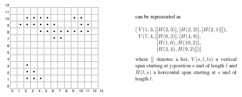
Figure 1: Possible raster set representation for shapes. For a sprite, the same structure is used, but with pixel data added to each horizontal span, possibly compressed with run length encoding.

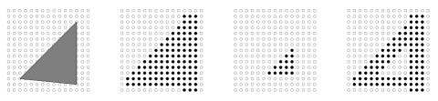
Figure 2: From left to right: A polygon in vector space and its shape, minshape and maxshape as sets of pixels (filled) when using an antialiasing filter with square footprint twice the interpixel spacing.

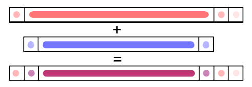
Figure 3: Composing a line of two partially transparent sprites, preserving run-length encoded spans.

Calculating sets for Polygons

Here we give some detail of the calculation of shapes and sprites for a primitive such as the polygon—the process is a little different from traditional polygon rasterization. The shape of a polygon contains every coordinate which will have a not-wholly-transparent value under the rasterizing scheme used to calculate its sprite. This is a simple extension to the standard method for rasterizing filled polygons ([Foley et al. 1996], p92). Scanlines are considered to have a finite width equal to the diameter of the footprint of the antialiasing filter rather than as a zero-width line. The edge list techniques in [Foley et al. 1996] generalize simply.

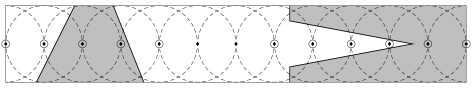
Figure 4: A finite-width scanline and part of a polygon crossing it (shaded), together with the calculated shape scanline (marked as small circles around pixel centres for those pixels included in the shape). The large, dotted overlapping circles are antialiasing filter footprints, though we approximate them with squares for this process. If the left-most pixel here is pixel $0$, $spans(t)$ is {(1–3, 7–12}, $spans(b)$ is {0–3, 7–12} and $covered(e)$ is {0–4,7–12} so the result is {0–4, 7–12}.

Consider a scanline and the list of edges which intersect it, as illustrated in Figure 4. The situation is more complicated than for a zero width scanline. The spans generated by the top and bottom scanline edges may be different, and there may be edges lying partially or wholly within the scanline that must contribute. Let $\mathit{spans}(x)$ be the sequence of spans derived from the list of edge crossings $x$. Let $\mathit{covered}(x)$ be the sequence of spans composed of the coordinates whose associated footprint is intersected by one or more of the current edges $x$ which cross neither the top nor bottom edges. Then, if the current edge list is $e$, the list of crossings at the top edge $t$ and those at the bottom $b$, the spans are $\mathit{spans}(t)\cup\mathit{spans}(b)\cup\mathit{covered}(e)$ where $\cup$ combines touching or overlapping spans to form the minimal set.

When an object is to be rasterized to a sprite, the required shape will have been calculated by the renderer by intersecting the object’s shape with the update shape (the set of pixels in the scene which have been determined to require rendering). The job of the rasterizer, then, is to generate a partial sprite of the same shape. Plain fill types, where the fill colour is constant rather than dependent upon the coordinates of the pixel are treated differently—a run length encoded subspan is generated for runs of pixels which all have no edges intersecting their filter footprint. The antialiased parts around the edges of the polygon are generated as usual.

Figure 3 shows how run length encoding of polygon scanlines is preserved over composition in our spatial representation of sprites. This encoding allows spatial coherence to be preserved when plain shaded possibly-translucent objects are composited over one another.

Hidden Surface Removal Algorithm

A classical painter’s method renderer operates as follows. Objects are dealt with from back-most to front-most. If an object intersects the update rectangle, it is clipped, rendered and composited into a rectangular buffer. In this method, objects contributing nothing to the final image are still drawn, and objects which are partly obscured by ones in front are drawn in their entirety (save for clipping to the update rectangle). This results in many wasted calculations in polygon rasterization, antialiasing and compositing. It also rules out the sensible use of caching techniques for interactive and animation work, since the rasterized objects are very large. One possible approach is to geometrically clip all the objects against one another, but this breaks down in the presence of antialiasing and arbitrary primitives—how can one clip a brush stroke against a point-cloud against a polygon?

To calculate only the parts of an object’s rasterization which will contribute to the final image, the order of rendering is reversed, considering the objects front-most to back-most. Front-to-back rendering is obviously suitable for entirely opaque objects, since the final pixel depends only upon the front-most object affecting it. When objects are partially transparent (or, equivalently, antialiased), the operands to the compositing function may usually be swapped, and the composite calculated starting with the front-most object in the scene. When an object’s rasterization depends upon the objects behind it (such as an object with fill type ‘magnify whatever is below by two, convolving it with a gaussian blur of radius five’), extra work is required—we discuss this in Section 5.

The following description of the rendering process is independent of the implementation of spatial data structures for sprites and shapes, the particular primitives in use and their rasterization methods.

It is convenient to describe the rendering process in terms of a number of fundamental operations on shapes and sprites. An efficient implementation may not create all the intermediate structures suggested by this description.

• $a\wedge b$, the set intersection of two shapes.

• $a\setminus b$, those pixels in shape $a$ which are not in shape $b$.

• $a\vee b$, the set union of two shapes.

• $a\circ b$, which composes sprite $b$ under sprite $a$, returning the composite together with a shape containing those members of $b$ whose analogous pixels in the composite are opaque (and so ‘finished’).

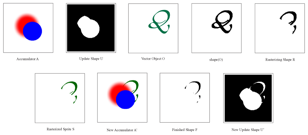
Figure 5: One stage of hidden surface removal front to back. The stages illustrated are repeated for each object in the stack or until the update shape is empty, starting with an update shape which covers the whole update region (a simple rectangle, here).

One stage of this process is illustrated in Figure 5. Call the shape remaining to be updated at this point (the set of pixels not yet in their final form) U, the current object O, and the rendered result A (the accumulator). The function $\mathit{shape}(O)$ calculates the shape of an object $O$ and $\mathit{rasterize}(O,R)$ calculates a partial sprite of $O$ for shape $R$. Proceed as follows:

1. Calculate the intersection between the update shape and the shape of the current object. Call this the rasterizing shape, $\mathrm{R}$.

   $$\mathrm{R}=\mathrm{U}\wedge\textit{shape}(\mathrm{O})$$

2. Rasterize the partial sprite corresponding to $\mathrm{R}$. Call this the object sprite $\mathrm{S}$.

   $$\mathrm{S}=\textit{rasterize}(\mathrm{O},\mathrm{R})$$

3. Compose $\mathrm{S}$ under the accumulator and find the pixels newly finished. A finished pixel is one which is entirely opaque and so cannot be affected by any more objects. Call this shape $\mathrm{F}$. The new accumulator is $\mathrm{A^{\prime}}$.

   $$(\mathrm{A}^{\prime},\mathrm{F})=\mathrm{A}\circ\mathrm{S}$$

4. The new update shape $\mathrm{U}^{\prime}$ is $\mathrm{U}$ with all the newly finished pixels removed.

   $$\mathrm{U}^{\prime}=\mathrm{U}\setminus\mathrm{F}$$

5. Next object with $\mathrm{A}=\mathrm{A}^{\prime},\mathrm{U}=\mathrm{U}^{\prime}$.

After all objects have been processed, the final accumulator sprite $\mathrm{A}^{\prime}$ has a shape which is a subset of the original $\mathrm{U}$. If the output is to be used for rendering to a device which does not have an alpha channel (for instance, a screen), the last object in the scene will be the background (which is everywhere-opaque), so the final result will have the same shape as the original U.

3 Frame-to-frame Coherence

Finding the Update Shape

The rendering model for multiple frames is stateless; it is the job of the program calling the renderer to decide the region which needs to be updated when a change occurs.

Call the set of pixels whose values are considered to have changed the update shape. It depends upon the kind of operation (translation, rotation, deletion etc.) that is performed, and upon properties of the object’s rasterization. When an object undergoes a rotation, for example, the update shape is $a\vee a^{\prime}$ (where $a$ is the old shape, $a^{\prime}$ the new). If, however, the rasterization of that object is independent of the operation (for instance, a plain fill is independent of rotation), the update shape is

$$(\textit{shape}(a)\setminus\textit{minshape}(a^{\prime}))\vee(\textit{shape}(a^{\prime})\setminus\textit{minshape}(a)).$$

The situation is illustrated in Figure 6. Since the shapes are likely to be in a cache (See Section 3), and in any case may be calculated quickly, we expect this to be efficient. There are some circumstances when the update shape is empty even though the scene has changed. For instance if the changes do not affect the current area of the scene viewable on screen, or if the operation is known not to affect the rasterized representation of the scene (for example, ungrouping a group of objects in an interactive illustration package).

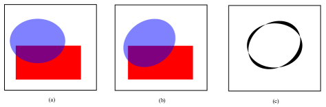
Figure 6: Finding the update shape. The blue oval has been rotated between frames (a) and (b). The update shape is shown in (c). The pixels in the centre of the oval have not changed colour so do not need to be redrawn.

All calculations determining the update shape requiring rasterization in a particular update cycle are implicitly taken to be in intersection with the region of interest, for example the viewport of the current window.

Caching for Interactive Changes

An important side effect of exact hidden surface removal is that the size in memory of an object’s sprite is likely to be smaller due to the use of a spatial data structure and the fact that many objects will only be partially rasterized. This makes caching of part or all of the rasterized data feasible so that, when the scene changes, parts of sprites which have not changed need not be recalculated (when needed as part of a changed composition). The cache can store partial or complete sprites corresponding to the rendered portions of each object. We also store shapes (the sets representing the pixels affected by an object), since these are small and frequently required for the calculations in the hidden surface algorithm.

When a new item is added to the cache, or an object’s partial sprite in the cache extended, one or more cache items may need to be removed to make space. To decide which to remove, the cache items are scored according to various metrics (how recently the item was last used, the time the object took to render, the size in memory of the item, the type of the item – shape or sprite). Often, it is useful to keep previous generations of an object in the cache too—a frequent operation in interactive graphics programs is undo, which should be fast. This also means that, upon zooming in on a part of the scene to inspect it and then returning the original scale, the scene should not have to be recalculated.

It may prove desirable to cache precomposited portions of the image to prevent having to recompose at every update. This works due to depth coherence in successive editing operations. That is, when the user selects an object, it is likely they are about to modify it. One composite sprite for all the objects below the back-most currently-selected object can be made so that as it is (interactively) modified, the re-rendering of the scene is faster.

When the user is interactively, say, rotating an object, the screen must be updated in as near real-time as possible, but the change is not committed to the scene until the mouse button is released. Typically the user can also cancel the interactive operation by pressing the escape key. This scheme has implications for efficient use of the cache. Caching each of the dozens of generations of the sprite of an object which result as the interactive modification is made is unacceptable. Consider how to react when the user has his chosen result and wishes to commit the modification, or wishes to abandon the modification. Upon abandonment, the renderer is called with the update shape $a\vee a^{\prime}$ (where $a$ is the old shape, $a^{\prime}$ the latest of the interactive shapes) and the old scene. Upon commit, the situation is rather more complicated. The new shape and sprite have just been calculated so it is important to avoid recalculating them. This is done by keeping the latest rendered object(s) in the interactive change in a private single-entry cache, moving them into the main cache upon commit.

One of the most common operations when editing a scene is translating an object. Since this operation is often done with the mouse, in a large proportion of cases the translations in $x$ and $y$ will be integers at the current viewing transform. This means the rasterized representation does not change. The geometry of the object changes, but its shape and sprite can just be translated. This does not apply to all objects—filters (see Section 5), for example, can change their rasterized representation based upon their position.

4 Antialiasing and the Problem of
Correlated Mattes

Antialiasing in our system is achieved by integrating over a filter. In our particular implementation, we use a gaussian with a filter footprint width equal to twice the interpixel spacing. Quickly calculating this integration is discussed in [Feibush et al. 1980], [Catmull 1984] and [Duff 1989].

The coverage calculation can be done from the same edge lists which were used to calculate the polygon’s shape. In the simplest case there is just one edge crossing the filter footprint and the volume under the filter may be looked up in a simple table mapping the triple (start point, end point, whether top left corner of footprint is inside or outside) to a value. For reasonable subpixel granularity, this lookup table is small—especially if the fourfold symmetry of the filter is exploited to reduce its size. In our system, the table is just a few hundred bytes for a 16x16 subpixel arrangement. When there are multiple edges, the set of subpixels representing the rasterized edge within the filter footprint is calculated using almost the same system as for calculating shapes given earlier, scaled up so there are multiple spans per pixel. Each subspan can then be looked up in a table mapping (start x, start y, length) to integrated values, which are then summed to find the total contribution. Figure 7 shows an example.

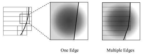
Figure 7: The calculation of antialiasing for polygons using an arbitrary filter. When there is just one edge crossing the filter, a lookup table for filter values based on the two endpoints and inside-outside nature of the top left point is sufficient. When there are multiple edges, we must do the integration in sections, by calculating the shape spans and looking these (start x, start y, length) spans up in another pre-calculated table.

When a shape is rasterized using antialiasing, geometry is exchanged for a single coverage value, and information is lost. This manifests itself when such images are composited with one another, since it is not known how much of the top object obscures the bottom object in each pixel. Porter and Duff [1984] cite one of the worst cases, where the same object is used twice in a compositing expression—it covers itself exactly, but the algorithm blends the colours nonetheless.

Consider Figure 8. Since the red entirely covers the blue, no blue should show through. However, rasterization exchanged geometry for coverage, so the renderer has no information to decide if the blue object is a partially transparent one covering the whole of the pixel, or an opaque one covering part of it. It has no choice but to assume the colours blend. This is known as the problem of correlated mattes. Two other manifestations of this problem are visually disturbing: When a thin line appears to darken as it crosses other lines or itself, and when two abutting polygons appear to have a thin line separating them. Commercial illustration graphics programs have traditionally ignored this problem.

Figure 8: The problem of correlated mattes. A red circle placed exactly over a blue one. The left pair composited as usual; the right pair with proper treatment of correlated mattes.

Any method to solve the problem of correlated mattes will involve a hidden surface algorithm of some kind at certain pixels. Two classic solutions are Carpenter’s A-buffer [Carpenter 1984] and Catmull’s Pixel Integrator [Catmull 1978]. The A-buffer keeps a bitmapped buffer for each pixel affected by polygon edges. The Pixel Integrator analytically clips each polygon to a square surrounding the pixel, and computes each polygon’s visibility exactly.

We should only perform hidden surface removal within individual pixels when it would make a difference to the final composite. It is quite simple to extend our current system with an optional subpixel analysis at the cost of slower rendering: pixels forming part of the maxshape of an object are initially represented by a square matrix of subpixels, covering the footprint of the antialiasing filter in use and stored as a sprite (so space-efficient). When compositing into the accumulator, subpixels are composited with one another in the usual manner. A pixel is finished when all its subpixels are finished. At this stage, the antialiasing filter is applied and the representation of that pixel reverts to normal. This ensures that no more work is done than is required. When all objects have been rendered, any remaining subpixel-represented pixels in the accumulator are normalized. Figure 9 shows an example single pixel accumulator under this system. Note that the shapes are rendered in this subpixel system without antialiasing, so that in the case two identical polygons on top of one another, none of the one beneath would show, as required.

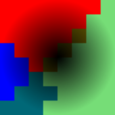
Figure 9: Solution to the problem of correlated mattes by using our usual front-to-back hidden surface removal process within the antialiasing filter footprint of a single pixel. The results are then weighted by the filter to produce a single result, once the pixel is finished.

5 Filters

Sometimes it is useful for the object’s sprite to depend upon the rasterized composite of the objects below it, or for the object to be able to remove objects or change their geometry whilst they lie under it. We call this kind of object a filter. The concept is not new (see, for example, [Bier et al. 1993]), but our system is more general than previous efforts: filters can read from directly underneath themselves, or from other parts of the scene, modifying the result either geometrically or using raster effects. Filters can be made from any type of primitive. For instance, the filter ‘blur the scene below’ requires rendering the scene below normally, and then blurring it to form the sprite of the filter object. The filter type ‘make all objects below have thin lines and transparent fills’ (an outline or wire frame effect) involves modifying the object geometries themselves. A filter has an opacity (plain, or varying) just like any other object, representing the extent to which the filter affects each pixel.

A filter represents an interruption in the usual front-to-back rendering order. Filters complicate the rendering process significantly, especially if we are to preserve the efficiency gains we have seen with simple front-to-back rendering.

A filter consists of:

• The geometry of the filter, which is a primitive of some kind (polygon, brush stroke etc). Only the alpha channel is used, for defining where and to what extent the filter acts. The rasterizations of the filter and base scene will be blended in proportion to this geometry, allowing for correct antialiasing and partially transparent filters.

• The scene function, which takes as input the current scene under the filter and the shape representing the part of the filter’s shape which requires rasterization. It returns a modified scene (perhaps removing, adding or changing objects) whose rasterization will be required before the filter itself can be rasterized, a shape in which that rasterization is required (the reading shape), and a shape representing how much of the filter itself need be rendered (the same or a subset of the input shape).

• The filter function, which performs computation on the sprite returned by the rendering of that part of the scene which is returned by the scene function. For instance, it may blur it.

• The update function, which is used to determine if areas of the filter need updating when some other area of the scene underneath needs updating.

The scene function can, of course, produce a scene with more filters in it, leaving open the possibility of a non-terminating renderer. An interactive graphics program using the renderer must prevent this by construction.

Rendering with Filters

When a filter is encountered, various of the basic set operations defined above are used, together with the filter’s specification, to calculate its sprite and finished pixels. We proceed as follows (letters from Figure 10):

1. Picture (a) is the geometry of the filter. Use the filter’s scene function to find the reading shape (b) and the modified scene.

2. Render (c) the modified scene in the region of the filter which we are rasterizing. Execute the filter function to make (d).

3. Find the pixels (e) in the rendered alpha channel of the filter geometry which are not opaque (this is the maxshape of the filter geometry).

4. Rasterize (f) the original scene in those pixels.

5. Blend (g) the original and filter together, attenuating the filter in proportion to (and the original scene in proportion to the complement of) the alpha channel of the filter geometry and combining them where they overlap using the Porter-Duff ‘plus’ operator. Picture (h) shows this in the context of the eventual, fully-rendered image.

6. The finished pixels for the filter object are all those in the shape of the filter’s sprite, rather than those which are actually opaque as for a non-filter object. This allows filters which take paint away from the canvas to function correctly.

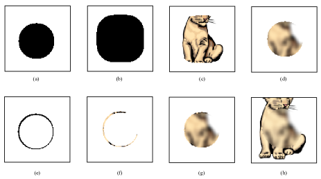
Figure 10: Rendering a filter using its geometry, scene function and filter function. Here the geometry is a polygon, the scene function expands the reading shape (to provide enough data for the blur to be rendered) but does not alter the scene, and the filter function blurs the rendered scene. (a) the shape of the filter’s geometry (b) the reading shape (c) the scene rendered in the reading shape (d) the result of the filter function (e) the pixels where the filtered and unfiltered scenes must be combined (here just the antialiased pixels) (f) the original scene rendered in those pixels (g) sprites (f) and (d) combined using the Porter Duff ’plus’ operator. (h) the whole scene including the filter.

Some Example Filters

Here we describe some filters to illustrate how different scene and filter functions are used. Figures 11 and 14 show the effect of some other filters, with various geometries.

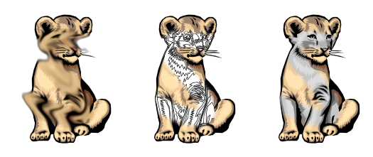
Figure 11: Filter examples, using a brush stroke as the filter geometry. From left to right: smear along the path of the brush stroke, outline (wire frame), monochrome.

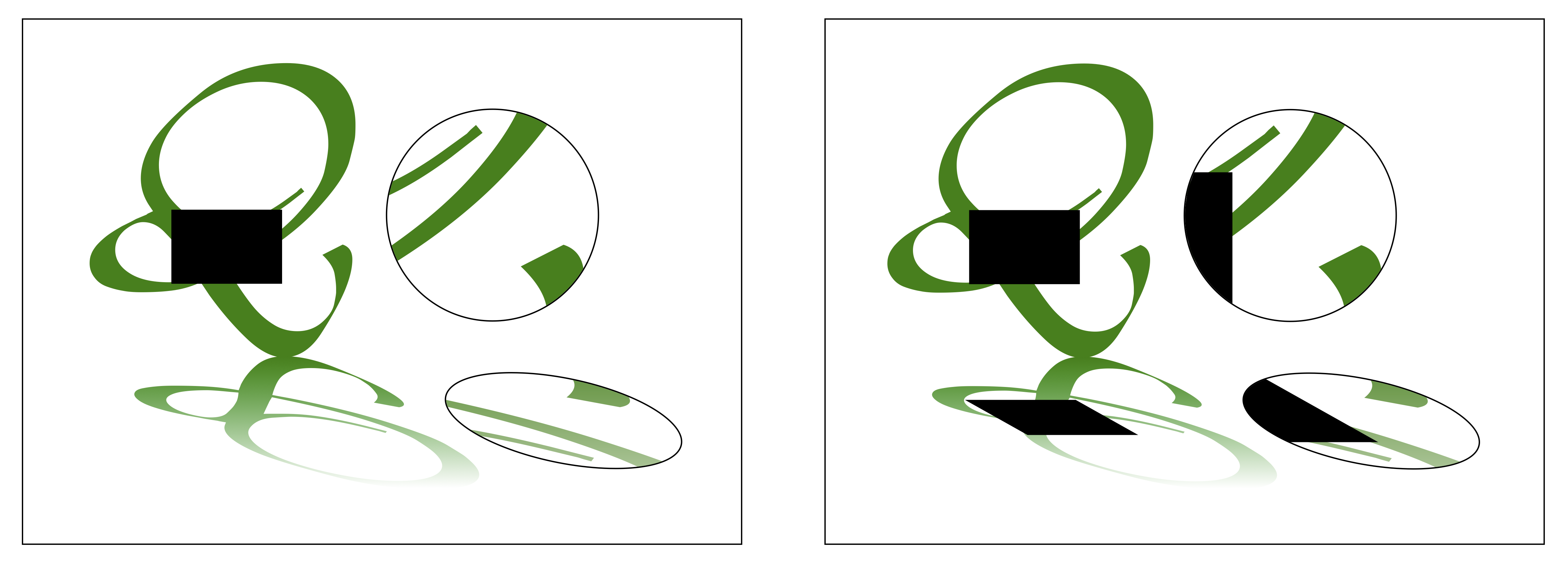
Figure 12: Frame-to-frame coherence in the presence of filters. The left-hand image shows a scene with a zoom filter overlaid with a shadow filter. The black rectangle is the region of the scene requiring update for whatever reason. In the right hand image, the filters’ update functions have been used to propagate the update shape through the scene to determine which other regions have been invalidated by the change.

• Blur To blur the scene in a given area. The scene function returns the scene under the filter unaltered, the reading shape is the shape of the filter geometry convolved with a rectangle of the width and height of the convolution kernel to include the extra pixels required for calculation of a blur. The filter function convolves the sprite by the kernel in the region of the filter geometry, returning a sprite of just those pixels in the original filter geometry.

• Cutting a hole To cut a hole in the entire scene below the filter. The scene function returns the empty scene, the reading shape is the shape of the filter geometry and the filter function is the identity function. A hole can be cut just through one object by returning the scene with that object removed.

• Affine transform To produce a magnify, reflect or similar effect. The scene function applies some affine transform to the scene. The reading shape is unaltered. The filter function is the identity function, or some function such as blurring or tinting, avoiding the needless composition of several filters when one could suffice.

When an object is altered, added or removed from the scene, an initial update shape is calculated using the methods already described. When the scene contains filters, part or all of each filter lying outside this region may need to be recalculated. A simple but inefficient method would be to invalidate the entirety of all filters when a change is made to the scene. However, we wish to preserve the efficiency of exact hidden surface removal over filters, making them almost as efficient as basic shapes. We associate an update function with each filter. The final update shape is given by the composition of the update functions of the filters from the back-most modified object forwards, again taken in intersection with the region of interest. The process is illustrated in Figure 12.

6 Other Primitives

Nothing in our hidden surface algorithm requires that polygons be used—any primitive which can be rendered (i.e. its shape and sprite calculated for a given region) may be used. There is no need to convert them to polygons—they retain their own geometry. Figure 13 shows:

1. A blurred polygon (our renderer allows any object to be blurred).

2. A brush stroke created with the techniques in [Whitted 1983].

3. The subtraction of a brush stroke from a polygon, forming a brush stroke shaped hole in the polygon. Our renderer allows such set operations on any combination of types of geometry, using the same operations to calculate the shape and partial sprite efficiently.

The geometry of a filter may likewise be formed of any primitive or combination of primitives. For example, Figure 11 uses brush stroke shaped filters.

Figure 13: Examples of other primitives: (a) a blurred polygon (b) a brush stroke and (c) a polygon with a brush stroke shaped hole in it. Our system can perform set operations on geometries to build new ones, retaining the efficiencies of their shape and sprite representations.

7 Conclusion

We have presented a method of hidden surface removal for static and moving scenes containing arbitrary primitives and primitive-combiners. We have shown how this works together with updated versions of classic antialiasing and rendering methods to calculate information only when it is required.

Many systems nowadays have either specific accelerated graphics hardware, or multiple CPU cores, or both. Whilst it is always useful to keep a reference software implementation, could this system be implemented wholly inside graphics hardware? To what extent might it be made parallel? More work is required to define the best caching mechanisms based upon empirical observation. There is plenty to be done on efficiency for particular kinds of scenes. It remains to build the renderer into an interactive graphics application for insights into its use in real situations, and to add low level optimisations to complement the algorithmic efficiency already present.

Acknowledgments

The author is indebted to Alvy Ray Smith for his careful and constructive comments on an earlier draft of this work.

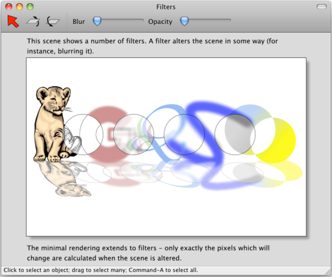
Figure 14: A complete scene shown in our basic editor. The scene shows five objects with four filters in front of them. A final filter on top of the scene reflects, shears and fades the whole scene to form a reflection. The filters (from left to right) are outline (wire frame), colour splitting, blurring and monochrome.

References

- [\citenameBier et al. 1993] Bier, E. A., Stone, M. C., Pier, K., Buxton, W., and DeRose, T. D. 1993. Toolglass and magic lenses: the see-through interface. In Proceedings of the 20th annual conference on Computer graphics and interactive techniques, ACM, New York, NY, USA, SIGGRAPH ’93, 73–80.
- [\citenameBlinn 1998] Blinn, J. 1998. Jim Blinn’s Corner — Dirty Pixels. Computer Graphics and Geometric Modeling. Morgan Kaufmann.
- [\citenameCarpenter 1984] Carpenter, L. 1984. The a-buffer, an antialiased hidden surface method. In Proceedings of the 11th annual conference on Computer graphics and interactive techniques, ACM Press, 103–108.
- [\citenameCatmull 1978] Catmull, E. 1978. A hidden-surface algorithm with anti-aliasing. In Proceedings of the 5th annual conference on Computer graphics and interactive techniques, ACM Press, 6–11.
- [\citenameCatmull 1984] Catmull, E. 1984. An analytic visible surface algorithm for independent pixel processing. SIGGRAPH Comput. Graph. 18, 3 (Jan.), 109–115.
- [\citenameDuff 1989] Duff, T. 1989. Polygon scan conversion by exact convolution. Raster Imaging and Digital Typography, 154–168.
- [\citenameFeibush et al. 1980] Feibush, E. A., Levoy, M., and Cook, R. L. 1980. Synthetic texturing using digital filters. SIGGRAPH Comput. Graph. 14, 3 (July), 294–301.
- [\citenameFekete and Beaudouin-Lafon 1996] Fekete, J.-D., and Beaudouin-Lafon, M. 1996. Using the multi-layer model for building interactive graphical applications. In Proceedings of the 9th annual ACM symposium on User interface software and technology, ACM, New York, NY, USA, UIST ’96, 109–118.
- [\citenameFoley et al. 1996] Foley, J. D., van Dam, A., Feiner, S. K., and Hughes, J. F. 1996. Computer Graphics — Principles and Practice, second ed. The Systems Programming Series. Addison-Wesley.
- [\citenameFroumentin and Willis 1999] Froumentin, M., and Willis, P. 1999. An efficient 2.5D rendering and compositing system. In Proceedings of Eurographics ’99, vol. 18.
- [\citenameGish and Tanner 1992] Gish, W., and Tanner, A. 1992. Hardware antialiasing of lines and polygons. In SI3D ’92: Proceedings of the 1992 symposium on Interactive 3D graphics, ACM Press, 75–86.
- [\citenameO’Rourke 1998] O’Rourke, J. 1998. Computational Geometry in C (Second Edition). Cambridge University Press.
- [\citenamePorter and Duff 1984] Porter, T., and Duff, T. 1984. Compositing digital images. In Proceedings of the 11th annual conference on Computer graphics and interactive techniques, ACM Press, 253–259.
- [\citenameShantzis 1994a] Shantzis, M. A. 1994. A model for efficient and flexible image computing. In SIGGRAPH ’94: Proceedings of the 21st annual conference on Computer graphics and interactive techniques, ACM Press, 147–154.
- [\citenameShantzis 1994b] Shantzis, M. A. 1994. A model for efficient and flexible image computing. In Proceedings of the 21st annual conference on Computer graphics and interactive techniques, ACM Press, 147–154.
- [\citenameSmith 1995a] Smith, A. R. 1995. Alpha and the history of digital compositing. Technical Report 7, Microsoft.
- [\citenameSmith 1995b] Smith, A. R. 1995. Image compositing fundamentals. Technical Report 4, Microsoft.
- [\citenameSmith 1995c] Smith, A. R. 1995. A pixel is not a little square, a pixel is not a little square, a pixel is not a little square! (and a voxel is not a little cube). Technical Report 6, Microsoft.
- [\citenameSmith 1995d] Smith, A. R. 1995. A sprite theory of image computing. Technical Report 5, Microsoft.
- [\citenameSutherland et al. 1974] Sutherland, E. E., Sproull, R. F., and Schumacker, R. A. 1974. A characterization of ten hidden-surface algorithms. ACM Comput. Surv. 6, 1, 1–55.
- [\citenameWallace 1981] Wallace, B. A. 1981. Merging and transformation of raster images for cartoon animation. In Proceedings of the 8th annual conference on Computer graphics and interactive techniques, ACM Press, 253–262.
- [\citenameWhitted 1983] Whitted, T. 1983. Anti-aliased line drawing using brush extrusion. SIGGRAPH Comput. Graph. 17 (July), 151–156.