GatingTree: Pathfinding Analysis of Group-Specific Effects in Cytometry Data

Abstract

Advancements in cytometry technologies have led to a remarkable increase in the number of markers that can be analyzed simultaneously, presenting significant challenges in data analysis. Traditional approaches, such as dimensional reduction techniques and computational clustering, although popular, often face reproducibility challenges due to their heavy reliance on inherent data structures, preventing direct translation of their outputs into gating strategies to be used in downstream experiments. Here we propose the novel Gating Tree methodology, a pathfinding approach that investigates the multidimensional data landscape to unravel group-specific features without the use of dimensional reduction. This method employs novel measures, including enrichment scores and gating entropy, to effectively identify group-specific features within high-dimensional cytometric datasets. Our analysis, applied to both simulated and real cytometric datasets, demonstrates that the Gating Tree not only identifies group-specific features comprehensively but also produces outputs that are immediately usable as gating strategies for unequivocally identifying cell populations. In conclusion, the Gating Tree facilitates a comprehensive analysis of the multidimensional data landscape and provides experimentalists with practical, successive gating strategies that enhance cross-experimental comparisons and downstream analyses such as flow cytometric sorting.

Introduction

Cytometry plays a central role in understanding group-specific effects at the single-cell level. As cytometry technologies advances, increasing number of marker data can be analysed simultaneously, posing significant challenges in data analysis. To manage the high-dimensionality of cytometry data, manual gating alone is becoming not feasible and it is currently a common approach to employ dimensional reduction techniques along with automatic clustering methods[1, 2, 3, 4].

Ensuring reproducibility and robustness in flow cytometric analysis is paramount, as highlighted by Cossarizza et al. [5]. Current methods, which rely heavily on the inherent structure of the dataset, face several challenges. Most notably, dimensional reduction techniques such as Principal Component Analysis (PCA) depend significantly on the dataset’s intrinsic structure, resulting in new, reduced axes that amalgamate multiple markers in various ratios. This issue presents considerable challenges, even for relatively straightforward and linear techniques like PCA and its variants[6]. Furthermore, the application of Uniform Manifold Approximation and Projection (UMAP) in cytometric data analysis can be susceptible to distortions and biases, as recognized in genomic studies [7].

Moreover, popular clustering algorithms like those used in Self-Organizing Map [1] and K-means [2] introduce stochastic elements, which makes it challenging to use their outputs for downstream experiments. Further, clustering methods are sometimes followed by differential analysis to identify group-specific cell clusters within reduced dimensions [8], although this approach is also equally subject to the challenges imposed by dimensional reduction and computational clustering.

Efforts to mitigate these issues have included using reduced data with cluster information to generate actionable gating strategies [9], as well as employing cross-dataset analysis techniques [10, 11]. Nonetheless, these methods still face challenges related to the inherent data structure within each dataset. We have also extensively worked on gene expression data and flow cytometric data, using various methods for dimensional reduction and clustering [12, 6, 2, 13], and have found significant challenges in translating data from dimensional reduction or clustering into wider research contexts.

Thus, there is a pressing need for new methodologies that can elucidate group-specific features within multidimensional marker data without relying on dimensional reduction or computational clustering with a stochastic element. Overcoming the challenges posed by the expansion of combinatorial numbers with increased marker use could provide significant benefits to the research community in academia and industry, offering new avenues for automating flow cytometric data analysis.

In this study, we introduce GatingTree, a novel methodology employing a pathfinding approach to high-dimensional data, which offers immediately and directly applicable gating strategies for identifying group-specific features without the use of dimensional reduction. We examine whether combinatorial data expansion truly occurs in real-world data and demonstrate that it is manageable due to limitations in real-world settings. By developing methods for GatingTree, we analyze multiple simulated and non-simulated real-world datasets to demonstrate the utility of the methodology.

Cytometry Analysis in Real-world

The number of cells that can be analyzed per experiment is significantly constrained in real-world settings and is typically less than 1 million cells per sample, primarily due to the following limitations.

Sample Availability and Antibody Staining: The cell number of single cell suspension for cytometry samples ranges from $10^{4}$ up to $10^{7}$ cells. The number of lymphocytes available from murine lymphoid organs is typically millions per organ. Tissue-infiltrating immune cells are rarer, generally ranging from 100 to 400 cells per $mm^{3}$ of tumor tissue [14], resulting in total counts from $10^{4}-10^{6}$ per sample. Human peripheral blood typically yields approximately 1 million peripheral blood mononuclear cells (PBMCs) per mL [15].

Standard antibody staining practices involve using 96-well plates to process cell samples. Typically, 1 million cells are stained per sample [16, 17], although this number may increase to up to 10 million for analyses focusing on rare cells [18].

Data Acquisition Rate: Mass cytometry is commonly performed at rates up to 500 events per second [19], while several thousand events per second are achievable with flow cytometry. The rate around 2,000 events per second is considered ideal in our lab to optimize data quality and avoid blockages in the flow system.

Timeline of Experiment and Replicates: Sample preparation and instrument calibration can take several hours, with only about 4 hours typically available for sample acquisition. Additionally, it is common to analyze multiple cytometry samples from each biological material. In immunology experiments, for instance, various organs such as tumor-infiltrating lymphocytes, spleen, and superficial lymph nodes are often analyzed. In addition, multiple antibody panels like myeloid and lymphocyte panels may be used.

Target Cell Population: In most cases, not all cell populations are analyzed in a single experiment. For example, T cell biologists focus on detailed features of T cells, but not typically myeloid cells. The prevalence of T cells in samples can vary depending on the origin of samples cell viability, and the number of debris, but this can be between 5 - 30%.

Example:

In a typical immunology experiment intended to generate a dataset with 10 replicates for two groups and two organs, the total time allocated for analysis per flow cytometry sample is approximately 6 minutes within a 4-hour window. Given an acquisition rate of 2,000 events per second, the number of target cells that can be analyzed per sample is $7.2\times 10^{5}\times p,$where $p$ represents the prevalence of the target cell population (ranging from 0 to 1). Consequently, aiming to analyze T cells, the upper limit of target cell numbers per sample is estimated to be about $2\times 10^{5}$ cells only.

Cell Number Exhaustion in Combinatorial Marker Gates

Given each marker is employed to delineate a minority population, multiple successive gates exponentially decreases the cell number, as more markers are integrated (designated as cell number exhaustion).

Assuming a minimum threshold of 25 cells per sample in a gate for robust analysis, a mass cytometry dataset from Krieg et al.[20], which utilized 24 labeled antibodies and analyzed thousands of cells per sample, the majority of gated fractions – designated as nodes – showed a cell number exhaustion at the depth 6, i.e. the combination of six markers (Figure 1 A). In this context, a node refers to a subset of cells that share specific marker combinations. Similarly, a flow cytometric dataset from Hassan et al.[21], which used 11 labeled antibodies, showed optimal node abundance at 5 marker combinations (Figure 1 B). The number of available nodes at each depth peaked at the depth 9 for [20]

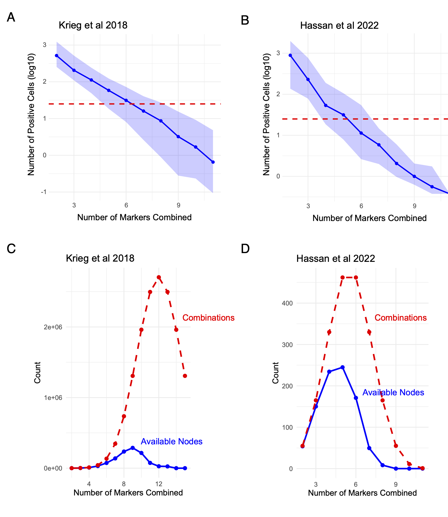
Figure 1: Effects of Cell Number Exhaustion on Available Combinatorial Gate Numbers. (A, B) Logarithmic plot of the number of positive cells against the number of markers combined for (A) Krieg et al. 2018, which analyzed 25 markers, and (B) Hassan et al. 2022, which analyzed 11 markers. The dashed red line indicates the threshold below which nodes (i.e. gates) are considered exhausted (cell number = 25). (C, D) Comparison of combinations and available nodes for (C) Krieg et al. 2018 [20] and (D) Hassan et al. 2022 [21]. The solid blue line represents the count of available nodes, and the dashed red line indicates the number of all marker combinations.

Aim of the Proposed Methodology

The primary goal of this novel methodology is to analyze high-dimensional cytometry datasets for two-group comparisons, facilitating the identification of group-specific cell clusters that are compatible with downstream experimental procedures, including flow cytometric sorting. This objective is underpinned by the following key requirements:

1. The methodology should generate gating strategies that can be directly applied to downstream experiments, ensuring practical applicability and seamless integration into laboratory workflows.

2. It will eschew methods that rely heavily on the underlying data structure, such as dimensional reduction techniques, to preserve the natural variability and integrity of the data.

3. It must efficiently handle the combinatorial complexity inherent in datasets with numerous markers, ensuring that the analysis remains computationally feasible and robust.

Investigation of Multidimensional Marker Space and Construction of Gating Tree

Our aim has led to the development of a novel approach for constructing Gating Tree, which represents a series of gating strategies, through successively investigating the multidimensional marker space within cytometry data. This methodology employs a metaphorical Turtle to systematically navigate the landscape of the multidimensional marker space. Each location within this space, referred to as a node, is defined by a specific combination of marker states and include cells from all samples that have the marker states. The ’height’ at each node represents the degree of enrichment of cells in the experimental group relative to the control group.

The expression of marker is categorised into positive and negative, or high and low. The advantage of the simple categorisation is that it is unequivocally determined, more robust and efficient than arbitrary polygon or oval gating. This leads to each marker having three possible states, including an unassigned state (i.e., when the marker is not used), thereby structuring the space as a 3-dimensional hypercube with $n$ dimensions. The total number of possible locations (or nodes), including the origin, is thus given by $N=3^{n}$. Thus, the Turtle still needs to fight with the expansion of exponential numbers by choosing meaningful routes only based on the landscape investigation.

The Turtle’s journey begins in a state of neutrality ($0$) across all marker axes. It may then select any marker and advance to one of two positions: positive ($+1$) or negative ($-1$). Transitioning from the neutral state to either positive or negative, or from one marker state to another, constitutes a unit of movement. The Turtle’s path across these markers forms a series of successive gating strategies, evolving into a branching structure, which is designated as Gating Tree.

Each node within the Gating Tree represents a decision point where the Turtle evaluates the landscape of the multidimensional marker space. As illustrated in Figure 1 panels A and B, the distribution of cells along the x-axis is notably left-skewed, prompting the Turtle to commence its exploration from nodes that are directly adjacent to the origin—these nodes represent all possible single marker states, both positive and negative. The Turtle’s subsequent movements are determined by the following clearly defined node rules:

Rule 1: Starting from each available marker, the Turtle investigates the landscape by moving towards directions where cells from the experimental group are significantly enriched compared to the control group. This navigational strategy is quantified and guided by the development of a new metric, the Enrichment Score. Rule 2: To minimize the influence of outliers, the Turtle avoids directions that lead to a reduction in informative content. This principle of seeking paths with maximal information gain sets the foundation for the introduction of a novel metric we term Gating Entropy, which is a variant of Conditional Entropy. Rule 3: The Turtle will not crawl to the nodes that do not have cells more than a pre-determined threshold.

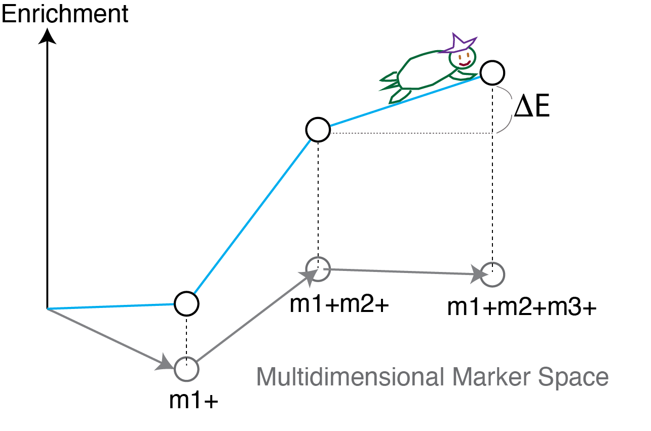
Figure 2: Schematic Representation of Turtle’s Exploration in Multidimensional Marker Space. The z-axis represents the Enrichment Score, while the x-y plane symbolizes the multidimensional marker space itself. The Turtle strategically navigates this space, aiming to always ’climb’ the landscape. The differential ’heights’ between two nodes provide the change in enrichment score, denoted by $\Delta E$, which quantifies the relative increase in enrichment between the nodes.

Should the node rules be satisfied, the Turtle may crawl to multiple nodes from a single node, always ’climbing’ to increase the enrichment score (Figure 2). In doing so, the Turtle’s paths will evolve into the successive gating strategies that identify experimental group-specific effects. This recursive application of the node rules continues until no additional nodes meet the criteria, at which point the final node in the path serves as a leaf in the Gating Tree.

Successive Gating Strategy Formalized as Conditional Gating

Each marker $m_{k}$ defines a basic gate that determines the logical status (e.g., positive or negative) of each cell. During the pathfinding process, the Turtle incrementally constructs a gating path by adding one marker gate at a time to the existing set of gates. Specifically, a single unit move of the Turtle extends the current gate $g_{i}$, which comprises the markers $\{m_{1},m_{2},\ldots,m_{i}\}$, by incorporating the next marker $m_{i+1}$.

This results in a new gate $g_{i+1}$, effectively formed by the logical AND operation between $g_{i}$ and $m_{i+1}$. Consequently, the probability of a cell passing through gate $g_{i+1}$ is determined using the product rule of probability:

$$P(g_{i+1})=P(g_{i}\land m_{i+1})=P(m_{i+1}|g_{i})\times P(g_{i})$$

This formula underscores the conditional dependence of $g_{i+1}$ on $g_{i}$ and the sequential nature of the gating strategy employed by the Turtle.

Enrichment Score and Differential Enrichment

To compare gating performance between an experimental group and a control group, we define the Enrichment score $E(g_{i})$ as:

$$E(g_{i})=\log\left(\frac{p_{e}(g_{i})}{p_{c}(g_{i})}\right)$$

Here, $p_{e}(g_{i})$ and $p_{c}(g_{i})$ are the means of the percentages of cells that satisfy gate $g_{i}$ across all samples in the experimental and control groups, respectively.

Using the product rule of conditional probability (see Methods), the differential Enrichment score from the current gate $g_{i}$ to the next gate $g_{i+1}$ is defined as:

$$\Delta E(g_{i+1})=\log\left(\frac{p_{e}(g_{i+1})}{p_{c}(g_{i+1})}\right)-\log\left(\frac{p_{e}(g_{i})}{p_{c}(g_{i})}\right)=\log\left(\frac{p_{e}(m_{i+1}|g_{i})}{p_{c}(m_{i+1}|g_{i})}\right)$$

This represents the log ratio of the conditional probabilities for the marker $m_{i+1}$ between the experimental and control groups, given the previous gating step $g_{i}$. By systematically investigating the distribution of $\Delta E$ for each marker given various available gates, $\Delta E$ can be used to identify effective markers to identify the experimental-group specific effects.

Gating Entropy and Information Gain

To mitigate the effects of outliers on the enrichment score and to assess the discriminative power of gating conditions, we introduce Gating Entropy, a variant of conditional entropy. This metric quantifies the effectiveness of a gating condition in distinguishing between the Treatment and Control groups based on the percentages of marker-positive cells in each sample.

Conceptual Overview:

At each node of the gating tree, the percentages of cells that meet the gating condition (e.g., being positive or negative for a specific marker combination) are calculated for all samples. The key idea is to evaluate whether these percentages can effectively separate the two groups. Gating entropy measures the uncertainty in correctly classifying samples into their respective groups based on the gating condition.

Calculation of Gating Entropy:

1. Classification of Samples:

1. Calculate the global mean percentage $\mu_{\text{global}}$ of marker-positive cells across all samples:

   $$\mu_{\text{global}}=\frac{n_{\text{Treatment}}\times\overline{p}_{\text{Treatment}}+n_{\text{Control}}\times\overline{p}_{\text{Control}}}{n_{\text{Treatment}}+n_{\text{Control}}},$$

   where:

   • $n_{\text{Treatment}}$ and $n_{\text{Control}}$ are the numbers of samples in the Treatment and Control groups,

   • $\overline{p}_{\text{Treatment}}$ and $\overline{p}_{\text{Control}}$ are the average percentages of marker-positive cells in each group.

2. Classify each sample as ’High’ if its percentage $p_{i}$ exceeds $\mu_{\text{global}}$, or ’Low’ otherwise:

   $$\text{Class}_{i}=\begin{cases}\text{'High'},&\text{if }p_{i}>\mu_{\text{global}},\\ \text{'Low'},&\text{if }p_{i}\leq\mu_{\text{global}},\end{cases}$$

   where $p_{i}$ is the percentage of marker-positive cells for sample $i$.

2. Computing Conditional Entropy:

The gating entropy $H(\text{Group}|\text{Class})$ is calculated using the conditional entropy formula:

$$H(\text{Group}|\text{Class})=-\sum_{x\in\{\text{High},\text{Low}\}}P(x)\sum_{y\in\{\text{Treatment},\text{Control}\}}P(y|x)\log_{2}P(y|x),$$ (1)

where:

• $P(x)$ is the proportion of samples classified as ’High’ or ’Low’,

• $P(y|x)$ is the probability of a sample belonging to group $y$ (Treatment or Control) given its classification $x$ (High or Low).

3. Interpretation:

• A gating entropy of 0 indicates perfect separation, where each classification (’High’ or ’Low’) exclusively contains samples from one group.

• An entropy closer to 1 indicates that the gating condition does not effectively distinguish between the groups.

Information Gain:

Information gain quantifies the improvement in group classification when moving from one gating condition to the next in the gating tree. It is defined as the reduction in gating entropy achieved by applying an additional gating condition.

For a gating strategy $g_{i+1}$ following the current gating $g_{i}$, the information gain $\Delta I$ is calculated as:

$$\Delta I=H(\text{Group}|g_{i})-H(\text{Group}|g_{i+1}),$$

where:

• $H(\text{Group}|g_{i})$ is the gating entropy at the current node,

• $H(\text{Group}|g_{i+1})$ is the gating entropy at the next node after applying the additional gating condition.

A higher information gain indicates that the additional gating condition significantly improves the distinction between the Treatment and Control groups. By utilizing gating entropy and information gain, we can systematically evaluate and select gating conditions that most effectively discriminate between groups.

Algorithm for Gating Tree Construction

The Turtle will start its journey at the origin, which becomes the Root Node. Next, the Turtle moves to all first-level child nodes, each of which represents one of all available markers, including both positive and negative states. The Turtle investigates the cell number, gating entropy, and enrichment score at each node. Then, the Turtle starts a recursive journey, in which the Turtle crawl to the next nodes that satisfy $\Delta E(g_{i+1})>\epsilon\land\Delta I(Y\mid g_{i+1})\geq 0\land n_{i+1}>n_{threshold}$ (Algorithm 1). Note that the Turtle always investigates the number of cells at the next node $g_{i+1}$, $n_{i+1}$ and do not proceed with nodes that does not contain the minimal number of cells.

Algorithm 1 Decision-Making Process of the Turtle for Navigating Nodes

1:Root Rule: Move to all available first-level child nodes.

2:General Node Rule::

3:for each node $g_{i}$ starting from $g_{1}$ do

4:     Calculate $E(g_{i})$ and $H(Y|g_{i})$

5:     for each potential next node $g_{i+1}$ do

6:         Calculate $E(g_{i+1})$, $H(Y|g_{i+1})$, and $n_{i+1}$

7:         Calculate $\Delta E(g_{i+1})$ and $\Delta I(Y|g_{i+1})$

8:         if $\Delta E(g_{i+1})>\epsilon$ and $\Delta I(Y|g_{i+1})\geq 0$ and $n_{i+1}>n_{\text{threshold}}$ then

9:              Move Turtle to node $g_{i+1}$

10:              Update current node to $g_{i+1}$

11:         else

12:              Continue checking other potential nodes

13:         end if

14:     end for

15:     if no nodes satisfy the conditions then

16:         Stop movement and make the current node a Leaf node

17:     end if

18:end for

Specifically, if all available nodes exhibit lower enrichment scores than the current node, the latter is labeled as a ’Leaf’ and also as ’Peak,’ as this is crucial for understanding the geography of the data.

All paths the Turtle traverses will constitute a tree structure, defined as a GatingTree object (Figure 3). In the implementation, GatingTree is realized as a list object in the R environment. As shown in Figure 3, the GatingTree object maintains a tree structure, and the ’Children’ slot includes direct descendant nodes. The ’NodeData’ slot is implemented as multiple slots in the actual implementation, including slots for enrichment score, entropy, cell indices, the leaf status, and the full path at each node.

Pruning of Gating Tree and Node Statistics

The complexity of the Gating Tree constructed depends on the cytometry dataset, particularly the effect size and statistical power to detect group-specific effects. In datasets with considerable differences between groups, users may wish to focus on the most salient features by removing redundancies and prioritizing more abundant cell populations over their minor subsets. To facilitate this, the Gating Tree is designed to be prunable. Users can prune the constructed Gating Tree by setting thresholds for maximum entropy, minimum enrichment score, and average cell percentage.

After pruning, nodes can be extracted from Gating Tree and subjected to statistical test. The current implementation uses Mann Whitney test with p-value adjustment for multiple comparison.

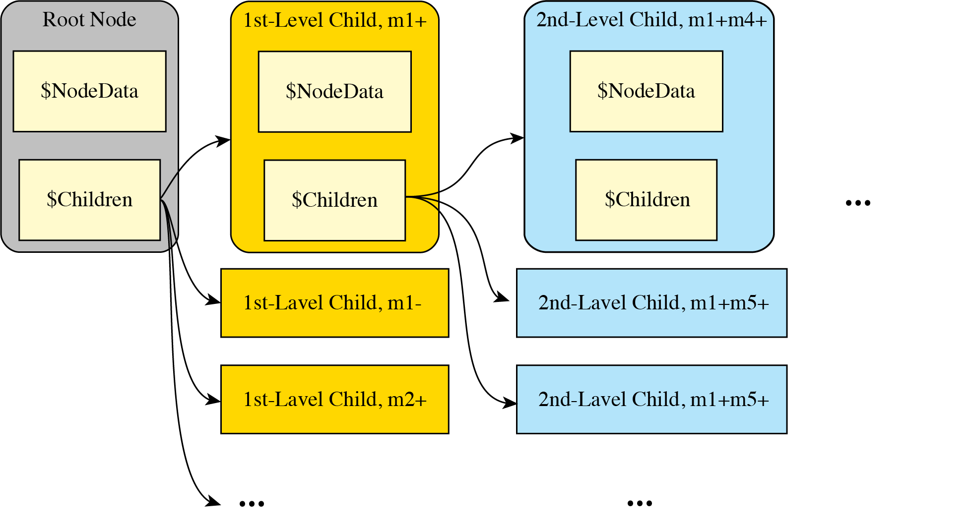
Figure 3: Schematic Representation of the Structure of GatingTree Object. The figure simplifies the structure of the GatingTree object, showing that each node carries the slot NodeData, which in the actual implementation is composed of multiple slots including those for enrichment score, entropy, cell indices, leaf and peak statuses, and the full path at each node, but not including expression data. Child nodes are included in the slot Children.

Example 1: Simulated Data Using a Mixed Gaussian Model

Simulated flow cytometric data were generated using a mixed Gaussian model (see Methods) and analyzed using the proposed Gating Tree method along with FlowSOM (FSOM)-based clustering. As shown in Figure 4A, the number of cells within the gate $m7+m8+m9+$ was increased by various ratios through random injections, with all cells in this gate designated as true cells. Receiver Operator Characteristic (ROC) analysis revealed that the Gating Tree method outperformed FSOM-based clustering (Figure 4B). The Precision-Recall Curve analysis demonstrated that both methods performed well (Figure 4C).

As anticipated, $\Delta E$ values were significantly higher for the markers m7+, m8+, and m9+, indicating that the inclusion of each marker in the gating strategy substantially enhanced the enrichment score of the nodes (Figure 4D).

Figure 4D shows the Gating Tree constructed by the analysis. The figure should be read as displaying successive gates from the origin (Root). The first child node, m7+, has an enrichment of 0.05. Its child nodes, m8+ and m9+, have the gating strategies m7+m8+ and m7+m9+, respectively. The enrichment score is indicated by the size of the node, and the gating entropy is shown by the color of the node. Thus, the node m9+, following m8+ and m7+ (i.e., m7+m8+m9+), has the highest enrichment score of 1.00 and the lowest entropy, 0.0. In addition, combination gates using two of the three markers—m7+, m8+, and m9+—demonstrate a moderate degree of enrichment, further underscoring the capability of Gating Tree analysis to provide comprehensive insights into the dataset.

The constructed Gating Tree visualizes the successive gating strategies as a tree structure, equipped with visual aids for enrichment score and entropy, enabling users to identify critical marker combinations effectively (Figure 4E).

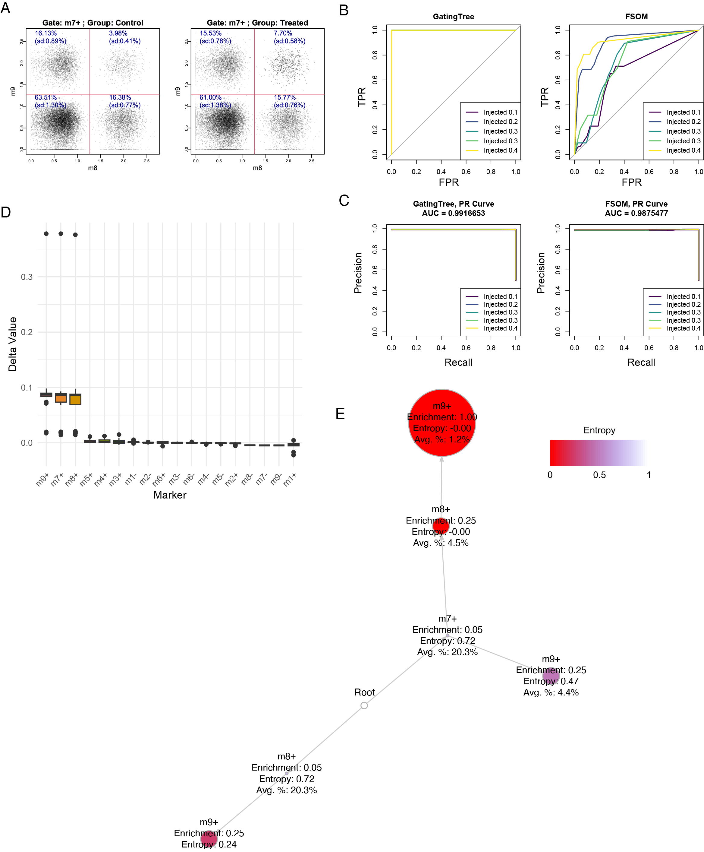
Figure 4: GatingTree Analysis of Simulated Flow Cytometric Data using a Mixed Gaussian Model. Nine-dimensional data were generated for two groups, each with 10 replicates. The experimental group contained a higher number of m7+m8+m9+ cells, randomly enhanced by one of the ratios 0.1, 0.2, 0.3, or 0.4. (A) A two-dimensional flow cytometric plot showing the increased percentage of m7+m8+m9+ cells in the experimental group. (B, C) ROC and Precision-Recall Curves for GatingTree and FlowSOM. (D) Boxplot of $\Delta E$ for each marker, with an injection ratio of 0.4. (E) GatingTree plot, showing the hierarchical structure and the enrichment and entropy of each node by the size and color of each node. Avg. % indicates the mean percentage of cells in the gate among all available cells.

Example 2: A Hybrid Mass Cytometry Dataset with Simulated Cells

Next, we analyzed a hybrid mass cytometry dataset from bone marrow cells with spiked-in leukemia cells (Acute Myeloid Leukemia, AML) with five replicates (AML-sim, [22]). Three datasets were analyzed with spiked-in cells at concentrations of 5%, 1%, and 0.1%.

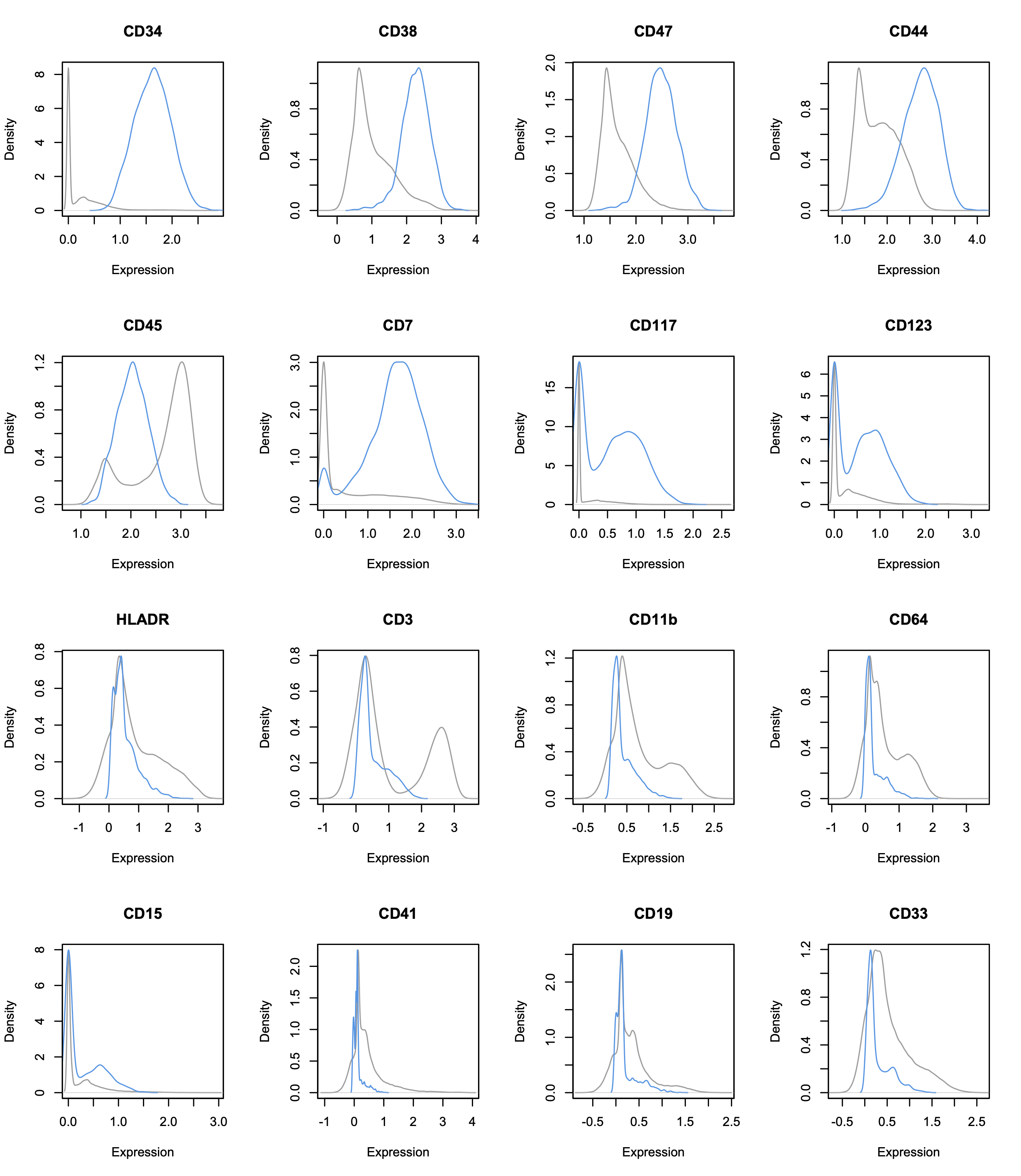
Figure 16: Supplementary Figure S1. The expression profiles of spiked-in leukemia cells (blue) and baseline bone marrow cells (gray) in AML sim data.

ROC and Precision-Recall Curve analyses indicated that the Gating Tree method exhibited robust and high performance (Figure 5). $\Delta E$ analysis identified markers CD34⁺, CD117⁺, CD7⁺, CD123⁺, CD47⁺, and CD38⁺ as having notably high values. Importantly, the expression of these markers was highly upregulated in the injected AML cells (Figure 16), which supports the effectiveness of the $\Delta E$ approach.

The dataset included 14 markers. However, all nodes showed a cell number exhaustion at the third-level children and therefore the output data contained second-level children. The construction of the GatingTree object required approximately 30 seconds. Interestingly, the first-level child nodes with a single-positive marker state—specifically those with a single-negative marker state for CD34^-, CD47^-, CD7^-, and CD38^- —experienced a peak during the Gating Tree construction. This indicated that no additional markers improved enrichment score, suggesting that experimental group-specific cells were enriched only in locations with the positivity for one of the four markers.

To demonstrate the effectiveness of Gating Tree Pruning, Figures 5D and E display the Gating Tree before and after pruning, respectively. By pruning the Gating Tree under conditions where gating entropy is less than 0.5 and enrichment score is greater than 0.5, and by removing all redundant branches, the pruned Gating Tree effectively highlights the utility of key markers with high $\Delta E$ values. It identifies CD34⁺ as a crucial hub gate for enriching AML cells, particularly through the utilization of CD7⁺, CD47⁺, and CD38⁺ markers, demonstrated high enrichment scores and low entropy values (Figure 5D), pinpointing the optimal marker combinations CD34⁺CD7⁺, CD34⁺CD47⁺, and CD34⁺CD38⁺.

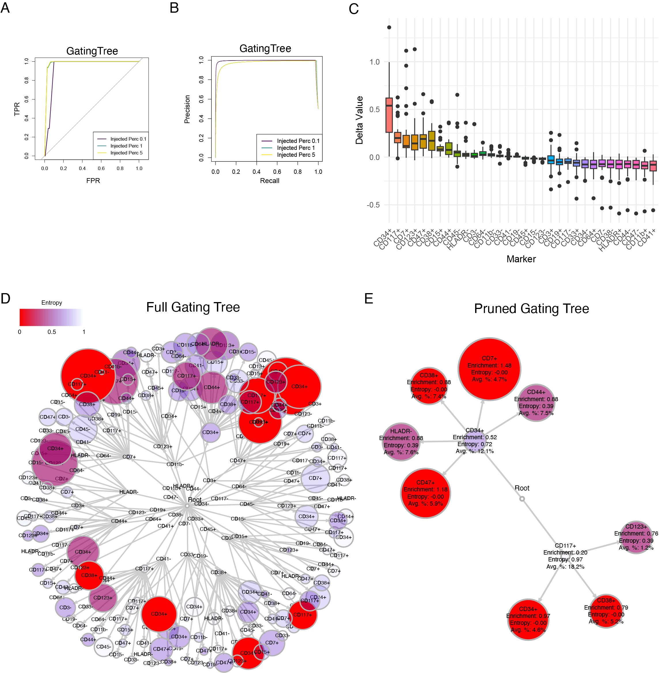
Figure 5: Gating TreeAnalysis of Hybrid Mass Cytometry Data. The dataset is from bone marrow cell data with spiked-in leukemic cells (AML sim, [22]). has 16 marker variables and two groups with 5 replicates. Leukemic cells were injected with 0.1, 1, 5 percentage of total cells. (A, B) (A) ROC and (B) Precision-Recall Curves for GatingTree. (C) Boxplot of $\Delta E$ for each marker, with an injection ratio of 5%. (D) Gating Tree plot, showing the hierarchical structure and the enrichment and entropy of each node by the size and color of each node. Avg. % indicates the mean percentage of cells in the gate among all available cells.(E) Pruned Gating Tree plot with the conditions, gating entropy $<0.5$ and enrichment score $>0.5$.

Example 3: Real-world Dataset from Cancer Patients Under Immune Blockade Therapy

Lastly, we analyzed a real-world flow cytometric dataset from cancer patients under immune checkpoint blockade therapy using anti-PD1 antibody [20]. The dataset analyzed peripheral blood mononuclear cells (PBMCs) of a cohort of 20 patients with malignant melanoma, which were classified into ’Responders (R)’ ($n=9$) and ’Nonresponders (NR)’ group ($n=11$) depending on their clinical response to the therapy. The mass cytometry data analyzed 24 markers.

The small number of samples, the relatively large number of markers analyzed, and the ambitious research aim to identify the phenotype that is correlated to the clinical response, which effect size is presumably small, suggested challenges in data analysis. Still, we decided to use this valuable cytometry dataset to demonstrate the possible strategies for the use of Gating Tree in a real research context.

Gating Tree analysis identified 64,663 nodes as non-exhausted among 213,052 possible nodes up to depth 4. $\Delta E$ analysis showed moderate contributions of markers including CD11b, CD14, ICAM1, CD33, CD16, CD66b, CD123, CD86, and PDL1, with mean $\Delta E$ values greater than 0.25 (Figure 6A). This suggested a significant challenge in pinpointing single markers responsible for the clinical response. By pruning the Gating Tree under the conditions that the gating entropy is less than 0.7 and the enrichment score is greater than 1, top nodes were highlighted as shown in Figure 6B. In this analysis, the markers CD11c⁺ and CD33⁺ are notably used as hub markers, and the markers PDL1⁺, ICAM1⁺, and CD86⁺ increased the enrichment score and decreased entropy values. These findings overall support the increase of unique mature dendritic cells and monocytes with uniquely upregulated PDL1 expression in the responder group. The top-ranked node, CD11c⁺ICAM1⁺PDL1⁺ cells, showed a significant increase in the responder group (Figure 6C and D).

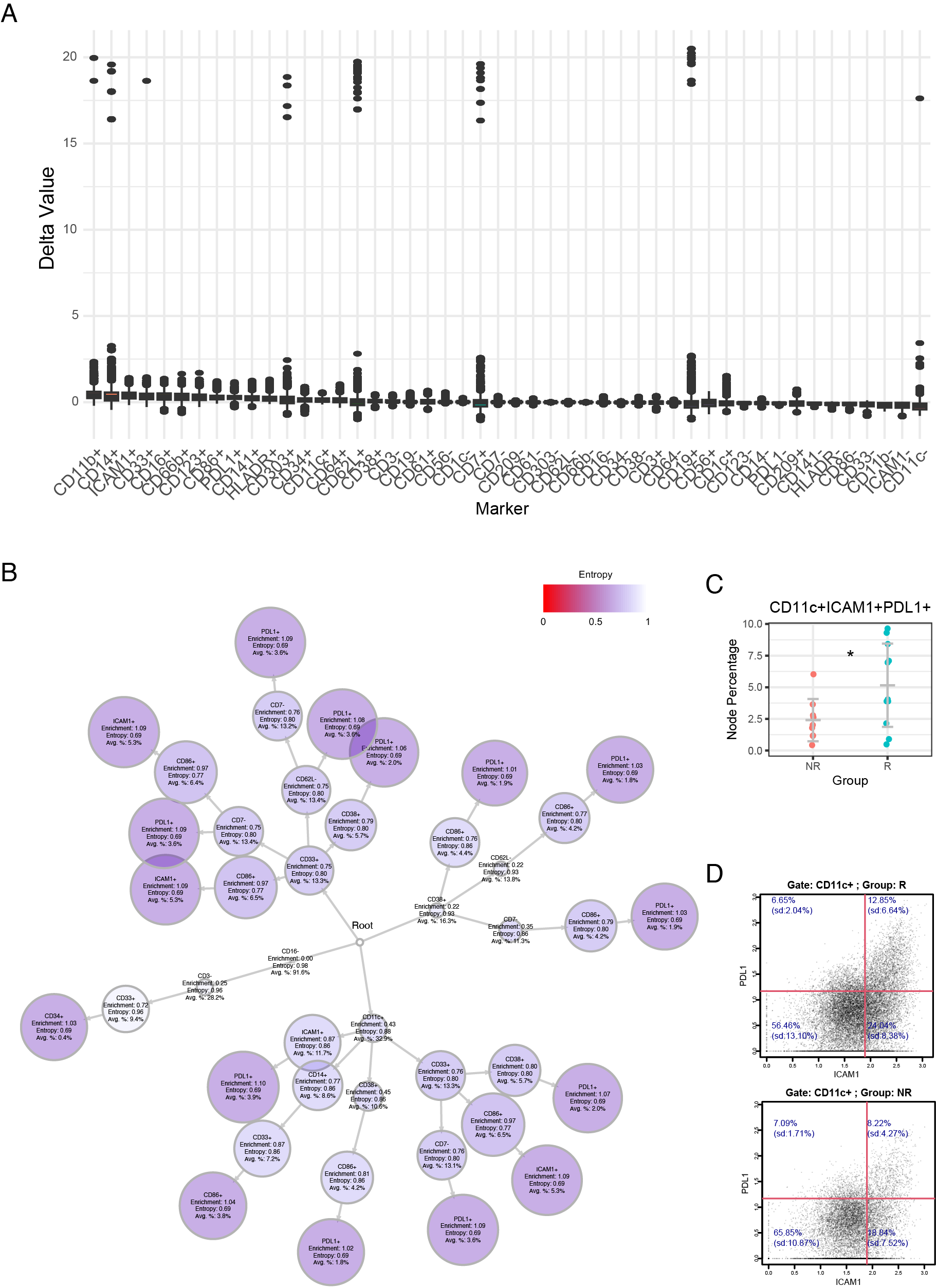
Figure 6: Gating Tree Analysis of Cytometry Data from patients under PD1 blockade. The dataset compares responder and nonresponder patients to PD1 blockade [20, 22]. (A, B) Boxplot of $\Delta E$ showing all data points (A) and a magnified view (B). (C) Gating Tree Analysis of the PD1 dataset. The tree was pruned to identify the most remarkable and distinct nodes (gates). (D) Percentage of individual samples within one of the top gates is shown for a demonstration purpose. Asterisk indicates $p<0.05$ by Mann-Whitney test.

Implementation

GatingTree is implemented as an R package utilizing the S4 object system, FlowObject, which facilitates a comprehensive workflow encompassing data initialization, preprocessing, execution of GatingTree analyses, and data visualization.

Data Structure

All data are stored and systematically analyzed within FlowObject in the GatingTree package (Figure 7A and B).

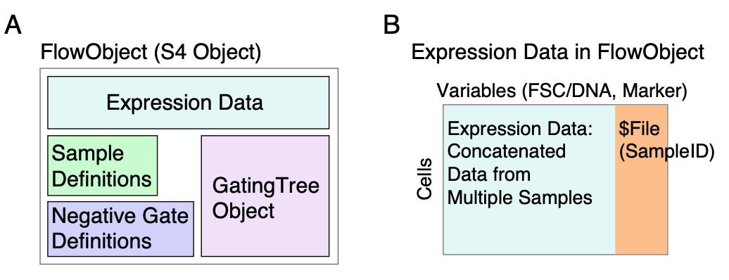
Figure 7: Structure of FlowObject and its components. (A) Slots in FlowObject include Expression Data, Sample Definitions, which define sample grouping, Negative Gate Definitions, and GatingTree Object. (B) Expression Data in FlowObject is created by concatenating expression data from all samples. The column ‘File‘ identifies sample origins.

Overview of Workflow

Immediately after initialization by CreateFlowObject, FlowObject includes expression data and sample definitions. This is followed by data transformation, employing a logarithmic transformation. DefineNegatives allows users to define negative gates. Subsequently, the GatingTree package offers an option to moderate extreme negative values by enforcing a normal distribution within the negative (autofluorescence) range (NormAF). This adjustment facilitates effective visualization of histograms and 2D plots, while preserving the quantitative accuracy of logarithmic transformation for positive cells.

Upon completing data initialization, transformation, and negative threshold definitions for all markers, the function CreateGatingTreeObject can be applied to FlowObject, creating a GatingTree object, which is a list object, within FlowObject (Figure 8). This will be followed by visualization of the constructed GatingTree and enrichment score analysis to determine the impact of each marker state on the enrichment score.

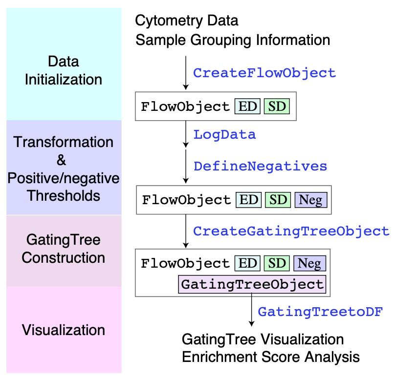
Figure 8: Overview of the workflow depicting the significance of each function at each step of data analysis, clarifying the sequence of function applications. ED: expression data; SD: sample definitions; Neg: negative gate definitions.

Analyzing Cytometry Data with GatingTree

This section demonstrates how to analyze cytometry data using the GatingTree package in R. We will walk through the entire workflow, including data loading, preprocessing, creating a FlowObject, data transformation, defining positive/negative thresholds interactively, performing gating tree analysis, and visualizing the results.

This example shows the analysis of the hybrid mass cytometry dataset constructed by spiking a small percentage of Acute Myeloid Leukemia (AML) cells into healthy bone marrow cells [22], as analyzed in (Figure 5).

1. Creating a FlowObject and Applying Data Transformation

Using CreateFlowObject, construction of FlowObject can be done by two approaches (Figure 9). First, expression data and sample definitions, each as data frame object can be used to create a FlowObject.

library(GatingTree)
x <- CreateFlowObject(Data = Data, sampledef = sampledef,
Ψ experiment_name = ’AML_sim’)

Alternatively, expression data of each sample can be prepared as a csv file, and the entire set of sample data as multiple csv files can be imported, creating a FlowObject. Using the second approach, sample definitions can be imported by the function SampleDef.

#library(GatingTree)
#Assuming that all csv files are included in the working directory,
x <- CreateFlowObject()

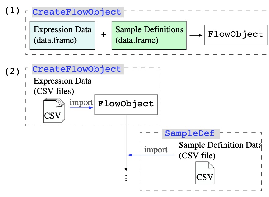
Figure 9: Two alternative ways to use CreateFlowObject. The first approach uses two data frame objects for expression data and sample definitions. The second approach uses CSV files as inputs for expression data. This is followed by the incorporation of sample definition data by the function SampleDef and an appropriate csv file.

Next, apply data transformation. A moderated log transformation using the LogData function is recommended to normalize the data:

#Assuming that variables is a character vector defining
#which markers are to be data transformed.
x <- LogData(x, variables = variables)

2. Determining Positive/Negative Thresholds for Markers

Use DefineNegatives to interactively determine the positive/negative (or high/low) thresholds for each of your markers. This function launches an interactive graphical interface that relies on a graphic device and R’s locator() function for point selection (Figure 10).

2-1. Interactive Threshold Setting with DefineNegatives:

Launching the Function:

x <- DefineNegatives(x)

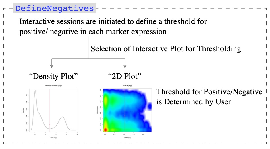
Figure 10: Overview of workflow for DefineNegatives.

User Interaction Workflow:

• Plot Display:

  • The function displays a plot for each marker sequentially.

  • Users can specify a different plot type by setting the y_axis_var argument to another marker name, producing a 2D scatter plot.

  • If ”Density” is chosen for y_axis_var, a density plot (histogram) of the marker’s expression is shown.

• Selecting Threshold Points:

  • Users interactively select points on the plot using the mouse.

  • Each click records a point, and a circle is displayed at the selected location.

  • Users can repeat as many times as needed, adjusting their selection.

  • While setting thresholds, users should consider:

    • For broadly expressed markers like CD45 and CD44, thresholds should distinguish between ’high’ and ’low’ expression levels.

    • For markers with clear separation from background autofluorescence, thresholds should define ’positive’ and ’negative’ populations.

• Finalizing the Threshold:

  • Once satisfied with the x-position (threshold value) of the last selected point, users press the ESC key.

  • The x-coordinate of the last selected point is recorded as the threshold for the current marker.

  • In the GatingTree R package, ’high’ and ’low’ thresholds are treated com- putationally as ’positive’ and ’negative’ to simplify analysis and maintain consistency in the code.

  • The process then moves to the next marker until thresholds for all markers are defined.

2-2. Confirming Thresholds with PlotDefineNegatives:

After setting thresholds with DefineNegatives, use PlotDefineNegatives to visualize and confirm the thresholds:

Visual Confirmation:

x <- PlotDefineNegatives(x, y_axis_var = ’Density’, panel = 4)

This generates plots showing the marker expression distributions with the thresholds indicated by vertical red lines.

Example Outputs:

• Density Plots (Histograms):

  • Visualize the distribution of each marker and the selected threshold.

  • While observing density plots, note the appropriate application of ’high’ vs ’low’ or ’positive’ vs ’negative’ thresholds depending on the marker characteristics.

  • Figure 11 illustrates density plots with thresholds applied.

• 2D Scatter Plots:

  • Specify a marker for the y_axis_var to create scatter plots.

  • Figure 12 shows 2D plots used for threshold confirmation.

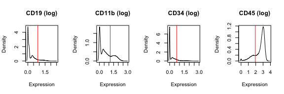
Figure 11: Output of PlotDefineNegatives with the option ’Density’.

The vertical red line indicates the threshold value (Figure 11)..

For 2D plots, choose a variable for the y-axis:

x <- PlotDefineNegatives(x, y_axis_var = "CD3.logdata", panel = 4)

Similarly, the vertical red line indicates the threshold value for x-axis. Note that positions in y-axis are ignored (Figure 12).

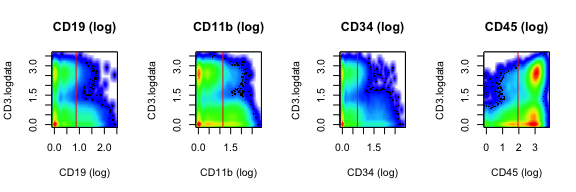
Figure 12: Output of PlotDefineNegatives with the option ’2D-plot’ using CD3 (log) in the y-axis.

2-3. Considerations and Best Practice:

An automated approach using staining controls was tested but found to be impractical. As widely accepted, unstained cells have significantly lower backgrounds than true negative cells in most cases. Extensive use of isotype controls is not practically feasible, and such data cannot be assumed to be consistently available. Furthermore, some markers such as CD45 and CD44 exhibit some degree of staining in the majority of cells analyzed, making the designation of ’high’ and ’low’ possible only through visual inspection of appropriate density plots or 2D plots. Accordingly, manual interactive thresholding remains the recommended method, and future development aims to improve automation in threshold determination. The currently recommended approach emphasizes the necessity of adapting to the specific characteristics of the data, as follows:

• Visual Inspection:

  • Use the density plot option initially to examine the plots for distinct peaks or inflection points.

  • Set thresholds at the points where the expression levels transition between defined states such as ’high’ and ’low’ or ’positive’ and ’negative’. For markers like CD45 and CD44, where a broad expression is observed, thresholds should distinguish between these states based on the actual biological context rather than arbitrary control-derived values. Thus, biological knowledge is crucial for setting appropriate thresholds.

• Adjustments:

  • If the initial thresholds set manually are not satisfactory, it is recommended to rerun DefineNegatives with adjustments based on further visual inspections or additional experimental insights. This iterative approach ensures that the thresholds are optimally set to reflect the true biological variations and experimental conditions.

3. Performing GatingTree Analysis and Visualization

With the data prepared and thresholds defined, perform the GatingTree analysis. Use the createGatingTreeObject function to conduct pathfinding analysis in multidimensional marker space and construct a GatingTree.

x <- createGatingTreeObject(
  x,
  maxDepth = 5,
  min_cell_num = 0,
  expr_group = ’CN’,
  ctrl_group = ’healthy’,
  verbose = FALSE
)

Visualize the GatingTree output:

x <- GatingTreeToDF(x)
node <- x@Gating$GatingTreeObject
datatree <- convertToDataTree(node)
graph <- convert_to_diagrammer(datatree, size_factor = 1, all_labels = FALSE)

library(DiagrammeR)
render_graph(graph, width = 600, height = 600)

This visualizes the entire GatingTree as a tree in a html (Figure 13)

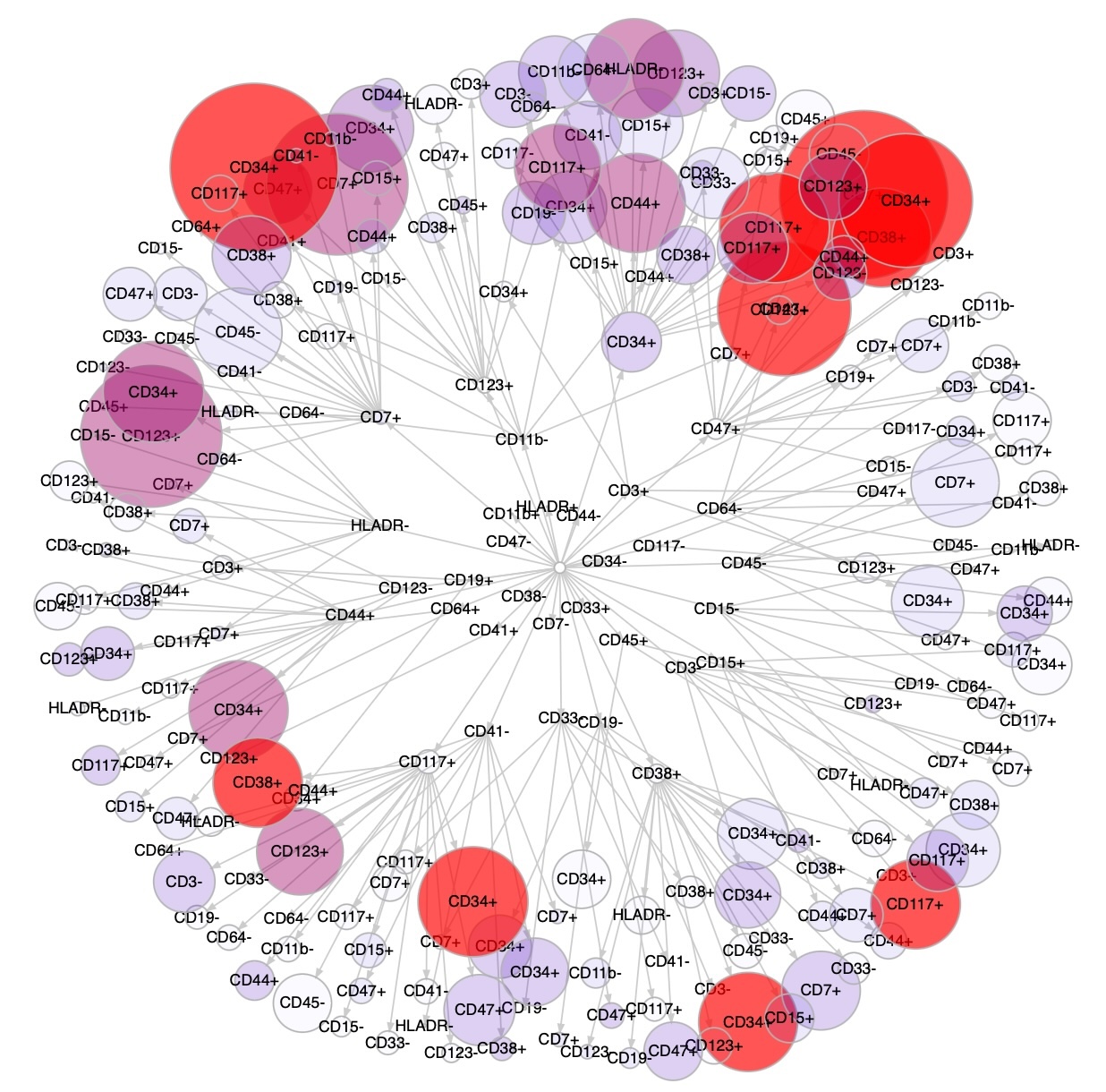
Figure 13: The visualization of the entire GatingTree.

If necessary, prune the GatingTree to focus on the most informative nodes. In the example below, the pruning criteria are set such that the maximum allowable value for gating entropy and the minimum required value for enrichment score are both 0.5:

x <- PruneGatingTree(
  x,
  max_entropy = 0.5,
  min_enrichment = 0.5
)

Visualize the pruned GatingTree:

pruned_node <- x@Gating$PrunedGatingTreeObject
datatree2 <- convertToDataTree(pruned_node)
graph <- convert_to_diagrammer(datatree2, size_factor = 1)
render_graph(graph, width = 600, height = 600)

This visualizes the pruned GatingTree as a tree in a html (Figure 14)

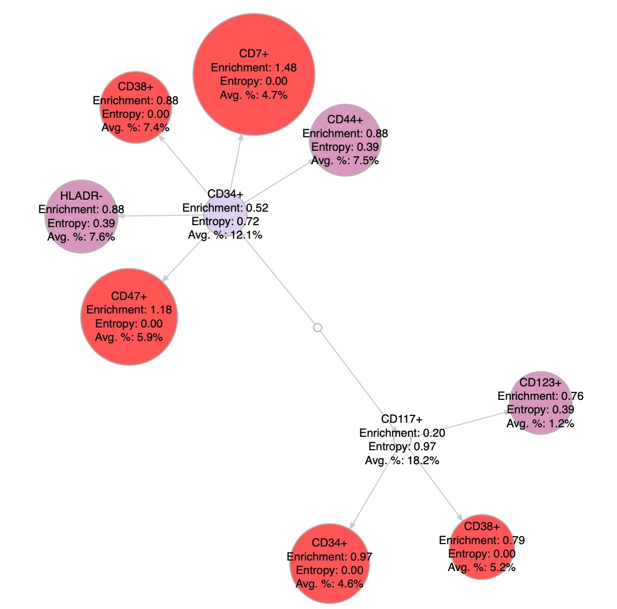
Figure 14: The visualization of the pruned GatingTree.

4. Delta Enrichment Analysis

Finally, assess the impact of adding each marker state to the enrichment score using the PlotDeltaEnrichment function (Figure 15).

x <- PlotDeltaEnrichment(x, significance = FALSE)

Using significance = FALSE, all marker states are shown in Delta Enrichment plot.

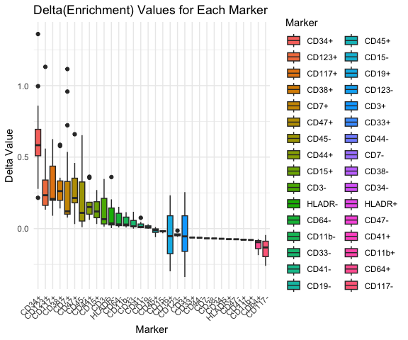
Figure 15: Delta Enrichment Score Analysis.

Discussion

One of the most distinctive features of the proposed Gating Tree method is that its results can be immediately applied by experimentalists as successive gating strategies to identify cell populations of interest. The gates generated by Gating Tree are defined by the set of marker states—whether positive, negative, high, or low. This simplicity in categorizing each marker state is designed to facilitate the planning and execution of repeat or downstream experiments in a robust manner.

As no reliable methods currently exist for automatically setting thresholds for marker positivity, this step is routinely performed manually during data preprocessing. While many experienced immunologists might prefer manual threshold setting, developing methods for automation could be especially beneficial for less experienced users and towards achieving full automation. Thresholds for positivity can be rigorously established by experimentally analyzing staining controls [23]. However, setting thresholds for some markers is necessary to categorize the identification of biologically meaningful cells. For instance, although most CD4⁺ T cells express GITR, only the GITR^high fraction contain cells with unique features such as Foxp3⁺ [24]. Automating this process will require future studies, possibly incorporating community-based data analysis and methods such as transfer learning [25], to establish standardized staining profiles for key antibodies that facilitate data-driven analyses.

Gating Tree analysis, in conjunction with $\Delta E$ analysis, can facilitate the identification of important markers and marker combinations for further investigation. Our studies suggest that analyzing a relatively shallow Gating Tree alongside $\Delta E$ and peak enrichment score analysis provides substantial insights into the data structure and key markers and marker combinations. Future research should aim to develop statistical methods to estimate the coverage of the Turtle’s exploration within the multidimensional marker space and to determine the likelihood of marker combinations for identifying group-specific features.

Future work will concentrate on enhancing the Gating Tree methodology, particularly its application in understanding the data landscape of high-dimensional cytometry. The major limitation of the GatingTree method is that it can be computationally expensive for deep analysis. While the depth of Gating Tree analysis is often limited by the number of available cells rather than computational resources, as shown in Figure 1, deeper analysis may be necessary in certain cases. This will necessitate the development of suitable statistical methods that impose minimal computational burdens. Establishing rigorous statistical methods to evaluate conditional gating probabilities will facilitate the automatic selection of the most promising cell populations. Potential approaches include Bayesian methods, the use of cost functions, and machine learning techniques. The current study has tested the Gating Tree analysis on datasets with up to 24 markers at a depth of 5, experiencing execution times that vary widely—from several seconds to about 24 hours. With the implementation of automatic optimization of conditions, analyzing larger datasets at deeper levels is expected to become more efficient.

We anticipate that the Gating Tree methodology will significantly enhance productivity and refine experimental designs and data acquisition strategies in experimental immunology labs. This advancement is expected to generate robust and useful datasets, further driving the development of this innovative method. Ultimately, this approach will enable more effective and reproducible identification of group-specific features in multidimensional marker datasets for downstream experiments within researchers’ broader research programs, thereby addressing research questions more comprehensively and effectively.

Methods

Definition of Gates

Single Marker Gates: Each marker $m_{k}$ represents a basic gate that defines the logical status (e.g., positive or negative) of each cell for that marker. A single marker gate can be denoted as: $g_{k}=m_{k}$. The probability of a cell passing through a single marker gate $g_{k}$ is given by: $P(g_{k})=P(m_{k})$.

Combined Gates: For sets of markers $\{m_{1},m_{2},\ldots,m_{i}\}$, where each marker determines the logical condition of each cell, we define a combined gate $g_{i}$ using the logical AND operation:

$$g_{i}=m_{1}\land m_{2}\land\ldots\land m_{i}$$

Successive Gates: All gates are defined to be successive and incremental in the Gating Tree method. Thus, if markers are available at the node with the gate $g_{i}$, the next gate $g_{i+1}$ is defined by the addition of another marker, $m_{i+1}$

$$g_{i+1}=m_{1}\land m_{2}\land\ldots\land m_{i}\land m_{i+1}$$

Probability of Successive Gates: Given a parent gate $g_{i}$ with the set $\{m_{1},m_{2},\ldots,m_{i}\}$, the probability is calculated as:

$$P(g_{i})=\prod_{k=1}^{i}P(m_{k}|g_{k-1})$$

where $g_{0}$ is the origin and $p(g_{0})$ is defined to be 1. Hereafter we use log probabilities, i.e.

$$\log(P(g_{i}))=\sum_{k=1}^{i}\log(P(m_{k}|g_{k-1}))$$

Enrichment Score and Differential Enrichment

The enrichment score $E(g_{i})$ is defined as:

$$E(g_{i})=\log\left(\frac{p_{e}(g_{i})}{p_{c}(g_{i})}\right)$$

The differential Enrichment score $\Delta E(g_{i})$ is defined as:

$$\Delta E(g_{i})=E(g_{i})-E(g_{i-1})=\log\left(\frac{p_{e}(g_{i})}{p_{c}(g_{i})}\right)-\log\left(\frac{p_{e}(g_{i-1})}{p_{c}(g_{i-1})}\right)$$

Using the product rule of conditional probability:

$$\Delta E(g_{i})=\log\left(\frac{p_{e}(m_{i}|g_{i-1})\times p_{e}(g_{i-1})\cdot p_{c}(g_{i-1})}{p_{c}(m_{i}|g_{i-1})\times p_{c}(g_{i-1})\cdot p_{e}(g_{i-1})}\right)=\log\left(\frac{p_{e}(m_{i}|g_{i-1})}{p_{c}(m_{i}|g_{i-1})}\right)$$

Thus, the differential Enrichment score between successive gating steps $g_{i}$ and $g_{i-1}$ is given by:

$$\Delta E(g_{i})=\log\left(\frac{p_{e}(m_{i}|g_{i-1})}{p_{c}(m_{i}|g_{i-1})}\right)$$

Note that the calculation of $\Delta E$ employs a base-2 logarithm (log2).

Gating Entropy and Information Gain

Gating entropy is a measure derived from conditional entropy that quantifies the effectiveness of a gating condition in distinguishing between two groups of samples (e.g., Treatment and Control). It assesses how well the gating condition separates the samples based on the percentage of cells meeting certain criteria within each sample.

Overview:

Each sample contains a percentage of cells that meet the gating condition (e.g., being positive for a specific marker). The goal is to determine whether this percentage can effectively distinguish between the two groups of samples. A lower gating entropy indicates a better separation, with an entropy of 0 representing a perfect distinction and an entropy approaching 1 indicating no discriminative power.

Calculation Steps:

1. Compute Group Averages:

For each group (Treatment and Control), calculate the average gated percentage across all samples in that group:

$$\overline{p}_{\text{Treatment}}=\frac{1}{n_{\text{Treatment}}}\sum_{i=1}^{n_{\text{Treatment}}}p_{i}^{\text{Treatment}},\quad\overline{p}_{\text{Control}}=\frac{1}{n_{\text{Control}}}\sum_{i=1}^{n_{\text{Control}}}p_{i}^{\text{Control}},$$

where $p_{i}^{\text{Group}}$ is the gated percentage for sample $i$ in the specified group, and $n_{\text{Group}}$ is the number of samples in that group.

2. Determine the Global Mean Percentage:

Calculate the global mean of the group averages:

$$\mu_{\text{global}}=\frac{n_{\text{Treatment}}\times\overline{p}_{\text{Treatment}}+n_{\text{Control}}\times\overline{p}_{\text{Control}}}{n_{\text{Treatment}}+n_{\text{Control}}}.$$

3. Classify Samples Based on the Global Mean:

For each sample, classify it as ’High’ if its gated percentage exceeds the global mean, or ’Low’ otherwise:

$$\text{Class}_{i}=\begin{cases}\text{'High'}&\text{if }p_{i}>\mu_{\text{global}},\\ \text{'Low'}&\text{if }p_{i}\leq\mu_{\text{global}}.\end{cases}$$

4. Construct the Contingency Table:

Create a contingency table that cross-tabulates the sample classifications (’High’ or ’Low’) against the actual group labels (Treatment or Control):

	Treatment	Control
High	$n_{\text{High,Treatment}}$	$n_{\text{High,Control}}$
Low	$n_{\text{Low,Treatment}}$	$n_{\text{Low,Control}}$

5. Calculate Conditional Probabilities:

For each classification (’High’ or ’Low’), compute the probabilities of being in each group:

$$p(\text{Group}|\text{Class})=\frac{n_{\text{Class,Group}}}{n_{\text{Class}}},$$

where $n_{\text{Class}}$ is the total number of samples classified as ’High’ or ’Low’.

6. Compute the Gating Entropy:

The gating entropy $H(\text{Group}|\text{Class})$ is calculated using the conditional entropy formula:

$$H(\text{Group}|\text{Class})=-\sum_{\text{Class}\in\{\text{High},\text{Low}\}}p(\text{Class})\sum_{\text{Group}\in\{\text{Treatment},\text{Control}\}}p(\text{Group}|\text{Class})\log_{2}p(\text{Group}|\text{Class}),$$

where $p(\text{Class})=\frac{n_{\text{Class}}}{n_{\text{Total}}}$ is the proportion of samples in each classification.

7. Baseline Entropy at the root node $H(Y)$, without any gating condition, is defined as follows:

$$H(Y)=-\sum_{k\in\{\text{Treatment},\text{Control}\}}p(k)\log_{2}p(k)$$

Interpretation:

- An entropy of 0 indicates perfect discrimination, where each classification (’High’ or ’Low’) contains samples from only one group. - An entropy close to 1 suggests that the gating condition does not distinguish between the groups, with the classifications containing an even mix of Treatment and Control samples.

Example:

Suppose we have the following data:

- Treatment group: 3 samples with gated percentages of 80%, 85%, and 90%. - Control group: 3 samples with gated percentages of 10%, 15%, and 20%.

Calculation:

1. Compute group averages:

$$\overline{p}_{\text{Treatment}}=\frac{80+85+90}{3}=85\%,\quad\overline{p}_{\text{Control}}=\frac{10+15+20}{3}=15\%.$$

2. Determine the global mean:

$$\mu_{\text{global}}=\frac{3\times 85\%+3\times 15\%}{6}=50\%.$$

3. Classify samples:

- Samples with percentages above 50% are classified as ’High’. - Treatment samples: all ’High’. - Control samples: all ’Low’.

4. Contingency table:

	Treatment	Control
High	3	0
Low	0	3

5. Calculate probabilities:

- $p(\text{High})=\frac{3}{6}=0.5$, $p(\text{Treatment}|\text{High})=1$, $p(\text{Control}|\text{High})=0$. - $p(\text{Low})=\frac{3}{6}=0.5$, $p(\text{Treatment}|\text{Low})=0$, $p(\text{Control}|\text{Low})=1$.

6. Compute gating entropy:

$$H(\text{Group}|\text{Class})=-[0.5\times(1\times\log_{2}1+0\times\log_{2}0)+0.5\times(0\times\log_{2}0+1\times\log_{2}1)]=0.$$

This result indicates perfect discrimination between the Treatment and Control groups using the gating condition.

Pruning of Gating Tree

To prune the Gating Tree, the Gating Tree object is traversed to collect the enrichment score, entropy, and the average percentage of cells relative to the total cells for all nodes, resulting in a data frame. Thresholds are then established to filter out nodes with low enrichment scores, high entropy, or an insufficient number of cells. Nodes in the Gating Tree are subsequently labeled as either to be pruned (Prune = TRUE) or retained (Prune = FALSE). This labeling facilitates the systematic pruning of the Gating Tree.

After pruning the Gating Tree, statistical tests may be employed to validate the remaining nodes. Given that percentage data are better tested using a non-parametric test, the current implementation utilizes the Mann-Whitney test with p-value adjustments for the false discovery rate to ensure robust statistical conclusions.

Datasets and Performance Testing

The AML-sim and PD-1 datasets were from the R package HDCytoData [22]. A mixed Gaussian data was generated by sampling autofluorescence cells from $\mathcal{N}(1000,100^{2})$ and marker positive cells from $\mathcal{N}(2000,200^{2})$ for nine markers independently and randomly. The final dataset $\mathbf{D}$ is obtained by applying logarithmic transformation. Subsequently, the proportion of target cell cluster, m8+ m9+ m10+ cells within each data was identified, randomly reassigned within the dataset to simulate additional cell factor influences (injected cells).

Performance testing was conducted using the R packages pROC [26] and PRROC [27]. Self-Origanizing Map (FlowSOM) was used for identifying clusters as a control method [1].

Implementation

The Gating Tree method is implemented as an R package using base R functions. Tree visualization is realised by importing functions from the CRAN packages DiagrammeR[28] and data.tree [29].

Code availability

The source code for the GatingTree software, implemented as an R package, is freely available through the MonoTockyLab GitHub repository (https://github.com/MonoTockyLab/GatingTree).

References

Supplementary information

References

- [1] Sofie Van Gassen, Britt Callebaut, Mary J. Van Helden, Bart N. Lambrecht, Piet Demeester, Tom Dhaene, and Yvan Saeys. Flowsom: Using self-organizing maps for visualization and interpretation of cytometry data. Cytometry Part A, 87(7):636–645, 2015.
- [2] Hiroko Fujii, Julie Josse, Miki Tanioka, Yoshiki Miyachi, François Husson, and Masahiro Ono. Regulatory t cells in melanoma revisited by a computational clustering of foxp3+ t cell subpopulations. The Journal of Immunology, 196(6):2885–2892, 2016.
- [3] Kenneth Lo, Florian Hahne, Ryan R. Brinkman, and Raphael Gottardo. flowclust: a bioconductor package for automated gating of flow cytometry data. BMC Bioinformatics, 10(1):145, 2009.
- [4] Eirini Arvaniti and Manfred Claassen. Sensitive detection of rare disease-associated cell subsets via representation learning. Nature Communications, 8(1):14825, 2017.
- [5] A. Cossarizza, H. D. Chang, A. Radbruch, S. Abrignani, R. Addo, M. Akdis, I. Andrä, F. Andreata, et al. Guidelines for the use of flow cytometry and cell sorting in immunological studies (third edition). Eur J Immunol, 51(12):2708–3145, 2021.
- [6] Masahiro Ono, Reiko Tanaka, and Manabu Kano. Visualisation of the t cell differentiation programme by canonical correspondence analysis of transcriptomes. BMC Genomics, 15, 2014. This study establishes CCA as a vital quantitative tool for transcriptome analysis in immunological datasets.
- [7] Tara Chari and Lior Pachter. The specious art of single-cell genomics. PLOS Computational Biology, 19(8):1–20, 08 2023.
- [8] Lukas M. Weber, Malgorzata Nowicka, Charlotte Soneson, and Mark D. Robinson. diffcyt: Differential discovery in high-dimensional cytometry via high-resolution clustering. Communications Biology, 2(1):183, 2019.
- [9] Etienne Becht, Yannick Simoni, Elaine Coustan-Smith, Maximilien Evrard, Yang Cheng, Lai Guan Ng, Dario Campana, and Evan W Newell. Reverse-engineering flow-cytometry gating strategies for phenotypic labelling and high-performance cell sorting. Bioinformatics, 35(2):301–308, 06 2018.
- [10] Stefano Mangiola, Alexandra J. Roth-Schulze, Marie Trussart, Enrique Zozaya-Valdés, Mengyao Ma, Zijie Gao, Alan F. Rubin, Terence P. Speed, Heejung Shim, and Anthony T. Papenfuss. sccomp: Robust differential composition and variability analysis for single-cell data. Proceedings of the National Academy of Sciences, 120(33):e2203828120, 2023.
- [11] D. Okada, J. H. Cheng, C. Zheng, and R. Yamada. Data-driven comparison of multiple high-dimensional single-cell expression profiles. J Hum Genet, 67(4):215–221, 2022.
- [12] Masahiro Ono, Reiko Tanaka, Manabu Kano, and Toshio Sugiman. Visualising the cross-level relationships between pathological and physiological processes and gene expression: analyses of haematological diseases. PLoS One, 8(1):e53544, 2013. The pioneering study developing Canonical Correspondence Analysis (CCA) as a genomics method, establishing a novel approach for transcriptome analysis.
- [13] Alla Bradley, Tetsuo Hashimoto, and Masahiro Ono. Elucidating t cell activation-dependent mechanisms for bifurcation of regulatory and effector t cell differentiation by multidimensional and single-cell analysis. Frontiers in Immunology, 9, 2018.
- [14] Sjoerd T T Schetters, Ernesto Rodriguez, Laura J W Kruijssen, Matheus H W Crommentuijn, Louis Boon, Jan Van den Bossche, Joke M M Den Haan, and Yvette Van Kooyk. Monocyte-derived apcs are central to the response of pd1 checkpoint blockade and provide a therapeutic target for combination therapy. Journal for ImmunoTherapy of Cancer, 8(2), 2020.
- [15] X. Shi, G. V. Baracho, 3rd Lomas, W. E., S. J. Widmann, and A. J. Tyznik. Co-staining human pbmcs with fluorescent antibodies and antibody-oligonucleotide conjugates for cell sorting prior to single-cell cite-seq. STAR Protoc, 2(4):100893, 2021.
- [16] T. Takeuchi and H. Ohno. Analysis of peripherally derived treg in the intestine. Methods Mol Biol, 2559:41–49, 2023.
- [17] V. da Silva Domingues, I. Caramalho, M. L. Bergman, and J. Demengeot. Adoptive transfer and bone marrow chimera models to analyze treg function and differentiation. Methods Mol Biol, 2559:15–29, 2023.
- [18] H. Barcenilla, M. Pihl, F. Sjögren, L. Magnusson, and R. Casas. Regulatory t-cell phenotyping using cytof. Methods Mol Biol, 2559:231–242, 2023.
- [19] Anna C. Belkina, Caroline E. Roe, Vera A. Tang, Jessica B. Back, Claudia Bispo, Alexis Conway, Uttara Chakraborty, Kathleen T. Daniels, Gelo de la Cruz, Laura Ferrer-Font, Andrew Filby, David M. Gravano, Michael D. Gregory, Christopher Hall, Christian Kukat, André Mozes, Diana Ordoñez-Rueda, Eva Orlowski-Oliver, Isabella Pesce, Ziv Porat, Nicole J. Poulton, Kristen M. Reifel, Aja M. Rieger, Rachael T. C. Sheridan, Gert Van Isterdael, and Rachael V. Walker. Guidelines for establishing a cytometry laboratory. Cytometry Part A, 105(2):88–111, 2024.
- [20] C. Krieg, M. Nowicka, S. Guglietta, S. Schindler, F. J. Hartmann, L. M. Weber, R. Dummer, M. D. Robinson, M. P. Levesque, and B. Becher. High-dimensional single-cell analysis predicts response to anti-pd-1 immunotherapy. Nat Med, 24(2):144–153, 2018.
- [21] Jehanne Hassan, Elizabeth Appleton, Bahire Kalfaoglu, Malin Pedersen, José Almeida-Santos, Hisashi Kanemaru, Nobuko Irie, Shane Foo, Omnia Reda, Benjy J.Y. Tan, Il-mi Okazaki, Taku Okazaki, Yorifumi Satou, Kevin Harrington, Alan Melcher, and Masahiro Ono. Single-cell level temporal profiling of tumour-reactive t cells under immune checkpoint blockade. bioRxiv, page 2022.07.19.500582, 2022.
- [22] L. M. Weber and C. Soneson. Hdcytodata: Collection of high-dimensional cytometry benchmark datasets in bioconductor object formats. F1000Res, 8:1459, 2019.
- [23] Ruud Hulspas, Maurice R.G. O’Gorman, Brent L. Wood, Jan W. Gratama, and D. Robert Sutherland. Considerations for the control of background fluorescence in clinical flow cytometry. Cytometry Part B: Clinical Cytometry, 76B(6):355–364, 2009.
- [24] Masahiro Ono, Jun Shimizu, Yoshiki Miyachi, and Shimon Sakaguchi. Control of autoimmune myocarditis and multiorgan inflammation by gitr high, foxp3-expressing cd25 positive and cd25 negative regulatory t cells. The Journal of Immunology, 176(8):4748–4756, 2006.
- [25] Philip Ganchev, David Malehorn, William L. Bigbee, and Vanathi Gopalakrishnan. Transfer learning of classification rules for biomarker discovery and verification from molecular profiling studies. Journal of Biomedical Informatics, 44:S17–S23, 2011. Supplement: AMIA Joint Summits on Translational Science – 2011.
- [26] Xavier Robin, Natacha Turck, Alexandre Hainard, Natalia Tiberti, Frédérique Lisacek, Jean-Charles Sanchez, and Markus Müller. proc: an open-source package for r and s+ to analyze and compare roc curves. BMC Bioinformatics, 12:77, 2011.
- [27] Jens Keilwagen, Ivo Grosse, and Jan Grau. Area under precision-recall curves for weighted and unweighted data. PLOS ONE, 9(3), 2014.
- [28] Richard Iannone and Olivier Roy. DiagrammeR: Graph/Network Visualization, 2024. R package version 1.0.11.
- [29] Christoph Glur. data.tree: General Purpose Hierarchical Data Structure, 2023. R package version 1.1.0.