Soft Condorcet Optimization for Ranking of General Agents

Abstract

A common way to drive progress of AI models and agents is to compare their performance on standardized benchmarks. Comparing the performance of general agents requires aggregating their individual performances across a potentially wide variety of different tasks. In this paper, we describe a novel ranking scheme inspired by social choice frameworks, called Soft Condorcet Optimization (SCO), to compute the optimal ranking of agents: the one that makes the fewest mistakes in predicting the agent comparisons in the evaluation data. This optimal ranking is the maximum likelihood estimate when evaluation data (which we view as votes) are interpreted as noisy samples from a ground truth ranking, a solution to Condorcet’s original voting system criteria. SCO ratings are maximal for Condorcet winners when they exist, which we show is not necessarily true for the classical rating system Elo. We propose three optimization algorithms to compute SCO ratings and evaluate their empirical performance. When serving as an approximation to the Kemeny-Young voting method, SCO rankings are on average 0 to 0.043 away from the optimal ranking in normalized Kendall-tau distance across 865 preference profiles from the PrefLib open ranking archive. In a simulated noisy tournament setting, SCO achieves accurate approximations to the ground truth ranking and the best among several baselines when 59% or more of the preference data is missing. Finally, SCO ranking provides the best approximation to the optimal ranking, measured on held-out test sets, in a problem containing 52,958 human players across 31,049 games of the classic seven-player game of Diplomacy.

1 Introduction

Progress in the field of artificial intelligence has been driven by measuring the performance of agents on common benchmarks and challenge problems. AI pioneers designed checkers-playing agents (Samuel, 1959), then strove for super-human performance chess (Campbell et al., 2002), and then in other games such as Backgammon (Tesauro, 1995), Arimaa (Syed, ), Go (Silver et al., 2016), Starcraft (Vinyals et al., 2019) and Diplomacy († et al.(2022)(FAIR)†, Bakhtin, Brown, Dinan, Farina, Flaherty, Fried, Goff, Gray, Hu, Jacob, Komeili, Konath, Kwon, Lerer, Lewis, Miller, Mitts, Renduchintala, Roller, Rowe, Shi, Spisak, Wei, Wu, Zhang, and Zijlstra, FAIR). In machine learning, common benchmarks like the UCI data set repository allowed direct comparisons of supervised learning algorithms (Kelly et al., ). Competitions, such as ImageNet, led to breakthroughs in deep learning (Krizhevsky et al., 2012).

All of these examples require comparing agents (or models). Original success stories such as DeepBlue, TD-Gammon, and AlphaGo focused on a single domain. In the past ten years, agents have become increasingly more generally capable. AlphaZero extended application of AlphaGo to chess and Shogi (Silver et al., 2018). The Arcade Learning Environment (Bellemare et al., 2013), which steered much of the agent development in deep reinforcement learning, evaluated agents across 57 different Atari games. Recently, language models have been evaluated across suites of tasks such as in HELM (Liang et al., 2022), BIG-bench (bench authors, 2023) AgentBench (Liu et al., 2023), and via a public leaderboard such as Chatbot Arena driven by human voting (Chiang et al., 2024). Answering simple questions for these generally capable agents, such as “Which is the best agent?” or “Is agent $X$ better than agent $Y$?” or “What is the relative ranking of agents $X$, $Y$, and $Z$?” become increasingly more difficult when aggregating over many different contexts: how agents are scored may vary wildly across tasks, data collected for evaluation may not be balanced evenly across tasks (or agents), and classical rating systems were simply not designed for this use case.

To address these problems, recent ranking methods such as Vote’N’Rank (Rofin et al., 2023) and Voting-as-Evaluation (VasE) (Lanctot et al., 2023) use voting methods to aggregate results across tasks. Using computational social choice as a basis for ranking agents has several benefits: these systems have been well-studied and understood for a long time, they inherit consistency properties of the voting methods they are based on, they do no require score normalization, and are less sensitive to score values and agent population than game-theoretic evaluation schemes such as Nash averaging (Balduzzi et al., 2018). However, classic voting schemes, and related tournament solutions, typically assume that the data (e.g. agent comparisons) is complete. This assumption is not necessarily valid in the agent evaluation setting. For example, on the webDiplomacy web site (webDiplomacy Development Team, ) there were 52,958 unique (human) agents across only 31,049 seven-player games played between 2008 and 2019: most players have not played against most other players; hence, there are no direct comparisons between the vast majority ($\geq 99\%$) of agent pairs. While there has been research on identifying “necessary and possible winners” when there is incomplete voting or comparison data, the results are mixed (Pini et al., 2011; Xia and Conitzer, 2011; Aziz et al., 2015) and most of the findings are focused on identifying top-ranked agents, not ranking all agents as is our focus.

In this paper, we introduce a new ranking scheme for general agents inspired by the interpretation of voting rules as maximum likelihood estimators (Conitzer and Sandholm, 2005). Starting with Condorcet’s original model of voting (Brandt et al., 2016, Chapter 8), Young showed that the maximum likelihood estimate (MLE) of the true ranking is the one that minimizes the sum of Kendall-tau distances to all the votes. This also corresponds to the ranking found by Kemeny’s voting rule (Kemeny, 1959). Finding this solution directly is computationally expensive and does not scale to many agents, a regime that is common in the agent evaluation setting. Like classical rating systems for agent evaluation (such as Elo (Elo, 1978) and TrueSkill (Herbrich et al., 2006)), Soft Condorcet Optimization (SCO) assigns a numerical rating (score) $\theta_{a}$ to each agent (alternative) $a$. SCO then treats these ratings as a parameter vector, the votes as a data set, and defines a differentiable loss function as the objective. The final ranking of agents is obtained by sorting the ratings.

In summary, this paper makes the following contributions:

• The SCO ranking scheme with the following properties:

  • Three optimization methods to find ratings and corresponding rankings: gradient descent applied to (i) a soft Kendall-tau distance (“sigmoid loss”), or (ii) a Fenchel-Young loss (perturbed optimization) (Berthet et al., 2020); or (iii) solving a sigmoidal program with a branch-and-bound method (Udell and Boyd, 2014).

  • Online forms that can update ratings, and thus rankings, from individual outcomes as evaluation data arrives.

  • Theorem 1, guaranteeing that the top-ranked agent by SCO ratings according to the sigmoid loss is the Condorcet winner when one exists.

• Empirical evaluations that demonstrate the following:

  • SCO ranking using sigmoid loss solves a failure mode of classical Elo rating system which may top-rank an agent that is not a Condorcet winner even when one exists.

  • SCO can serve as an approximation to the Kemeny-Young voting method, indeed empirically finding low approximation error to the optimal ranking: on average 0 to 0.043 away in normalized Kendall-tau distance across 865 preference profiles from the PrefLib (Mattei and Walsh, 2013) repository.

  • In a noisy tournament setting with sparse data, SCO approximates the true ranking best when a large proportion (59% or more) of the data is missing.

  • SCO ratings are closer to optimal rankings than Elo and voting-as-evaluation methods on held out test sets over 31,049 human Diplomacy games played by 52,958 players.

2 Background

In this section, we describe the building blocks and introduce some basic terminology required to understand our method.

2.1 Evaluation of General Agents

We first paraphrase several key descriptions from (Balduzzi et al., 2018; Lanctot et al., 2023). The problem of evaluating agents is that of ranking agents according to their skill. Skill can be determined in several ways. In the Agent-versus-Task (AvT) setting, agents compete individually in different tasks and compare outcomes (scores) to each other in each task (e.g., language models and the various metrics for assessing their abilities). In the Agent-versus-Agent (AvA) setting, agents directly compete against each other (e.g., online games such as chess or Diplomacy).

2.1.1 Classical Evaluation

Elo is a classic rating system that uses a simple logistic model learned from win/loss/draw outcomes (Elo, 1978). A rating, $r_{i}$, is assigned to each player $i$ such that the probability of player $i$ beating player $j$ is predicted as $\hat{p}_{ij}=\frac{1}{1+10^{(r_{j}-r_{i})/400}}$. While Elo was designed specifically to rate players in the two-player zero-sum, perfect information game of Chess, it has been widely applied to other domains, including in evaluation of large language models (Zheng et al., 2023). TrueSkill (Herbrich et al., 2006) and bayeselo (Coulom, 2005) are rating systems based on similar foundations (Bradley-Terry models of skill) that also model uncertainty over ratings using Bayesian methods.

Elo has a number of positive qualities. First, it is a simple rule. Second, it can be used to estimate win rates between any two agents. Third, it can be easily employed online, i.e., to modify players’ ratings from the result of a single game. It is also a special case of logistic regression (for details, see Appendix C.2). Hence, Elo has been widely applied and is a common default choice for evaluation of agents. However, Elo has a number of well-known drawbacks (Balduzzi et al., 2018; Lanctot et al., 2023; Bertrand et al., 2023). Of particular interest is the incompatibility of Elo with the concept of a Condorcet winner from social choice theory; examples are summarized in Section 4.1.

2.1.2 Voting as Evaluation of General Agents

Another way to evaluate agents is to use social choice theory, called Voting-as-Evaluation (VasE) recently proposed in (Lanctot et al., 2023). In VasE, the alternatives correspond to general agents and votes to assessments of their performance. In the AvT setting, agents are ordered based on their performance on different tasks (such as each game in the Atari Learning Environment (Bellemare et al., 2013) or on different benchmarks for large language models (Liu et al., 2023)). In the AvA setting, agents compete directly in a multiagent environment, such as multiplayer games (like chess or poker), and each game outcome corresponds to a ranking over a subset of agents. Chatbot Arena (Zheng et al., 2023), where language models compete head-to-head to provide the best answer to the same question, is another instance of the AvA setting. Casting agent evaluation as an application of computational social choice provides the benefit of robustness in the form of Condorcet consistency, clone/composition consistency, agenda consistency, and/or population consistency depending on the choice of voting rule used to evaluate agents. However, it is unclear how well these methods perform when the data is missing or unevenly distributed, which often occurs in the agent evaluation setting. SCO is motivated similarly to VasE and, as such, will be empirically assessed mainly for agent evaluation. To make the connection to ideas from the social choice literature, we will often use voting language when discussing SCO and its use in evaluation. Relevant terminology is introduced later in the paper.

2.2 Permutation and Ranking Distances

We now define distance metrics over rankings that will play a key role when describing our method and loss function. Informally, the Kendall-tau distance counts the number of pairwise disagreements between permutations.

Definition 1.

Let $S_{1},S_{2}$ be finite sets of elements such that $S_{1}\subseteq S_{2}$. Let $\pi_{1},\pi_{2}$ be permutations over elements in $S_{1}$ and $S_{2}$, respectively. The Kendall-tau distance between two permutations is defined as

$$K_{d}(\pi_{1},\pi_{2})=\sum_{\{i,j\}\in\mathcal{C}_{2}(S_{1})}\bar{K}_{i,j}(\pi_{1},\pi_{2}),$$ (1)

where $\mathcal{C}_{2}(S)$ is the set of unordered pairs of $S$ (combinations of size 2), $\bar{K}_{i,j}(\pi_{1},\pi_{2})=0$ if $i$ and $j$ are in the same order in $\pi_{1}$ and $\pi_{2}$, and $\bar{K}_{i,j}(\pi_{1},\pi_{2})=1$ otherwise.

Note that this definition allows one set to be a subset of the other, which is more general than the standard definition; this distinction is necessary for the evaluation metric used in Section 4.4, and corresponds to the standard definition when $S_{1}=S_{2}$.

Since the maximum distance is ${|S_{1}|\choose 2}=\frac{|S_{1}|(|S_{1}|-1)}{2}$, this can be easily normalized to be in $[0,1]$:

Definition 2.

Let $S_{1},S_{2}$ be finite sets of elements such that $S_{1}\subseteq S_{2}$. Let $\pi_{1},\pi_{2}$ be permutations over elements in $S_{1}$ and $S_{2}$, respectively. The normalized Kendall-tau distance $\pi_{1}$ and $\pi_{2}$ is defined as

$$K_{n}(\pi_{1},\pi_{2})=\frac{2K_{d}(\pi_{1},\pi_{2})}{|S_{1}|(|S_{1}|-1)}.$$ (2)

2.3 Social Choice Theory

A voting scheme is defined as $\langle A,V,f\rangle$ where $A=\{a_{1},\ldots,a_{m}\}$ is the set of alternatives (agents), $V=\{v_{1},\ldots,v_{n}\}$ is the set of voters, and $f$ is the voting rule that determines how votes are aggregated. Voters have preferences over alternatives: $a_{1}\succ_{v_{i}}a_{2}$ indicates voter $v_{i}$ strictly prefers alternative $a_{1}$ over alternative $a_{2}$, and $a_{1}\succeq_{v_{i}}a_{2}$ indicates the voter has a weak preference. These preferences induce (nonstrict) total orders over alternatives, which we denote by $\mathcal{L}$. A preference profile, $[\succeq]\in\mathcal{L}^{n}$, is a vector specifying the preferences of each voter in $V$. It can be useful to summarize the preference profile in a voter preference matrix $\mathbf{N}$ or vote margin matrix $\mathbf{M}$. The preference count $N(x,y)$, $x,y\in A$ is the number of voters in $[\succeq]$ that strictly prefer $x$ to $y$. The vote margin is the difference in preference count: $\delta(x,y)=N(x,y)-N(y,x)$. Table 1 shows a preference profile and its resulting preference matrix, $\mathbf{N}=(N(i,j))_{i,j}$, and margin matrix $\mathbf{M}=(\delta(i,j))_{i,j}=\mathbf{N}-\mathbf{N}^{T}$.

The central problem of social choice theory is how to aggregate preferences of a population so as to reach some collective decision. A voting rule that determines the “winner” (a non-empty subset, possibly with ties), is a social choice function (SCF). A voting rule that returns an aggregate ranking (total order) over all the alternatives is a social welfare function (SWF). Much of the social choice literature focuses on understanding what properties different voting rules support.

The Condorcet winner defines a fairly intuitive concept: $A$ is the (strong) Condorcet winner if the number of votes where $A$ is ranked higher than $B$ is greater than vice versa for all other alternatives $B$. A weak Condorcet winner wins or ties in every head-to-head pairing. Formally, given a preference profile, $[\succeq]$, a weak Condorcet winner is an alternative $a^{*}\in A$ such that $\forall a^{\prime}\in A,\delta(a^{*},a^{\prime})\geq 0$. If the inequality is strict for all pairs except $(a^{*},a^{*})$ then we call it a strong Condorcet winner. In the example shown in Table 1, alternative $C$ is the strong Condorcet winner. It dominates $A$ since three out of the five voters prefer $C$ to $A$. A similar situation holds when $C$ is compared to alternative $B$. While many have argued that this definition captures the essence of the correct collective choice (de Condorcet, 1785), in practice preference profiles may have no Condorcet winner. Condorcet-consistent voting schemes (e.g., Kemeny-Young introduced next) return a Condorcet winner when it exists, but differ on how they handle settings with no Condorcet winners.

1:	$A\succ B\succ C$
1:	$A\succ C\succ B$
2:	$C\succ A\succ B$
1:	$B\succ C\succ A$

	$A$	$B$	$C$
$A$	0	4	2
$B$	1	0	2
$C$	3	3	0

	$A$	$B$	$C$
$A$	0	3	-1
$B$	-3	0	-1
$C$	1	1	0

Table 1: Left: an example preference profile with five votes (Lanctot et al., 2023, Figure 1). The number on the left of the colon represents the number of votes of that type. Middle: the voter preference matrix, $\mathbf{N}$. Right: the voter margin matrix, $\mathbf{M}$.

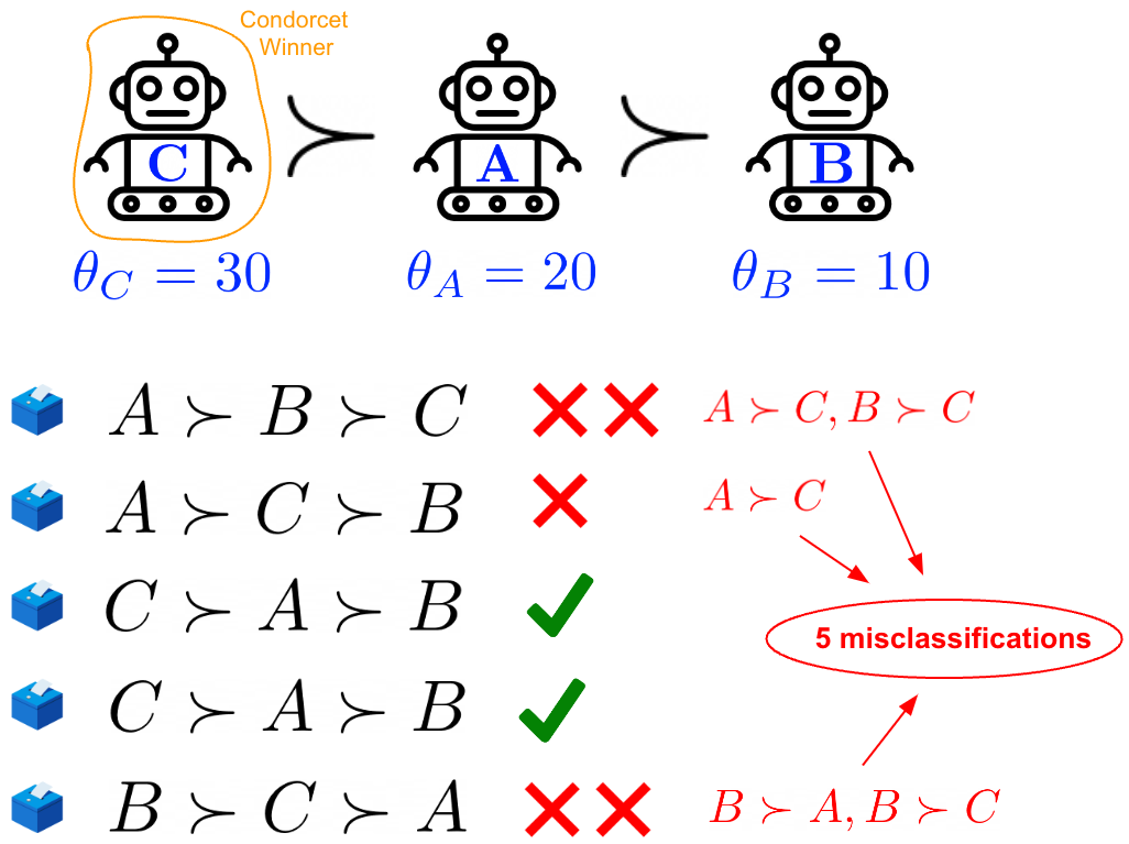
Figure 1: An example calculation of the Kendall-tau distances of each vote in the preference profile from Table 1 to the optimal ranking $R=C\succ A\succ B$. The sum of the distances is 5. This sum for any other ranking $R^{\prime}\not=R$ is greater than 5.

2.3.1 Kemeny-Young Voting Method

The voting method was initially proposed by Kemeny (Kemeny, 1959). Later, its properties were characterized by Young & Levenglick  (Young and Levenglick, 1978). Let each ranking (total order) be represented as a permutation $\pi$ over $|A|$ alternatives. Define the Kemeny score of permutation $\pi$ as

$$\textsc{KemenyScore}(\pi)=\sum_{(i,j),i<j}N(\pi[i],\pi[j]).$$

The Kemeny rule returns a ranking that maximizes this: $\operatornamewithlimits{argmax}_{\pi\in\Pi(|A|)}\textsc{KemenyScore}(\pi)$. Kemeny-Young is Condorcet-consistent: if a Condorcet winner exists, it will be top-ranked by Kemeny-Young. It also satisfies the majority criterion, the Smith criterion (Smith, 1973), and monotonicity. The Kemeny rule always returns an optimal ranking, i.e., one whose sum of Kendall-tau distances to the votes is minimal, but its computational complexity is prohibitively expensive when $m$ is large.

2.4 Learning-to-Rank

Another related field is that of learning-to-rank (Liu, 2011). The canonical example is that of a search engine: a user enters a keyword (query) and the problem is to retrieve the most relevant documents in a database, ranked by relevance to the keyword. There are several algorithms that learn to rank; Google’s PageRank, which powers their search engine, is one example. Our setting can be characterized by a learning-to-rank problem with a constant keyword (or no keyword) as there is no query. An important class of statistical models in this setting is random utility models (Xia, 2019). In random utility models, assessments are perceived as some ground truth assessment plus some noise.

Perturbed optimizers (Berthet et al., 2020; Blondel et al., 2020b) transform non-differentiable functions (such as sorting and ranking) into smoothed versions by adding noise; these perturbed functions can then be optimized by gradient descent. This is part of a growing effort to allow end-to-end training through discrete operators, using classical stochastic smoothing and perturbation approaches (Gumbel, 1954; Hazan et al., 2016). Included are optimal transport, clustering, dynamic time-warping and other dynamic programs (Cuturi, 2013; Cuturi and Blondel, 2017; Mensch and Blondel, 2018; Vlastelica et al., 2019; Paulus et al., 2020; Sander et al., 2023; Stewart et al., 2022) applied in fields such as computer vision, audio processing, biology, and physical simulators (Cordonnier et al., 2021; Kumar et al., 2021; Carr et al., 2021; Le Lidec et al., 2021; Baid et al., 2023; Llinares-López et al., 2023) and other optimization algorithms (Dubois-Taine et al., 2022).

3 Soft Condorcet Optimization

Soft Condorcet Optimization (SCO) is a ranking scheme for evaluation of general agents inspired by social choice theory. An SCO ranking is derived from and represented by SCO ratings, $\theta_{a}$, for each alternative $a\in A$. The rating $\theta_{a}\in[\theta_{\min},\theta_{\max}]$ serves only to determine $a$’s relative order compared to other alternatives in the ranking, such that $a\succ b$ if and only if $\theta_{a}>\theta_{b}$. The ranking is induced by numerically sorting these ratings (e.g., see Figure 1). We then formulate an optimization problem by carefully constructing a loss function that that penalizes discrepancies or misclassifications in the ordinal relationships between alternatives.

An SCO rating is a numerical value representing an agent’s level of skill compared to other agents. SCO is closely related to several prior works: Elo (Elo, 1978), probabilistic ranking (Diaconis, 1988; Marden, 1995; Alvo and Yu, 2014), and perturbed optimizers (Blondel et al., 2020b; Berthet et al., 2020). We elaborate on these relationships in Appendix C. We now present the main ideas followed by different ways to compute the SCO ratings.

3.1 SCO Ratings and the Sigmoid Loss

In this section, we first explain the sigmoid loss function. For some set of ratings $\bm{\theta}$, this loss function quantifies the amount of error: the level of disagreement between the specific values of each rating and the data (preference profiles obtained through agent evaluation). The goal is then to find an assignment of ratings that minimizes this loss, i.e., the set of ratings that best explain the preference data.

Let $\Pi(A)$ denote the set of permutations over alternatives $A$. We will call the data we work with “votes” to emphasize that we are working with (partial) rankings over alternatives, and borrow terminology from preferences and social choice. In particular, we view the entire dataset to be a collection of votes and so will refer to it as preference profile, $[\succeq]$. Let $v\in[\succeq]$ refer to each vote in the profile, where $v$ is a permutation over subsets of $A$, with length $|v|$. For a vote $v$, denote $v[i]$ as the alternative in position $i$ such that vote $v$ is represented as: $v[0]\succ v[1]\succ\cdots\succ v[|v|-1]$.

The ultimate goal is to find an optimal ranking $R$:

Definition 3.

Given some a profile $[\succeq]$ (i.e., set of votes), an optimal ranking minimizes the sum of the Kendall-tau distances

$$R=argmin_{R\in\Pi(A)}\sum_{v\in[\succeq]}K_{d}(v,R).$$

Let index pairs $I_{2}(v)=\{(i,j)\leavevmode\nobreak\ |\leavevmode\nobreak\ i,j\in\{0,1,\cdots,|v|-1\}\mbox{ and }i<j\}$. Given a preference profile and ratings $\bm{\theta}$, we define a discrete loss:

$$L([\succeq],A,V,\bm{\theta})=\sum_{v\in[\succeq]}\sum_{(i,j)\in I_{2}(v)}D_{v}(\theta_{v[i]},\theta_{v[j]}),$$ (3)

where $D_{v}(\theta_{a},\theta_{b})$ is a function that measures the discrepancy between the positions of alternatives $a$ and $b$:

$$D_{v}(\theta_{a},\theta_{b})=\left\{\begin{array}[]{ll}1&\mbox{if $\theta_{b}-\theta_{a}>0$ in $v$};\\ 0&\mbox{otherwise},\end{array}\right.,$$ (4)

then the minimum of the discrete loss function corresponds to a ratings assignment $\bm{\theta}$ such that ranking induced by $\bm{\theta}$ minimizes the sum of the Kendall-tau distances to all the votes.

Example 1.

Recall the example from Figure 1 showed the computation of the sum of Kendall-tau distances from the ranking $R=C\succ A\succ B$ to votes depicted in preference profile in Table 1. In this example, we show how the value is computed under rating vector:

$$\bm{\theta}=(\theta_{A},\theta_{B},\theta_{C})=(20,10,30).$$

Let $[\succeq]$ be the preference profile depicted in Table 1. We now show that the main loss function (Equation (3)) leads to same value as in Figure 1. The outer sum of Equation 3 enumerates the votes, which we will assume is in the same order as listed in Figure 1. The inner sum computes the Kendall-tau distance from the vote $v$ to the ranking $R$ induced by $\bm{\theta}$ (red exes in Figure 1). For the first vote $v=A\succ B\succ C$, the discrepancy function $D$ outputs 1 two times: once with pair $(i,j)=(0,2)$ and once with pair $(i,j)=(1,2)$ because the preferences between agents $(A,C)$ and agents $(B,C)$ disagree between $\bm{\theta}$ and $v$. Hence the inner sum for the first vote is 2. Similarly for the other votes: they correspond precisely to the same values as in Figure 1. Hence, the loss function (Equation (3)) is simply computing the sum of Kendall-tau distances between the ranking induced by $\bm{\theta}$ and all the votes.

Since $D$ is a step function discontinuous at $\theta_{a}=\theta_{b}$, it is not differentiable in $\bm{\theta}$. To solve this, we replace $D$ with a smooth approximation, i.e., the logistic function

$$\tilde{D}_{v}(\theta_{a},\theta_{b})=\sigma(\theta_{b}-\theta_{a})=\frac{1}{1+e^{(\theta_{a}-\theta_{b})/\tau}},$$ (5)

leading to a soft Kendall-tau (differentiable) sigmoid loss:

$$\tilde{L}([\succeq],A,V,\bm{\theta})=\sum_{v\in[\succeq]}\sum_{(i,j)\in I_{2}(v)}\tilde{D}_{v}(\theta_{v[i]},\theta_{v[j]}).$$ (6)

The sigmoid loss is a differentiable version of the Kendall-tau distance sum and acts as a smooth approximation to the discrete loss.

3.2 Sigmoid Loss Minimization

SCO ratings can be computed using the sigmoid loss in two ways.

3.2.1 Gradient Descent

Input: A preference profile $[\succeq]$

Input: An initial parameter vector: $\bm{\theta}^{0}=\left(\frac{\theta_{max}-\theta_{min}}{2}\right)\mathbf{1}$

Input: Learning rates for each step $\alpha^{t}$

Input: Batch size $K$

1 for $t\in\{1,2,\cdots,T\}$ do

2       $B\leftarrow$ $K$ votes sampled unif. from $[\succeq]$

3       Define $\nabla_{\bm{\theta}}\tilde{L}(B,\bm{\theta})$ based on Eq. (7 )

4       $\bm{\theta}^{t}\leftarrow\textsc{Proj}(\bm{\theta}^{t-1}-\alpha^{t}\nabla_{\bm{\theta}}\tilde{L}(B))$

5return $\bm{\theta}^{T}$

Algorithm 1 Learning SCO ratings by gradient descent

The most straight-forward way is to apply gradient descent (Hazan, 2015): update ratings by following the gradient of the sigmoid loss, as shown in Algorithm 1. After applying the gradient to the ratings on line 1, the ratings may escape the bounded constraint space so we project them back. This is a straight-forward application of standard gradient descent (Hazan, 2015, Chapter 2). A common variant is stochastic gradient descent (SGD) which estimates the gradient by sampling subsets, i.e., “batches”, of the data set, computing the gradient using the sampled batch only. The standard $\ell_{2}$ projection step, Proj, projects the ratings back to the hypercube by clipping any ratings that fall outside the valid range $[\theta_{min},\theta_{max}]$.

We denote the gradient for a subset of the votes (i.e., batch $B\subseteq[\succeq]$), $\nabla\tilde{L}_{\bm{\theta}}(B)$, as equation (6) but summed only over the votes in $B$ using the continuous $\tilde{D}_{v}$ from equation (5) where

$$\tilde{L}(B,\bm{\theta})=\sum_{v\in B}\sum_{(i,j)\in I_{2}(v)}\tilde{D}_{v}(\theta_{v[i]},\theta_{v[j]}).$$ (7)

This allows an online form of the algorithm, similar to Elo, where ratings for players can be updated in a decentralized fashion after receiving the outcome of a single game ($|B|=1$).

3.2.2 Sigmoidal Programming

A different way to compute SCO ratings is via sigmoidal programming (Udell and Boyd, 2014): solve for the (soft) optimum directly, i.e., find $\bm{\theta}^{*}$ that minimizes $\tilde{L}$ defined in equation 6. Note the $\tilde{L}$ can be rewritten in terms of the number of pairwise interactions between agents, quantified in the $\mathbf{N}$ matrix:

$$\tilde{L}([\succeq],A,V,\bm{\theta}) = \sum_{a,b\in A\times A}N(a,b)\sigma(\theta_{b}-\theta_{a})$$ (8)

which is a sum of sigmoidal functions $\sigma$ defined as functions which are strictly convex on domain $\theta_{b}-\theta_{a}\leq z$ and then strictly concave on $\theta_{b}-\theta_{a}\geq z$ (i.e., $z=0$). With a variable per difference in pair of ratings and appropriate constraints on variables and their feasible regions, the resulting optimization problem is known as a sigmoidal program which can be solved using a branch-and-bound algorithm (Udell and Boyd, 2014). A detailed construction is presented in Appendix B.

3.3 Fenchel-Young Loss Optimization

As described in Section 2.4, another way to learn SCO ratings is via perturbed optimizers (Berthet et al., 2020), and the Fenchel-Young loss (Blondel et al., 2020a).

One of the core concepts of this method is the use of stochastic smoothing in the ranking function. We consider the function $\mathbf{y}^{*}$ that maps a vector $\bm{\theta}\in[-\theta_{\min},\theta_{\max}]^{m}$ (where $m=|A|$) to the vector of its ranks - i.e. the vector $(0,1,\ldots,m-1)$ permuted in the same order as the coefficients of $\theta$. Its perturbed version defined by $\mathbf{y}_{\varepsilon}^{*}(\theta)=\mathbb{E}[\mathbf{y}^{*}(\theta+\varepsilon Z)]$, for a vector of Gumbel distributed noise $Z$ and $\varepsilon>0$ is a smooth differentiable function, akin to the softmax function for one-hot argmax. It can be estimated without bias by Monte Carlo methods, averaging $\mathbf{y}^{*}(\theta+\varepsilon Z^{(i)})$, for user-generated $Z^{(i)}s$.

The Fenchel-Young loss associated to this function for a single data point of observed ranks $y$ is given by $L_{\varepsilon}(\theta,\mathbf{y})=F_{\varepsilon}(\theta)-\mathbf{y}^{\top}\theta$, where $F_{\varepsilon}(\theta)=\mathbb{E}[\mathbf{y}^{*}(\theta+\varepsilon Z)^{\top}(\theta+\varepsilon Z)]$. Its gradient is given by

$$\nabla_{\theta}L_{\varepsilon}(\theta,\mathbf{y})=\mathbf{y}^{*}_{\varepsilon}(\theta)-\mathbf{y}\,.$$

For a batch $B$ of size $|B|$ of votes on subsets $S_{1},\leavevmode\nobreak\ \ldots\leavevmode\nobreak\ ,S_{|B|}$ of candidates $A$ and associated vectors of ranks $y_{1},\leavevmode\nobreak\ \ldots\leavevmode\nobreak\ ,y_{|B|}$ (each $y_{i}$ corresponding to observed partial rankings of elements in $S_{i}$), the stochastic gradient update is given by

$$g_{FY}=\frac{1}{|B|}\sum_{i=1}^{|B|}\pi_{S_{i}}(y^{*}_{\varepsilon}(\theta_{S_{i}})-y_{i})\,,$$

where $\pi_{S_{i}}$ linearly maps the $|S_{i}|$ coefficients in $(y^{*}_{\varepsilon}(\theta_{S_{i}})-y_{i})$ to the corresponding coefficients in the $|A|$ coefficients of $\theta$.

In practice, it can be estimated without bias, by replacing $y^{*}_{\varepsilon}(\theta_{S_{i}})$ by a stochastic approximation

$$\tilde{g}_{FY}=\frac{1}{|B|}\sum_{i=1}^{|B|}\pi_{S_{i}}(y^{*}(\theta_{S_{i}}+\varepsilon Z^{i})-y_{i})\,.$$

This loss, beyond having gradients that can be efficiently computed (requiring only to perform sorting on perturbed coefficients of $\theta$) is differentiable and convex in $\theta$ and can thus be efficiently over a convex set. Further, if the observed ranks $y_{i}$ are indeed generated from noisy sorting of a vector of ranks $\theta_{0}$, then the loss is minimized at $\theta_{0}$ (see (Berthet et al., 2020) and the appendix for details).

3.4 Theoretical Properties

Given the SCO framework, defined through the loss function introduced in equation 6, the first question to ask is whether its solution does lead to rankings with desired properties. We answer this question in the affirmative.

Theorem 1.

Given the sum of soft Kendall-tau distances:

$$\tilde{L}([\succeq],A,V,\bm{\theta}) = \sum_{a,b\in A\times A}N(a,b)\sigma(\theta_{b}-\theta_{a})\,,$$ (9)

if for preference profile $[\succ]$, voters $V$, there exists a candidate $c\in A$ that is a Condorcet winner, the loss is monotonically decreasing with $\theta_{c}$. As a consequence, if $\bm{\theta}^{*}$ is a global minimum of $\tilde{L}$ on the $\ell_{\infty}$ ball of radius $\theta_{\max}$, then $\theta^{*}_{c}=\theta_{\max}$.

Proof (sketch – for a full proof, please see Appendix A).

Let $c\in A$ be the Condorcet winner. The loss $\tilde{L}$ as expressed in equation 8 is expressable in terms of a constant $K$ (that does not depend on $\bm{\theta}$) and a sum of sigmoids multiplied by coefficients from $\mathbf{M}$, by symmetry of the logistic function: $\sigma(x)=1-\sigma(-x)$. The second term is decomposable into contribution from comparisons to agent $c$, which is monotonically decreasing in $\theta_{c}$, and a sum which does not depend on $\theta_{c}$. As a result, increasing $\theta_{c}$ always decreases the loss, hence the minimum must correspond to $\theta^{*}_{c}=\theta_{max}$. ∎

Theorem 1 assumes that it is possible to find $\bm{\theta}^{*}$. The challenge is $\tilde{L}$ is nonconvex in its parameters, $\bm{\theta}$, and thus standard gradient descent is not guaranteed to find a global minimum. However, the sigmoidal programming approach described in Section 3.2.2 is guaranteed to find a point that approximately minimizes $\tilde{L}$ within a specified tolerance region, though the problem may take exponential time in the number ($\Omega(m^{2})$) of variables. Furthermore, as we will show in Section 4, stochastic gradient descent, while without any guarantees, tends to perform very well in practice.

The ranking loss used by perturbed optimization method described in Section 3.3 is convex and Lipschitz with respect to its parameters. Since the parameters correspond to the ratings themselves, the loss is also convex with respect to the parameters. Hence, assuming we restrict the ratings to a compact, convex set, there exists a global minimum that gradient descent via Fenchel-Young gradients is guaranteed to approach assuming standard learning rate conditions (e.g., square-summable, not summable).

4 Empirical Evaluation

We run experiments to demonstrate a number of properties of interest. In particular, we are interested in understanding how closely the rankings obtained from SCO approximate those obtained via Kemeny-Young, and aim to provide a comparison to outcomes returned by perturbed optimizers and Elo using several sources of data described below.

Example data.

This is a preference profile used in Section 4.1, example similar to the one from Table 1.

PrefLib data.

These are examples from the voting literature on Wikipedia and on real data from elections, sports analytics, and others from PrefLib (Mattei and Walsh, 2013). Note that we restrict ourselves to the strictly-ordered incomplete (SOI) and strictly-ordered complete (SOC) data types in PrefLib, yielding a total of 12,680 preference profiles.

Synthetic evaluation data.

The synthetic data is generated to resemble those coming from online matching data, such as from a gaming site or tournament, based on TrueSkill (Herbrich et al., 2006). Agents’ true skill values are normally distributed and contests (matches) between them are generated such that each agent’s individual performance is stochastic with mean centered at their skill level. The outcome of each match-up is then a sorted list of each player’s performance in the match-up, equal to their true skill plus normally-distributed noise. Generated data allows us to mimic the structured sparsity present in real online game-play data but also to compare results to actual ground truth rankings.

Diplomacy game data.

This data set is our largest challenge problem: an anonymized agent-vs-agent data set of 7-player Diplomacy games played on the webDiplomacy web site (webdiplomacy.net) between 2008 and 2019 (Lanctot et al., 2023) with $m=52,958$ agents (players) and $n=31,049$ votes (games). Each game outcome is a strict order between seven players; the goal is to find a ranking over agents that minimizes the average Kendall-tau distance to all the votes. With these values, only $0.0011\%$ of the margin matrix entries are nonzero.

We chose these data sets to show specific properties of SCO ratings: top-ranking Condorcet winners, PrefLib ranking data naturally capturing real human preferences, the online game regime evaluation systems are commonly deployed but with ground truth ratings, and finally a very large challenge human evaluation problem.

For Elo ratings, the majorization-minorization algorithm of Hunter (used by bayeselo (Coulom, 2005)) is used to efficiently compute the best fit to the evaluation data (Hunter, 2004), and the SigmoidalProgramming package (Udell, 2020) to solve sigmoidal programs. Unless otherwise noted, by default we use gradient descent (Algorithm 1) to compute the SCO ratings, but also compare Fenchel-Young gradients and sigmoidal programming. Unless otherwise noted, $\theta_{min}=0$ and $\theta_{max}=100$. Full details such as specific hyperparameter values and additional experiments, please see Appendix D.

4.1 Warmup: Top-Ranking Condorcet Winners

Recall the example from Table 1. Since the overall pairwise win rates for $A$ and $C$ are equal (both beat every other agent in head-to-head match-up 60% of the time) (Lanctot et al., 2023), their gradients are identical and hence their Elo ratings are updated to the same value every iteration and hence converge to the equal values.

In contrast, SCO is designed to find the optimal ranking according to Definition 3, which top-ranks Condorcet winners when they exist. Consider the following 5-vote preference profile:

$$2:A\succ B\succ C,\hskip 28.45274pt3:C\succ A\succ B.$$ (10)

Note that $\delta(C,A)=\delta(C,B)=3-2>0$, hence agent $C$ is a strong Condorcet winner. However, the win rate of $A$ ($\frac{7}{15}$) is higher than $C$ ($\frac{6}{15}$), hence Elo assigns strictly higher rating to agent A. Since there are only six possible rankings, it is easy to verify that $\tilde{L}$ is minimized for the optimal ranking $C\succ A\succ B$. Since $n=5$, we use full gradient descent (no batching) and compare to stochastic gradient descent with a batch size of 2. In all cases, Algorithm 1 using the sigmoid loss converges to the optimal ranking, and so does sigmoidal programming.

We also find that Fenchel-Young gradient descent top-ranks agent $A$. This is because the gradient of a rating using the Fenchel-Young loss is weighted by the difference in ranks rather than just order misclassifications like the soft Kendall-tau distance. We elaborate on this in Section 5. Full results are shown in Appendix D.1.

4.2 Kemeny-Young Approximation Quality

$m_{\bot}$	$m_{\top}$	size	$\bar{m}$	$\bar{n}$	$C^{gd}$	$C^{sp}$	$\bar{K}_{n}^{gd}$	$\bar{K}_{n}^{sp}$
2	2	11	2.00	29	1.00	1.00	0	0
3	3	115	3.00	1878	1.00	1.00	0	0
4	4	162	4.00	7189	1.00	0.99	0.005	0.009
5	5	135	5.00	34666	1.00	0.66	0.024	0.039
6	6	109	6.00	33266	0.99		0.043
7	7	92	7.00	28755	0.97		0.029
8	8	73	8.00	18336	0.96		0.032
9	9	88	9.00	4190	0.94		0.027
10	10	80	10.00	3289	0.97		0.023
11	20	1721	16.48	127	0.99
21	50	1465	30.75	34	0.98
51	100	567	71.50	40	0.92
101	200	2989	124.00	25	0.99
201	500	4540	302.81	65	0.98
501	–	533	2190.04	50	0.46

Table 2: Kemeny-Young approximation quality on 12,680 PrefLib instances, grouped by number of alternatives where $m_{\bot}\leq|A|\leq m_{\top}$. Each row corresponds to a group, size to the number of instances in each group, $\bar{m}$ and $\bar{n}$ are the average number of alternatives and votes in each group. $C^{gd}$ and $C^{sp}$ refer to the Condorcet match proportions for gradient descent and sigmoidal programming, respectively. Similarly, $\bar{K}_{n}$ refers to normalized Kendall-tau distance to the Kemeny ranking, averaged over all instances in the group.

We evaluate approximation quality (compared to the ranking returned by the Kemeny-Young method) of Algorithm 1 on PrefLib instances (Mattei and Walsh, 2013). We run Algorithm 1 with a batch size $|B|=32$, learning rates $\alpha\in\{0.01,0.1\}$, iterations $T\in\{10^{4},10^{5}\}$, and temperature $\tau\in\{1,\frac{1}{2}$ averaged across 3 seeds per instance on all 12,680 PrefLib data instances. On the instances where $|A|\leq 10$ we also run the Kemeny-Young method. Denote an instance by $i\in\{1,2,\cdots,12680\}$. Each produces a ranking which we denote $R_{i,\text{SCO}}$ and $R_{i,\text{Kem}}$.

We compute two metrics: (i) Condorcet Match Proportion: this is the proportion of instances that top-ranks a Condorcet winner when one exists. (ii) Normalized Kendall-tau Distance: For all instances $i$ with $|A|\leq 10$, the average value of $K_{n}(R_{i,\text{SCO}},R_{i,\text{Kem}})$.

We show the aggregated metrics for 15 groupings of alternatives ($m=|A|$) that partition the 12,680 preference profiles in Table 2. Generally, when using gradient descent (Algorithm 1, Section 3.2.1) the Condorcet winner is top-rated when it exists 92% - 100% of the time when $|A|\leq 500$ and the average normalized Kendall-tau distance to the Kemeny solution is low ($\bar{K}_{n}(R_{i,\text{SCO}},R_{i,\text{Kem}})\leq 0.043)$. We found that sigmoidal programming worked as well as Algorithm 1 for instances where $m\leq 4$. On instances with five or more alternatives, there were numerical instabilities with the sigmoidal programming approach leading to a high number of failures. Hence, we run only gradient descent when $m\geq 6$.

4.3 Sparse Data Regime

In this subsection, we generate synthetic data by simulating evaluations from match-ups played in an online game setting. We do this in two ways: one that is uniform (reflecting a round-robin style tournament), and one that leads to a structured form of sparsity often encountered in competitive gaming (i.e., skill-matching platforms). We use $|A|=20$ agents where for each agent $i$: $\theta_{i}\sim N(100,30)$, and contests between 4 agents (i.e., four-player games). To generate contests, two separate distributions are used: the uniform distribution samples agents uniformly at random, and the skill-matched distribution which incrementally builds each contest, drawing 3 new candidates at random and choosing the one whose true rating is closest to the average of the set of agents so far. Then, for each contest $c$, we simulate the performance of agent $i$ in that contest, $P_{i}(c)=\theta_{i}+\epsilon_{c,i}$, where each $\epsilon_{c,i}\sim N(0,5.0)$. The outcome of the contest is then obtained by sorting the performances of all the agents in that contest. The rankings or votes are then a set of contest outcomes.

We run Algorithm 1, Elo, and several VasE methods across many simulated $n$-contest tournaments, where each value of $n$ corresponds to a proportion of missing data $p_{\emptyset}$ (alternative pairs that have not been evaluated in a contest together), with $p^{u}_{\emptyset}$ and $p^{s}_{\emptyset}$ referring the the uniform and skill-match distributions respectively (See Table 3). For each value of $n$ we run 200 instances using different seeds and report average values. For each run, we used 10000 iterations with batch size 16. We show two different metrics. First, the Kendall-tau distance between the final ranking found by Algorithm 1 and the true ranking given the true ratings (maximum value of $\frac{20\cdot 19}{2}=190$). This first metric identifies the pairs of agents whose relative order disagree between SCO and the true ranking; we denote these discordant pairs $D_{SCO,true}$. The second metric, which we call “mean true ratings distance” (MTRD), is then defined to be the average absolute difference in true ratings between all pairs of agents in these disagreements $\sum_{(i,j)\in D_{\text{SCO},\text{true}}}|\theta_{i}-\theta_{j}|/|D_{\text{SCO},\text{true}}|$, which allows us to take a nuanced look at the optimized parameters in addition to the associated ranking. The results are shown in Fig. 2.

$n$	5	10	20	30	50	75	100	200
$p^{u}_{\emptyset}$	0.85	0.72	0.52	0.38	0.20	0.09	0.04	0.001
$p^{s}_{\emptyset}$	0.88	0.75	0.59	0.49	0.36	0.28	0.23	0.15

Table 3: Proportion of missing data generated by uniform ($p^{u}_{\emptyset}$) and skill-matched ($p^{s}_{\emptyset}$) distributions based on the number of contests in the data set, $n$.

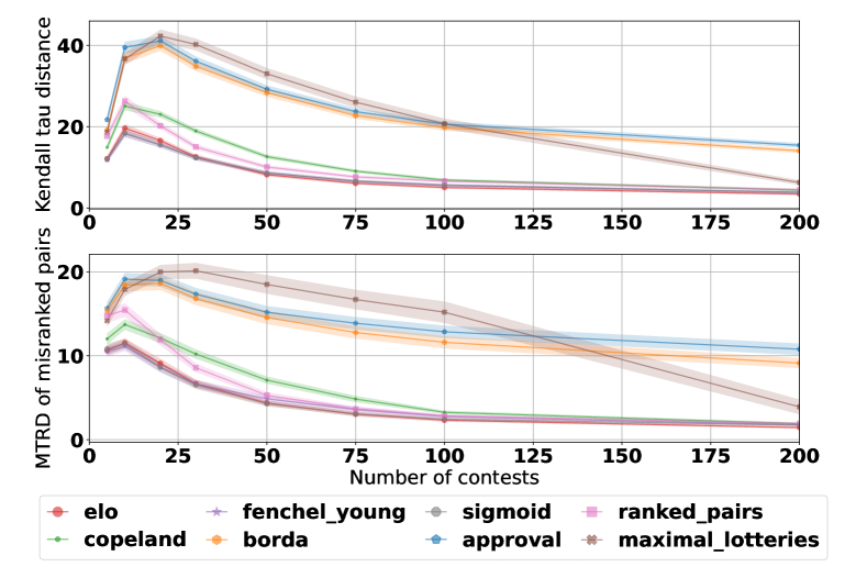
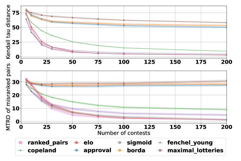
Figure 2: Kendall-tau distance (KTD) of ranking to true ranking, and Mean True Rating Distance (MTRD) of misranked pairs for ranking methods in tournament settings. Top: uniform distribution, Bottom: skill-matched distribution. Error bars represent 95% confidence intervals.

Of the VasE voting methods: approval, Borda, and maximal lotteries have the highest KTD and MRTD, and struggle especially in the skill-matched distribution. This is unsurprising; for example, approval and Borda will naturally weight alternatives according to their representation in the data. Under both distributions, when 59% or more of the match-ups are missing, SCO ratings (computed using both sigmoid and Fenchel-Young losses) achieve the lowest KTD and MRTD. Under the uniform distribution, SCO achieves the lowest when 38% or more of the data is missing. Under the skill-matched distribution, ranked pairs achieves comparable KTD to SCO ratings, and lower MRTD when the amount of missing data is less than 50%. Elo values are comparable to SCO in the uniform distribution and higher in the skill-matched distribution.

4.4 Diplomacy Game Outcome Prediction

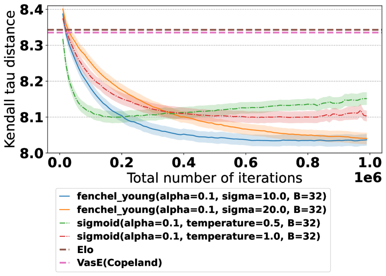
Figure 3: Average $\textsc{KTD}_{test}(t)$ between rankings and Diplomacy game outcomes across 50 seeds and train/test splits. All runs use batch size 32. Error bars depict 95% conf. intervals.

In this subsection we investigate the question of how well SCO rankings predict human game outcomes. Recall that this data set consists of all human-played seven-player games taken from the webDiplomacy.net spanning 11 years, resulting in a data set of size $m=52,958$ and $n=31,049$. As a result, less than $0.01\%$ of the unique player combinations are observed in the data. Finding a single ranking that sufficiently predicts the unseen test data is a difficult due to the extreme sparsity of the preference data.

We reflect the evaluation used in (Lanctot et al., 2023) with a small modification to adopt common practice in the supervised learning setting . First, we create 50 random splits of the data into training sets $\mathcal{D}_{R}$ and testing sets $\mathcal{D}_{T}$, with $|\mathcal{D}_{R}|=28049$ game outcomes (votes) and $|\mathcal{D}_{T}|=3000$ game outcomes. The random splits are such that each alternative in the test set is seen at least once on the training set, but no game outcomes (data points) are shared across train / test split. At each iteration $t$ the method has a ranking denoted $R_{t}$ learned from data in $\mathcal{D}_{R}$; we then compute and report the average Kendall-tau distance over the test set: $\textsc{KTD}_{test}(t)=\frac{1}{3000}\sum_{g\in\mathcal{D}_{T}}K_{d}(g,R_{t})$.

The resulting $\textsc{KTD}_{test}(t)$ is shown in Figure 3. We found that batch size had a minor effect on the results, so we show results for batch size 32 only. SCO with sigmoid loss reaches an average Kendall-tau distance of $8.10$ after roughly 190000 iterations, and Fenchel-Young loss reaches $8.05$ at 600000 iterations. There is an effect of increasing error after reaching this low point, likely due to overfitting; this could be reduced with early stopping, annealing learning rates, or other forms of regularization. As a point of comparison, Elo and the best VasE method on this data set, VasE(Copeland), achieve a value of $8.34$. The next best VasE method was plurality, achieving a value of 8.57. The more complex Condorcet methods, such as ranked pairs and maximal lotteries, cannot be run on this dataset due to their complexity, since $m=52,958$.

5 Discussion

The experimental results show various properties of SCO ratings, but which algorithm should be used to compute them in general? In our experience, sigmoidal programming produced similar results to standard gradient descent using the sigmoid loss; however, it sometimes suffered from numerical instability and was hard to scale to large number of agents due to programs requiring $m^{2}$ variables.

The Fenchel-Young loss is convex and hence gradient descent is guaranteed to converge to a global minimum; however, Condorcet winners (when they exist) are not necessarily top-ranked at that global minimum. Its practical performance is comparable to the sigmoid loss and slightly better in the large Diplomacy problem. Both the sigmoid and Fenchel-Young losses can be optimized online (batch size $|B|=1$) and work particularly well in approximating the optimal rankings when a large portion of evaluation data is missing and in complex ranking problem like Diplomacy.

This is further illustrated in Figure 4, where we plot two landscapes of the Fenchel-Young and sigmoid losses for the same data over three agents, using the example of vote profiles in Equation 10. Since both losses are invariant by adding a constant, we plot over a 2D slice, for all values of $\theta$ with the same sum. As discussed above, the Fenchel-Young loss is strictly convex, its global minimizer exists is found by gradient descent. Like Elo, it favours the win rate and assigns the highest rating not to the Condorcet winner $C$, but to $A$. In contrast, the sigmoid loss is nonconvex, and has no global minimizer (it keeps decreasing at infinity). Optimizing over constrained rating, it assigns the highest rating to the Condorcet winner $C$.

6 Conclusion and Future Work

We introduced Soft Condorcet Optimization, a ranking framework for general agents inspired by Condorcet’s original voting system criteria; it can be applied to agent-versus-task and agent-versus-agent evaluation problems, and more generally to any problem with ordinal preference data over a set of alternatives.

The optimum of the soft Kendall-tau (sigmoid) loss is guaranteed to top-rank Condorcet winners when they exist and in practice finds one most of the time when the number of alternatives $m\leq 500$. SCO ratings are closest to the optimal ranking when data is sparse, demonstrated both in a synthetic tournament setting with ground truth ratings and also in a challenge problem with thousands of human players in the board game of Diplomacy, a setting where the running complex Condorcet methods is computationally infeasible.

For future work, we would like to compare the performance of SCO to other learning-to-rank methods, to approximations of Kemeny (Kenyon-Mathieu and Schudy, 2007; Karpinski and Schudy, 2010; Ali and Meila, 2012) or other ranking methods inspired by tournament solutions (Rajkumar et al., 2015), or alternatives (Conati et al., 2022). Also, we would like to investigate using SCO as a reward model for post-training and alignment of language models (Conitzer et al., 2024).

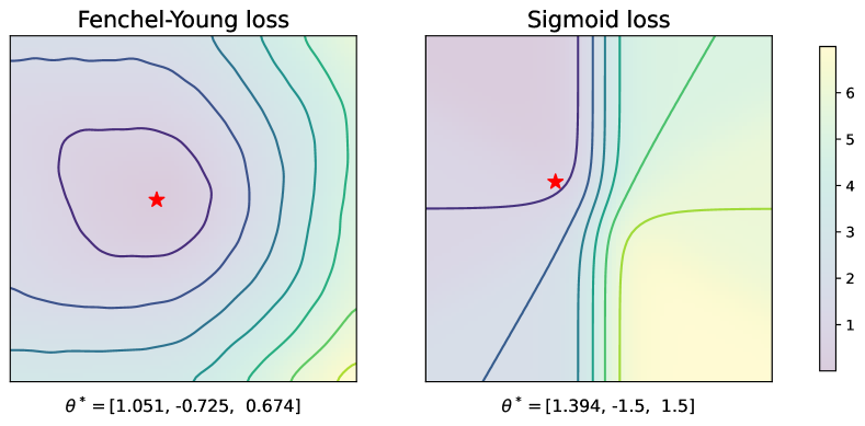
Figure 4: Loss landscapes for the Fenchel-Young (left) and sigmoid (right), with minimizer (red star) over $[-1.5,1.5]^{3}$.

Appendix A Proofs of Theorems

Recall that for a sigmoid $\sigma(x)=1-\sigma(-x)$ and the definitions of the $\mathbf{N}$ and $\mathbf{M}$ matrices from Section 2.3.

First, we will introduce some helpful notation and state a few facts. For a set of alternatives $A=\{a,b,\cdots\}$ and any ranking (total order) $R$ let $a\succ b\in A$ refer to the set of combinations where the left alternative is ranked higher the right alternative:

$$\{(a,b)\in A\times A\leavevmode\nobreak\ |\leavevmode\nobreak\ a\succ b\}.$$

This ranking can be arbitrary and need not refer to one returned by a social welfare function; e.g., for $A=\{a_{1},a_{2},\cdots,a_{m}\}$, then one natural ranking is by numerical indices so that

$$a\succ b\in A=\{(a_{1},a_{2}),(a_{1},a_{3}),\leavevmode\nobreak\ \cdots\leavevmode\nobreak\ ,(a_{1},a_{m}),(a_{2},a_{3}),(a_{2},a_{4}),\leavevmode\nobreak\ \cdots`,(a_{2},a_{m}),(a_{3},a_{4}),\leavevmode\nobreak\ \cdots\leavevmode\nobreak\ ,(a_{m-1},a_{m})\}.$$

When the ranking is not clear from the context, assume any default ranking is used to enumerate all combinations of size two.

Recall that the soft Kendall-tau loss (equation 6) can be expressed as a sum of sigmoids multiplied by coefficients from the $N$ matrix (equation 8). $\tilde{L}$ can be rewritten instead in terms of $M$:

$$\tilde{L}([\succeq],A,V,\bm{\theta}) = \sum_{a,b\in A\times A}N(a,b)\sigma(\theta_{b}-\theta_{a})$$

$$= \sum_{a\succ b\in A}[N(a,b)\sigma(\theta_{b}-\theta_{a})+N(b,a)\sigma(\theta_{a}-\theta_{b})]\text{\hskip 56.9055pt since }\forall a\in A,N(a,a)=0$$

$$= \sum_{a\succ b\in A}[N(a,b)\sigma(\theta_{b}-\theta_{a})+N(b,a)(1-\sigma(\theta_{b}-\theta_{a})]\text{\hskip 56.9055pt since }\sigma(x)=1-\sigma(-x)$$

$$= \sum_{a\succ b\in A}[N(b,a)+(N(a,b)-N(b,a))\sigma(\theta_{b}-\theta_{a})]$$

$$= \sum_{a\succ b\in A}N(b,a)+\sum_{a\succ b\in A}M(a,b)\sigma(\theta_{b}-\theta_{a}).$$

We now restate and prove the Theorem 1.

Theorem 1.

Given the sum of soft Kendall-tau distances:

$$\tilde{L}([\succeq],A,V,\bm{\theta}) = \sum_{a,b\in A\times A}N(a,b)\sigma(\theta_{b}-\theta_{a})\,.$$ (11)

If for preference profile $[\succ]$, voters $V$, there exists a candidate $c\in A$ that is a Condorcet winner, the loss is monotonically decreasing with $\theta_{c}$. As a consequence, if $\bm{\theta}^{*}$ is a global minimum of $\tilde{L}$ on the $\ell_{\infty}$ ball of radius $\theta_{\max}$, then $\theta^{*}_{c}=\theta_{\max}$.

Proof of Theorem 1.

Without loss of generality, we assume that $c\in A$ is the first element in some arbitrary order, and we rewrite the loss as

$$\tilde{L}([\succeq],A,V,\bm{\theta}) = K+\sum_{a\succ b\in A}M(a,b)\sigma(\theta_{b}-\theta_{a}),$$ (12)

where $K$ is a constant that does not depend on $\bm{\theta}$, as seen above. Since $c\succ b$ for all $b\in A$, we rewrite this loss as

$$\tilde{L}([\succeq],A,V,\bm{\theta}) = K+\sum_{b\in A}M(c,b)\sigma(\theta_{b}-\theta_{c})+\sum_{a\succ b\in A_{-c}}M(a,b)\sigma(\theta_{b}-\theta_{a})\,,$$ (13)

where $A_{-c}$ is the set of all candidates except $c\in A$. Note that the first term is a constant that does not depend on $\bm{\theta}$. The second term is monotonically decreasing in $\theta_{c}$, since $M(c,b)>0$ for all $b\in A_{-c}$ since $c$ is a Condorcet winner, and $\sigma$ is an increasing function. Further, the third term does not depend on $\theta_{c}$. As a consequence, for any vector $\theta$, increasing $\theta_{c}$ while leaving all other ratings equal decreases the loss.

As a consequence, if $\bm{\theta}^{*}$ is a global minimum on the $\ell_{\infty}$ ball of radius $\theta_{\max}$, $\theta^{*}_{c}=\theta_{\max}$. Indeed, if we had $\theta^{*}_{c}<\theta_{\max}$, increasing $\theta^{*}_{c}$ would decrease the loss, leading to a contradiction. ∎

This result shows that if there exists a Condorcet winner, there is no global minimum of $\mathbb{R}^{|A|}$ of the loss, since it is always better to increase $\theta_{c}$. It also shows that for any vector of ratings $\theta_{-c}$, the loss is smaller for $\theta_{c}\geq\max_{a\in A_{-c}}\theta_{a}$ than if $c$ did not have one of the highest ratings.

When there are constraints on $\bm{\theta}$, depending on the specific constraints, this can lead to several global minimizers. There can be several candidates with a rating of $\theta_{\max}$, even if only one of them is a Condorcet winner.

Appendix B Solving a Sigmoidal Program to Compute SCO Ratings

Recall, from Section 3.2.2:

$$\tilde{L}([\succeq],A,V,\bm{\theta}) = \sum_{a,b\in A\times A}N(a,b)\sigma(\theta_{b}-\theta_{a})$$

A sigmoidal program (Udell and Boyd, 2014) has the form:

minimize $$\sum_{i}f_{i}(x_{i})$$

subject to $$\mathbf{A}\mathbf{x}\leq\mathbf{b}$$

$$\mathbf{C}\mathbf{x}=\mathbf{d}$$

$$l\leq x_{i}\leq u,$$

whose objective is a sum of sigmoidal functions $f_{i}(x)$, defined as functions which are strictly convex on domain $x\leq z$ and then strictly concave on $x\geq z$ (i.e., $z=0$ in our case). Note that $N(a,b)\geq 0$ for all $a,b\in A$.

Each variable $x_{i}$ corresponds to $\theta_{a}-\theta_{b}$, for $a,b\in A,a\not=b$, so there are $|A|(|A|-1)=\Omega(m^{2})$ variables. The difference is lower-bounded by the parameter value range, so $u=\theta_{max}-\theta_{min}$ and $l=-u$.

There are no inequality constraints so $\mathbf{A}=0$ and $\mathbf{b}=0$. There are two types of equality constraints that are represented by $\mathbf{C}$ and $\mathbf{d}$:

• Constraints of the form $x_{i}+x_{j}=0$ representing the fact that $(\theta_{b}-\theta_{a})+(\theta_{a}-\theta_{b})=0$.

• Constraints to encode transitivity of the form $(\theta_{b}-\theta_{a})+(\theta_{a}-\theta_{c})=\theta_{b}-\theta_{c}.$

Appendix C Relationships between SCO and Prior Work

C.1 Relationship between SCO and Probabilistic Ranking

The problem of selecting an ordering that satisfies voters’ preferences has also been studied in statistics and psychology through probabilistic models defined over the space of permutations (Diaconis, 1988; Marden, 1995; Alvo and Yu, 2014). In particular, distance-based models (Fligner and Verducci, 1986) assume that voters have a true, collective preference over alternatives, $v^{*}$, and that the probability of observing any individual preference, $v\in V\subseteq[\succeq]$, is proportional to its distance from $v^{*}$. Thus, the probability of any individual vote $v\in V$ is

$$p(v)\propto\text{exp}(-K(v,v^{*}))$$ (14)

where $K$ is some metric between rankings.

Abusing notation slightly, let $p^{*}(v)$ and $p_{\bm{\theta}}(v)$ be the distance-based probability distributions induced by equation (14) for true collective ranking $v^{*}$ and some ranking $v_{\bm{\theta}}$ induced by parameters $\bm{\theta}$. To minimize the KL divergence between the true and parameterized distributions

$$\min_{\bm{\theta}}D_{KL}(p^{*}(v)||p_{\theta}(v)),$$ (15)

we maximize the likelihood of the rankings under the observed rankings or votes $v\in V$ by optimizing the MLE objective:

$$\min_{\bm{\theta}}\mathbb{E}_{v\sim p^{*}(v)}\left[K(v,v_{\bm{\theta}})\right].$$ (16)

When $K=K_{d}$ is the Kendall-tau distance and we apply the smooth approximation in equation (5), we recover the SCO objective:

$$\min_{\bm{\theta}}\frac{1}{|V|}\sum_{v\in V}\left[\sum_{(a,b)\in\binom{m}{2}}\sigma(\bm{\theta}_{a}-\bm{\theta}_{b})\right].$$ (17)

Since SCO falls within the class of distance-based models, it inherits a number of desirable properties, including strong unimodality (Critchlow et al., 1991; Alvo and Yu, 2014). This property states that if a true collective preference $v^{*}$ exists, then the probability of any preference $v$ is non-increasing as it moves away from $v^{*}$, with the ramification being that the MLE retrieves this unique (modal) ranking. On the other hand, for other probabilistic models, such as the pairwise comparison models which include Bradley-Terry and Elo (Bradley and Terry, 1952; Elo, 1978; Hunter, 2004), strong unimodality is not guaranteed in general, and instead requires (strong) stochastic transitivity among pairwise individual preferences (Critchlow et al., 1991; Alvo and Yu, 2014; Shah and Wainwright, 2018), a property that it not always observed in agent evaluation data (Bertrand et al., 2023; Boubdir et al., 2023).

C.1.1 Elo and Probablistic Rankings

As mentioned, Elo can be interpreted as an example of a pairwise-comparison based probabilistic ranking model. Since Elo is heavily used in the agent-evaluation context, we believe it is useful to fully illustrate this connection. This also allows us to further make a clear distinction between SCO and Elo.

A complete preference $v\in[\succeq]$ over the set of alternatives $A$ contains $\binom{|A|}{2}$ pairwise comparisons. Let the $\binom{|A|}{2}$ Bernoulli-distributed random variables $\bm{X}=\{X_{1},\ldots,X_{\binom{|A|}{2}}\}$ denote the outcome of observing every pairwise comparison on $v$. Each random variable $X_{k}$ represents the probability that alternative $a\in A$ is (strictly) preferred over alternative $b$. Thus, every Bernoulli parameter $p_{i}$ models the probability $p(a\succ b)$ as $p(x_{k}=1)=p_{k}$ and the converse preference $p(b\succ a)$ as $p(x_{k}=0)=1-p_{k}$. Pairwise comparison models (Bradley and Terry, 1952; Critchlow et al., 1991) assume that preferences between pairs of alternatives relate to their ratings $\bm{\theta}$ as:

$$p(a\succ b) =p(x_{k}=1)=p_{k}=\sigma(\bm{\theta}_{a}-\bm{\theta}_{b})$$

$$p(b\succ a) =p(x_{k}=0)=1-p_{k}=1-\sigma(\bm{\theta}_{a}-\bm{\theta}_{b})=\sigma(\bm{\theta}_{b}-\bm{\theta}_{a})$$

Given this framework and letting $p^{*}(\bm{X})$ model the true joint probability distribution of observing the $\binom{|A|}{2}$ pairwise rankings, and $p_{\bm{\theta}}(\bm{X})$ be the joint probability distribution induced by ratings $\bm{\theta}$, minimizing the KL divergence

$$\min_{\theta}D_{KL}\left(p^{*}(\bm{X})\big{\|}p_{\bm{\theta}}(\bm{X})\right)$$ (18)

and assuming the independence of the observed pairwise comparisons, is equivalent to minimizing the negative log-likelihood:

$$\min_{\bm{\theta}}\sum_{k=1}^{\binom{|A|}{2}}\mathbb{E}_{x_{k}\sim p^{*}(X_{k})}\left[-\log p_{\bm{\theta}}(x_{k})\right]$$ (19)

When optimized over some set of votes $v\in V\subseteq[\succeq]$ this leads to the objective:

$$\min_{\bm{\theta}}\frac{1}{|V|}\sum_{v\in V}\sum_{i=1}^{\binom{|A|}{2}}\mathbb{E}_{x_{k}\sim p^{*}(X_{k})}\left[-\log p_{\bm{\theta}}(x_{k})\right].$$ (20)

C.2 Relationship between SCO and Elo

Before we show the relation between SCO and Elo, we first summarize a well-known relationship between Elo and logistic regression (Morse, 2019).

Suppose player $i$ plays player $j$ and the outcome is $y_{ij}=1$ if $i$ won and $0$ otherwise. Recall from that Elo’s online update rule is:

$$\theta_{i}\leftarrow\theta_{i}+K(y_{ij}-p_{ij}),$$ (21)

where

$$p_{ij}=\frac{1}{1+10^{(\theta_{j}-\theta_{i})/400}}$$

is Elo’s predicted probability (of agent $i$ beating agent $j$), and $K=32$ (Elo, 1978). Logistic regression is a method for classification that models the prediction as a logistic function of a linear function between parameters and features (Cramer, 2002; Murphy, 2022). In binary classification, data points $(\mathbf{x},y)$ comprise input vectors $\mathbf{x}$ and classes $y\in\{0,1\}$. Define the log odds of the data point given a label of 1:

$$\textsc{LogOdds}(\mathbf{x},y=1)=\log_{10}\left(\cdot\frac{\Pr(\mathbf{x}\leavevmode\nobreak\ |\leavevmode\nobreak\ y=1)\Pr(y=1)}{\Pr(\mathbf{x}\leavevmode\nobreak\ |\leavevmode\nobreak\ y=0)\Pr(y=0)}\right).$$

The probability of class 1 for a given $\mathbf{x}$ is (via Bayes’ rule) is

$$\Pr(y=1\leavevmode\nobreak\ |\leavevmode\nobreak\ \mathbf{x}) = \frac{\Pr(\mathbf{x}|y=1)\Pr(y=1)}{\Pr(\mathbf{x}|y=1)\Pr(y=1)+\Pr(\mathbf{x}|y=0)\Pr(y=0)}$$

$$= \frac{1}{1+\frac{\Pr(\mathbf{x}|y=0)\Pr(y=0)}{\Pr(\mathbf{x}|y=1)\Pr(y=1)}}$$

$$= \frac{1}{1+10^{\textsc{LogOdds}(\mathbf{x},y=1)/400}}.$$

Let $p_{k}$ be the probability predicted by the model for data point $(\mathbf{x}_{k},y_{k})$. The standard loss (error) used for a data point $(\mathbf{x}_{k},y_{k})$ is a log loss $\ell_{k}=-\log p_{k}$ if $y_{k}=1$ and $-\log(1-p_{k})$ if $y_{k}=0$, which is combined into a single loss term:

$$\ell_{k}=-y_{k}\log p_{k}-(1-y_{k})\log(1-p_{k}),$$ (22)

and the loss over a data set of $K$ examples is $\ell=\sum_{k=1}^{K}\ell_{k}$. The prediction is modeled using parameters $\bm{\theta}$ such that $p_{k}=\sigma(\bm{\theta}^{T}\mathbf{x}_{k})$. The derivative of the sigmoid is conveniently $\frac{d}{dx}\sigma(x)=\sigma(x)(1-\sigma(x))$, so the gradient of the loss for point $k$ turns out to be:

$$\nabla_{\bm{\theta}}\ell_{k}=(\sigma(\bm{\theta}^{T}\mathbf{x}_{k})-y_{k})\mathbf{x}_{k}.$$ (23)

Here, $\bm{\theta}$ represents the Elo ratings and the data points (game outcomes), $\mathbf{x}_{k}$, contain all zeros except 1 for the player who won and -1 for the player who lost. Now, the gradient descent update rule is: $\bm{\theta}\leftarrow\bm{\theta}-\alpha\nabla_{\bm{\theta}}\ell_{k}$; the update in Equation 23 is proportional to Equation 21. To see this, when $i$ beats $j$ and $y_{k}=1$, then

$$-\alpha\nabla_{\bm{\theta}}\ell_{k} = (\sigma(\bm{\theta}^{T}\mathbf{x}_{k})-1)\mathbf{x}_{k}$$

$$= -\alpha(\sigma(\theta_{i}-\theta_{j})-1)\mathbf{x}_{k}$$

$$= +\alpha(1-\sigma(\theta_{i}-\theta_{j}))\mathbf{x}_{k},$$

and due to the definition of $x_{k}$ will result in the magnitude being added to $\theta_{i}$ and subtracted from $\theta_{j}$.

How, then, does SCO relate to Elo? As in SCO, the Elo ratings are the parameters of the model and the loss is a function of the difference in ratings passed through a logistic function. The key difference is the loss function used. In Elo, the gradient update is derived from fitting a classifier to predict the probability of a win given two agents’ ratings. As such, the standard negative log-likelihood is used (Murphy, 2022). In SCO, the loss is the sum of sigmoids represented as $D_{v}$ (equation (6) and equation (5)) itself, specifically because it is interpreted as a (smooth) Kendall-tau distance– the optimal point being its minimum– rather than as a prediction.

C.3 Relationship to Perturbed Optimizers

A variety of methods have been considered to produce smooth proxys of ranking operators, i.e. functions that approximate a ranking or sorting function, that are differentiable (see, e.g. (Blondel et al., 2020b) and references therein). Indeed ranking is just one type of discrete-output operation that can be efficiently made differentiable, and we describe here the approach of (Berthet et al., 2020) following their notation: consider a general discrete optimization problem over a set $\mathcal{Y}$ that can be parameterized by an input $\bm{\theta}\in\mathbb{R}^{m}$, for a finite set of distinct points $\mathcal{Y}\subset\mathbb{R}^{m}$ with $\mathcal{C}$ being its convex hull, of the form:

$$F(\bm{\theta})=\max_{\mathbf{y}\in\mathcal{C}}\mathbf{y}^{T}\bm{\theta},\mbox{\leavevmode\nobreak\ \leavevmode\nobreak\ and\leavevmode\nobreak\ \leavevmode\nobreak\ }\mathbf{y}^{*}(\bm{\theta})=\operatornamewithlimits{argmax}_{\mathbf{y}\in\mathcal{C}}\mathbf{y}^{T}\bm{\theta}.$$ (24)

In particular, consider the case where $\mathcal{C}$ is a convex polytope and the problems are linear programs. As an example, the problem of ranking a vector of $d$ entries can be cast in this fashion, by taking $C$ to be the permutahedron $\mathcal{P}(\rho)$ (see below). The function $\mathbf{y}^{*}:\mathbb{R}^{d}\to\mathcal{Y}$ is piecewise constant, leading to zero or undefined gradients. It can be smoothed by taking the mean under additive stochastic noise to the parameters: we define this proxy by the perturbed maximizer (Berthet et al., 2020) for $\varepsilon>0$

$$\mathbf{y}^{*}_{\varepsilon}(\bm{\theta})=\mathbb{E}_{Z}[y^{*}(\bm{\theta}+\varepsilon Z)]=\mathbb{E}_{Z}[\operatornamewithlimits{argmax}_{y\in\mathcal{C}}\mathbf{y}^{T}(\bm{\theta}+\varepsilon Z)]\,,$$ (25)

where $Z$ is a random variable with a positive and differentiable density. Under these conditions, the argmax inside the expectation is almost surely unique, and $\mathbf{y}^{*}_{\varepsilon}$ is differentiable, with derivatives that are also expressed as a mean, and that can be estimated with Monte-Carlo methods (see (Berthet et al., 2020)). Further, one can define the probability distribution $p_{\bm{\theta}}(y)=\Pr(\mathbf{y}^{*}(\bm{\theta}+\varepsilon Z)=y)$. It holds that $\mathbf{y}^{*}_{\varepsilon}(\bm{\theta})=\mathbb{E}_{p_{\bm{\theta}}(y)}[Y]$, and the perturbed maximum is

$$F_{\varepsilon}(\bm{\theta})=\mathbb{E}[F(\bm{\theta}+\varepsilon Z)]=\mathbb{E}[\mathbf{y}^{*}(\bm{\theta}+\varepsilon Z)^{\top}(\bm{\theta}+\varepsilon Z)].$$ (26)

The ranking operation for some vector of values $\mathbf{v}$ can be seen as Ranking$(\mathbf{v})=\textsc{ArgSort}(\textsc{ArgSort}(\mathbf{v}))$, where ArgSort is a function that returns the indices that would sort the values. It is precisely this non-differentiable function that will be perturbed. For example, for $\mathbf{v}=(0.18,-1.28,0.65,1.25,0.25,-0.12)$,

$$\textsc{Ranking}(\mathbf{v})=(2,0,4,5,3,1).$$

Ranking can be cast as an LP in the form required by equation (24). Let $\mathcal{P}(\mathbf{w})$ be the permutahedron: the convex hull over all vectors that are permutations of $\mathbf{w}\subset\mathbb{R}^{m}$. For $\rho=(m,\cdots,1)$, a (linear) objective function is constructed that is the dot product of $-\bm{\theta}$ and $\mathbf{y}\in\mathcal{P}(\rho)$. The fundamental theorem of linear programming ensures that the solution of an LP is vertex of it polytope, unique for almost all inputs, corresponding to a permutation in the case of a permutahedron (Berthet et al., 2020). As an example, suppose the ratings for agents $1,2,3,4$ are $(10,20,30,40)$. Then the maximum objective would be when $\mathbf{y}=\rho$ with a maximal value of $(4,3,2,1)\cdot(-10,-20,-30,-40)$. These methods learn such ranking functions from data via gradient descent. Indeed $\mathbf{y}_{\varepsilon}^{*}(\bm{\theta})$ can be plugged in directly into any loss $\ell$ comparing it to a vector of ranks $\mathbf{y}_{\text{true}}$. Further, the formalism of Fenchel-Young losses (Blondel et al., 2020a) can be applied to this setting: they are particularly convenient to use with perturbed optimizer, as their gradient is given by

$$\nabla_{\theta}\ell_{\text{FY}}(\theta;\mathbf{y}_{\text{true}})=\mathbf{y}_{\varepsilon}^{*}(\theta)-\mathbf{y}_{\text{true}}\,.$$

As detailed in our main text, this can be extended naturally to partial rankings, and constructing stochastic gradients based on batches of these rankings. The connection to SCO is clear. In perturbed optimizers, the user explicitly chooses the distribution of $Z$ (e.g., Gumbel or Normal) and fits parameters $\bm{\theta}$ to the data under the model given by equation (25). In Young’s formalization of Condorcet’s model, the noise follows the Mallows model where the probability of a data point is proportional to its Kendall-tau distance to the ground truth rankings.

Appendix D Additional Results and Hyper-Parameter Values

D.1 Full SCO Results on the Failure Mode of Elo

Table 4 shows the full results for of all hyperparameters used for the warmup experiment described in Section 4.1.

Full vs. Stochastic Gradient Descent	$\alpha$	$\tau$	$T_{conv}$
GD	$0.01$	$0.5$	$289$
GD	$0.01$	$1$	$1158$
GD	$0.01$	$2$	$4661$
GD	$0.1$	$0.5$	$28$
GD	$0.1$	$1$	$115$
GD	$0.1$	$2$	$463$
SGD ($|B|=2$)	$0.01$	$0.5$	$17.0$
SGD ($|B|=2$)	$0.01$	$1$	$1003.33$
SGD ($|B|=2$)	$0.01$	$2$	$4778.33$
SGD ($|B|=2$)	$0.1$	$0.5$	$25.00$
SGD ($|B|=2$)	$0.1$	$1$	$60.66$
SGD ($|B|=2$)	$0.1$	$2$	$401.66$

Table 4: Number of iterations to reach convergence to the optimal ranking on the example in Equation 10. $\alpha$ is the learning rate and $\tau$ is the temperature of the logistic function (Equation (5)). $T_{conv}$ is the number of iterations required to converge to the optimal ranking; for SGD this is an average over 3 seeds.

D.2 Kemeny-Young Approximation Quality

For the results listed across PrefLib instances from Table 2:

• For sigmoidal programming, we used maxiters of 10000. The tolerance parameter was first set to 0.0001. If a numerical instability occurred, then the problem was retried with a tolerance of 0.001 and then if that failed again, then 0.01 was used.

• For instances where $m\leq 10$, SGD with the sigmoid loss used batch size of 32, 10000 iterations, $\alpha=0.01$, and temperature $\tau=1$.

• For instances where $11\leq m\leq 500$, SGD with the sigmoid loss used batch size 32, 100000 iterations, $\alpha=0.01$, and temperature $\tau=1$.

• For instances where $m\geq 501$, SGD with the sigmoid loss used batch size 32, 100000 iterations, $\alpha=0.1$, and temperature $\tau=\frac{1}{2}$.

D.3 Approximation of Bayesian Posterior

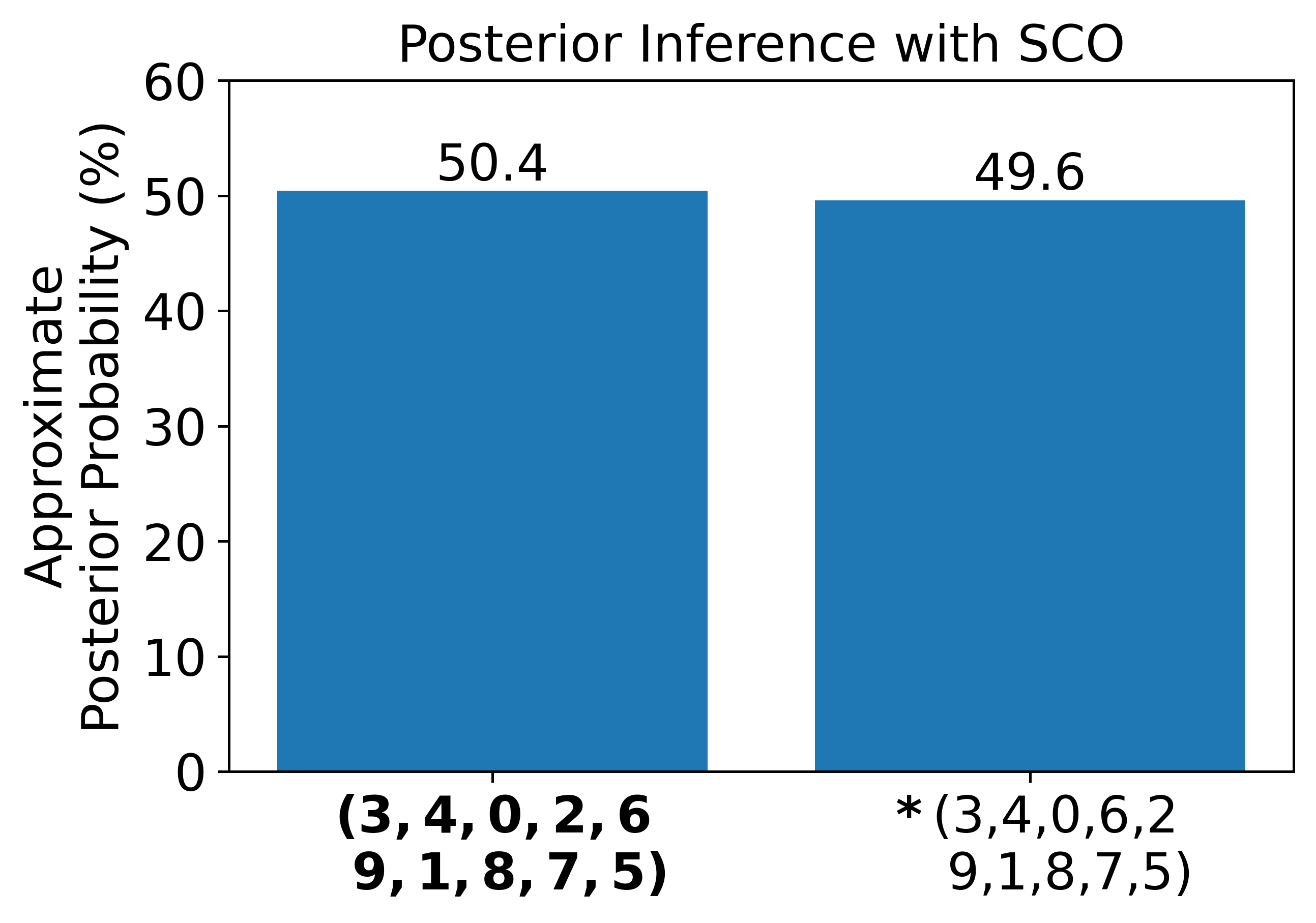
Figure 5: Posterior inference via Algorithm 1 on a synthetic evaluation problem. Contests between $4$ participants are randomly drawn from a pool of $10$. The ranking of the final rating $\theta_{T}$ is denoted with an asterisk (*). The true skill ranking is labeled in bold. True skills ratings, to two decimal places, are $[126.46,106.00,114.68,133.61,128.01,85.34,114.25,97.73,98.45,$ $106.16]$. All rankings sampled from the SGD-as-posterior-inference process are labeled in the bar plot with their corresponding observed frequencies as probabilities displayed above them. Notice that the mode of the posterior matches the true skill ranking and improves upon the final iterate.

Prior work (Mandt et al., 2016; Stephan et al., 2017) has shown how stochastic gradient descent (SGD) can be modified to go beyond an MLE point estimate and approximately generate samples from the Bayes posterior of a probabilistic model. Under assumptions that SGD has converged to a region around a local minimum where the loss is quadratic and gradients are normally distributed, a new optimal step size can be computed from gradient samples.

Here, we show this using Algorithm 1 with a constant learning rate, on simulated rank data generated similarly to the skill-matched distribution in Section 4.3, but with $m=10$. Once SCO has converged to a region, a new optimal step size is computed using gradient samples. As SGD continues with this new step size, it traverses the stationary distribution of a Markov chain and produces iterates that well approximate samples from the true posterior distribution (see Figure 5). While the posterior over ratings $\bm{\theta}$ is assumed Gaussian, the induced distribution over rankings could be multimodal. Moreover, probabilities over rankings can provide uncertainty estimates to specific alternatives in the rankings.

Figure 5 displays the posterior over rankings. In this case, the true ratings for agents $2$ and $6$ are $114.68$ and $114.25$ respectively. These are the most closely rated agents in the game. The posterior distribution reflects the uncertainty in how to rank these two agents when observing noisy outcomes of their contests.

D.4 Online Performance

We now evaluate the performance of SCO in the online setting. In the online setting, the data is presented to each method as a stream: one data point at a time. The ranking method must update its parameters incrementally using only the one data point. The online form of SCO is obtained simply by running one stochastic gradient descent update on the data point (batch of size 1). One advantage of Elo is that its online update involves updating only the ratings of players involved in the game that was played, so it can be employed in a decentralized way after each game. SCO shares this advantage because the gradients of the batch $\nabla_{\bm{\theta}}L(B)$ involve only those players that were present in $B$. For SCO, we use the same setup and evaluation metric as in Section 4.4, except using batch size 1 and only one single pass over training data points, leading to a total number of iterations $T=|\mathcal{D}_{R}|=28049$. We run 50 such experiments with different seeds corresponding to 50 different orderings of the data. The results are shown in Figure 6.

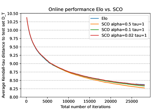
Figure 6: Online performance of SCO. Bands around each line represent 95% confidence intervals over 50 runs.

We tried $\alpha\in\{0.5,0.2,0.1,0.02,0.01\}$ and temperatures $\tau\in\{0.5,1,2\}$. The results were quite comparable, so we show only the extremes in variation for $\tau=1$. In this case SCO with $\alpha=0.02$ most closely resembles Elo while SCO with $\alpha=0.1$ preforms slightly better than Elo and $\alpha=0.5$ significantly better.

References

- Ali and Meila (2012) A. Ali and M. Meila. Experiments with kemeny ranking: What works when? Mathematical Social Sciences, 64(1):28–40, 2012.
- Alvo and Yu (2014) M. Alvo and P. L. H. Yu. Statistical Methods for Ranking Data. Springer New York, Sept. 2014.
- Aziz et al. (2015) H. Aziz, M. Brill, F. Fischer, P. Harrenstein, J. Lang, and H. G. Seedig. Possible and necessary winners of partial tournaments. Journal of Artificial Intelligence Research, 54:493–534, 2015.
- Baid et al. (2023) G. Baid, D. E. Cook, K. Shafin, T. Yun, F. Llinares-López, Q. Berthet, A. Belyaeva, A. Töpfer, A. M. Wenger, W. J. Rowell, et al. Deepconsensus improves the accuracy of sequences with a gap-aware sequence transformer. Nature Biotechnology, 41(2):232–238, 2023.
- Balduzzi et al. (2018) D. Balduzzi, K. Tuyls, J. Perolat, and T. Graepel. Re-evaluating evaluation. In S. Bengio, H. Wallach, H. Larochelle, K. Grauman, N. Cesa-Bianchi, and R. Garnett, editors, Advances in Neural Information Processing Systems, volume 31. Curran Associates, Inc., 2018.
- Bellemare et al. (2013) M. G. Bellemare, Y. Naddaf, J. Veness, and M. Bowling. The arcade learning environment: An evaluation platform for general agents. Journal of Artificial Intelligence Research, 47:253–279, jun 2013.
- bench authors (2023) B. bench authors. Beyond the imitation game: Quantifying and extrapolating the capabilities of language models. Transactions on Machine Learning Research, 2023. ISSN 2835-8856. URL https://openreview.net/forum?id=uyTL5Bvosj.
- Berthet et al. (2020) Q. Berthet, M. Blondel, O. Teboul, M. Cuturi, J.-P. Vert, and F. Bach. Learning with differentiable pertubed optimizers. In H. Larochelle, M. Ranzato, R. Hadsell, M. Balcan, and H. Lin, editors, Advances in Neural Information Processing Systems, volume 33, pages 9508–9519. Curran Associates, Inc., 2020. URL https://proceedings.neurips.cc/paper_files/paper/2020/file/6bb56208f672af0dd65451f869fedfd9-Paper.pdf.
- Bertrand et al. (2023) Q. Bertrand, W. M. Czarnecki, and G. Gidel. On the limitations of the elo, Real-World games are transitive, not additive. In F. Ruiz, J. Dy, and J.-W. van de Meent, editors, Proceedings of The 26th International Conference on Artificial Intelligence and Statistics, volume 206 of Proceedings of Machine Learning Research, pages 2905–2921. PMLR, 2023.
- Blondel et al. (2020a) M. Blondel, A. F. Martins, and V. Niculae. Learning with Fenchel-Young losses. The Journal of Machine Learning Research, 21(1):1314–1382, 2020a.
- Blondel et al. (2020b) M. Blondel, O. Teboul, Q. Berthet, and J. Djolonga. Fast differentiable sorting and ranking. In H. D. III and A. Singh, editors, Proceedings of the 37th International Conference on Machine Learning, volume 119 of Proceedings of Machine Learning Research, pages 950–959. PMLR, 13–18 Jul 2020b. URL https://proceedings.mlr.press/v119/blondel20a.html.
- Boubdir et al. (2023) M. Boubdir, E. Kim, B. Ermis, S. Hooker, and M. Fadaee. Elo uncovered: Robustness and best practices in language model evaluation. Nov. 2023.
- Bradley and Terry (1952) R. A. Bradley and M. E. Terry. Rank analysis of incomplete block designs I: The method of paired comparisons. Biometrika, 39:324–345, 1952.
- Brandt et al. (2016) F. Brandt, V. Conitzer, U. Endriss, J. Lang, and A. D. Procaccia, editors. Handbook of Computational Social Choice. Cambridge University Press, 2016.
- Campbell et al. (2002) M. Campbell, J. Hoane, A. Joseph, and F.-h. Hsu. Deep blue. Artificial Intelligence, 134(1–2):57–83, 2002.
- Carr et al. (2021) A. N. Carr, Q. Berthet, M. Blondel, O. Teboul, and N. Zeghidour. Self-supervised learning of audio representations from permutations with differentiable ranking. IEEE Signal Processing Letters, 28:708–712, 2021.
- Chiang et al. (2024) W.-L. Chiang, L. Zheng, Y. Sheng, A. N. Angelopoulos, T. Li, D. Li, B. Zhu, H. Zhang, J. E. G. Michael Jordan, and I. Stoica. Chatbot arena: An open platform for evaluating llms by human preference. In Proceedings of the 41st International Conference on Machine Learning, volume 235 of PLMR, 2024.
- Conati et al. (2022) A. Conati, A. Niskanen, and M. Järvisalo. Sat-based judgment aggregation. In International Conference on Autonomous Agents and Multiagent Systems (AAMAS), 2022.
- Conitzer and Sandholm (2005) V. Conitzer and T. Sandholm. Common voting rules as maximum likelihood estimators. In Proceedings of the Conference on Uncertainty in Artificial Intelligence (UAI), pages 145–152, 2005.
- Conitzer et al. (2024) V. Conitzer, R. Freedman, J. Heitzig, W. H. Holliday, B. M. Jacobs, N. Lambert, M. Mosse, E. Pacuit, S. Russell, H. Schoelkopf, E. Tewolde, and W. S. Zwicker. Position: Social choice should guide AI alignment in dealing with diverse human feedback. In R. Salakhutdinov, Z. Kolter, K. Heller, A. Weller, N. Oliver, J. Scarlett, and F. Berkenkamp, editors, Proceedings of the 41st International Conference on Machine Learning, volume 235 of Proceedings of Machine Learning Research, pages 9346–9360. PMLR, 21–27 Jul 2024. URL https://proceedings.mlr.press/v235/conitzer24a.html.
- Cordonnier et al. (2021) J.-B. Cordonnier, A. Mahendran, A. Dosovitskiy, D. Weissenborn, J. Uszkoreit, and T. Unterthiner. Differentiable patch selection for image recognition. In Proceedings of the Conference on Computer Vision and Pattern Recognition, pages 2351–2360, 2021.
- Coulom (2005) R. Coulom. Bayesian Elo rating, 2005. https://www.remi-coulom.fr/Bayesian-Elo.
- Cramer (2002) J. Cramer. The origins of logistic regression. Technical report, 2002.
- Critchlow et al. (1991) D. E. Critchlow, M. A. Fligner, and J. S. Verducci. Probability models on rankings. Journal of mathematical psychology, 35(3):294–318, Sept. 1991.
- Cuturi (2013) M. Cuturi. Sinkhorn distances: Lightspeed computation of optimal transport. Advances in Neural Information Processing Systems, 26, 2013.
- Cuturi and Blondel (2017) M. Cuturi and M. Blondel. Soft-DTW: a differentiable loss function for time-series. In International Conference on Machine Learning, pages 894–903, 2017.
- de Condorcet (1785) M. de Condorcet. Essai sur l’application de l’analyse à la probabilité des décisions rendues à la pluralité des voix, 1785.
- Diaconis (1988) P. Diaconis. Group representations in probability and statistics, volume 11 of Lecture Notes-Monograph Series. Institute of Mathematical Statistics, Jan. 1988.
- Dubois-Taine et al. (2022) B. Dubois-Taine, F. Bach, Q. Berthet, and A. Taylor. Fast stochastic composite minimization and an accelerated frank-wolfe algorithm under parallelization. In Advances in Neural Information Processing Systems, 2022.
- Elo (1978) A. E. Elo. The Ratings of Chess Players, Past and Present. Arco Publishing, Inc., 2nd edition, 1978.
- (31) M. F. A. R. D. T. (FAIR)†, A. Bakhtin, N. Brown, E. Dinan, G. Farina, C. Flaherty, D. Fried, A. Goff, J. Gray, H. Hu, A. P. Jacob, M. Komeili, K. Konath, M. Kwon, A. Lerer, M. Lewis, A. H. Miller, S. Mitts, A. Renduchintala, S. Roller, D. Rowe, W. Shi, J. Spisak, A. Wei, D. Wu, H. Zhang, and M. Zijlstra. Human-level play in the game of Diplomacy by combining language models with strategic reasoning. Science, 378(6624):1067–1074, 2022. 10.1126/science.ade9097. URL https://www.science.org/doi/abs/10.1126/science.ade9097.
- Fligner and Verducci (1986) M. A. Fligner and J. S. Verducci. Distance based ranking models. Journal of the Royal Statistical Society. Series B, Statistical methodology, 48(3):359–369, 1986.
- Gumbel (1954) E. J. Gumbel. Statistical Theory of Extreme Values and some Practical Applications: A Series of Lectures. Number 33. US Govt. Print. Office, 1954.
- Hazan (2015) E. Hazan. Introduction to online convex optimization. Now Publishers Inc., 2015. Foundations and Trends in Optimization, Volume 2, Issue 3-4.
- Hazan et al. (2016) T. Hazan, G. Papandreou, and D. Tarlow. Perturbations, Optimization, and Statistics. MIT Press, 2016.
- Herbrich et al. (2006) R. Herbrich, T. Minka, and T. Graepel. Trueskill™: A Bayesian skill rating system. In B. Schölkopf, J. Platt, and T. Hoffman, editors, Advances in Neural Information Processing Systems, volume 19. MIT Press, 2006.
- Hunter (2004) D. R. Hunter. MM algorithms for generalized Bradley-Terry models. The Annals of Statistics, 32(1):384–406, 2004.
- Karpinski and Schudy (2010) M. Karpinski and W. Schudy. Faster algorithms for feedback arc set tournament, kemeny rank aggregation and betweenness tournament. ISAAC, 6506:3–14, 2010.
- (39) M. Kelly, R. Longjohn, and K. Nottingham. The uci machine learning repository. https://archive.ics.uci.edu.
- Kemeny (1959) J. Kemeny. Mathematics without numbers. Daedalus, 88(4):577–591, 1959.
- Kenyon-Mathieu and Schudy (2007) C. Kenyon-Mathieu and W. Schudy. How to rank with few errors. In Proceedings of the Thirty-Ninth Annual ACM Symposium on Theory of Computing, STOC ’07, page 95–103, New York, NY, USA, 2007. Association for Computing Machinery. ISBN 9781595936318. 10.1145/1250790.1250806. URL https://doi.org/10.1145/1250790.1250806.
- Krizhevsky et al. (2012) A. Krizhevsky, I. Sutskever, and G. E. Hinton. Imagenet classification with deep convolutional neural networks. In Proceedings of the 25th International Conference on Neural Information Processing Systems, pages 1097–1105, 2012.
- Kumar et al. (2021) A. Kumar, G. Brazil, and X. Liu. Groomed-nms: Grouped mathematically differentiable nms for monocular 3d object detection. In Proceedings of the Conference on Computer Vision and Pattern Recognition, pages 8973–8983, 2021.
- Lanctot et al. (2023) M. Lanctot, K. Larson, Y. Bachrach, L. Marris, Z. Li, A. Bhoopchand, T. Anthony, B. Tanner, and A. Koop. Evaluating agents using social choice theory, 2023.
- Le Lidec et al. (2021) Q. Le Lidec, I. Laptev, C. Schmid, and J. Carpentier. Differentiable rendering with perturbed optimizers. Advances in Neural Information Processing Systems, 34:20398–20409, 2021.
- Liang et al. (2022) P. Liang, R. Bommasani, T. Lee, D. Tsipras, D. Soylu, M. Yasunaga, Y. Zhang, D. Narayanan, Y. Wu, A. Kumar, B. Newman, B. Yuan, B. Yan, C. Zhang, C. Cosgrove, C. D. Manning, C. Ré, D. Acosta-Navas, D. A. Hudson, E. Zelikman, E. Durmus, F. Ladhak, F. Rong, H. Ren, H. Yao, J. Wang, K. Santhanam, L. Orr, L. Zheng, M. Yuksekgonul, M. Suzgun, N. Kim, N. Guha, N. Chatterji, O. Khattab, P. Henderson, Q. Huang, R. Chi, S. M. Xie, S. Santurkar, S. Ganguli, T. Hashimoto, T. Icard, T. Zhang, V. Chaudhary, W. Wang, X. Li, Y. Mai, Y. Zhang, and Y. Koreeda. Holistic evaluation of language models. CoRR, abs/2211.09110, 2022. See latest results at: https://crfm.stanford.edu/helm/latest/.
- Liu (2011) T.-Y. Liu. Learning to Rank for Information Retrieval. Springer, 2011.
- Liu et al. (2023) X. Liu, H. Yu, H. Zhang, Y. Xu, X. Lei, H. Lai, Y. Gu, H. Ding, K. Men, K. Yang, S. Zhang, X. Deng, A. Zeng, Z. Du, C. Zhang, S. Shen, T. Zhang, Y. Su, H. Sun, M. Huang, Y. Dong, and J. Tang. Agentbench: Evaluating llms as agents, 2023.
- Llinares-López et al. (2023) F. Llinares-López, Q. Berthet, M. Blondel, O. Teboul, and J.-P. Vert. Deep embedding and alignment of protein sequences. Nature Methods, 20(1):104–111, 2023.
- Mandt et al. (2016) S. Mandt, M. Hoffman, and D. Blei. A variational analysis of stochastic gradient algorithms. In International conference on machine learning, pages 354–363. PMLR, 2016.
- Marden (1995) J. I. Marden. Analyzing and Modeling Rank Data. Chapman and Hall, 1995.
- Mattei and Walsh (2013) N. Mattei and T. Walsh. Preflib: A library of preference data http://preflib.org. In Proceedings of the 3rd International Conference on Algorithmic Decision Theory (ADT 2013), Lecture Notes in Artificial Intelligence. Springer, 2013.
- Mensch and Blondel (2018) A. Mensch and M. Blondel. Differentiable dynamic programming for structured prediction and attention. In Proc. of ICML, 2018.
- Morse (2019) S. Morse. Elo as a statistical learning model, 2019. https://stmorse.github.io/journal/Elo.html. Retrieved January 2024.
- Murphy (2022) K. P. Murphy. Probabilistic Machine Learning: An introduction. MIT Press, 2022. URL probml.ai.
- Paulus et al. (2020) M. Paulus, D. Choi, D. Tarlow, A. Krause, and C. J. Maddison. Gradient estimation with stochastic softmax tricks. Advances in Neural Information Processing Systems, 33:5691–5704, 2020.
- Pini et al. (2011) M. S. Pini, F. Rossi, K. B. Venable, and T. Walsh. Possible and necessary winners in voting trees: majority graphs vs. profiles. In The 10th International Conference on Autonomous Agents and Multiagent Systems-Volume 1, pages 311–318, 2011.
- Rajkumar et al. (2015) A. Rajkumar, S. Ghoshal, L.-H. Lim, and S. Agarwal. Ranking from stochastic pairwise preferences: Recovering condorcet winners and tournament solution sets at the top. In Proceedings of the 32nd International Conference on Machine Learning, volume 37 of Proceedings of Machine Learning Research, pages 665–673, 2015.
- Rofin et al. (2023) M. Rofin, V. Mikhailov, M. Florinsky, A. Kravchenko, T. Shavrina, E. Tutubalina, D. Karabekyan, and E. Artemova. Vote’n’rank: Revision of benchmarking with social choice theory. In A. Vlachos and I. Augenstein, editors, Proceedings of the 17th Conference of the European Chapter of the Association for Computational Linguistics, pages 670–686, Dubrovnik, Croatia, May 2023. Association for Computational Linguistics. 10.18653/v1/2023.eacl-main.48. URL https://aclanthology.org/2023.eacl-main.48.
- Samuel (1959) A. L. Samuel. Some studies in machine learning using the game of checkers. IBM Journal of Research and Development, 44:206–226, 1959.
- Sander et al. (2023) M. E. Sander, J. Puigcerver, J. Djolonga, G. Peyré, and M. Blondel. Fast, differentiable and sparse top-k: a convex analysis perspective. arXiv preprint arXiv:2302.01425, 2023.
- Shah and Wainwright (2018) N. B. Shah and M. J. Wainwright. Simple, robust and optimal ranking from pairwise comparisons. Journal of machine learning research: JMLR, 18(199):1–38, 2018.
- Silver et al. (2016) D. Silver, A. Huang, C. J. Maddison, A. Guez, L. Sifre, G. van den Driessche, J. Schrittwieser, I. Antonoglou, V. Panneershelvam, M. Lanctot, S. Dieleman, D. Grewe, J. Nham, N. Kalchbrenner, I. Sutskever, T. Lillicrap, M. Leach, K. Kavukcuoglu, T. Graepel, and D. Hassabis. Mastering the game of Go with deep neural networks and tree search. Nature, 529:484–489, 2016.
- Silver et al. (2018) D. Silver, T. Hubert, J. Schrittwieser, I. Antonoglou, M. Lai, A. Guez, M. Lanctot, L. Sifre, D. Kumaran, T. Graepel, T. Lillicrap, K. Simonyan, and D. Hassabis. A general reinforcement learning algorithm that masters chess, shogi, and Go through self-play. Science, 632(6419):1140–1144, 2018.
- Smith (1973) J. H. Smith. Aggregation of preferences with variable electorate. Econometrica, 41:1027–1041, 1973.
- Stephan et al. (2017) M. Stephan, M. D. Hoffman, D. M. Blei, et al. Stochastic gradient descent as approximate bayesian inference. Journal of Machine Learning Research, 18(134):1–35, 2017.
- Stewart et al. (2022) L. Stewart, F. S. Bach, F. L. López, and Q. Berthet. Differentiable clustering with perturbed spanning forests. In Advances in Neural Information Processing Systems, 2022.
- (68) A. Syed, Omar; Syed. Arimaa – a new game designed to be difficult for computers. International Computer Games Association Journal, 26:138–139.
- Tesauro (1995) G. Tesauro. Temporal difference learning and TD-gammon. Communications of the ACM, 38(3):58–68, 1995.
- Udell (2020) M. Udell. Sigmoidalprogramming (julia package), 2020. https://github.com/madeleineudell/SigmoidalProgramming.jl. Retrieved August 2024.
- Udell and Boyd (2014) M. Udell and S. P. Boyd. Maximizing a sum of sigmoids. 2014. URL https://api.semanticscholar.org/CorpusID:18061910.
- Vinyals et al. (2019) O. Vinyals, I. Babuschkin, W. M. Czarnecki, M. Mathieu, A. Dudzik, J. Chung, D. H. Choi, R. Powell, T. Ewalds, P. Georgiev, J. Oh, D. Horgan, M. Kroiss, I. Danihelka, A. Huang, L. Sifre, T. Cai, J. P. Agapiou, M. Jaderberg, A. S. Vezhnevets, R. Leblond, T. Pohlen, V. Dalibard, D. Budden, Y. Sulsky, J. Molloy, T. L. Paine, C. Gulcehre, Z. Wang, T. Pfaff, Y. Wu, R. Ring, D. Yogatama, D. Wünsch, K. McKinney, O. Smith, T. Schaul, T. Lillicrap, K. Kavukcuoglu, D. Hassabis, C. Apps, and D. Silver. Grandmaster level in starcraft ii using multi-agent reinforcement learning. Nature, 575(7782):350–354, 2019. 10.1038/s41586-019-1724-z. URL https://doi.org/10.1038/s41586-019-1724-z.
- Vlastelica et al. (2019) M. Vlastelica, A. Paulus, V. Musil, G. Martius, and M. Rolínek. Differentiation of blackbox combinatorial solvers. arXiv preprint arXiv:1912.02175, 2019.
- (74) webDiplomacy Development Team. webdiplomacy. https://webdiplomacy.net/. Accessed April 2023.
- Xia (2019) L. Xia. Learning and Decision-Making from Rank Data. Synthesis Lectures on Artificial Intelligence and Machine Learning. Springer, 2019.
- Xia and Conitzer (2011) L. Xia and V. Conitzer. Determining possible and necessary winners given partial orders. Journal of Artificial Intelligence Research, 41:25–67, 2011.
- Young and Levenglick (1978) H. P. Young and A. Levenglick. A consistent extension of Condorcet’s election principle. SIAM Journal of Applied Mathematics, 35(2):285–300, 1978.
- Zheng et al. (2023) L. Zheng, W.-L. Chiang, Y. Sheng, S. Zhuang, Z. Wu, Y. Zhuang, Z. Lin, Z. Li, D. Li, E. P. Xing, H. Zhang, J. E. Gonzalez, and I. Stoica. Judging llm-as-a-judge with mt-bench and chatbot arena, 2023. See also https://lmsys.org/blog/2023-05-03-arena/ and https://huggingface.co/spaces/lmsys/chatbot-arena-leaderboard. Accessed August 13th, 2023.