Lagrangian neural networks for nonholonomic mechanics
Abstract
Lagrangian Neural Networks (LNNs) are a powerful tool for addressing physical systems, particularly those governed by conservation laws. LNNs can parametrize the Lagrangian of a system to predict trajectories with nearly conserved energy. These techniques have proven effective in unconstrained systems as well as those with holonomic constraints. In this work, we adapt LNN techniques to mechanical systems with nonholonomic constraints. We test our approach on some well-known examples with nonholonomic constraints, showing that incorporating these restrictions into the neural network’s learning improves not only trajectory estimation accuracy but also ensures adherence to constraints and exhibits better energy behavior compared to the unconstrained counterpart.
1 Introduction
The laws of motion of a Lagrangian system are determined by the principle of stationary action, also known as Hamilton’s principle. This principle states that the action is minimal (or stationary) throughout a mechanical process. From this statement, the differential equations known as Euler-Lagrange equations are derived. If the Lagrangian function of a given mechanical system is known, then Euler-Lagrange equations establish the relationship between accelerations, velocities, and positions; that is, the system dynamics are obtained from Euler-Lagrange equations. Hence, the goal of Lagrangian mechanics is to write an analytic expression for the Lagrangian function in appropriate generalized coordinates and then develop the Euler-Lagrange equations symbolically into a system of second-order differential equations whose solutions give the system’s trajectory.
In many cases, even when Euler-Lagrange equations are available, the solutions are not provided in analytical or explicit forms. Therefore, we can use numerical integrators to estimate the trajectories of a mechanical system. However, numerical integrators can sometimes produce poorly behaved trajectories concerning certain physical observables, such as energy. As an alternative, geometric integrators can be employed, since they are known to preserve energy (see, for instance, [2]). However, they may not be very accurate over long periods. Even worse is the case in which an analytical expression for the Lagrangian function is unknown or difficult to work with because we do not have a system of equations to solve.
In recent years, there has been an increasing interest in using neural networks to address different issues of mechanical systems (see for example [7],[8],[11],[12],[14]). In this line, Lagrangian Neural Networks were introduced in [5] as an enhancement over other types of neural networks used in mechanical systems that do not preserve physical laws, providing a tool for scenarios where, for example, equations of motion are not available to get the actual trajectory. This method assumes that the Lagrangian of a mechanical system, a scalar function, can be parametrized using a neural network and be learned directly from the system’s data. That is, the goal of LNNs is to predict the Lagrangian function of a system based on data about its positions and velocities. This approach aims to represent the system’s equations of motion with a neural network while ensuring the preservation of some specific physical properties.
2 Lagrangian mechanics
A Lagrangian mechanical system is defined as a pair , where is an -dimensional differentiable manifold, known as the configuration space, and is a smooth function on the tangent bundle of , known as the Lagrangian function of the system.
For every such system the action functional is defined by
where is a smooth curve in and is its velocity. An infinitesimal variation of is a smooth curve such that for every . An infinitesimal variation is said to have vanishing endpoints if and .
The dynamics of a Lagrangian mechanical system is determined by Hamilton’s Principle, which states that a curve is a trajectory of if is a critical point of for infinitesimal variations of with vanishing endpoints; that is, for all infinitesimal variations of with vanishing endpoints.
This principle gives rise to a set of equations known as the Euler-Lagrange equations for the system . Thus, given a set of generalized coordinates of the configuration space , a curve is a solution of if and only if
| (1) |
This is a system of second-order ordinary differential equations, which is often challenging to solve analytically.
3 Lagrangian neural networks
As Cranmer et al. showed in [5], we can derive numerical expressions for the dynamics of Lagrangian systems by rewriting Euler-Lagrange equations in vectorized form and expanding the derivatives of the black-box Lagrangian to find the dynamics. Specifically, if we denote the generalized coordinates and velocities by , we can write Euler-Lagrange equations (1) as follows:
| (2) |
where and . Expanding the time derivative, we obtain the expression:
| (3) |
where we recognize the products of nabla operators as matrices such that and .
If the Lagrangian is regular, meaning that the matrix is invertible, we can solve equation (3) for the accelerations in terms of the unknown Lagrangian as
| (4) |
4 Adding constraints
The application of LNNs to Lagrangian systems with holonomic constraints has been discussed in [7] and [15]. In this work, we will focus on nonholonomic constraints, which are restrictions that depend on both positions and velocities in a non-trivial manner, meaning they cannot be expressed solely in terms of positions, as is the case with holonomic constraints.
If the system includes nonholonomic constraints, these can be expressed as the common zero set of functionally independent functions , where ; which can be assembled into an -dimensional vector function . Therefore, the nonholonomic constraints are represented by the equations . We then look for curves such that for all and all .
There are two main approaches for dealing with this case in which the constraints involve velocities in a non-trivial way: the nonholonomic method and the vakonomic method (see, for instance, [4], [6] and [10]).
4.1 The vakonomic method
In the vakonomic setting, a curve is a trajectory of the system if and only if there are functions such that the curve is stationary for the action corresponding to the augmented Lagrangian given by where is the vector function . That is being
| (5) |
The functions are the so-called Lagrange multipliers and they are introduced as new dynamical variables. Enforcing with the action as expressed in (5) yields a system of differential equations that describe the dynamics of the vakonomic system. Variations with respect to Lagrange multipliers lead to constraint equations . Meanwhile, variations with respect to give us the equation:
This is a set of ordinary differential equations of second order in positions and first order in Lagrange multipliers, which depends on and . Observe that LNNs could still be utilized for the augmented Lagrangian , as this can be seen as an unconstrained system for that Lagrangian. Nevertheless, from the point of view of implementation, it may be difficult to collect data about Lagrange multipliers to train a LNN model. This case requires special treatment and could be considered in a future work.
4.2 The nonholonomic method
In the nonholonomic approach, the system of differential equations describing the dynamics of the system may be also derived from a variational-like principle (known as Lagrange-d’Alembert principle) as follows. A curve is a trajectory of the nonholonomic system if and only if the following equations are satisfied (summation over repeated indices is assumed from now on):
where the functions are unknowns that must also be determined. Similar to the vakonomic method, these new variables are called Lagrange multipliers. Nonetheless, we stress that they are not the same multipliers as in vakonomic case and, in fact, both systems of differential equations give rise to different trajectories except in case of holonomic constraints [10].
By expanding the total time derivative, we obtain:
Or equivalently,
| (6) |
4.3 Nonholonomic Lagrangian neural networks
For regular Lagrangians, the formulation above enables us to express the accelerations in terms of the Lagrangian , the constraints , and the Lagrange multipliers , analogously to the unconstrained case, as follows.
Using the vectorized nabla symbol, we can write equation (6) as:
and, hence, for nonsingular Lagrangians, the accelerations are given by:
| (7) |
As we remarked before, the Lagrange multipliers are also unknowns. However, if a given curve satisfies the constraints then we can differentiate with respect to time to find
Using the equations of motion (7), the last equality can be rewritten in matrix notation as follows:
or equivalently,
To find a compact form of this expression, we can define the force as:
and define an matrix whose entries are given by
Then, inverting whenever possible, we can solve the last equation for the Lagrange multipliers
Gathering all this together and denoting , the equation of motion that must be considered along with the constraint equation can be written as follows:
| (8) |
This equation can be seen as a generalization of equations obtained in [7] and [9] to the case where constraints depend on velocities in a non trivial manner.
In the remaining sections we will use Eq. (8) instead of Eq. (4) to train a Lagrangian neural network capturing the nonholonomic constrained nature of the dynamics of the system (including holonomic constraints as a particular case). Note that equation (4) can be recovered from (8) in the absence of constraints.
To easily distinguish from the original LNN, we will refer to these Lagrangian neural networks for nonholonomic systems as LNN-nh.
In the three examples we implement, the constraint happens to be linear, so we dedicate the next subsection to obtain a simpler expression of the previous equations for this type of restriction.
4.3.1 Linear constraints
If we consider the case in which the constraints are given by differential 1-forms such that , the system of equations of motion is given by:
In this case, we can write and .
Therefore
and we can express the Lagrange multipliers as
As a result, we have the accelerations written as
5 Implementation
We evaluate our proposed method by applying it to three representative systems: a nonholonomic particle, a rolling wheel and a drone chasing a target. All these examples present linear nonholonomic constraints, so we follow the calculations described in Section 4.3.1. We implement the neural networks similarly to the approach developed in [5], as detailed in the subsequent subsection.
5.1 Datasets
Data for the systems of all examples are generated using 500 initial states satisfying the constraints, where positions are sampled using a uniform distribution of width 1 centered at 0 for cartesian coordinates, and a uniform distribution of width centered at 0 for angular coordinates. Then, from each one of these initial states, we numerically simulate 500 thousand-timestep constraint-compliant trajectories of the system for 15 time units (using an implementation of adaptive-step Dormand-Prince method) to give a total 500,000 data.
5.2 Training details
One of our objectives is to compare the performance of our LNN-nh approach, which considers nonholonomic constraints, with that of Lagrangian Neural Networks in the mentioned examples. To achieve this, we implement and train our models using JAX Python library, following the methodology outlined in [5].
For each model, we use a four-layer architecture with two hidden layers, each containing 128 fully connected neurons, and an output layer with a single neuron. The first layer’s configuration depends on the specific example. We employ softplus activations and use adaptive learning rates starting at . In each example, we follow a stochastic gradient descent strategy, training the models for 300 epochs. We take minibatches of size 1000, so that each minibatch corresponds to a complete trajectory of the dataset.
We have used 88% of the total data generated for training and we reserved 12% for testing (that is the last 60 trajectories).
5.3 Performance
In each example, we evaluate the performance of both models by comparing the dynamics obtained from the prediction of the Lagrangian learned from LNN and from LNN-nh models. Loss function is taken to be the mean squared error in accelerations. For energy and constraint assessment, we simulate 5 different trajectories in the same way we did for training and testing set and compute energy and constraint along these trajectories.
6 Examples
6.1 The nonholonomic particle
Consider a free particle of mass 1 moving in three-dimensional space with standard coordinates in , subjected to the nonholonomic constraint given by . Notice that the constraint is linear in velocities since with the differential 1-form that is in coordinates.
The Lagrangian of the system is given by and then, following Section 4.3.1, we have and Subsequently, we obtain the equation of motion of the nonholonomic particle given by
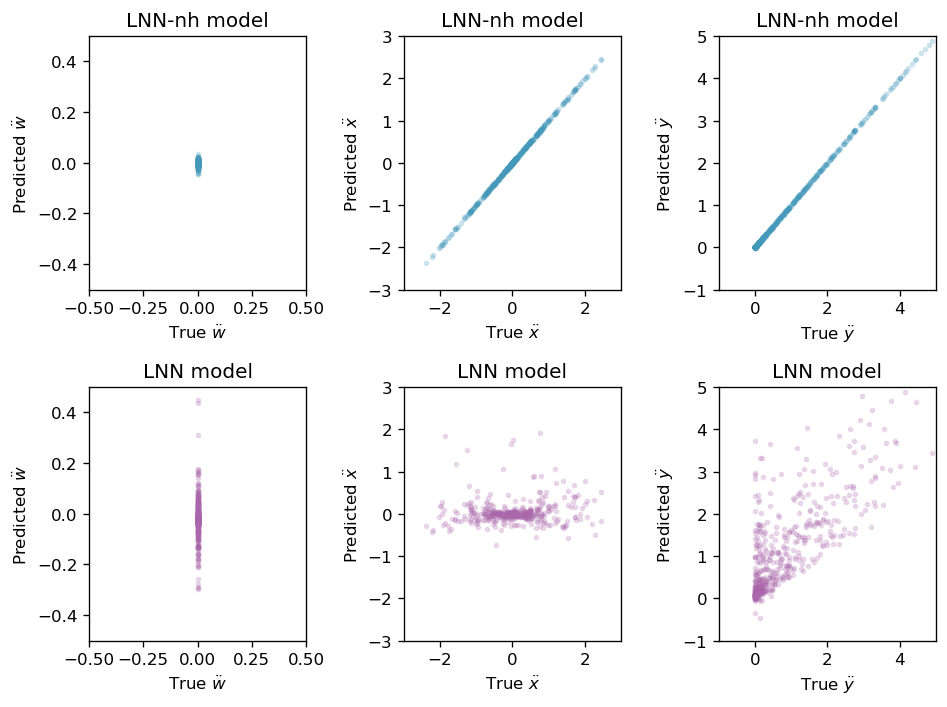
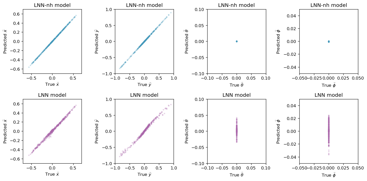
Figure 1 compares the learned and true value of each coordinate acceleration in the example for both models, exhibiting a major dispersion in LNN learned accelerations.
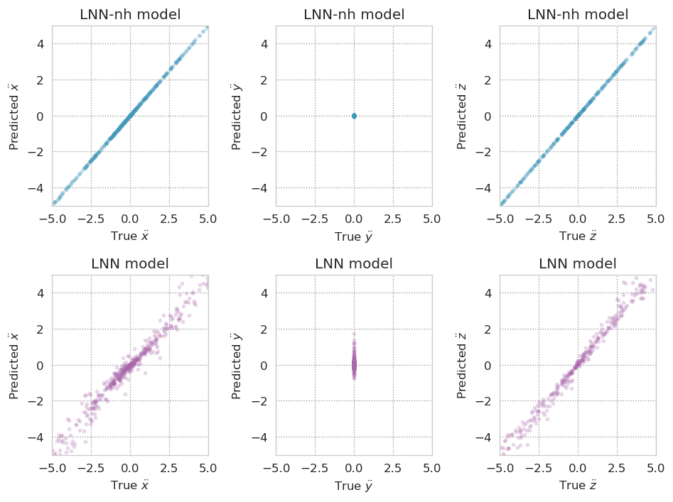
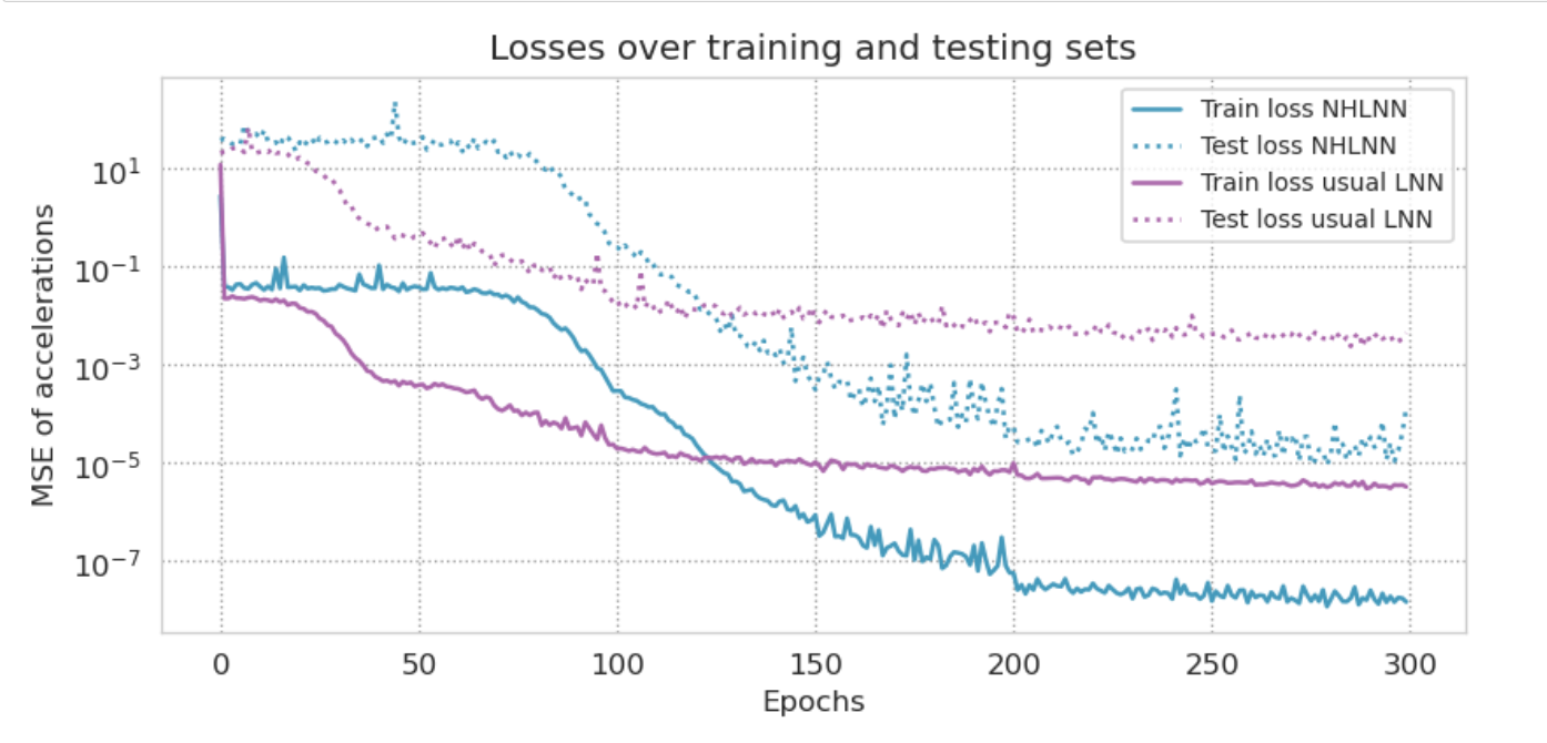
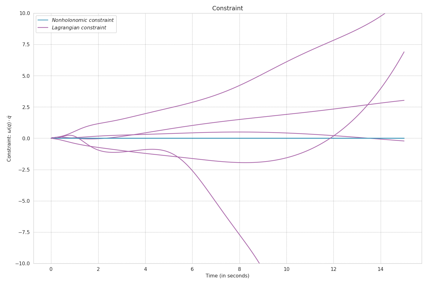
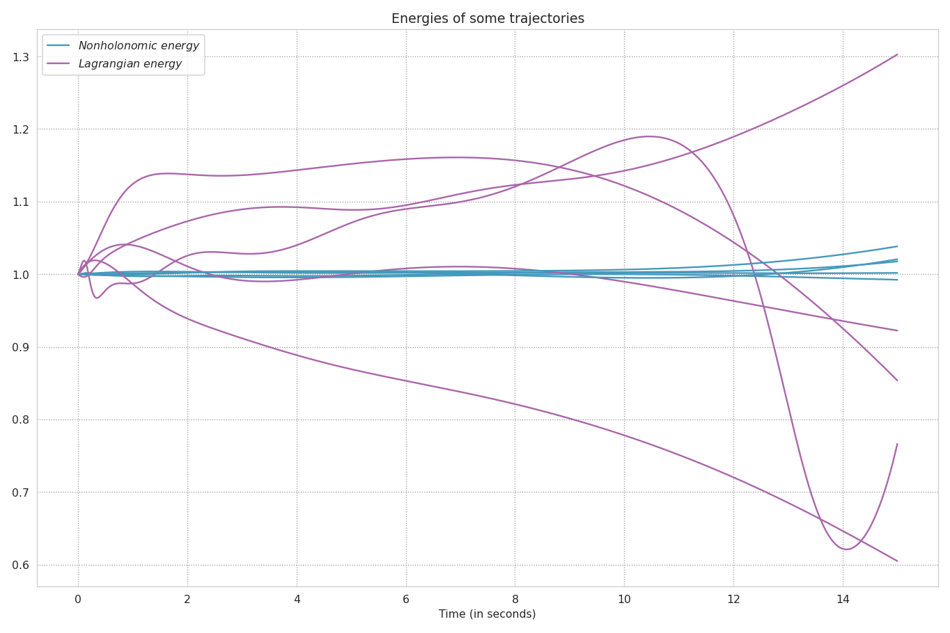
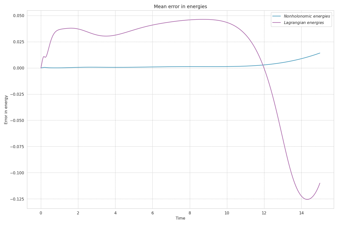
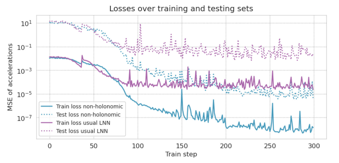
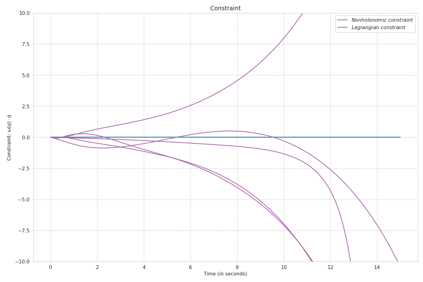
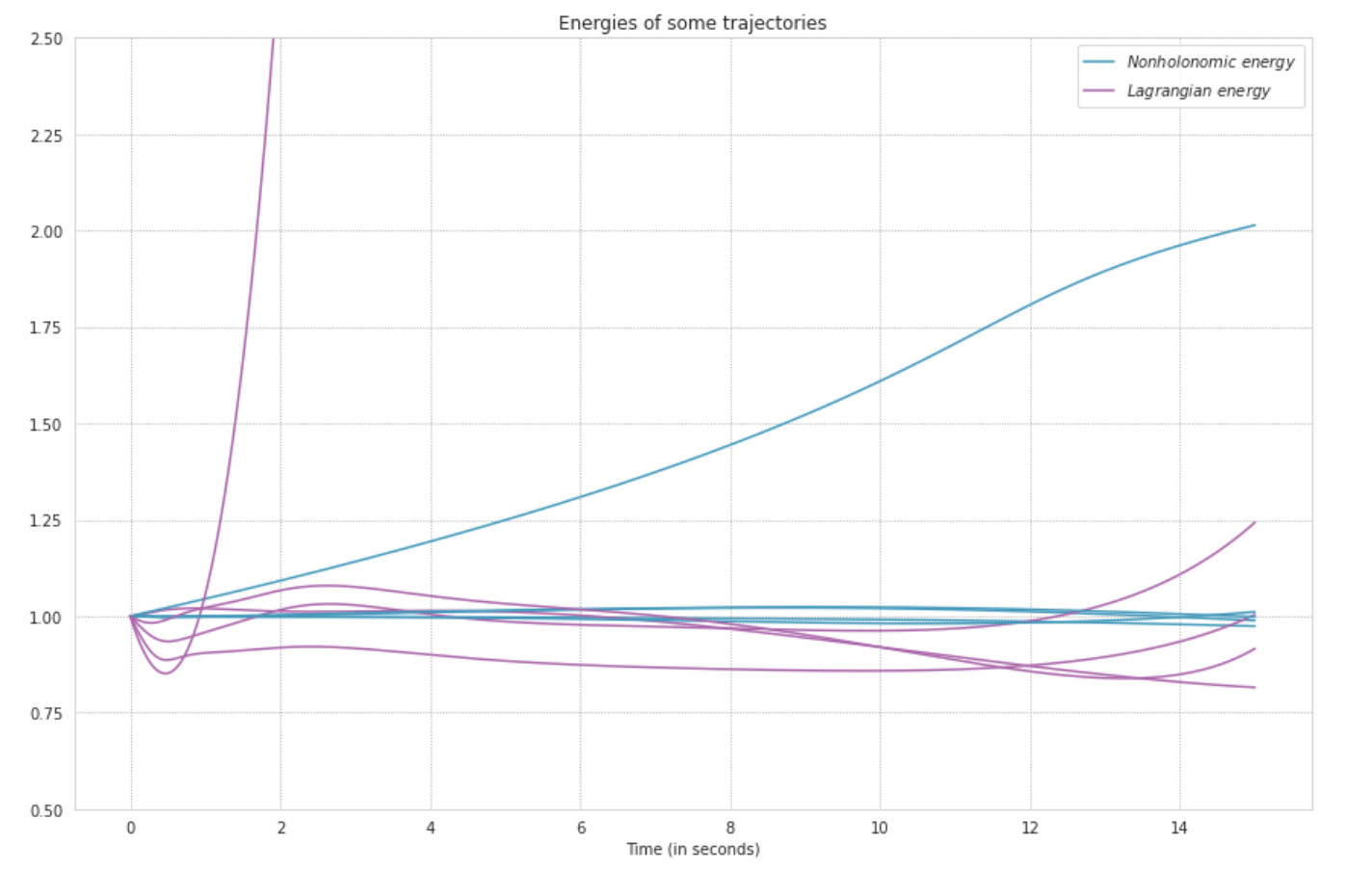
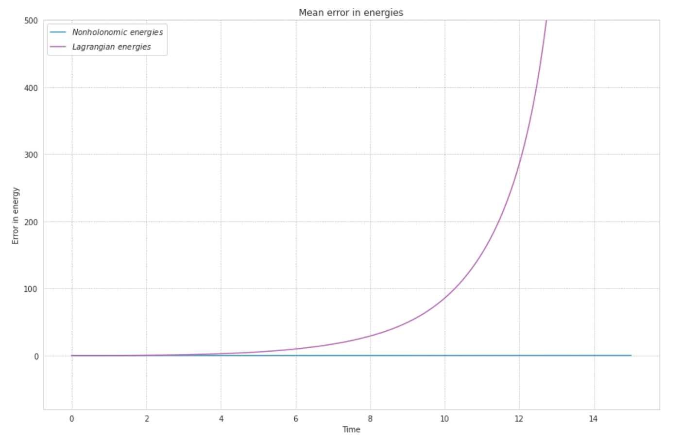
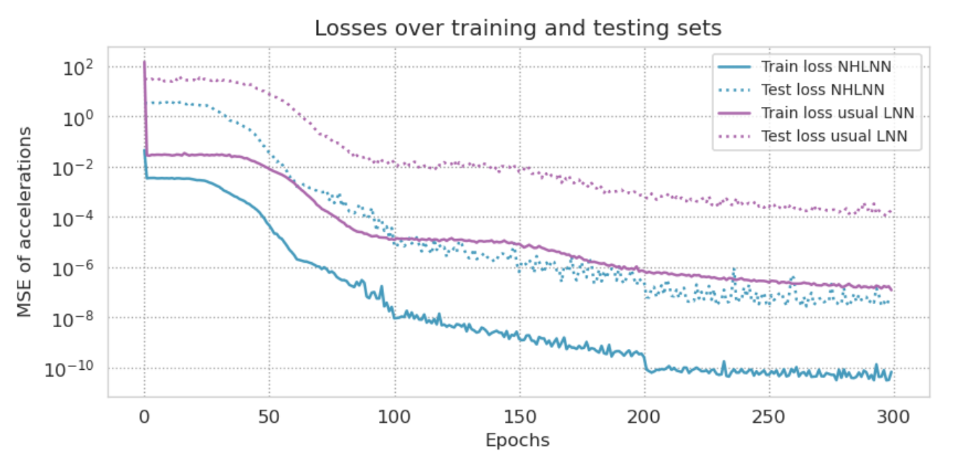
Figure 2 shows the comparison between the loss function in the case in which we learn the Lagrangian using a LNN and with a LNN-nh. Performance of energy and constraint functions over five learned trajectories of both models are also shown in the same picture.
6.2 Drone chasing a target
Consider a target and a drone moving in the plane. We take the target as a particle of mass moving freely along the axis and we take the drone as another particle of mass moving in the plane chasing the target, i.e. with velocity pointing directly to it (see [13] for details). The position of the target is determined with a single coordinate , whereas position of the drone may be described with two cartesian coordinates . Hence, the state of the system is completeley described by the tuple .
The Lagrangian of this system is given by
and the single constraint can be written as
Accordingly, , so we notice that the restriction is in fact linear, i.e. with . In this case, the matrix is the scalar and we have a unique Lagrange multiplier given by
Similar to the nonholonomic particle, we have no potential, so the force vanishes .
Gathering all this information, we can write the equations of motion as
Figure 3 shows the comparison between the learned and true value of each coordinate acceleration in the example for both models, exhibiting a major dispersion in LNN learned accelerations.
In Figure 4 we have included the results from models LNN and LNN-nh of the loss function, and the energy and constraint values for five different trajectories of the learned dynamics of the example. Computations are performed considering .
6.3 A vertical rolling wheel
A configuration of a wheel as a disk rolling without slipping in a vertical position in a plane is given by a point . The meaning of the variables is detailed, for instance, in [3, 1].
The Lagrangian is given by
where is the mass of the wheel and are the momenta of inertia. We consider , and in implementation. The rolling-without-slipping restriction is a constraint of rank two given by the equations
As in the previous examples, . On the other hand, we have
and
Consequently, Lagrange-d’Alembert equations give rise to following system
together with the constraint equations. In Figure 5 can be seen the comparison between the learned and true value of each coordinate acceleration for both models, exhibiting a major dispersion in LNN learned accelerations. Figure 6 in turn shows the evolution of loss functions over training for testing and training sets of the LNN and LNN-nh models. The same picture also shows the performance of the learned trajectories using both systems of the energy and constraint functions.
7 Conclusions
Regarding the loss graphs for training and testing for both models in the examples, we observe that although the initial values are nearly identical, the LNN-nh model shows a significantly steeper decrease in the loss function during training and testing. By the end of training, the LNN-nh model’s loss is two orders of magnitude lower than that of the LNN model. This difference in loss is evident in the greater deviation of the LNN model’s predicted accelerations from the actual values, as shown in the corresponding graphs for each example.
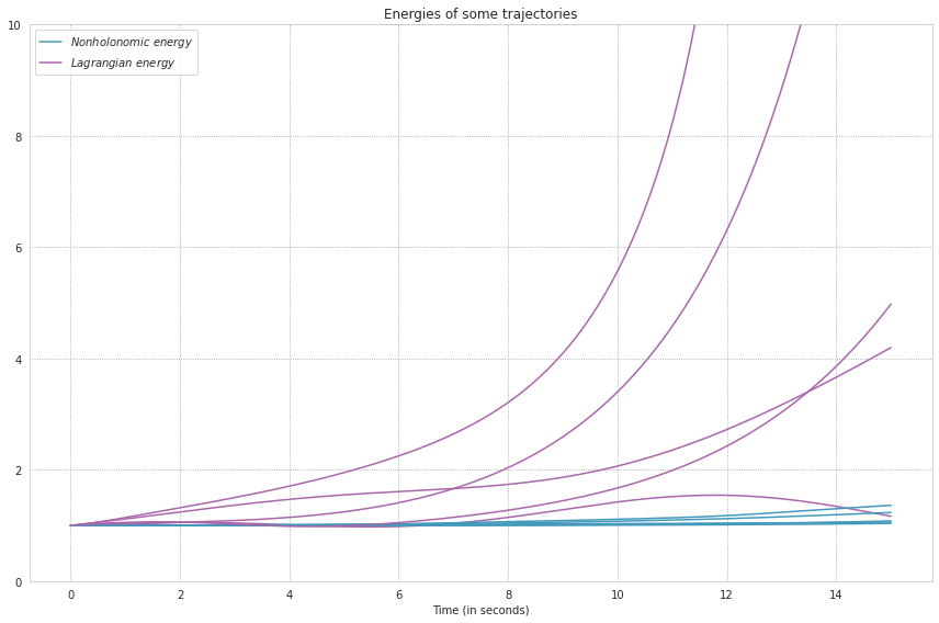
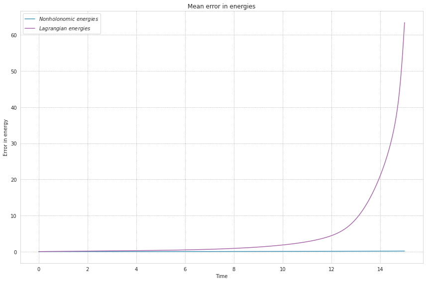
Concerning the conservation of energy, we can observe that the energy along LNN-nh-learned trajectories remains relatively stable over time, showing little to no increase in energy across various trajectories compared to the LNN counterpart, which exhibits fluctuations and a noticeable drift, even substantial divergence in some case, and an overall increase in energy over time. So, in general, the nonholonomic model demonstrates better stability and adherence to energy conservation principles.
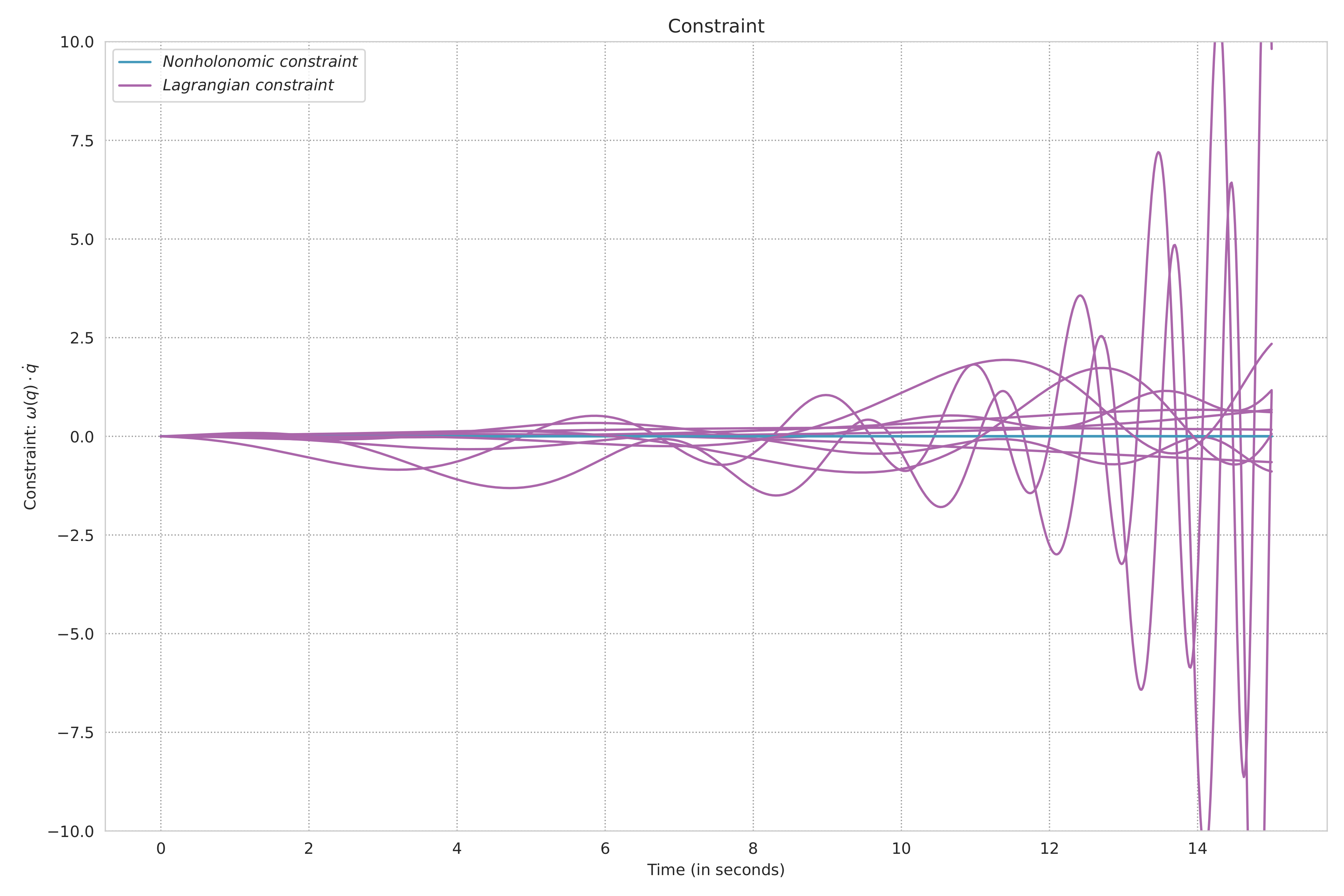
In terms of comparing the constraint’s behavior over time across the five trajectories of each example, the LNN model exhibits high variability, significant deviations, and sensitivity to changes over time, showing both positive and negative bias in some cases. In contrast, the LNN-nh estimation is consistently more stable, with minor fluctuations tending to remain close to zero and not showing significant differences.
The examples show that our model achieves significantly lower loss in both the training and test sets than the LNN model. It also consistently demonstrates effective energy stability and conservation, maintaining nearly constant energy levels along different trajectories. The implementations indicate that constraints from the LNN-nh model are more robust and stable over time than those from the LNN model, which are more susceptible to changes and rapidly drift away from the initial zero value of the constraint.
While the LNN model can be useful in certain contexts, it shows significant energy drift and instability in systems with nonholonomic constraints, making it less reliable for applications where energy conservation or preservation of the constraints is critical.
To summarize, across all experiments, the networks that incorporate the nonholonomic treatment of constraints into the loss function generally outperform the Lagrangian neural networks that do not consider the non-holonomic constraints. The results highlight the effectiveness of incorporating nonholonomic constraints in improving neural network performance for systems with such kind of restrictions.
References
- [1] J. Baillieul, A.M. Bloch, P. Crouch, and J. Marsden. Nonholonomic Mechanics and Control. Interdisciplinary Applied Mathematics. Springer New York, 2008.
- [2] E. Celledoni, M. Farré Puiggalí, E.H. Høiseth, and D. Martín de Diego. Energy-preserving integrators applied to nonholonomic systems. J. Nonlinear Sci., 29(4):1523–1562, 2019.
- [3] H. Cendra and V.A. Díaz. The Lagrange-d’Alembert-Poincaré Equations and Integrability for the Rolling Disk. Regular and Chaotic Dynamics, vol. 11(no. 1): pp. 67–81, 2006.
- [4] J. Cortés, M. de León, D. Martín de Diego, and S. Martínez. Geometric description of vakonomic and nonholonomic dynamics. comparison of solutions. SIAM J. Control. Optim., 41:1389–1412, 2000.
- [5] M. Cranmer, S. Greydanus, S. Hoyer, P. Battaglia, D. Spergel, and S. Ho. Lagrangian neural networks. In International Conference on Learning Representations, Workshop on Integration of Deep Neural Models and Differential Equations, 2020.
- [6] M. de Leon, J.C. Marrero, and D. Martin de Diego. Vakonomic mechanics versus non-holonomic mechanics: a unified geometrical approach. Journal of Geometry and Physics, 35(2):126–144, 2000.
- [7] M. Finzi, K.A. Wang, and A.G. Wilson. Simplifying Hamiltonian and Lagrangian neural networks via explicit constraints. In H. Larochelle, M. Ranzato, R. Hadsell, M.F. Balcan, and H. Lin, editors, Advances in Neural Information Processing Systems, volume 33, pages 13880–13889. Curran Associates Inc., 2020.
- [8] S. Greydanus, M. Dzamba, and J. Yosinski. Hamiltonian neural networks. In H. Wallach, H. Larochelle, A. Beygelzimer, F. d'Alché-Buc, E. Fox, and R. Garnett, editors, Advances in Neural Information Processing Systems, volume 32. Curran Associates, Inc., 2019.
- [9] S. LaValle. Planning algorithms. Cambridge University Press, 2006.
- [10] A.D. Lewis and R.M. Murray. Variational principles for constrained systems: Theory and experiment. International Journal of Non-Linear Mechanics, 30(6):793–815, 1995.
- [11] M. Lutter, C. Ritter, and J. Peters. Deep lagrangian networks: Using physics as model prior for deep learning. arXiv preprint arXiv:1907.04490, 2019.
- [12] M. Mattheakis, D. Sondak, A.S. Dogra, and P. Protopapas. Hamiltonian neural networks for solving equations of motion. Phys. Rev. E, 105:065305, Jun 2022.
- [13] M. Swaczyna. Several examples of nonholonomic mechanical systems. Communications in Mathematics, 19:27–56, 2011.
- [14] Peter Toth, Danilo Jimenez Rezende, Andrew Jaegle, Sébastien Racanière, Aleksandar Botev, and Irina Higgins. Hamiltonian generative networks. ArXiv, abs/1909.13789, 2019.
- [15] Y. D. Zhong, B. Dey, and A. Chakraborty. Benchmarking energy-conserving neural networks for learning dynamics from data. In Learning for dynmics and control, pages 1218–1229, 2021.