Baryon Pasting the Uchuu Lightcone Simulation

Abstract

We present the Baryon Pasted (BP) X-ray and thermal Sunyaev-Zel’dovich (tSZ) maps derived from the half-sky Uchuu Lightcone simulation. These BP-Uchuu maps are constructed using more than $75$ million dark matter halos with masses $M_{500c}\geq 10^{13}M_{\odot}$ within the redshift range $0\leq z\leq 2$. A distinctive feature of our BP-Uchuu Lightcone maps is their capability to assess the influence of both extrinsic and intrinsic scatter caused by triaxial gaseous halos and internal gas characteristics, respectively, at the map level. We show that triaxial gas drives substantial scatter in X-ray luminosities of clusters and groups, accounting for nearly half of the total scatter in core-excised measurements. Additionally, scatter in the thermal pressure and gas density profiles of halos enhances the X-ray and SZ power spectra, leading to biases in cosmological parameter estimates. These findings are statistically robust due to the extensive sky coverage and large halo sample in the BP-Uchuu maps. The BP-Uchuu maps are publicly available online via Globus.

1 Introduction

Ongoing and upcoming large-scale multiwavelength sky surveys in X-ray, microwave, and optical of galaxy clusters are promising for improving our understanding of cosmology. This is going to be achieved with significant reduction of statistical uncertainties owing to the large cosmological volumes that these surveys will probe. In particular, the order of magnitude increase in the number of galaxy clusters and groups compared to cluster surveys in the previous decade will dramatically improve the cosmological constraints of cluster abundance measurements (see Allen et al., 2011, for a review). The extensive sky coverage of these surveys also enables cross-correlations of clusters and groups as powerful cosmological and astrophysical probes (e.g., Shirasaki et al., 2020). The success of these surveys depends on our ability to accurately model and mitigate systematic uncertainties, which can profoundly influence the distribution and evolution of matter on small to intermediate scales.

Accurate estimation of the mass-observable scaling relations is fundamental to derive reliable constraints on key cosmological parameters in cluster abundance cosmology (Pratt et al., 2019). These scaling relations connect the halo mass to observable properties, such as X-ray luminosity or the thermal Sunyaev–Zeldovich (tSZ) signal at microwave wavelengths, enabling indirect mass estimation in cosmological surveys (e.g., Vikhlinin et al., 2009; Mantz et al., 2010; Benson et al., 2013; Bocquet et al., 2019). However, these relations often fail to capture the full complexity of physical systems because they do not account for the scatter around the mean relations (e.g., Mantz et al., 2016; Sereno et al., 2020). While scatter provides direct information on the structure and evolution of these systems (Farahi et al., 2019), failing to account for scatter biases in the interpretation of observational data (Farahi et al., 2019; Costanzi et al., 2019; Zhang et al., 2024), thereby affecting the precision estimates of crucial cosmological parameters such as the matter density ($\Omega_{m}$) and the amplitude of matter fluctuations ($\sigma_{8}$).

Scatter in scaling relations can be categorized into two primary sources: intrinsic and extrinsic. Intrinsic scatter arises from internal physical processes within the halo, such as baryonic physics such as feedback from supernovae (SNe) and active galactic nuclei (AGN), radiative gas cooling, and star formation, all of which influence the thermodynamics of the halo gas (e.g., Farahi et al., 2018; Truong et al., 2018; Pop et al., 2022; Yang et al., 2022). Extrinsic scatter, on the other hand, originates from external factors such as the non-spherical (triaxial) nature of halos and projection effects. Similarly to dark matter (DM) distributions, the gas distributions in clusters and groups are typically triaxial (Lau et al., 2011; Mulroy et al., 2019; Kim et al., 2024), and the observed signals can be affected by the orientation of the halo’s major axis relative to the line of sight (e.g., Limousin et al., 2013). Understanding and quantifying both intrinsic and extrinsic scatter is essential to improve the accuracy of mass estimates and minimizing biases in cosmological inferences.

To date, extrinsic scatter in cosmological inferences remains incompletely quantified. Current simulations often lack the resolution or comprehensive physical models necessary to accurately capture the interplay between various baryonic processes that contribute to correlated and extrinsic scatter. They are also expensive to run, making them less suitable for exploring the wide parameter spaces required for upcoming large-scale multiwavelength surveys, where numerous combinations of cosmological and astrophysical parameters must be tested (Mead et al., 2021; Villaescusa-Navarro et al., 2021; Schaye et al., 2023). However, observational constraints on these types of scatter are limited as it is difficult to separate extrinsic scatter from intrinsic scatter with observations. This makes it challenging for observations to validate and refine simulation predictions of intrinsic scatter. The inability to efficiently explore these parameter spaces hampers our capacity to fully understand and mitigate the systematic uncertainties introduced by baryonic physics in cosmological analyses.

A complementary and more feasible approach involves the use of empirical and analytic methods to model baryonic properties within DM halos (see Wechsler & Tinker, 2018, for a review). This strategy entails forward-modeling baryonic properties by overlaying them onto DM halos from relatively inexpensive large-scale DM-only cosmological simulations. These baryon-DM models are calibrated using either detailed cosmological simulations or high-quality observational datasets. By varying the underlying baryon-DM models and cosmological parameters within DM-only simulations, one can efficiently study the dependence of baryonic effects on astrophysical processes and cosmology. This empirical and analytic framework not only facilitates the exploration of a broader parameter space but also supports the statistical inference necessary to maximize the scientific return of upcoming surveys. Moreover, it allows for rapid iterations and refinements based on new observational data, ensuring that the models remain accurate and relevant in the rapidly evolving landscape of cosmological research.

Although significant efforts have been dedicated to painting galaxy properties onto DM halos (e.g., Seljak, 2000; Moster et al., 2018; Behroozi et al., 2019; Hadzhiyska et al., 2020), fewer works focus on painting gas properties. Existing gas painting techniques in the literature (Valotti et al., 2018; Clerc et al., 2018; Zandanel et al., 2018; Stein et al., 2020; Comparat et al., 2020; Omori, 2022; Williams et al., 2023; Bayer et al., 2024) rely on phenomenological or empirical gas models calibrated with cosmological hydrodynamical simulations or observations. One key disadvantage of this approach is that empirical parameters often lack direct physical interpretation, making them less useful for interpreting observations or for understanding the underlying physics.

Alternatively, advances in machine learning techniques have been applied to paint galaxies or gas on DM halos (e.g., Agarwal et al., 2018; Chadayammuri et al., 2023; Nguyen et al., 2024). However, these approaches are often “black boxes”, making them difficult to interpret physically. Hybrid approaches (e.g., Kéruzoré et al., 2024), calibrate parameters of gas analytical models using machine learning, offering more physically interpretable models. Nevertheless, they still rely on large training samples of input simulations that are expensive to produce and are subject to the same subgrid physics uncertainties inherent in the simulations they are trained on.

To address the challenges of modeling halo gas for large-scale multiwavelength galaxy surveys, we have developed Baryon Pasting (BP), a code specifically designed to paint gas onto DM halos efficiently and fast, with physically motivated models. BP provides physically interpretable modeling of gas in DM halos, which is essential for astrophysical and cosmological inferences from observations. It enables rapid exploration of how feedback physics and non-thermal pressure support affect the tSZ power spectrum (Shaw et al., 2010), how cool-dense cores affect optical depth measurements of clusters and groups in kinetic SZ observations (Flender et al., 2017), and how to break the degeneracies between astrophysical and cosmological parameters in cross-correlations of X-ray, tSZ, and lensing measurements of galaxy clusters and groups (Shirasaki et al., 2020). Painting gas on DM particles in the simulation allows us to model gas observables in cosmic web filaments (Osato & Nagai, 2023). Unlike purely empirical or machine learning-based methods, BP maintains physical interpretability while remaining computationally efficient, making it well-suited for the extensive parameter space exploration required by upcoming surveys.

In this paper, we present the updated BP gas model and apply it to create half-sky multi-wavelength maps using the DM-only Uchuu Lightcone simulations (Ishiyama et al., 2021). Specifically, these BP-Uchuu mock maps enable quantification of the impact of halo triaxiality on the X-ray luminosity ($L_{X}$)–mass scaling relation, focusing specifically on extrinsic scatter. We classify scatter due to triaxiality and projection as extrinsic, differentiating it from intrinsic scatter caused by internal halo processes. Our results show that halo orientation plays a significant role in modulating observed X-ray luminosity, with halos aligned along the line of sight exhibiting enhanced luminosities. Specifically, halos with their elongated axis more aligned with the line-of-sight direction tend to show systematically higher $L_{X}$ values for a given mass. The comparison between triaxial and spherical halos reveals that this bias is not merely a projection effect, but rather a result of halo shape and orientation, contributing an additional scatter to the $L_{X}$ measurements. This extrinsic scatter is non-negligible at the $8\%-9\%$ level, at around 1/3 and 1/2 of the total scatter, for non-core-excised and core-excised $L_{X}$, respectively. Our results further highlight the importance of accounting for halo triaxiality in precision cosmological analyses. In addition, we also show that the scatter in the halo gas profiles leads to $\sim 10\%-40\%$ biases in the X-ray and tSZ angular power spectra of clusters and groups (Hurier et al., 2015; Planck Collaboration et al., 2016; Lau et al., 2023, 2024). Interpretation of the power spectrum that uses the halo model usually does not include intrinsic scatter in halo gas profiles, leading to underestimates of the actual amplitude of the power spectrum and thus biases the derived constraints on cosmological parameters such as $\sigma_{8}$ and $\Omega_{m}$.

We give an overview of the BP gas model in Section 2 and how the BP maps are generated in Section 3. We present results with the Uchuu BP maps in Section 4. Finally, we give our conclusions in Section 6.

2 Gas Model

Parameter	Physical meaning	Equation	Default Value
$\epsilon_{f}$	feedback efficiency from SNe and AGN	Eq. (7)	$3.97\times 10^{-6}$
$\epsilon_{\rm DM}$	DM energy transfer to gas	Eq. (7)	$0.0$
$f_{\star}$	amplitude of the stellar mass fraction	Eq. (8)	$0.026$
$S_{\star}$	mass slope of stellar mass fraction	Eq. (8)	$0.12$
$x_{\mathrm{break}}$	cluster core radius in $R_{500}$	Eq. (6)	$0.195$
$\Gamma$	polytropic index outside the cluster core	Eq. (6)	$1.2$
$\Gamma_{0}$	polytropic index within cluster core	Eq. (6)	$0.1024$
$\beta_{g}$	redshift evolution of polytropic index within cluster core	Eq. (6)	$1.72$
$A_{\rm nt}$	amplitude of non-thermal pressure fraction profile	Eq. (11)	0.452
$B_{\rm nt}$	scale of the radial dependence of the non-thermal pressure fraction profile in $R_{200m}$	Eq. (11)	0.841
$\gamma_{\rm nt}$	logarithmic slope of non-thermal pressure fraction profile	Eq. (11)	1.628
$R_{\rm bound}$	Boundary of the gas in halo in DM splashback radius $R_{\rm sp}$	–	1.89

Table 1: Default values of the Gas model parameters adopted by our BP gas model. They are taken from the best fits of the gas density profiles from Chandra-SPT cluster samples from Flender et al. (2017), except the parameters for the non-thermal pressure fraction profile and the clumping profile, which are taken from the fit to the Omega500 cosmological simulation (Nelson et al., 2014b).

Figure 1: A Schematic diagram showing the general structure of BP map-making. We start with an input halo catalog with information on the redshift, mass (specifically $M_{\rm vir}$), and positions (RA and Dec) of the halo. Given the halo mass and redshift, we generate the gas profiles (X-ray emissivity, Compton-$y$) using the BP gas model. The profiles are then painted onto the X-ray Surface Brightness (XSB) and thermal Sunyaev-Zeldovich (tSZ) maps using the position information.

Figure 1 illustrates the general structure of how BP maps are generated from halo catalogs. We take 4 main halo information: redshift, mass (specifically virial mass), right ascension (RA) and declination (Dec) from the halo catalog. Optionally, we also take the halo shape information: axis ratios and the angle between the major axis and the line-of-sight for generating maps with triaxial halos. The redshift and virial mass then serve as inputs to the BP gas model to generate gas profiles in density, pressure, temperature, Compton-$y$ profile, and X-ray emissivity profile for each halo. The gas profiles also serve as one of the primary data products from which other observables, such as scaling relations and power spectra, are derived. To generate the map, for each halo we paint the profile (Compton-$y$ profile or the X-ray emissivity profile) at the corresponding RA and Dec of the halo on the map.

2.1 Halo Gas Profiles

Here we briefly review the salient features of the core BP gas model, which are described in detail in Shaw et al. (2010); Flender et al. (2017); Osato & Nagai (2023). The basic assumption of the BP model is that the DM halo follows the profile Navarro–Frenk–White (NFW) profile (Navarro et al., 1996),

$$\rho_{\mathrm{NFW}}(r)=\frac{\rho_{s}}{(r/r_{s})(1+r/r_{s})^{2}}$$ (1)

where $r_{s}$ is the NFW scale radius and $\rho_{s}$ is the normalization, which is completely specified by the virial mass of the halo $M_{\rm vir}$ and the halo concentration parameter $c_{\rm vir}$, which is defined as the ratio of the virial radius $R_{\mathrm{vir}}$ to the scale radius $r_{s}$ where the logarithmic slope of the DM density is $-2$. The virial radius is the radius of the sphere enclosing the virial mass, $M_{\mathrm{vir}}=\frac{4}{3}\pi R_{\mathrm{vir}}^{3}\Delta_{\mathrm{vir}}\rho_{c}(z)$ with $\Delta_{\mathrm{vir}}=18\pi^{2}+82(\Omega_{M}(z)-1)-39(\Omega_{M}(z)-1)^{2}$ (Bryan & Norman, 1998), and $\rho_{c}(z)$ is the critical density at redshift $z$.

The BP gas model assumes the total gas pressure (thermal + non-thermal) $P_{\rm{tot}}$ is in hydrostatic equilibrium (HSE) with the gravitational potential of the halo, and that the relationship between $P_{\rm{tot}}$ and the gas density $\rho_{g}$ is related through the polytropic relation,

$$P_{\rm{tot}}(r) = P_{0}\theta(r)^{n+1},$$ (2)

$$\rho_{g}(r) = \rho_{0}\theta(r)^{n},$$ (3)

$$\theta(r) = 1+\frac{\Gamma-1}{\Gamma}\frac{\rho_{0}}{P_{0}}(\Phi(r=0)-\Phi(r)),$$ (4)

where $\theta$ is a dimensionless function that represents the gas temperature, $\Phi$ is the gravitational potential of the halo given by the NFW profile,

$$\Phi_{\rm NFW}=-\frac{4\pi G\rho_{s}r_{s}^{3}}{r}\ln\left(1+\frac{r}{r_{s}}\right),$$ (5)

and ${\Gamma=1+1/n}=1.2$ and $n=5$ are the polytropic exponent and the polytropic index respectively, whose values are set to match those in cosmological hydrodynamical simulations (Komatsu & Seljak, 2001; Ostriker et al., 2005; Shaw et al., 2010; Battaglia et al., 2012). The values are also consistent with recent observations of the polytropic index (Ghirardini et al., 2019).

Following Flender et al. (2017), we model the gas in the cores of halos differently with different polytropic equations of state than the rest of the halo. Due to strong cooling and feedback in the core, the gas in the core is denser and colder, thus we adopt a smaller polytropic exponent than the outer region:

$$\Gamma=\begin{cases}1.2&r_{\rm break}/R_{500c}\geq x_{\rm break},\\ \Gamma_{0}(1+z)^{\beta}&r_{\rm break}/R_{500c}<x_{\rm break},\end{cases}$$ (6)

with $x_{\rm break}=r_{\rm break}/R_{500c}$ representing the radial extent of the halo core in units of $R_{500c}$ of the halo. Following Flender et al. (2017), we set $\Gamma_{0}=0.1024$, $\beta_{g}=1.72$, and $x_{\rm break}=0.195$.

The normalization constants $P_{0}$ and $\rho_{0}$ are determined numerically by solving the energy and momentum conservation equations of the gas. In particular, the energy of the gas is given by

$$E_{g,f}=E_{g,i}+\epsilon_{\rm DM}|E_{\rm DM}|+\epsilon_{f}M_{\star}c^{2}+\Delta E_{p}.$$ (7)

where $E_{g,f}$ and $E_{g,i}$ are the final and initial total energies (kinetic plus thermal plus potential) of the ICM. $\Delta E_{p}$ is the work done by the ICM as it expands. $\epsilon_{\rm DM}|E_{\rm DM}|$ is the energy transferred to the ICM during major halo mergers via dynamical friction. Note that the exact value of $\epsilon_{\rm DM}$ remains highly uncertain and depends on other factors such as the merger history of a given halo. We use the outer accretion shock as the boundary of the gas, which is approximately $1.89$ times the splashback radius $R_{\rm sp}$ informed by results from cosmological simulations (Aung et al., 2021). For the value of $R_{\rm sp}$, we use the fitting function from Equation (7) in More et al. (2015) which relates $R_{\rm sp}$ with the halo peak height $\nu_{200m}\equiv 1.686/\sigma(M_{200m},z)$, where $\sigma(M,z)$ is the variance of density fluctuations at the redshift $z$ on the mass scale $M$. This sets the boundary condition for solving the momentum conservation equation.

The term $\epsilon_{f}M_{\star}c^{2}$ represents the energy injected into the ICM due to feedback from both supernovae (SNe) and active galactic nuclei (AGN), where $M_{\star}$ is the total stellar mass. The stellar mass is given by the stellar fraction $F_{\star}(<R_{500c})=M_{\star}(<R_{500c})/M_{500c}$, which depends only on the halo mass as

$$F_{\star}(M_{500c})=f_{\star}\left(\frac{M_{500c}}{3\times 10^{14}M_{\odot}}\right)^{-S_{\star}}.$$ (8)

which is described by two parameters $(f_{\star},S_{\star})$ that control the normalization and the slope of the $F_{\star}-M$ relation. Following (Flender et al., 2017), we choose $f_{\star}=0.026$ and $S_{\star}=0.12$ as our fiducial parameters. These values are chosen to match the values of the observed stellar mass fraction (see Table 2 in Flender et al., 2017).

Alternatively, the gas mass fraction can be set instead of the stellar mass fraction:

$$F_{\rm gas}(M_{500c})=f_{\rm gas}\left(\frac{M_{500c}}{3\times 10^{14}M_{\odot}}\right)^{S_{\rm gas}}.$$ (9)

where the two free parameters are $(f_{\rm gas},S_{\rm gas})$. The sum of the gas mass fraction and stellar mass fraction is assumed to be equal to the cosmic baryon fraction $f_{b}=\Omega_{b}/\Omega_{M}$, independent of halo mass and redshift:

$$F_{\rm gas}(M_{500c})+F_{\star}(M_{500c})=f_{b}.$$ (10)

We use a radially-dependent non-thermal pressure from Nelson et al. (2014a):

$$f_{\rm nt}\equiv\frac{P_{\rm rand}(r)}{P_{\rm tot}(r)}=1-A_{\rm nt}\left[1+\exp\left\{-\left(\frac{r}{B_{\rm nt}\,R_{200m}}\right)^{C_{\rm nt}}\right\}\right],$$ (11)

where $R_{\rm 200m}$ is the spherical over-density radius with respect to 200 times the mean matter density of the universe. The parameters are calibrated to be $A_{\rm nt}=0.452$, $B_{\rm nt}=0.841$, $C_{\rm nt}=1.628$. The $R_{\rm 200m}$ scaling ensures halo redshift and mass independence at the cluster scales $M_{500c}\geq 3\times 10^{14}h^{-1}M_{\odot}$ over which this relation is calibrated with the Omega500 cosmological simulation (Nelson et al., 2014a). The thermal pressure $P_{\rm th}$ is obtained by multiplying $P_{\rm tot}$ with $(1-f_{\rm nt})$.

Table 1 summarizes the parameters of the BP gas model, their physical meanings, and default values.

2.2 Calculating X-ray and thermal SZ Observables

We compute the X-ray emissivity profile of a given halo as

$$\epsilon_{X}(r;M_{\rm vir},z) =\frac{n_{H}(r;M_{\rm vir},z)n_{e}(r;M_{\rm vir},z)}{4\pi(1+z)^{4}}$$ (12)

$$\times\int^{E_{\rm max}(1+z)}_{E_{\rm min}(1+z)}\Lambda(T(r;M_{\rm vir},z),Z,E)dE$$

where $n_{H}$, $n_{e}$ and $T$ are the hydrogen and electron number densities and gas temperature respectively. We use the APEC plasma code version 3.0.9 (Foster et al., 2012) to compute the X-ray cooling function $\Lambda$, integrated over the energy range $[E_{\rm min},E_{\rm max}]$ in the observer’s frame. The fiducial values for $E_{\rm min}$ and $E_{\rm max}$ are $0.5$ and $2.0$ keV respectively. We assumed a constant metallicity of $Z=0.3Z_{\odot}$ throughout the ICM, as suggested from observations (e.g., Mernier et al., 2018), and we used the Solar abundance values from Asplund et al. (2009).

The Compton-$y$ profile of a given halo is directly derived from the thermal pressure profile:

$$y(r;M_{\rm vir},z)=\frac{\sigma_{T}}{m_{e}c^{2}}\frac{\mu}{\mu_{e}}P_{\rm th}(r;M_{\rm vir},z),$$ (13)

where $\sigma_{T}=6.25\times 10^{-25}\,{\rm cm^{2}}$ is the Thomson cross-section, $m_{e}c^{2}=511\,{\rm keV}$ is the electron rest mass energy, and $P_{\rm th}(r;M_{\rm vir},z)$ is the thermal gas pressure profile. Here $\mu=4/(5X+3)$ and $\mu_{e}=2/(X+1)$ are the mean molecular weights of the fully ionized gas and electron, respectively, with $X=0.76$ the primordial hydrogen mass fraction.

2.3 Triaxial Gas Halo and its 2D Projection

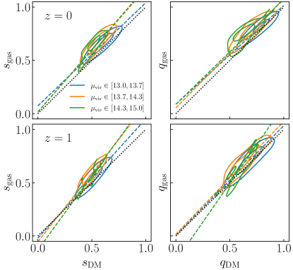
Figure 2: Plots of gas shape versus DM shape in halos in different mass bins with $\mu_{\rm vir}\equiv\log_{10}(M_{\rm vir}/M_{\odot})$ from the TNG300 simulations at $z=0$ (upper panels) and $z=1$ (lower panels). The solid lines indicate the $1,2,3\sigma$ of the density distributions of the number of halos. The dashed lines are the bisector fits to the relation between gas and DM shape. The left panel shows the short-to-long axis ratio $s=c/a$, and the right panel shows the mid-to-long axis ratio $q=b/a$, where $a\geq b\geq c$ being the major, middle, and minor axes of the triaxial ellipsoid, respectively. The black dotted lines show where $s_{\rm gas}=s_{\rm DM}$ and $q_{\rm gas}=q_{\rm DM}$.

DM and gas in halos are triaxial instead of spherical, as shown in both observations and cosmological simulations. Halo triaxiality is a natural consequence of cold DM structure formation. It is expected that halo triaxiality leads to bias and scatter in observable-mass scaling relations and bias in cluster selection functions. However, in most analytical models or observational analyses, both the DM and gas halos are treated as spherical halos.

In BP, we model the triaxial shapes of both DM and gas halos to investigate their impact on cluster observables. The BP code uses the provided axis ratios from the DM halo catalog.

Cosmological simulations show that gas halos are more spherical than their DM hosts. To model the gas shape, we calibrate an empirical model of the dependence of the gas shape on the DM shape using the shape measurements from the IllustrisTNG300 cosmological hydrodynamical simulations.

The gas axis ratios for the given DM axis ratios with masses between $\log_{10}(M_{\rm vir}/M_{\odot})=[13.0,15.0]$ for $0\leq z\leq 2$ are expressed as

$$s_{\rm gas} = s_{0}+s_{1}s_{\rm DM},$$ (14)

$$q_{\rm gas} = q_{0}+q_{1}q_{\rm DM}.$$ (15)

We model their mass and redshift dependence with

$$s_{0} = 1.78-1.82\mu_{14}+0.185\zeta,$$ (16)

$$s_{1} = -3.41-4.66\mu_{14}+0.281\zeta,$$ (17)

$$q_{0} = 0.73-0.687\mu_{14}-0.204\zeta,$$ (18)

$$q_{1} = -0.45+149\mu_{14}+0.204\zeta,$$ (19)

where $\mu_{14}\equiv\log_{10}(M_{\rm vir}/10^{14}M_{\odot})$ and $\zeta\equiv\log_{10}(1+z)$. Note that these relations are calibrated on the TNG300 simulations. In principle, they depend on the underlying baryon physics (Kazantzidis et al., 2004), which varies between different simulations.

We extend the analytical procedure to transform a spherically symmetric radial profile into a triaxial one by extending the formalism from Stark (1977). Denoting $(x,y,z)$ and $(x^{\prime},y^{\prime},z^{\prime})$ as the coordinate frames of the triaxial halo and the observers respectively, where $z^{\prime}$ aligns with the line-of-sight (LOS) direction, the two reference frames are related by the transformation $(x,y,z)^{T}=\mathbf{A}(x^{\prime},y^{\prime},z^{\prime})^{T}$ where

$$\mathbf{A}=\begin{pmatrix}c_{1}c_{3}-s_{1}c_{2}s_{3}&-c_{1}s_{3}-s_{1}c_{2}c_{3}&s_{1}s_{2}&\\ s_{1}c_{3}+c_{1}c_{2}s_{3}&-s_{1}s_{3}+c_{1}c_{2}c_{3}&-c_{1}s_{2}\\ s_{2}s_{3}&s_{2}c_{3}&c_{2}\end{pmatrix}.$$ (20)

Here we adopt a short-hand notation for $\cos$ and $\sin$ as $c$ and $s$ respectively, and $(1,2,3)$ stands for the Euler angles $(\phi,\theta,\psi)$ that specify the rotation. Specifically, $\theta$ is the angle between the major axis with the line-of-sight axis $z^{\prime}$, with $\theta\in[0,\pi/2]$, while $\phi\in[0,2\pi)$ and $\psi\in[0,2\pi)$.

For any generic 3D spherical profile $f_{3D}(r)$, we can substitute the spherical radius $r$ with the ellipsoidal radius $r_{\rm ep}$, where the triaxial profile is then described by $f_{3D}(r_{\rm ep})$. The ellipsoidal radius in the observer’s frame (the primed frame) is defined as

$$r_{\rm ep}^{2}=fz^{\prime 2}+gz^{\prime}+h,$$ (21)

where

$$f =A_{13}^{2}/s^{2}+A_{23}^{2}/q^{2}+A_{33}^{2},$$ (22)

$$g =2\left(A_{11}A_{13}/(s^{2})+A_{21}A_{23}/(q^{2})+A_{31}A_{33}\right)x^{\prime}$$ (23)

$$+2\left(A_{12}A_{13}/(s^{2})+A_{22}A_{23}/(q^{2})+A_{32}A_{33}\right)y^{\prime},$$

$$h =\left(A_{11}^{2}x^{\prime 2}+A_{12}^{2}y^{\prime 2}+2A_{11}A_{12}x^{\prime}y^{\prime}\right)/s^{2}$$ (24)

$$+\left(A_{21}^{2}x^{\prime 2}+A_{22}^{2}y^{\prime 2}+2A_{21}A_{22}x^{\prime}y^{\prime}\right)/q^{2}$$

$$+\left(A_{31}^{2}x^{\prime 2}+A_{32}^{2}y^{\prime 2}+2A_{31}A_{32}x^{\prime}y^{\prime}\right),$$

where $A_{ij}$ are the entries of the rotational matrix $\mathbf{A}$ in Equation (20), $q=b/a$, $s=c/a$ are the axis ratios, with $a\geq b\geq c$ being the major, middle, and minor axes of the triaxial ellipsoid respectively.

We then project the 3D triaxial profile $f_{3D}(r_{\rm ep})$ to the 2D distribution given by

$$F_{2D}(x^{\prime},y^{\prime}) \equiv\int_{-r_{\rm max}}^{r_{\rm max}}f_{3D}(r_{\rm ep})dz^{\prime}$$ (25)

$$=2\sqrt{f}\int_{0}^{r_{\rm max}}f_{3D}(\sqrt{z_{\star}^{2}+\zeta^{2}})dz^{\prime},$$

where $z_{\star}=\sqrt{f}\left(z^{\prime}+g/(2f)\right)$, $\zeta=h-{g^{2}}/{(4f)}$, and we set $r_{\rm max}=\sqrt{f}\left(5R_{500c}+g/(2f)\right)$.

2.4 Modeling intrinsic scatter in halo gas profiles

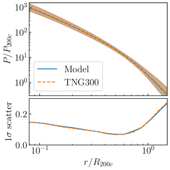
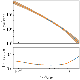
Figure 3: Top and bottom panels show the model pressure and density profiles sampled from the covariance matrix computed from the TNG300 simulation (solid blue), compared to the input TNG300 profiles (dashed orange). The lines and the shaded regions are the mean profiles $1\sigma$ scatter (over the natural logarithm of the profiles). The bottom subpanels in both panels show the $1\sigma$ scatter for the sampled and input TNG profiles.

BP map-making also includes a method of incorporating variations in the gas profiles due to differences in their formation histories and baryonic physics. Specifically, we adopt a non-parametric, empirical approach using the covariance of gas profiles measured from empirical data or cosmological simulations, following Comparat et al. (2020).

In the model presented here, we use the IllustrisTNG300 simulations to compute the covariance matrices for the logarithm of the thermal pressure and gas density. Specifically, for a generic profile $f(r)$ for each mass and redshift bin, we measure the covariance matrix $\mathcal{C}(r,r^{\prime})$ as

$$\mathcal{C}(r,r^{\prime})=\langle(\ln f(r)-\overline{\ln f}(r))(\ln f(r^{\prime})-\overline{\ln f}(r^{\prime}))\rangle$$ (26)

summing over all halos in the bin, where $\overline{\ln f}(r)$ is the mean profile in natural logarithm at radius $r$. We normalize the gas profiles with respect to their self-similar quantities:

$$P_{200c} = \frac{GM_{200c}}{2R_{200c}}200\rho_{\rm crit}(z)f_{b},$$ (27)

$$\rho_{200c} = 200\times\rho_{\rm crit}(z),$$ (28)

where $f_{b}=\Omega_{b}/\Omega_{M}$ is the cosmic baryon fraction, and $\rho_{\rm crit}(z)$ is the critical density of the Universe at redshift $z$. We account for additional halo mass dependence in the pressure profiles due to baryonic physics by applying the Kernel Localized Linear Regression (KLLR) method (Farahi et al., 2022) to estimate the average halo mass trend of the pressure profile in each scaled radial bin in $r/R_{200c}$, where a Gaussian kernel is applied to get the average pressure as a function of $M_{200c}$.

We then generate the model variation profile $\delta\ln f(r)$ by sampling the covariance matrix, treating the covariance matrix as a multivariate Gaussian distribution. For $N=25$ radial bins, the multivariate Gaussian distribution is

$$P(\delta\ln f_{1},\delta\ln f_{2},\dots,\delta\ln f_{N})$$ (29)

$$=\frac{1}{\sqrt{(2\pi)^{N}|\mathcal{C}|}}\exp\left(-\frac{1}{2}({\delta\ln f})\mathcal{C}^{-1}({\delta\ln f})^{T}\right),$$

where ${\delta\ln f}=(\delta\ln f_{1},\delta\ln f_{2},\dots,\delta\ln f_{N})$ is a random variable that represents the deviation from the mean log profile with mean $\overline{\delta\ln f}=0$. Once the covariance matrix $\mathcal{C}$ is given, we can draw a realization of the variation in the profile $\delta\ln f$ from the multivariate Gaussian distribution. The resulting realization of the profile is then the sum of the mean profile and the variation: $\ln f=\overline{\ln f}+\delta\ln f$.

Figure 3 shows the normalized thermal pressure and density profiles sampled from the covariance matrices of pressure and density measured from the TNG300 simulations, compared to the profiles directly measured from the TNG300 simulations. It shows the covariance sampled profiles recover 1$\sigma$ scatter of the simulation profiles.

Note that the profile covariance is model-dependent, as it is derived directly from measurements on the cosmological simulation we use, in this case TNG300. The profile covariance matrices can be different if we derive them from another set of simulations.

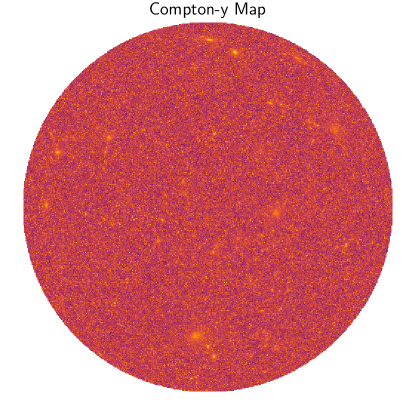
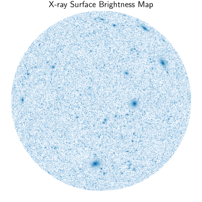
Figure 4: Half-sky Compton-$y$ map (left panel) and X-ray surface brightness map right panel) generated by applying the BP model to the Uchuu Lightcone. These maps are generated with triaxial halos but no intrinsic scatter. See Section 3 for more details.

3 Map Making

3.1 Uchuu Lightcone

The Uchuu Lightcone covers half of the sky from $0<z<2$. The lightcone is based on the Uchuu Simulation, a large-scale DM-only cosmological simulation with a box size of $(2\,h^{-1}{\rm Gpc})^{3}$ with DM particle resolution of $m_{p}=3.27\times 10^{8}\,h^{-1}M_{\odot}$ (Ishiyama et al., 2021). The simulation is performed assuming Planck cosmology with $\Omega_{m}=0.3089,\Omega_{b}=0.0486,n_{s}=0.9667,h=0.6774,\sigma_{8}=0.8159$, and $w=-1.0$. For the rest of the paper, we adopt the same cosmology unless stated otherwise. Halos and subhalos are identified by the ROCKSTAR code (Behroozi et al., 2013). Other Uchuu data products, such as mock galaxy catalogs based on Uchuu-UniverseMachine (Aung et al., 2023; Prada et al., 2023), Uchuu-$\nu^{2}$GC (Oogi et al., 2023), Uchuu-SDSS (Dong-Páez et al., 2024; Fernández-García et al., 2024), GLAM-Uchuu Lightcone (Ereza et al., 2024), and infrared sky SIDES-Uchuu (Gkogkou et al., 2023), are publicly available in the Skies $\&$ Universes database.

We used 27 snapshots between $z=0$ and $2$ of the Uchuu simulation to construct the half-sky Uchuu Lightcone. We place an observer in the simulation box and then transform the Cartesian coordinates of each halo into equatorial coordinates. The redshift of each halo is calculated by using the line-of-sight distance. We select halos between the redshift $(z_{i-1}+z_{i})/2$ and $(z_{i}+z_{i+1})/2$ in the given snapshot $i$, where $z_{i}$ is the redshift of this snapshot. Because the Uchuu $(2\,h^{-1}{\rm Gpc})^{3}$ volume is not enough to cover the half-sky spherical volume at a higher redshift, box replications are necessary. Instead of periodic replication, we apply three randomization transformations for each replica: the box rotation, mirroring, and translation (Blaizot et al., 2005; Bernyk et al., 2016), and then tile them to cover the spherical shell at a given snapshot. When the center of a halo lies close to the edge of a given spherical shell, it sometimes happens that the parts of subhalos of this halo do not lie within the shell. To ensure the hierarchy of halo and subhalo, we include such subhalos in the given shell. Finally, we join all spherical shells together to construct the half-sky lightcone.

The Uchuu Lightcone contains halos with a mass range of $M_{500c}\geq 10^{13}M_{\odot}$ and a redshift range of $0\leq z\leq 2$, with a total of $75,159,192$ halos. The lightcone catalog also contains information on the ratios of the halo axis $c/a$ and $b/a$, and the orientation of the major axis, derived from the ROCKSTAR halo catalog.

3.2 Generation of the Baryon Pasted Maps

We generate the maps in X-ray surface brightness in energy bands of $0.5-2$ keV and the tSZ Compton-$y$ maps in HEALPix (Hierarchical Equal Area and iso-Latitude Pixelization) (Górski et al., 2005) projection, with $N_{\rm side}=8192$, corresponding to angular pixel size of about $25.7$ arcseconds. We generate the maps by taking the RA, Dec, mass, and redshift provided in the Uchuu Lightcone catalog. We then map the RA and Dec positions of the 2D halo profile $\Sigma_{2D}(x^{\prime},y^{\prime})$ by determining which HEALPix pixels the profile belongs to, using the query_disc_inclusive and pix2ang functions provided by the HEALPix C++ package.

To study the impact of triaxiality and intrinsic scatter in X-ray and tSZ observables, we generated different realizations of the Compton-$y$ and X-ray surface brightness maps with the Uchuu Lightcone:

• spherical halos without intrinsic scatter (sph),

• triaxial halos with no intrinsic scatter (tri),

• spherical halos with intrinsic scatter (sph+var),

• triaxial halos with intrinsic scatter (tri+var),

with a total of 8 maps (4 X-ray Surface Brightness, 4 Compton-$y$). Details of the triaxial halo projection and intrinsic scatter modeling can be found in Sections 2.3 and 2.4, respectively. Note that no foreground or background noise is applied to these maps. Figure 4 shows the X-ray and Compton-$y$ maps with triaxiality but no intrinsic scatter (the ‘tri’ maps) in the gas profiles. Note that maps with triaxial halos with intrinsic scatter (‘tri+var’) overestimate the level of total scatter, since intrinsic scatter that we derived empirically from cosmological simulations does include the contribution from triaxiality. The scatter derived from this map thus provides an upper limit to the total amount of scatter expected from both intrinsic scatter and triaxiality.

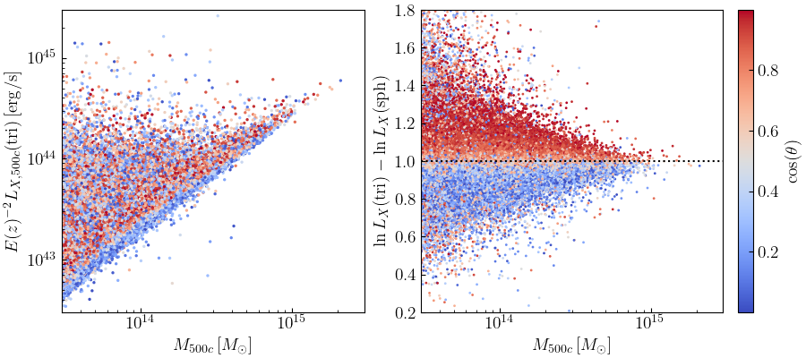
Figure 5: Left panel: X-ray luminosity-Mass scaling relation with the X-ray luminosity $L_{X}$ extracted from circular apertures with radii $R_{500c}$ in cluster-size halos $M_{500c}\geq 5\times 10^{13}M_{\odot}$ at $z<0.5$ from the X-ray Surface Brightness Uchuu BP Map, generated with halo triaxiality (the ‘tri’ map). The $E(z)^{-2}=H(z=0)/H(z)$ factor accounts for the self-similar redshift evolution of $L_{X}$. The color indicates the magnitude of $\cos(\theta)$, where $\theta$ is the angle between the major axis of the halo and the line-of-sight. for the halos in the baryon pasted maps. Right panel: the ratio between the $L_{X}$ in the ‘tri’ map, to that extracted from the spherical ‘sph’ map.

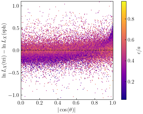
Figure 6: This plot shows the ratio between the $L_{X}$ extracted from the halos in the triaxial BP map (‘tri’), to that extracted from the spherical BP map (‘sph’), as a function of the orientation magnitude $\cos(\theta)$. The color indicates the minor-to-major axis ratio $c/a$.

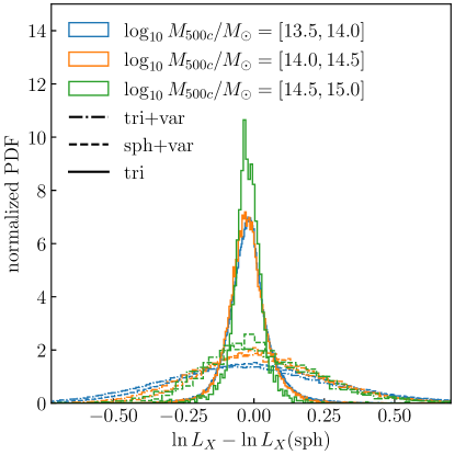
Figure 7: This plot shows the distribution of the $L_{X}$ extracted from the halos in the triaxial XSB map (‘tri’, solid lines), in the XSB map with spherical halos plus intrinsic scatter (‘sph+var’, dashed lines), and XSB map with triaxial halos with intrinsic scatter (‘tri+var’, dot-dasahed lines), to that extracted from the spherical BP XSB map (‘sph’), in different halo mass bins.

3.3 Performance, Memory and Storage Requirements

The BP map-making code is implemented in C++ and parallelized using Message Passing Interface (MPI), making it fast and efficient to generate maps with a large number of halos. The map-making approach presented in this paper is based on halo-by-halo, which is much faster than the particle-based approach presented in Osato & Nagai (2023), especially since each halo comprises at least 1000 DM particles. The code allocates halos across MPI tasks. Given the substantial number of halos ($75$ million) in the Uchuu lightcone, it is necessary to partition the lightcone into smaller parts to accommodate the data within the computer’s memory. We partitioned the Uchuu Lightcone into 40 redshift slices and generated maps separately for each slice independently, later combining them into one.

When we generated the map, we had to balance the number of cores allotted to each MPI task with the memory accessible per task. Allocating too many MPI tasks to a fixed number of nodes depletes the memory available for each task, while too few MPI tasks slow down the map-making process. On Yale’s Grace machine, featuring 48 cores (Intel XEON Icelake 2.40 GHz) and 480 GB of RAM per node, we allocated 16 MPI tasks across 16 nodes (one task per node). Consequently, projecting a single halo took about 2 minutes of wall time. This performance could be improved by assigning more MPI tasks per map with additional nodes. Regarding storage needs, for the BP-Uchuu map, the number of pixels is $N_{p}=12N_{\rm side}^{2}\approx 8\times 10^{8}$ with $N_{\rm side}=8192$, resulting in a map file size of approximately $6$ GB.

4 Results

4.1 Extrinsic Scatter in X-ray Luminosity–Halo Mass Scaling Relation

Figure 5 shows the impact of the triaxiality of the halo on the integrated X-ray luminosity $L_{X}$. The left panel shows the X–ray luminosity–mass scaling relation in the ‘tri’ XSB map. $L_{X}$ is measured within a circular aperture of radius $R_{500c}$ for each halo. The halos considered here have masses $M_{500c}\geq 5\times 10^{13}M_{\odot}$ and redshifts $z\leq 0.5$. The color of each data point represents the alignment of the triaxial halo with the line-of-sight, quantified by $\cos\theta$, where $\theta$ is the angle between the major axis of the halo and the line-of-sight. For a given mass, halos with lower values of $|\cos\theta|\lesssim 0.2$ generally exhibit lower values of $L_{X}$.

In the right panel, we show the comparison in $L_{X}$ between halos in the ‘tri’ and ‘sph’ maps. Each data point represents the difference in $\ln L_{x}$ measured from the ‘tri’ map to that from the ‘sph’ map for the same halo. This allows us to factor out the dependence on mass, as well as projection due to other halos (i.e., contamination from 2-halo terms), since the same halo on both maps is subject to the same projection. Halos with high $|\cos\theta|$ have $\ln L_{X}$ biased higher than those with low $|\cos\theta|$, and vice versa.

Figure 6 shows how the differences in $\ln L_{X}$ between ‘tri’ and ‘sph’ halos depend on $\cos\theta$ and the minor-to-major axis ratio $c/a$. It shows that the scatter due to triaxiality is driven mostly by elongated halos with low values of $c/a\lesssim 0.5$, dependent on their orientations: halos drive the bias high when their major axes are more aligned with the line-of-sight for $|\cos\theta|>0.8$, and the biases are lower when their major axes lie nearer to the plane of the sky for $|\cos\theta|<0.8$.

Figure 7 shows the distribution of $\Delta\ln L_{X}$ due to triaxiality, intrinsic scatter, and triaxiality plus intrinsic scatter from the ‘tri’, ‘sph+var’, and ‘tri+var’ maps, respectively. Using the $1\sigma$ standard deviation in $\Delta\ln L_{X}$ as the proxy for scatter, the cluster-sized halos with $\log_{10}(M_{500c}/M_{\odot})\in[14.5,15.0]$ have a scatter of $8\%$, which is comparable to the $9\%$ scatter in groups with $\log_{10}(M_{500c}/M_{\odot})\in[13.5,14.0]$ and less massive clusters with $\log_{10}(M_{500c}/M_{\odot})\in[14.0,14.5]$. The scatter due to triaxiality is subdominant to the intrinsic scatter, shown in dashed lines in the same figure. The intrinsic scatter is dependent on halo mass, peaking at $29\%$ for group-size halos and dropping to $20\%-22\%$ for cluster-size halos. When combining triaxiality and intrinsic scatter, the total scatter reaches $30\%$ for group-sized halos and $20\%$ for clusters.

Excluding halo core regions can significantly reduce intrinsic scatter in X-ray luminosity. By omitting pixels within a circular aperture of $0.2R_{500c}$ around each halo’s center, the intrinsic scatter decreases from $29\%$ to $22\%$ for groups and from $20\%$ to $11\%$ for massive clusters. However, the scatter due to triaxiality remains unchanged after core excision, maintaining at approximately $12\%$ at the group scale and $7\%$ at the cluster scale, constituting nearly half of the total scatter. These results indicate that the halo outskirts are the primary contributors to triaxial scatter.

Table 2 summarizes the scatter for all combinations of triaxiality and intrinsic scatter, with and without core excision.

	$\log_{10}(M_{500c}/M_{\odot})$
map type	$[13.5,14.0]$	$[14.0,14.5]$	$[14.5,15.0]$
Without core excision
tri	0.09	0.08	0.08
sph+var	0.29	0.22	0.20
tri+var	0.31	0.24	0.22
With core excision
tri	0.12	0.09	0.07
sph+var	0.22	0.15	0.11
tri+var	0.26	0.19	0.15

Table 2: $1\sigma$ scatter in $\ln L_{X}({\rm map\,type})-\ln L_{X}({\rm sph})$ for halos $z<0.5$ in different halo mass bins, with and without the core ($r<0.2R_{500c}$) excised.

4.2 Bias in X-ray and Thermal SZ Power Spectra due to Intrinsic Scatter in ICM Profiles

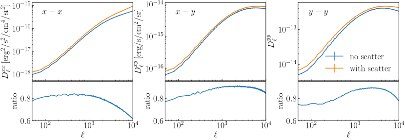
Figure 8: Plots showing the effect of intrinsic scatter of pressure and density profiles on the X-ray and tSZ auto- and cross-angular power spectra. The left, middle, and right panels show the X-ray auto-power spectra, X-ray/tSZ cross-power spectra, and tSZ auto-power spectra, measured from the Uchuu BP maps respectively. In each panel, the blue and orange lines represent the power spectra with and without intrinsic scatter in the halo profiles. The bottom sub-panels show the ratios of the power spectra with intrinsic scatter in the halo profiles, to those without. Note that the errorbars in each of the power spectrum are much smaller than the difference between the spectra. Also note that the tSZ auto-power spectrum is unit-less.

Figure 8 illustrates the X-ray and tSZ auto- and cross-angular power spectra derived from the ‘sph’ map (spherical halos with no intrinsic scatter) and the ‘sph+var’ map (spherical halos with intrinsic scatter). These spectra were computed with the anafast routine in healpy. We masked out $z<0.1$ halos to reduce non-Gaussian cosmic variance. The results demonstrate that intrinsic scatter in the density and pressure profiles significantly increases the power of both the X-ray and the tSZ angular power spectra in a scale-dependent way. Specifically, intrinsic scatter leads to = $20\%$ increase in the X-ray auto-power spectrum at small multipoles $\ell=100$, which increases to $40\%$ at $\ell=10^{4}$. The intrinsic scatter increases the tSZ auto-power spectrum by $25\%$ at $\ell=100$, by $10\%$ at $\ell=3000$, and by $20\%$ at $\ell=10^{4}$. The X-ray/tSZ cross-power spectrum shows a modest increase by $25\%$ at $\ell=100$, by $10\%$ at $\ell=3000$, and by $15\%$ at $\ell=10^{4}$. The contribution to the increase in power is dominated by massive halos $\log_{10}(M_{\rm vir}/M_{\odot})\geq 14.5$ at low redshift $z<0.5$. This rise in power due to intrinsic scatter in the gas profiles could potentially bias cosmological parameter estimates, particularly $\sigma_{8}$, which is sensitive to the normalization of the angular power spectrum. Using the $C_{\ell}\propto\sigma_{8}^{8.1}\Omega_{M}^{3.2}H_{0}^{-1.7}$ scaling (Bolliet et al., 2018), a change in the amplitude of the tSZ power spectrum $\Delta C_{\ell}/C_{\ell}\sim 25\%$ at $\ell\sim 100$ translates into bias in $\Delta\sigma_{8}/\sigma_{8}\sim 3\%$, $\Delta\Omega_{M}/\Omega_{M}\sim 8\%$, and $\Delta H_{0}/H_{0}\sim-15\%$, if the scatter in the thermal pressure profiles is neglected. Note that halo triaxiality has no effect on the measured power spectrum.

The observed increase in power can be interpreted as additional fluctuations resulting from halo-to-halo variations in pressure and density. To further explain this enhancement in angular power due to profile scatter, we provide a simple analytical framework using the halo model formalism. In the halo model, the angular power spectrum $C$ at a given multipole $\ell$, for two different observables $\cal A$ and $\cal B$ for halo at some mass $M$ and redshift $z$ is given by

$$C_{{\cal A}{\cal B}} = C^{\rm 1h}_{{\cal A}{\cal B}}+C^{\rm 2h}_{{\cal A}{\cal B}},$$ (30)

$$C^{\rm 1h}_{{\cal A}{\cal B}}(\ell) = \int{\rm d}z\frac{{\rm d}V}{{\rm d}z{\rm d}\Omega}\int{\rm d}M\frac{{\rm d}n}{{\rm d}M}$$

$$\times \left|{\cal A}_{\ell}(M,z){\cal B}_{\ell}(M,z)\right|,$$

$$C^{\rm 2h}_{{\cal A}{\cal B}}(\ell) = \int{\rm d}z\frac{{\rm d}V}{{\rm d}z{\rm d}\Omega}P_{\rm L}(k,z)$$

$$\times \left[\int{\rm d}M\frac{{\rm d}n}{{\rm d}M}{\cal A}_{\ell}(M,z)b(M,z)\right]$$

$$\times \left[\int{\rm d}M\frac{{\rm d}n}{{\rm d}M}{\cal B}_{\ell}(M,z)b(M,z)\right],$$

where $P_{\rm L}(k,z)$ is the linear matter power spectrum, ${\rm d}n/{\rm d}M$ is the halo mass function, and $b$ is the linear halo bias, and ${\cal A}_{\ell}$ and ${\cal B}_{\ell}$ are the Fourier transforms in multipole space of the observables $\cal A$ and $\cal B$ respectively. The angular power spectrum can be separated into the one-halo term $C^{\rm 1h}$ and the two-halo term $C^{\rm 2h}$ which represents the correlation between observables $\cal A$ and $\cal B$ within single halos and between two different halos, respectively. When the two observables are the same $\cal A=B$, then the angular power spectrum is called the auto-power spectrum; otherwise, it is the cross-power spectrum.

The angular power spectrum of clusters is dominated by the one-halo term $C^{\rm 1h}$ at most scales of interest ($\ell>10$), so we will ignore the two-halo term. The observables $\cal A$ and $\cal B$ for a halo in a given mass and redshift bin are expected to deviate from their expected value in that bin

$${\cal A} = \overline{\cal A}+\delta{\cal A},$$ (33)

$${\cal B} = \overline{\cal B}+\delta{\cal B}$$

where the overline indicates the expectation value and the $\delta$ terms indicate the deviation value which are treated as random variables. The $C^{\rm 1h}$ term then becomes

$$C^{\rm 1h}_{{\cal A}{\cal B}}(\ell) =\int{\rm d}z\frac{{\rm d}V}{{\rm d}z{\rm d}\Omega}\int{\rm d}M\frac{{\rm d}n}{{\rm d}M}$$

$$\times\left(\langle\overline{{\cal A}}^{*}_{\ell}(M,z)\overline{{\cal B}}_{\ell}(M,z)\rangle+\langle\delta{\cal A}^{*}_{\ell}(M,z)\delta{\cal B}_{\ell}(M,z)\rangle\right),$$

where $*$ superscript indicates the complex conjugate. Note that the terms ${\cal A}^{*}\delta{\cal B}$ and ${\cal B}\delta{\cal A}^{*}$ become zero when they are averaged. If there is a correlation between the variations of the two observables, expressed as $\langle\delta{\cal A}^{*}\delta{\cal B}\rangle\neq 0$, the implications are as follows: if $\langle\delta{\cal A}^{*}\delta{\cal B}\rangle>0$, this leads to an enhanced power spectrum, while $\langle\delta{\cal A}^{*}\delta{\cal B}\rangle<0$ results in a reduction of power. For the auto-power spectrum, $\langle\delta{\cal A}^{*}\delta{\cal A}\rangle=\langle|\delta{\cal A}|^{2}\rangle\geq 0$, indicating that any noticeable fluctuations in the observable will invariably increase the clustering power. In the X-ray/tSZ cross-power spectrum, we expect an increase in power, since X-ray surface brightness, which scales with the square of the gas density, correlates positively with thermal pressure contributing to the tSZ signal.

Interpretation of the power spectrum that uses the halo model usually overlooks the intrinsic scatter in halo gas profiles. As a result, the halo model approach typically underestimates the actual amplitude of the power spectrum. Thus, cosmological parameters, such as $S_{8}$, inferred through statistical inference based on the halo model, are often overestimated to account for the additional power from intrinsic scatter.

5 Discussion

Our findings are subject to several limitations that will be investigated further in future work. Firstly, the BP feedback model encapsulates the SNe and AGN feedback into one unified parameter. This approach does not adequately capture the intricate interactions occurring between SNe and AGN feedback (e.g., Medlock et al., 2024). Leveraging hydrodynamical cosmological simulations that incorporate varied SNe and AGN feedback physics across a broad spectrum of mass scales, such as those from CAMELS (Villaescusa-Navarro et al., 2021) and CarpoolGP (Lee et al., 2024), could enhance the feedback models applied in our study.

Secondly, one can improve the physicality in both the intrinsic and the extrinsic scatter models employed in this work. Intrinsic scatter stems from two main sources: (1) variations in the underlying DM matter distributions due to variations in the halo’s mass accretion histories (MAH) and (2) the stochastic feedback from AGN and SNe. The TNG300 simulation informs our model for intrinsic scatter, hence our model’s reliance on its specific cosmology and feedback prescriptions. To generalize this model, we must investigate how the intrinsic scatter varies for a range of cosmology and galaxy formation models using the CAMELS and CARPoolGP simulations.

Extrinsic scatter in our model is tied to the triaxiality of a halo gas, which is also calibrated using TNG300 and thus shares its limitations, notably its sensitivity to the cosmology and subgrid physics used in the simulation. Capturing the triaxial shape of a halo gas presents further challenges. The triaxial form of gas depends on that of the DM halo, and their relationship is influenced by baryonic physics (e.g., Kazantzidis et al., 2004; Lau et al., 2011; Machado et al., 2021). Moreover, the triaxiality of the DM halo is also shaped by its MAH (e.g., Lau et al., 2021). Consequently, modeling gas triaxiality requires a two-step methodology: (1) determining DM halo triaxiality using MAHs from simulations with varying cosmologies and (2) constructing a gas triaxial model based on the DM triaxial configuration using a series of cosmological simulations involving diverse baryonic physics. As weak lensing mass is also subjected to orientation bias (Becker & Kravtsov, 2011), this DM-gas triaxial model will enable us to account for scatter in scaling relations between weak lensing mass and gas observables (e.g., tSZ-weak lensing mass relation) due to the triaxial shape of the DM halo and its correlation with the gas shape.

6 Conclusions

In this work, we present X-ray Surface Brightness (XSB) and thermal Sunyaev-Zeldovich (tSZ) maps with the Baryon Pasting (BP) code, applying it to the half-sky lightcone derived from the Uchuu Cosmological $N$-body Simulations. These simulations encompass over $75$ million DM halos with masses $M_{500c}\geq 10^{13}M_{\odot}$, spanning a redshift range from $0$ to $2$. BP-Uchuu Maps facilitate the detection and evaluation of novel systematic effects in X-ray and SZ cosmological surveys at the map level. The vast sky coverage and large number of halos in the BP-Uchuu maps ensure that results are resilient to cosmic variance.

We demonstrated that the triaxial shape of the halo gas significantly affects the scatter in the X-ray luminosity versus halo mass relationship. In particular, the triaxial gas contributes $8\%-9\%$ to the scatter in X-ray luminosity at a given mass for group and cluster-size halos with $M_{500c}\geq 5\times 10^{13}M_{\odot}$, constituting nearly half of the total scatter in core-excised X-ray luminosity. This underscores the importance of its inclusion in standard cosmological analyses.

We further showed that the intrinsic scatter in the thermal pressure and gas density profiles enhances the clustering power in both the X-ray and tSZ auto- and cross-angular power spectra. The scatter in halo profiles results in a $20\%$ increase in the X-ray auto-power spectrum at small multipoles $\ell=100$, and increases to $40\%$ at $\ell=10^{4}$. The intrinsic scatter increases the tSZ auto-power spectrum by $25\%$ at $\ell=100$, by $10\%$ at $\ell=3000$, and by $20\%$ at $\ell=10^{4}$. The X-ray/tSZ cross power spectrum is minimally impacted, with an increase in power by $25\%$ at $\ell=100$, by $10\%$ at $\ell=3000$, and by $15\%$ at $\ell=10^{4}$. Ignoring this scatter in halo-model approaches could lead to biases in cosmological and astrophysical constraints with X-ray and tSZ power spectra.

The BP-Uchuu maps and halo catalog are available online for download via Globus. The BP map-making code is also available upon request.

7 Acknowledgements

This work is supported by NASA ATP23-0154 grant and the Yale Center for Research Computing. A.F. acknowledges support from the National Science Foundation under Cooperative Agreement AST-2421782. M.S. acknowledges support from MEXT KAKENHI Grant Number (20H05861, 23K19070, 24H00215, 24H00221). KO is supported by JSPS KAKENHI Grant Number JP22K14036 and JP24H00215. T.I. has been supported by IAAR Research Support Program in Chiba University Japan, MEXT/JSPS KAKENHI (Grant Number JP19KK0344 and JP23H04002), MEXT as “Program for Promoting Researches on the Supercomputer Fugaku” (JPMXP1020230406), and JICFuS. HM is supported by JSPS KAKENHI Grand Numbers JP20H01932, JP23H00108, and 22K21349, and Tokai Pathways to Global Excellence (T-GEx), part of MEXT Strategic Professional Development Program for Young Researchers We thank Instituto de Astrofisica de Andalucia (IAA-CSIC), Centro de Supercomputacion de Galicia (CESGA) and the Spanish academic and research network (RedIRIS) in Spain for hosting Uchuu DR1, DR2 and DR3 in the Skies & Universes site for cosmological simulations. The Uchuu simulations were carried out on Aterui II supercomputer at Center for Computational Astrophysics, CfCA, of National Astronomical Observatory of Japan, and the K computer at the RIKEN Advanced Institute for Computational Science. The Uchuu Data Releases efforts have made use of the skun@IAA_RedIRIS and skun6@IAA computer facilities managed by the IAA-CSIC in Spain (MICINN EU-Feder grant EQC2018-004366-P).

Appendix A Validation of the BP model with Observations and Simulations

A.1 Profile Comparison

In this section, we compare the gas density and pressure profiles of the fiducial BP model against cosmological simulations and observations.

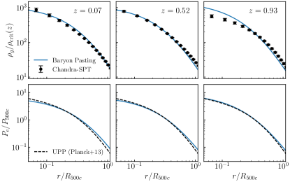
Figure 9: Comparison of profiles of gas density (top panels) and electron thermal pressure (bottom panels) with the BP model with default gas parameters for $M_{500c}=5\times 10^{14}M_{\odot}$ at $z=0.07,0.52,0.93$ (left, middle, right panels), with with the Universal Pressure profile from Planck Collaboration et al. (2013) (dashed black line) and the density profile measurements from Chandra-SPT cluster sample presented in Flender et al. (2017) as black data points with 1$\sigma$ errorbars.

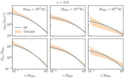
Figure 10: Comparision of the best-fit BP model (blue solid lines) to the gas density (top panels) and thermal pressure (bottom panels) of the TNG300 simulations for $\log_{10}(M_{500c}/M_{\odot})=13,14,15$ at $z=0$. The shaded regions represent $\pm 1\sigma$ of around the mean profile of the TNG300 halos.

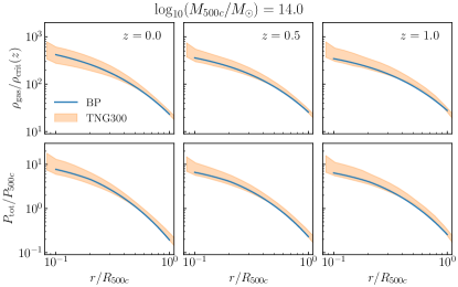
Figure 11: Same as Figure 10, but for $\log_{10}(M_{500c}/M_{\odot})=14.0$ $z=0.0,0.5,1.0$ (from left to right).

Figure 9 shows the comparison of thermal pressure and gas density profiles of the BP Model to observations. In the top panels, we show the comparison between average gas density profile of clusters at $z=0.07,0.52,0.93$ from the Chandra-SPT cluster sample, to that of the BP model of a halo with mass $M_{500c}=6\times 10^{14}M_{\odot}$. There is a very good agreement between the BP model and the Chandra measurements. This is not surprising given that the BP model is calibrated with the density profiles of the Chandra-SPT clusters (Flender et al., 2017).

In the bottom panels of the same figure, we compare the Universal Pressure Profile between the Planck-XMM measurements (Planck Collaboration et al., 2013) and the BP model for the same halos. Again there is good agreement between the profiles of the BP model and the Universal Pressure Profile. Note that we do not fit the BP model to the Planck-XMM data. All the model parameters are from our calibration with the Chandra-SPT data, except the inner Polytropic index where we change from the fiducial value of $0.10$ to $1.0$. Note that the thermal pressure profiles are normalized by $P_{500c}=1.45\times 10^{-11}\,{\rm erg\,cm^{-3}}\left(\frac{f_{b}}{0.174}\right)\left(\frac{h}{0.7}\right)^{2}E(z)^{8/3}\left(\frac{M_{500c}}{10^{15}h^{-1}M_{\odot}}\right)^{2/3}$ to account for self-similar mass and redshift dependence in the normalization of the pressure profile.

Figure 10 shows the comparison of thermal pressure and gas density profiles from the TNG300 simulation (Nelson et al., 2019) at different halo masses $\log_{10}(M_{500c}/M_{\odot})=(13,14,15)$ at $z=0$, and the corresponding profiles of the best-fit BP model. Figure 11 shows the same profiles for $\log_{10}(M_{500c}/M_{\odot})=14$ at $z=0,0.5,1$. Note that we fix the $f_{\star}=0.019$ and $S_{\star}=0.16$ to those corresponding to the TNG300 simulations. The good agreement between the simulation and the BP model profiles for wide range of halo masses and redshifts demonstrates the flexibility of the BP model in describing thermodynamic profiles in cosmological simulations.

A.2 tSZ angular power spectrum

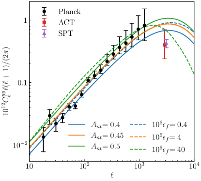
Figure 12: tSZ angular power spectra using the halo model in BP, with varying non-thermal pressure fraction parameter $A_{\rm nt}$. We also plot the Planck tSZ power spectrum (Planck Collaboration et al., 2016) in black with 1$\sigma$ errorbars for comparison. The model power spectrum with the fiducial $A_{\rm nt}=0.45$ and $10^{6}\epsilon_{f}=4.0$ agrees well with the mean power spectrum from Planck. The observation uncertainties can be bracketed with model power spectra with $A_{\rm nt}=\{0.40,0.50\}$.

In Figure 12 we compare the Halo model-based tSZ power spectra computed with the BP code to the tSZ power spectrum from Planck (Planck Collaboration et al., 2016), ACT, and SPT. The BP tSZ power spectrum is computed with mass range $\log_{10}(M_{\rm vir}/M_{\odot})=[13,16]$ and redshift range $z=[0.0,2.0]$, following Equations (39)-(42) in Osato & Nagai (2023), with varying non-thermal pressure fraction parameter $A_{\rm nt}$. We use the Planck 2018 cosmology (Planck Collaboration et al., 2020) to compute the power spectrum. We compare the model power spectra with that of Planck from Planck Collaboration et al. (2016). The BP tSZ power spectrum with the fiducial non-thermal pressure fraction parameter $A_{\rm nt}=0.45$ calibrated from cosmological hydrodynamical simulation provides a good match to the Planck measurements. This is also consistent with previous works that compared the BP model power spectra with observations (Osato et al., 2018).

References

- Agarwal et al. (2018) Agarwal, S., Davé, R., & Bassett, B. A. 2018, Monthly Notices of the Royal Astronomical Society, 478, 3410
- Allen et al. (2011) Allen, S. W., Evrard, A. E., & Mantz, A. B. 2011, ARA&A, 49, 409, doi: 10.1146/annurev-astro-081710-102514
- Asplund et al. (2009) Asplund, M., Grevesse, N., Sauval, A. J., & Scott, P. 2009, ARA&A, 47, 481, doi: 10.1146/annurev.astro.46.060407.145222
- Aung et al. (2021) Aung, H., Nagai, D., & Lau, E. T. 2021, MNRAS, 508, 2071, doi: 10.1093/mnras/stab2598
- Aung et al. (2023) Aung, H., Nagai, D., Klypin, A., et al. 2023, MNRAS, 519, 1648, doi: 10.1093/mnras/stac3514
- Battaglia et al. (2012) Battaglia, N., Bond, J. R., Pfrommer, C., & Sievers, J. L. 2012, ApJ, 758, 74, doi: 10.1088/0004-637X/758/2/74
- Bayer et al. (2024) Bayer, A. E., Zhong, Y., Li, Z., et al. 2024, arXiv e-prints, arXiv:2407.17462, doi: 10.48550/arXiv.2407.17462
- Becker & Kravtsov (2011) Becker, M. R., & Kravtsov, A. V. 2011, ApJ, 740, 25, doi: 10.1088/0004-637X/740/1/25
- Behroozi et al. (2019) Behroozi, P., Wechsler, R. H., Hearin, A. P., & Conroy, C. 2019, Monthly Notices of the Royal Astronomical Society, 488, 3143
- Behroozi et al. (2013) Behroozi, P. S., Wechsler, R. H., & Wu, H.-Y. 2013, ApJ, 762, 109, doi: 10.1088/0004-637X/762/2/109
- Benson et al. (2013) Benson, B. A., de Haan, T., Dudley, J. P., et al. 2013, ApJ, 763, 147, doi: 10.1088/0004-637X/763/2/147
- Bernyk et al. (2016) Bernyk, M., Croton, D. J., Tonini, C., et al. 2016, ApJS, 223, 9, doi: 10.3847/0067-0049/223/1/9
- Blaizot et al. (2005) Blaizot, J., Wadadekar, Y., Guiderdoni, B., et al. 2005, MNRAS, 360, 159, doi: 10.1111/j.1365-2966.2005.09019.x
- Bocquet et al. (2019) Bocquet, S., Dietrich, J., Schrabback, T., et al. 2019, The Astrophysical Journal, 878, 55
- Bolliet et al. (2018) Bolliet, B., Comis, B., Komatsu, E., & Macías-Pérez, J. F. 2018, MNRAS, 477, 4957, doi: 10.1093/mnras/sty823
- Bryan & Norman (1998) Bryan, G. L., & Norman, M. L. 1998, ApJ, 495, 80, doi: 10.1086/305262
- Chadayammuri et al. (2023) Chadayammuri, U., Ntampaka, M., ZuHone, J., Bogdán, Á., & Kraft, R. P. 2023, MNRAS, 526, 2812, doi: 10.1093/mnras/stad2596
- Clerc et al. (2018) Clerc, N., Ramos-Ceja, M., Ridl, J., et al. 2018, Astronomy & Astrophysics, 617, A92
- Comparat et al. (2020) Comparat, J., Eckert, D., Finoguenov, A., et al. 2020, The Open Journal of Astrophysics, 3, 13, doi: 10.21105/astro.2008.08404
- Costanzi et al. (2019) Costanzi, M., Rozo, E., Simet, M., et al. 2019, Monthly Notices of the Royal Astronomical Society, 488, 4779
- Dong-Páez et al. (2024) Dong-Páez, C. A., Smith, A., Szewciw, A. O., et al. 2024, MNRAS, doi: 10.1093/mnras/stae062
- Ereza et al. (2024) Ereza, J., Prada, F., Klypin, A., et al. 2024, MNRAS, 532, 1659, doi: 10.1093/mnras/stae1543
- Farahi et al. (2022) Farahi, A., Anbajagane, D., & Evrard, A. E. 2022, The Astrophysical Journal, 931, 166
- Farahi et al. (2018) Farahi, A., Evrard, A. E., McCarthy, I., Barnes, D. J., & Kay, S. T. 2018, MNRAS, 478, 2618, doi: 10.1093/mnras/sty1179
- Farahi et al. (2019) Farahi, A., Mulroy, S. L., Evrard, A. E., et al. 2019, Nature Communications, 10, 2504, doi: 10.1038/s41467-019-10471-y
- Farahi et al. (2019) Farahi, A., Chen, X., Evrard, A., et al. 2019, Monthly Notices of the Royal Astronomical Society, 490, 3341
- Fernández-García et al. (2024) Fernández-García, E., Betancort-Rijo, J. E., Prada, F., Ishiyama, T., & Klypin, A. 2024, arXiv e-prints, arXiv:2406.13736, doi: 10.48550/arXiv.2406.13736
- Flender et al. (2017) Flender, S., Nagai, D., & McDonald, M. 2017, ApJ, 837, 124, doi: 10.3847/1538-4357/aa60bf
- Foster et al. (2012) Foster, A. R., Ji, L., Smith, R. K., & Brickhouse, N. S. 2012, ApJ, 756, 128, doi: 10.1088/0004-637X/756/2/128
- Ghirardini et al. (2019) Ghirardini, V., Eckert, D., Ettori, S., et al. 2019, A&A, 621, A41, doi: 10.1051/0004-6361/201833325
- Gkogkou et al. (2023) Gkogkou, A., Béthermin, M., Lagache, G., et al. 2023, A&A, 670, A16, doi: 10.1051/0004-6361/202245151
- Górski et al. (2005) Górski, K. M., Hivon, E., Banday, A. J., et al. 2005, ApJ, 622, 759, doi: 10.1086/427976
- Hadzhiyska et al. (2020) Hadzhiyska, B., Bose, S., Eisenstein, D., Hernquist, L., & Spergel, D. N. 2020, Monthly Notices of the Royal Astronomical Society, 493, 5506
- Hurier et al. (2015) Hurier, G., Douspis, M., Aghanim, N., et al. 2015, A&A, 576, A90, doi: 10.1051/0004-6361/201425555
- Ishiyama et al. (2021) Ishiyama, T., Prada, F., Klypin, A. A., et al. 2021, MNRAS, 506, 4210, doi: 10.1093/mnras/stab1755
- Kazantzidis et al. (2004) Kazantzidis, S., Kravtsov, A. V., Zentner, A. R., et al. 2004, ApJ, 611, L73, doi: 10.1086/423992
- Kéruzoré et al. (2024) Kéruzoré, F., Bleem, L. E., Frontiere, N., et al. 2024, arXiv e-prints, arXiv:2408.17445, doi: 10.48550/arXiv.2408.17445
- Kim et al. (2024) Kim, J., Sayers, J., Sereno, M., et al. 2024, A&A, 686, A97, doi: 10.1051/0004-6361/202347399
- Komatsu & Seljak (2001) Komatsu, E., & Seljak, U. 2001, MNRAS, 327, 1353, doi: 10.1046/j.1365-8711.2001.04838.x
- Lau et al. (2023) Lau, E. T., Bogdán, Á., Chadayammuri, U., et al. 2023, MNRAS, 518, 1496, doi: 10.1093/mnras/stac3147
- Lau et al. (2024) Lau, E. T., Bogdán, Á., Nagai, D., Cappelluti, N., & Shirasaki, M. 2024. https://arxiv.org/abs/2410.22397
- Lau et al. (2021) Lau, E. T., Hearin, A. P., Nagai, D., & Cappelluti, N. 2021, MNRAS, 500, 1029, doi: 10.1093/mnras/staa3313
- Lau et al. (2011) Lau, E. T., Nagai, D., Kravtsov, A. V., & Zentner, A. R. 2011, ApJ, 734, 93, doi: 10.1088/0004-637X/734/2/93
- Lee et al. (2024) Lee, M. E., Genel, S., Wandelt, B. D., et al. 2024, ApJ, 968, 11, doi: 10.3847/1538-4357/ad3d4a
- Limousin et al. (2013) Limousin, M., Morandi, A., Sereno, M., et al. 2013, Space Science Reviews, 177, 155
- Machado et al. (2021) Machado, L. F., Avestruz, C., Barnes, D. J., et al. 2021, MNRAS, 507, 1468, doi: 10.1093/mnras/stab2252
- Mantz et al. (2010) Mantz, A., Allen, S. W., Ebeling, H., Rapetti, D., & Drlica-Wagner, A. 2010, Monthly Notices of the Royal Astronomical Society, 406, 1773
- Mantz et al. (2016) Mantz, A. B., Allen, S. W., Morris, R. G., et al. 2016, Monthly Notices of the Royal Astronomical Society, 463, 3582
- Mead et al. (2021) Mead, A., Brieden, S., Tröster, T., & Heymans, C. 2021, Monthly Notices of the Royal Astronomical Society, 502, 1401
- Medlock et al. (2024) Medlock, I., Neufeld, C., Nagai, D., et al. 2024, arXiv e-prints, arXiv:2410.16361, doi: 10.48550/arXiv.2410.16361
- Mernier et al. (2018) Mernier, F., Biffi, V., Yamaguchi, H., et al. 2018, Space Sci. Rev., 214, 129, doi: 10.1007/s11214-018-0565-7
- More et al. (2015) More, S., Diemer, B., & Kravtsov, A. V. 2015, ApJ, 810, 36, doi: 10.1088/0004-637X/810/1/36
- Moster et al. (2018) Moster, B. P., Naab, T., & White, S. D. 2018, Monthly Notices of the Royal Astronomical Society, 477, 1822
- Mulroy et al. (2019) Mulroy, S. L., Farahi, A., Evrard, A. E., et al. 2019, Monthly Notices of the Royal Astronomical Society, 484, 60
- Navarro et al. (1996) Navarro, J. F., Frenk, C. S., & White, S. D. M. 1996, ApJ, 462, 563, doi: 10.1086/177173
- Nelson et al. (2019) Nelson, D., Springel, V., Pillepich, A., et al. 2019, Computational Astrophysics and Cosmology, 6, 2, doi: 10.1186/s40668-019-0028-x
- Nelson et al. (2014a) Nelson, K., Lau, E. T., & Nagai, D. 2014a, ApJ, 792, 25, doi: 10.1088/0004-637X/792/1/25
- Nelson et al. (2014b) Nelson, K., Lau, E. T., Nagai, D., Rudd, D. H., & Yu, L. 2014b, ApJ, 782, 107, doi: 10.1088/0004-637X/782/2/107
- Nguyen et al. (2024) Nguyen, T., Villaescusa-Navarro, F., Mishra-Sharma, S., et al. 2024, arXiv preprint arXiv:2409.02980
- Omori (2022) Omori, Y. 2022, arXiv e-prints, arXiv:2212.07420, doi: 10.48550/arXiv.2212.07420
- Oogi et al. (2023) Oogi, T., Ishiyama, T., Prada, F., et al. 2023, MNRAS, 525, 3879, doi: 10.1093/mnras/stad2401
- Osato et al. (2018) Osato, K., Flender, S., Nagai, D., Shirasaki, M., & Yoshida, N. 2018, MNRAS, 475, 532, doi: 10.1093/mnras/stx3215
- Osato & Nagai (2023) Osato, K., & Nagai, D. 2023, MNRAS, 519, 2069, doi: 10.1093/mnras/stac3669
- Ostriker et al. (2005) Ostriker, J. P., Bode, P., & Babul, A. 2005, ApJ, 634, 964, doi: 10.1086/497122
- Planck Collaboration et al. (2013) Planck Collaboration, Ade, P. A. R., Aghanim, N., et al. 2013, A&A, 550, A131, doi: 10.1051/0004-6361/201220040
- Planck Collaboration et al. (2016) Planck Collaboration, Aghanim, N., Arnaud, M., et al. 2016, A&A, 594, A22, doi: 10.1051/0004-6361/201525826
- Planck Collaboration et al. (2020) Planck Collaboration, Aghanim, N., Akrami, Y., et al. 2020, A&A, 641, A6, doi: 10.1051/0004-6361/201833910
- Pop et al. (2022) Pop, A.-R., Hernquist, L., Nagai, D., et al. 2022, arXiv e-prints, arXiv:2205.11528, doi: 10.48550/arXiv.2205.11528
- Prada et al. (2023) Prada, F., Behroozi, P., Ishiyama, T., Klypin, A., & Pérez, E. 2023, arXiv e-prints, arXiv:2304.11911, doi: 10.48550/arXiv.2304.11911
- Pratt et al. (2019) Pratt, G. W., Arnaud, M., Biviano, A., et al. 2019, Space Sci. Rev., 215, 25, doi: 10.1007/s11214-019-0591-0
- Schaye et al. (2023) Schaye, J., Kugel, R., Schaller, M., et al. 2023, MNRAS, 526, 4978, doi: 10.1093/mnras/stad2419
- Seljak (2000) Seljak, U. 2000, Monthly Notices of the Royal Astronomical Society, 318, 203
- Sereno et al. (2020) Sereno, M., Umetsu, K., Ettori, S., et al. 2020, Monthly Notices of the Royal Astronomical Society, 492, 4528
- Shaw et al. (2010) Shaw, L. D., Nagai, D., Bhattacharya, S., & Lau, E. T. 2010, ApJ, 725, 1452, doi: 10.1088/0004-637X/725/2/1452
- Shirasaki et al. (2020) Shirasaki, M., Lau, E. T., & Nagai, D. 2020, MNRAS, 491, 235, doi: 10.1093/mnras/stz3021
- Stark (1977) Stark, A. A. 1977, ApJ, 213, 368, doi: 10.1086/155164
- Stein et al. (2020) Stein, G., Alvarez, M. A., Bond, J. R., van Engelen, A., & Battaglia, N. 2020, J. Cosmology Astropart. Phys, 2020, 012, doi: 10.1088/1475-7516/2020/10/012
- Truong et al. (2018) Truong, N., Rasia, E., Mazzotta, P., et al. 2018, MNRAS, 474, 4089, doi: 10.1093/mnras/stx2927
- Valotti et al. (2018) Valotti, A., Pierre, M., Farahi, A., et al. 2018, Astronomy & Astrophysics, 614, A72
- Vikhlinin et al. (2009) Vikhlinin, A., Kravtsov, A. V., Burenin, R. A., et al. 2009, ApJ, 692, 1060, doi: 10.1088/0004-637X/692/2/1060
- Villaescusa-Navarro et al. (2021) Villaescusa-Navarro, F., Anglés-Alcázar, D., Genel, S., et al. 2021, ApJ, 915, 71, doi: 10.3847/1538-4357/abf7ba
- Wechsler & Tinker (2018) Wechsler, R. H., & Tinker, J. L. 2018, Annual Review of Astronomy and Astrophysics, 56, 435
- Williams et al. (2023) Williams, I. M., Khan, A., & McQuinn, M. 2023, MNRAS, 520, 3626, doi: 10.1093/mnras/stad293
- Yang et al. (2022) Yang, T., Cai, Y.-C., Cui, W., et al. 2022, MNRAS, 516, 4084, doi: 10.1093/mnras/stac2505
- Zandanel et al. (2018) Zandanel, F., Fornasa, M., Prada, F., et al. 2018, MNRAS, 480, 987, doi: 10.1093/mnras/sty1901
- Zhang et al. (2024) Zhang, Z., Farahi, A., Nagai, D., et al. 2024, MNRAS, 530, 3127, doi: 10.1093/mnras/stae999
- Zonca et al. (2019) Zonca, A., Singer, L., Lenz, D., et al. 2019, The Journal of Open Source Software, 4, 1298, doi: 10.21105/joss.01298