The quark gap equation in light-cone gauge

Abstract

We calculate the quark self-energy correction in light-cone gauge motivated by distribution amplitudes whose definition implies a Wilson line. The latter serves to preserve the gauge invariance of the hadronic amplitudes and becomes trivial in light-cone gauge. Therefore, the calculation of the distribution amplitudes simplifies significantly provided that wave functions and propagators are obtained in that gauge. In here, we explore the corresponding Dyson-Schwinger equation in its leading truncation and with a dressed vertex derived from a Ward identity in light-cone gauge. The quark’s mass and wave renormalization functions, as well as a third complex-valued amplitude, are found to depend on the relative orientation of the quark momentum and a light-like four-vector, which expresses a geometric gauge dependence of the propagator.

I Introduction

Noncovariant gauges have a long history and, as their name implies, one of their features is the breaking of relativistic covariance. A typical example is provided by the light-cone gauge, which is a noncovariant physical gauge defined by,

$$n\cdot A^{a}=0\,,$$ (1)

where $A^{a}_{\mu}(x)$ is a massless Yang-Mills field and $n_{\mu}$ is a light-like four-vector defined by $n^{2}=0$. Since the four-vector $n$ defines a preferential axis in space-time, the above condition is more generally referred to as axial gauge. Despite the lack of covariance, the strong interest in axial gauges can be attributed to the decoupling of the Faddeev-Popov ghosts from the gauge field, thereby eliminating the unphysical degrees of freedom in the theory Leibbrandt:1987qv . This is because the ghost-gluon vertex is proportional to the vector $n$ which projects out the gluon fields due to the gauge condition in Eq. (1). Consequently, $n^{\mu}D_{\mu\nu}^{ab}=0$ in any Feynman diagram, where $D_{\mu\nu}^{ab}$ is the gluon propagator in light-cone gauge. This observation alone may be of interest to the nonperturbative calculation of the gluon propagator Aguilar:2006gr ; Aguilar:2008xm , as the gluon also decouples from the ghost in the Dyson-Schwinger equation (DSE).

There are other reasons to consider light-cone gauge, in particular when facing the difficulty of evaluating nonperturbative matrix elements that contain a Wilson line Costa:2021mpk . The phenomenological motivation stems from the definition of light-cone distribution amplitudes and parton distribution functions Jaffe:1996zw , which contain a Wilson line to preserve gauge symmetry. More precisely, there exists a body of work that addresses parton distribution within a DSE and Bethe-Salpeter equation approach of the mesons in Landau gauge, assuming the effect of the Wilson line is negligible Serna:2020txe ; Serna:2022yfp ; Chang:2013pq ; Shi:2015esa . An alternative approach is to project the Bethe-Salpeter wave function on the light front and derive therefrom mesonic distributions functions, which avoids the Wilson line altogether but is so far limited to the leading Fock state Mezrag:2016hnp ; Shi:2018zqd ; Serna:2024vpn .

The parton distribution function of a pseudoscalar mesons is defined as,

$$q_{M}(x)= \int\frac{d\lambda}{4\pi}\,e^{-ix\lambda P\cdot n}$$

$$\times\,\langle M|\bar{\psi}_{q}(0)\gamma\cdot n\,W(0,\lambda n)\psi_{q}(\lambda n)|M\rangle\,,$$ (2)

where $x=k\cdot n/P\cdot n$ is the light-cone momentum fraction carried by the struck quark and the Wilson line reads,

$$W(0,n\lambda)=\mathcal{P}e^{-ig\int_{\lambda}^{0}n\,\cdot A(n\xi)d\xi}\,,$$ (3)

in which $\mathcal{P}$ denotes the path-ordering operator. In light-cone gauge (1) this operator is trivial, which is why the calculation of distributions is attractive in this gauge. However, this comes at a price: the necessity to calculate nonperturbative quark propagators in light-cone gauge. In a functional continuum approach to Quantum Chromodynamics (QCD), this is commonly done by solving the respective DSEs of the fermion and gauge fields in Landau or covariant $R_{\xi}$ gauges Lessa:2022wqc .

In here, we take a first step to fill this gap and solve the quark DSE in light-cone gauge. We start with the general form of the quark propagator and discuss divergences in Feynman diagrams that stem from the denominator $(n\cdot q)^{-1}$ in the gluon propagator. We then formulate the DSE of the quark in light-cone gauge and address this issue within this nonperturbative framework. The solution can be decomposed into three Lorentz-invariant amplitudes, two of which are real and play the role of the mass and wave function renormalization known of covariant gauges, while the third amplitude is complex. It is found that all amplitudes exhibit an angular dependence on the light-like vector $n$. We interpret this behavior as a geometric expression of gauge dependence of the quark propagator in light-cone gauge.

II Gluon propagator in light-cone gauge

The light-cone gauge  (1) is implemented with a gauge fixing term restricting the degrees of freedom in the QCD Lagrangian,

$$\mathcal{L}_{\text{fix}}=-\frac{1}{2\alpha}\left(n\cdot A^{a}\right)^{2},$$ (4)

From the Yang-Mills Lagrangian and the gauge fixing term (4) one can derive the Euler-Lagrange equation of a non-interacting gluon. After taking $\alpha\to 0$, this leads to the Green function,

$$D_{\mu\nu}^{ab}(q)=\frac{-i\delta^{ab}}{q^{2}+i\epsilon}\left(g_{\mu\nu}-\frac{n_{\mu}q_{\nu}+n_{\nu}q_{\mu}}{n\cdot q}\right)\,,$$ (5)

which is the gluon propagator in light-cone gauge that satisfies,

$$n^{\mu}D_{\mu\nu}(q)=n^{\nu}D_{\mu\nu}(q)=0\,.$$ (6)

Any Feynman diagram containing a gluon propagator (5) also includes the $(n\cdot q)^{-1}$ pole. Divergences arising from this pole can be dealt with using a principal value prescription, though an attractive alternative is offered by the Mandelstam-Leibbrandt [ML] prescription Leibbrandt:1983pj ; Leibbrandt:1987uc ; Mandelstam:1982cb . The latter modifies the denominator by adding a small imaginary shift $i\theta$ which is taken to zero after Wick rotation. In order to do so, the denominator must be put in a form that allows for a Wick rotation without hitting poles. The ML prescription rests on the observation that the definition of a light-like vector with $n^{2}=0$ does not constrain the vector unambigously:

$$n_{0}^{2}-\vec{n}^{\,2}=0\ \ \Longrightarrow\ \ n_{0}=\pm|\vec{n}|\,.$$ (7)

Therefore, the location of the $(n\cdot q)^{-1}$ pole is not unique. This ambiguity can be addressed by choosing $n=(|\vec{n}|,\vec{n})$ and introducing a dual vector $n^{*}=(|\vec{n}|,-\vec{n})$, $n^{*2}=0$, $n^{*}\cdot n>0$. According to Ref. Leibbrandt:1983pj , the ML prescription is then given by,

$$\frac{1}{n\cdot q}=\,\lim_{\theta\rightarrow 0}\frac{n^{*}\!\cdot q}{\left(n^{*}\!\cdot q\right)(n\cdot q)+i\theta}\,.$$ (8)

where $\theta>0$. In an integral the prescription leads to,

$$\int d^{4}q \,\frac{n^{*}\!\cdot q}{\left(n^{*}\!\cdot q\right)(n\cdot q)+i\theta}$$

$$=\int d^{4}q \,\frac{n^{*}\!\cdot q}{n_{0}^{2}\left(q_{0}^{2}-\frac{(\vec{n}\cdot\vec{q}\,)^{2}}{n_{0}^{2}}+\frac{i\theta}{n_{0}^{2}}\right)}\ ,$$ (9)

from which can be read that the poles are located in the second and fourth quadrants,

$$q_{0}=\frac{1}{n_{0}}\left(\pm|\vec{n}\cdot\vec{q}\,|\mp i\frac{\theta}{2|\vec{n}\cdot\vec{q}\,|}\right)\,.$$ (10)

This allows for a Wick rotation using a counter-clockwise path realized with the Euclidian ML prescription,

$$\left(\frac{1}{n\cdot q}\right)_{\!E}=\lim_{\theta^{2}\to 0}\ \frac{(n^{*}\!\cdot q)_{E}}{(n^{*}\!\cdot q)_{E}\,(n\cdot q)_{E}+\theta^{2}}\ ,$$ (11)

where $n_{0}=in_{4}=in_{4}^{*}$, $q^{2}=-q_{E}^{2}$ and $n\cdot q=-(n\cdot q)_{E}$.

When a diagram includes gluon and quark propagators, the corresponding integral contains three types of poles, all of which are located in the second and fourth quadrants of the complex plane. Therefore, in calculating the self-energy correction of the quark propagator at one loop, a Wick rotation to Euclidean space is straightforward.

At one-loop order, the trace of the quark self-energy $\Sigma(p,n,n^{*})$ leads to a tensor structure whose most general decomposition is given by the sum Leibbrandt:1983zd ; Mirja2020 ,

$$\Sigma(p,n,n^{*}) =a\,i\gamma\cdot p+b\,\mathbb{1}+c\,i\gamma\cdot n$$

$$-d\,i(\gamma\cdot n\,\gamma\cdot n^{*}\gamma\cdot p+\gamma\cdot p\ \gamma\cdot n^{*}\gamma\cdot n)\,,$$ (12)

and all vectors and Dirac matrices are now in Euclidean space. The $d$-term stems from the regularization procedure and can be further reduced to amplitudes proportional to $p$, $n$ and $n^{*}$ using the identity,

$$\gamma\cdot n\,\gamma \cdot n^{*}\gamma\cdot p+\gamma\cdot p\,\gamma\cdot n^{*}\gamma\cdot n$$

$$= \ (2\,n^{*}\!\cdot p)\gamma\cdot n-(2\,n\cdot p)\gamma\cdot n^{*}\!+(2\,n^{*}\!\!\cdot n)\gamma\cdot p\,,$$ (13)

which simplifies Eq. (12) to:

$$\Sigma(p,n,n^{*})=A\,i\gamma\cdot p+B\,\mathbb{1}+C\,i\gamma\cdot n+D\,i\gamma\cdot n^{*}\,.\\$$ (14)

The structure of Eq. (14) can be understood within the framework of the Newman-Penrose tetrad scheme Newman:1961qr , in which any four-dimensional vector can be represented in terms of four null vectors, and is discussed in detail in Ref. Leibbrandt:1984be .

Appropriate projections allow to obtain integral equations for all four amplitudes, $A,B,C$ and $D$, and in a one-loop calculation they can be solved with the usual Feynman parametrizations, though the four equations remain uncoupled. In a nonperturbative functional approach based on the DSE, the amplitudes are described by a set of nonlinear coupled integral equations. We numerically solve this system of equations in light-cone gauge and discuss their solutions in the following sections.

III Gap equation in light-cone gauge

For the phenomenological reasons expounded in Section I, we are interested in nonperturbative quark propagators which are solutions of the quark gap equation. To this end, we solve the equation of motion of the quark, which in quantum field theory is known as DSE. For the quark of a given flavor the inverse quark propagator is obtained from,

$$S^{-1}(p) =\,Z_{2}\,i\,\gamma\cdot p+Z_{4}\,m(\mu)$$

$$+\,Z_{1} g^{2}\int^{\Lambda}\!\!\frac{d^{4}k}{(2\pi)^{4}}\ D^{ab}_{\mu\nu}(q)\,\gamma_{\mu}t^{a}\,S(k)\,\Gamma_{\nu}^{b}(k,p)\,,$$ (15)

where $q=k-p$ is the gluon momentum, $Z_{1}(\mu,\Lambda)$, $Z_{2}(\mu,\Lambda)$ and $Z_{4}(\mu,\Lambda)$ are the vertex, wave function and mass renormalization constants, respectively, $m(\mu)$ is the renormalized current-quark mass and $t^{a}=\lambda^{a}/2$ are the SU(3) group generators. In the self-energy integral, $\Lambda$ is a Poincaré-invariant cut-off while $\mu$ is the renormalization point chosen such that $\Lambda\gg\mu$. For a review of phenomenological applications of the DSE, we refer to Ref. Bashir:2012fs .

The quark propagator is a gauge-dependent Green function and if we specify the light-front gauge, the gluon propagator must be of the form in Eq. (5). The gluon obeys its own DSE, but no known solution exists in light-cone gauge. We assume a nonperturbative gluon propagator,

$$D_{\mu\nu}^{ab}(q)=\delta^{ab}\,\frac{\Delta(q^{2})}{q^{2}}\left(\delta_{\mu\nu}-\frac{n_{\mu}q_{\nu}+n_{\nu}q_{\mu}}{n\cdot q}\right),$$ (16)

with a dressing function $\Delta(q^{2})$ for which we will define a model. Taking into account Eq. (14), the solutions of the DSE (15) are generally written as,

$$S^{-1}(p,n,n^{*})=A\,i\gamma\cdot p+B\,\mathbb{1}+C\,i\gamma\cdot n+D\,i\gamma\cdot n^{*}.$$ (17)

The propagator differs from its form in covariant gauges not merely because of two additional scalar amplitudes, but also due the dependence of all scalar amplitudes on the relative orientation of the four-vectors $p$, $n$ and $n^{*}$. We will see that this is a signature of the light-cone gauge dependence.

The quark-gluon vertex, $\Gamma_{\mu}^{a}(k,p)\equiv\Gamma_{\mu}(k,p)t^{a}$, has been the object of much attention for the past two decades and was shown to be crucial for the enhancement of the strong interaction in the infrared domain, and thereby for dynamical chiral symmetry breaking and the emergence of a constituent mass scale Curtis:1990zs ; Fischer:2003rp ; Alkofer:2008tt ; Kizilersu:2009kg ; Williams:2014iea ; Bashir:2011vg ; Bashir:2011dp ; Rojas:2013tza ; Rojas:2014tya ; El-Bennich:2016qmb ; Binosi:2016wcx ; Bermudez:2017bpx ; Serna:2018dwk ; Albino:2018ncl ; Albino:2021rvj ; Lessa:2022wqc ; El-Bennich:2022obe ; Aguilar:2010cn ; Aguilar:2014lha ; Aguilar:2024ciu . This vertex must satisfy gauge invariance and current conservation, which in Abelian theory is imposed by a Ward-Fradkin-Green-Takahashi identity (WFGTI) Ward:1950xp ; Fradkin:1955jr ; Green:1953te ; Takahashi:1957xn and in Yang-Mills theories by Slavnov-Taylor identities (STI) Slavnov:1972fg ; Taylor:1971ff .

On the other hand, since the ghosts decouple in light-cone gauge, the sum of the abelian and non-abelian contributions to the quark-gluon vertex satisfy a WFGTI Leibbrandt:1983zd and can be decomposed as,

$$\Gamma_{\mu}(k,p,n,n^{*}) =\lambda_{1}\gamma_{\mu}+\lambda_{2}\,i\gamma\cdot n^{*}n_{\mu}$$

$$+\,\lambda_{3}\,i\gamma\cdot n\,n_{\mu}^{*}+\lambda_{4}\,i\gamma\cdot n\,q\cdot n^{*}n_{\mu}\,,$$ (18)

where the form factors $\lambda_{i}\equiv\lambda_{i}(k,p,n,n^{*})$ are known to one-loop Leibbrandt:1983zd . However, since the form of Eq. (18) is derived in perturbation theory, the corresponding Ward identity is valid for propagators with constant quark mass, but not for the nonperturbative solutions in Eq. (17).

We therefore generalize the vertex in Eq. (18) and in analogy with the standard Ball-Chiu vertex we add the two components, $\gamma\cdot k\,\gamma\cdot p\,(k+p)_{\mu}$ and $(k+p)_{\mu}$. Thus, our ansatz is given by the non-transverse vertex decomposition,

$$\Gamma_{\mu}(k,p,n,n^{*}) =\lambda_{1}\gamma_{\mu}+\lambda_{2}\left(\gamma\cdot k+\gamma\cdot p\right)(k+p)_{\mu}$$

$$-i\lambda_{3} (k+p)_{\mu}+\lambda_{4}\gamma\cdot n^{*}n_{\mu}+\lambda_{5}\gamma\cdot n\,n_{\mu}^{*}\,,$$ (19)

which we insert in the WFGTI of the quark-gluon vertex,

$$iq\cdot\Gamma(k,p,n,n^{*})=S^{-1}(k,n,n^{*})-S^{-1}(p,n,n^{*})\,,$$ (20)

along with the inverse quark propagator in Eq. (17). The left-hand side of Eq. (20) becomes,

$$i( k-p)\cdot\Gamma(k,p,n,n^{*})\,=\lambda_{3}(k^{2}-p^{2})\mathbb{1}$$ (21)

$$+ \ i\big{[}\lambda_{1}+\lambda_{2}(k^{2}-p^{2})\big{]}\gamma\cdot k+i\left[\lambda_{2}(k^{2}-p^{2})-\lambda_{1}\right]\gamma\cdot p$$

$$+ \ i\lambda_{4}\left(n\cdot k-n\cdot p\right)\gamma\cdot n^{*}+i\lambda_{5}\left(n^{*}\!\cdot k-n^{*}\!\cdot p\right)\gamma\cdot n\,,$$

while the right-hand side is,

$$S^{-1} (k,n,n^{*})-S^{-1}(p,n,n^{*})=$$

$$\ A(k)\,i\gamma\cdot k+B(k)\,\mathbb{1}+C(k)\,i\gamma\cdot n+D(k)\,i\gamma\cdot n^{*}$$

$$- \,A(p)\,i\gamma\cdot p-B(p)\,\mathbb{1}-C(p)\,i\gamma\cdot n-D(p)\,i\gamma\cdot n^{*}=$$

$$\,\left[B(k)-B(p)\right]\mathbb{1}+i\left[A(k)\,\gamma\cdot k-A(p)\,\gamma\cdot p\,\right]$$

$$+ \,i\left[C(k)-C(p)\right]\gamma\cdot n+i\left[D(k)-D(p)\right]\gamma\cdot n^{*}\,.$$ (22)

Equating same Dirac structures on both sides leads to the form factors:

$$\lambda_{1}(k,p,n,n^{*}) =\frac{A(k)+A(p)}{2}\ ,$$ (23)

$$\lambda_{2}(k,p,n,n^{*}) =\frac{1}{2}\frac{A(k)-A(p)}{k^{2}-p^{2}}\ ,$$ (24)

$$\lambda_{3}(k,p,n,n^{*}) =\frac{B(k)-B(p)}{k^{2}-p^{2}}\ ,$$ (25)

$$\lambda_{4}(k,p,n,n^{*}) =\frac{D(k)-D(p)}{n\cdot(k-p)}\ ,$$ (26)

$$\lambda_{5}(k,p,n,n^{*}) =\frac{C(k)-C(p)}{n^{*}\!\cdot(k-p)}\,,$$ (27)

where a dependence of the scalar amplitudes on $n$ and $n^{*}$ is implicit.

If the gluon propagator and quark-gluon vertex were bare, the arguments presented in Section II that justify a Wick rotation would be valid provided the quark-mass function was constant, with poles located in the second and fourth quadrants of the complex plane. This, however, is not the case as the nonperturbative mass function, defined by $M(p^{2})=B(p^{2})/A(p^{2})$, is characterized by complex-conjugate poles or branch cuts El-Bennich:2016qmb . An interpolation formalism from instant-frame to light-front dynamics in a QCD model in $1+1$ dimensions and infinite number of colors from was shown to allow for a matching of Minkowski and Euclidean space Ma:2021yqx , though the case of QCD in $3+1$ dimensions beyond perturbative studies is an open question. A detailed study of the singularity structure of propagators in the Bethe-Salpeter equation demonstrated that the light-front wave function calculated with light-front coordinates defined in Euclidean metric is identical to the one in Minkowski metric for the case of a monopole model of the Bethe-Salpeter amplitude Eichmann:2021vnj . Eschewing these conceptual difficulties, we here make bold to work directly in Euclidean space.

In order to solve the DSE (15) the scalar amplitudes must be projected out with the following traces over color and Dirac indices:

$$A(p,n,n^{*}) =-\dfrac{i}{4}\operatorname{Tr}_{\mathrm{CD}}\left[\frac{\gamma\cdot n}{n\cdot p}\,S^{-1}(p,n,n^{*})\right],$$ (28)

$$B(p,n,n^{*}) =\phantom{-}\frac{1}{4}\operatorname{Tr}_{\mathrm{CD}}\left[S^{-1}(p,n,n^{*})\right],$$ (29)

$$C(p,n,n^{*}) =-\frac{i}{4}\operatorname{Tr}_{\mathrm{CD}}\left[\frac{\gamma\cdot p}{n\cdot p}\,S^{-1}(p,n,n^{*})\right],$$ (30)

$$D(p,n,n^{*}) =-\frac{i}{4}\operatorname{Tr}_{\mathrm{CD}}\left[\frac{\gamma\cdot p}{n^{*}\!\cdot p}\,S^{-1}(p,n,n^{*})\right].$$ (31)

With these projections we arrive at a set of coupled integral equations which in rainbow truncation, $\Gamma_{\mu}=Z_{2}\gamma_{\mu}$ Bloch:2002eq , is given by,

$$A(p,n,n^{*}) =\,Z_{2}+\frac{2D(p,n,n^{*})}{n\cdot p}-\frac{iZ_{2}^{2}g^{2}C_{f}}{4\,n\cdot p}\!\int^{\Lambda}\!\frac{d^{4}k}{(2\pi)^{4}}\,D_{\mu\nu}(q)\operatorname{Tr}_{\mathrm{CD}}\left[\gamma\cdot n\,\gamma_{\mu}S(k,n,n^{*})\gamma_{\nu}\right],$$ (32)

$$B(p,n,n^{*}) =\,Z_{4}m(\mu)+\frac{Z_{2}^{2}g^{2}C_{f}}{4}\!\int^{\Lambda}\!\frac{d^{4}k}{(2\pi)^{4}}\,D_{\mu\nu}(q)\operatorname{Tr}_{\mathrm{CD}}\left[\gamma_{\mu}S(k,n,n^{*})\gamma_{\nu}\right],$$ (33)

$$C(p,n,n^{*}) =\frac{p^{2}}{n\cdot p}[Z_{2}-A(p,n,n^{*})]-D(p,n,n^{*})\frac{n^{*}\!\cdot p}{n\cdot p}-\frac{iZ_{2}^{2}g^{2}C_{f}}{4\,n\cdot p}\!\int^{\Lambda}\!\!\!\frac{d^{4}k}{(2\pi)^{4}}\,D_{\mu\nu}(q)\operatorname{Tr}_{\mathrm{CD}}[\gamma\cdot p\,\gamma_{\mu}S(k,n,n^{*})\gamma_{\nu}]\,,$$ (34)

$$D(p,n,n^{*}) =\frac{p^{2}}{n^{*}\!\cdot p}[Z_{2}-A(p,n,n^{*})]-C(p,n,n^{*})\frac{n\cdot p}{n^{*}\!\cdot p}-\frac{iZ_{2}^{2}g^{2}C_{f}}{4\,n^{*}\!\cdot p}\!\!\int^{\Lambda}\!\!\!\frac{d^{4}k}{(2\pi)^{4}}\,D_{\mu\nu}(q)\operatorname{Tr}_{\mathrm{CD}}[\gamma\cdot p\,\gamma_{\mu}S(k,n,n^{*})\gamma_{\nu}]\,.$$ (35)

where $C_{F}=4/3$ stems from the color trace and we use $Z_{1}=Z_{2}$, since the quark-gluon vertex satisfies the Abelian WFGTI (20).

Closer inspection of Eqs. (34) and (35), multiplying them by $n\cdot p$ and $n^{*}\!\cdot p$ respectively, reveals that they are identical. Indeed, one of the functions, $C(p,n,n^{*})$ or $D(p,n,n^{*})$, is superfluous and we shall see that $D(p,n,n^{*})\equiv 0$. This is not surprising, as the introduction of $n^{*}$ is an artifact to tame divergences that stem from the the $(n\cdot p)^{-1}$ factor in the gluon propagator (16). In Euclidean space, though, the ML prescription is not necessary in solving the DSE (15).

We make the replacement,

$$Z_{2}^{2}\,g^{2}\Delta(q^{2})/q^{2}=Z_{2}^{2}\,\alpha(q^{2})/q^{2}\,,$$ (36)

which introduces a model interaction, $\alpha(q^{2})$, for the gluon dressing Maris:1999nt ,

$$\frac{\alpha(q^{2})}{q^{2}}=\frac{4\pi^{2}}{\omega^{6}}Dq^{2}e^{-q^{2}\!/\omega^{2}}\!+\frac{8\pi^{2}\gamma_{m}\mathcal{G}(q^{2})}{\ln\!\Big{[}\tau+\big{(}1+q^{2}/\Lambda_{\mathrm{QCD}}^{2}\big{)}^{\!2}\Big{]}},$$ (37)

in which $\gamma_{m}=12/(33-2N_{f})$, $N_{f}=4$, $\Lambda_{\mathrm{QCD}}=0.234$ GeV, $\tau=e^{2}-1$ and $\mathcal{G}(q^{2})=\left[1-\exp(-q^{2}/4m_{t}^{2})\right]/q^{2}$ with $m_{t}=0.5$ GeV. Computing the traces yields the three integral equations,

$$A(p,n)= \ Z_{2}+\frac{2Z_{2}^{2}C_{f}}{n\cdot p}\int^{\Lambda}\!\!\frac{d^{4}k}{(2\pi)^{4}}\frac{\alpha(q^{2})}{q^{2}}\,\sigma_{A}(k,n)\,n\cdot k\,,$$ (38)

$$B(p,n)= \ Z_{4}m(\mu)$$

$$+ \ 2Z_{2}^{2}C_{f}\int^{\Lambda}\!\frac{d^{4}k}{(2\pi)^{4}}\frac{\alpha(q^{2})}{q^{2}}\,\sigma_{B}(k,n)\,,$$ (39)

$$C(p,n)= \ \frac{p^{2}}{n\cdot p}\big{[}Z_{2}-A(p,n)\big{]}$$

$$+ \ 2Z_{2}^{2}C_{f}\int^{\Lambda}\!\frac{d^{4}k}{(2\pi)^{4}}\frac{\alpha(q^{2})}{q^{2}}\Big{[}\sigma_{C}(k,n)$$

$$+ \left.\sigma_{A}(k,n)\frac{n\cdot p\;k\cdot q+n\cdot k\ p\cdot q}{n\cdot p\;n\cdot q}\right],$$ (40)

with the scalar dressing functions,

$$\sigma_{A}(k,n)=\frac{A(k,n)}{\mathcal{F}(k,n)}\,,$$ (41)

$$\sigma_{B}(k,n)= \ \frac{B(k,n)}{\mathcal{F}(k,n)}\,,$$ (42)

$$\sigma_{C}(k,n)= \ \frac{C(k,n)}{\mathcal{F}(k,n)}\,,$$ (43)

and the denominator,

$$\mathcal{F}(k,n)= \ k^{2}A^{2}(k,n)+B^{2}(k,n)$$

$$\ +2A(k,n)\,C(k,n)\,n\cdot k\,.$$ (44)

These coupled integral equation are solved iteratively, imposing the renormalization conditions,

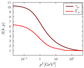
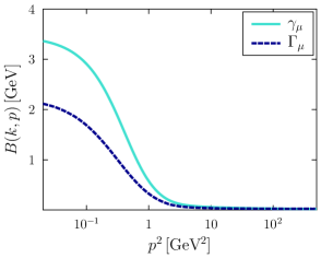
Figure 1: The quark-dressing functions $A(p,n)$ and $B(p,n)$ calculated with a bare vertex and with the WFGTI ansatz of Eq. (19).

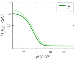
Figure 2: The quark-mass function $M(p,n)=B(p,n)/A(p,n)$ obtained with the bare and WFGTI vertices.

$$B(\mu,n)=m(\mu,n)=5\;\mathrm{MeV}\quad\text{and}\quad A(\mu,n)=1\ ,$$ (45)

at a renormalization scale $\mu=19$ GeV, whereas $C(k,n)$ is left unconstrained.

Likewise, we derive the integral equations (28) to (31) for the vertex in Eq. (19), the expressions of which we here omit due to their length.

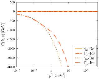
Figure 3: Real and imaginary parts of the dressing function $C(p,n)$ obtained with the RL and WFGTI vertices.

IV Gauge dependence of the quark propagator

We compare numerical solutions of the quark’s dressing functions for both, the vertex in Eq. (19) and the bare vertex, that is the solutions of Eqs. (38), (39) and (40) in the so-called rainbow approximation and their counterpart using the WFGTI-vertex. We first discuss the case of the bare vertex for which we choose $D\omega=(2.912\;\mathrm{GeV})^{3}$ and $\omega=0.4$ GeV in Eq. (37). The dressing functions $A(p,n)$ and $B(p,n)$ are presented in Fig. 1 from which we infer that their functional behavior is reminiscent of that found in covariant gauges Lessa:2022wqc . In Fig. 2 one observes the typical rapid increase of the mass function at a hadronic scale of about 1 GeV. Unlike the two other dressing functions $C(p,n)$ is complex valued, as illustrated in Fig. 3. The imaginary part of $C(p,n)$ tends to a finite small value at very low momenta and falls off rapidly after $p^{2}\gtrsim 1\;\mathrm{GeV}^{2}$, whereas the real part remains zero for all $p^{2}$ values. As we shall shortly see, we deal with a special case and the real part of $C(p,n)$ is generally non zero.

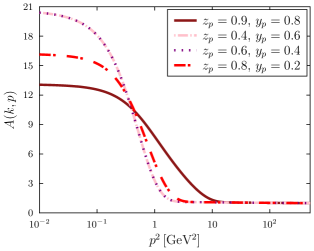
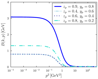
Figure 4: The gauge dependence of the scalar functions, $A(p,n)$ and $B(p,n)$, obtained with a bare quark-gluon vertex is due to the relative orientation of the vectors $n$ and $p$ and expressed by the angles $y_{p}$ and $z_{p}$ in Eq. (47).

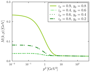
Figure 5: The dependence of the quark-mass function $M(p,n)=B(p,n)/A(p,n)$ on the orientation of the light-like vector $n$, see Eq. (47).

Turning to the case of the dressed vertex that satisfies the WFGTI (20), the integral equations for $A(p,n)$, $B(p,n)$ and $C(p,n)$ are more lengthy and the convergence of the numerical iterative procedure is considerably slower. So as to produce a constituent mass of comparable size than the one found with the RL truncation, we readjust the gluon interaction (37): $D\omega=(0.917\;\mathrm{GeV})^{3}$ and $\omega=0.4$ GeV. The wave renormalization and mass functions for this vertex are compared to the ones of the RL vertex in Fig. 1. Both, $A(p,n)$ and $B(p,n)$, are significantly suppressed in this case, yet the mass functions are qualitatively and quantitatively alike. Moreover, Fig. 3 shows that $C(p,n)$ is again a purely imaginary, monotonically decreasing function of $p^{2}$ which tends to a finite negative value in the small-momentum limit. It is worthwhile mentioning that for either vertex our results corroborate the analytic expression found in a one-loop calculation in light-cone gauge Mirja2020 , which shows that $C(p,n)$ is imaginary and decreases rapidly at large momenta.

As mentioned after Eqs. (34) and  (35), for either vertex we find the numerical solution $D(p,n,n^{*})=0$. The inverse of the quark propagator can therefore simply be written as:

$$S^{-1}(p,n)=A\,i\gamma\cdot p+B\,\mathbb{1}+C\,i\gamma\cdot n\,.$$ (46)

For convenience, the solutions presented in Figs. 1, 2 and 3 were obtained in the rest frame of the quark, $p=(\mathbf{0},|p|)$. In order to verify the dependence on the light-like vector $n=(0,0,1,i)$, we solve the DSE for an arbitrary momentum $p$, where the scalar product of both vectors is defined as,

$$n\cdot p=|p|\left(\sqrt{1-z_{p}^{2}}\,y_{p}+iz_{p}\right),$$ (47)

with angles $y_{p}=\cos\theta_{p}$ and $z_{p}=\cos\psi_{p}$. This allows us to investigate how the three dressing functions of the quark propagator explicitly depend on the relative orientation of the four-vectors $n$ and $p$. A rigorous calculation requires that $A(k,n)$, $B(k,n)$ and $C(k,n)$ in the kernels of Eqs. (38), (39) and (40) be functions of the three variables $p$, $y_{p}$ and $z_{p}$. Therefore, in solving iteratively this system of coupled integral equations, the values of $A(p,n)$, $B(p,n)$ and $C(p,n)$ must be obtained on a three-dimensional mesh for discrete values $p^{i}$, $y_{p}^{k}$ and $z_{p}^{l}$ in a first iteration and then fed back into the integral equations.

For simplicity’s sake, we here only consider the angular dependences of the explicit $n\cdot p$ terms in Eqs. (38), (39) and (40), and neglect it in the scalar functions which are simplify taken as: $A(k)$, $B(k)$ and $C(k)$. This suffices to reveal their dependence on the orientation of the light-like vector $n$. The behavior of the wave-renormalization and mass functions as functions of $y_{p}$ and $z_{p}$ in the RL-truncation is illustrated in Figs. 4 and 5 for a sample of representative angles. We observe a rapid increase of $A(p,k)$ and conversely an important suppression of $B(p,k)$ when the angles depart from their initial values $y_{p}=z_{p}=1\,\Rightarrow\,n\cdot p=i|p|$. Consequently, $M(p,k)$ is also suppressed. Note that with the present simplification of the integral equations, $A(p,n)$ and $B(p,n)$ are identical for pairs of angles, $y_{p},z_{p}$ and $y_{p}^{\prime}=z_{p},z_{p}^{\prime}=y_{p}$. Similarly, we note that for fixed values of $y_{p}$ these functions do not exhibit any variations but $C(p,n)$ rapidly falls off with increasing steepness as a function of $z_{p}$.

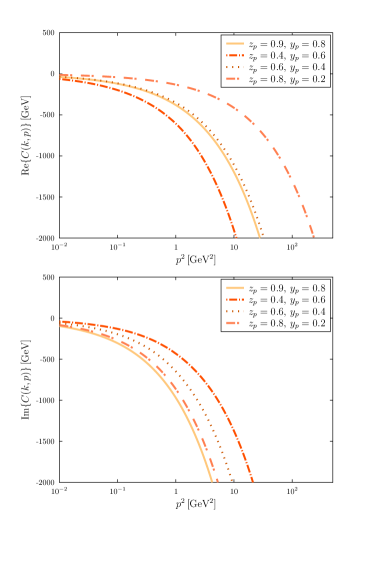
Figure 6: Angular gauge dependence of the real and imaginary parts of the dressing function $C(p,n)$ calculated with a bare vertex.

The $n$-dependent variation of the complex dressing function $C(p,n)$ for the same set of angles is depicted in Fig. 6. Clearly, when $y_{p}\neq 1$ and $z_{p}\neq 1$ the real part of $C(p,n)$ is non-zero for $p^{2}>0$ GeV² and its functional behavior mirrors the one of the imaginary part, decreasing rapidly with an $n$-dependent steepness for momenta larger than $|p|\gtrsim 1\;\mathrm{GeV}$.

V Concluding remarks

Motivated by phenomenological considerations, namely the intricacy of treating a Wilson line between two quark fields without resorting to expansions or simply neglecting the operator in the definition of distribution functions, we made a first step towards calculating the meson’s wave function in light-cone gauge. To that end, we have solved for the first time the DSE of a quark employing a model dressing function of the gluon propagator in light-cone gauge. We showed that the ML prescription is moot in solving the relevant DSE and that the dual vector $n^{*}$ is not needed.

As a consequence, the solutions of the nonperturbative quark propagator contain three scalar functions, two of them playing the usual role of the mass and wave-renormalization functions, while a third dressing function is complex. All three function depend on the relative orientation of the quark momentum $p$ and the light-like vector $n$. As such, the breaking of covariance in light-cone gauge is expressed by a geometric gauge dependence. The angular dependence of $A(p,n)$, $B(p,n)$ and $C(p,n)$ is found to be significant and in particular the mass function becomes suppressed when moving away from the quark’s rest frame. Naturally, a rigorous discussion of the quark gap equation in light-cone gauge requires the solution the gluon in the same DSE framework with its full dependence on the vector $n$, which may or may not compensate this suppression of the mass function.

Finally, since in light-cone gauge the gluon decouples from the ghost, we derive a dressed quark-gluon vertex that satisfies its WFGTI. With a readjustment of the gluon-dressing function we find that the dressing functions $A(p,n)$, $B(p,n)$ are suppressed in comparison with the same functions in the bare-vertex truncation of the DSE, nonetheless the resulting mass function is qualitatively and quantitatively equivalent. Since the convergence of the iterative procedure using Newton’s method is very slow in case of the WFGTI vertex for arbitrary values of $n\cdot p$, we refrained from studying the corresponding angular dependence of the dressing functions. Future improvements should implement the full angular dependence in the integral equations for $A(p,n)$, $B(p,n)$ and $C(p,n)$ and improve their numerical treatment.

With regard to the gauge independence of physical observables, only a symmetry preserving Bethe-Salpeter kernel for quark-antiquark states in the same light-cone gauge framework can offer a sensible path. This difficult task has been pursued in Landau gauge and should be seriously investigated in light-cone gauge in order to be able to calculate mesonic distribution amplitudes and parton distribution functions.

- (1) G. Leibbrandt, Rev. Mod. Phys. 59, 1067 (1987) doi:10.1103/RevModPhys.59.1067
- (2) A. C. Aguilar and J. Papavassiliou, JHEP 12, 012 (2006) doi:10.1088/1126-6708/2006/12/012
- (3) A. C. Aguilar, D. Binosi and J. Papavassiliou, Phys. Rev. D 78, 025010 (2008) doi:10.1103/PhysRevD.78.025010
- (4) C. S. R. Costa, A. Freese, I. C. Cloët, B. El-Bennich, G. Krein and P. C. Tandy, Phys. Rev. C 104, no.4, 045201 (2021) doi:10.1103/PhysRevC.104.045201
- (5) R. L. Jaffe, Contribution to: Ettore Majorana International School of Nucleon Structure: 1st Course: The Spin Structure of the Nucleon, 42-129 (1996) [arXiv:hep-ph/9602236 [hep-ph]].
- (6) F. E. Serna, R. C. da Silveira, J. J. Cobos-Martínez, B. El-Bennich and E. Rojas, Eur. Phys. J. C 80 (2020) no.10, 955 doi:10.1140/epjc/s10052-020-08517-3
- (7) F. E. Serna, R. C. da Silveira and B. El-Bennich, Phys. Rev. D 106 (2022) no.9, L091504 doi:10.1103/PhysRevD.106.L091504
- (8) L. Chang, I. C. Cloët, J. J. Cobos-Martínez, C. D. Roberts, S. M. Schmidt and P. C. Tandy, Phys. Rev. Lett. 110, no.13, 132001 (2013) doi:10.1103/PhysRevLett.110.132001
- (9) C. Shi, C. Chen, L. Chang, C. D. Roberts, S. M. Schmidt and H. S. Zong, Phys. Rev. D 92, 014035 (2015) doi:10.1103/PhysRevD.92.014035
- (10) C. Mezrag, H. Moutarde and J. Rodriguez-Quintero, Few Body Syst. 57, no.9, 729-772 (2016) doi:10.1007/s00601-016-1119-8 [arXiv:1602.07722 [nucl-th]].
- (11) C. Shi and I. C. Cloët, Phys. Rev. Lett. 122, no.8, 082301 (2019) doi:10.1103/PhysRevLett.122.082301 [arXiv:1806.04799 [nucl-th]].
- (12) F. E. Serna, B. El-Bennich and G. Krein, [arXiv:2409.01441 [hep-ph]].
- (13) J. R. Lessa, F. E. Serna, B. El-Bennich, A. Bashir and O. Oliveira, Phys. Rev. D 107, no.7, 074017 (2023) doi:10.1103/PhysRevD.107.074017
- (14) G. Leibbrandt, Phys. Rev. D 29, 1699 (1984) doi:10.1103/PhysRevD.29.1699
- (15) G. Leibbrandt, Nucl. Phys. B 310, 405-427 (1988) doi:10.1016/0550-3213(88)90156-3
- (16) S. Mandelstam, Nucl. Phys. B 213, 149-168 (1983) doi:10.1016/0550-3213(83)90179-7
- (17) G. Leibbrandt and S. L. Nyeo, Phys. Lett. B 140, 417-420 (1984) doi:10.1016/0370-2693(84)90783-4
- (18) Mirja Tevio, Quark mass renormalization in perturbative quantum chromodynamics in light-cone gauge, Master’s thesis, University of Jyväskylä (2020), http://urn.fi/URN:NBN:fi:jyu-202012117074
- (19) E. Newman and R. Penrose, J. Math. Phys. 3, 566-578 (1962) doi:10.1063/1.1724257
- (20) G. Leibbrandt, Phys. Rev. D 30, 2167 (1984) doi:10.1103/PhysRevD.30.2167
- (21) A. Bashir, L. Chang, I. C. Cloët, B. El-Bennich, Y. X. Liu, C. D. Roberts and P. C. Tandy, Commun. Theor. Phys. 58, 79-134 (2012) doi:10.1088/0253-6102/58/1/16
- (22) D. C. Curtis and M. R. Pennington, Phys. Rev. D 42, 4165-4169 (1990) doi:10.1103/PhysRevD.42.4165
- (23) C. S. Fischer and R. Alkofer, Phys. Rev. D 67, 094020 (2003) doi:10.1103/PhysRevD.67.094020
- (24) R. Alkofer, C. S. Fischer, F. J. Llanes-Estrada and K. Schwenzer, Annals Phys. 324, 106-172 (2009) doi:10.1016/j.aop.2008.07.001
- (25) A. Kızılersü and M. R. Pennington, Phys. Rev. D 79, 125020 (2009) doi:10.1103/PhysRevD.79.125020
- (26) R. Williams, Eur. Phys. J. A 51, no.5, 57 (2015) doi:10.1140/epja/i2015-15057-4
- (27) A. Bashir, A. Raya and S. Sanchez-Madrigal, Phys. Rev. D 84, 036013 (2011) doi:10.1103/PhysRevD.84.036013
- (28) A. Bashir, R. Bermúdez, L. Chang and C. D. Roberts, Phys. Rev. C 85, 045205 (2012) doi:10.1103/PhysRevC.85.045205
- (29) E. Rojas, J. P. B. C. de Melo, B. El-Bennich, O. Oliveira and T. Frederico, JHEP 10, 193 (2013) doi:10.1007/JHEP10(2013)193
- (30) E. Rojas, B. El-Bennich, J. P. B. C. De Melo and M. A. Paracha, Few Body Syst. 56, no.6-9, 639-644 (2015) doi:10.1007/s00601-015-1020-x
- (31) B. El-Bennich, G. Krein, E. Rojas and F. E. Serna, Few Body Syst. 57, no.10, 955-963 (2016) doi:10.1007/s00601-016-1133-x
- (32) D. Binosi, L. Chang, J. Papavassiliou, S. X. Qin and C. D. Roberts, Phys. Rev. D 95, no.3, 031501 (2017) doi:10.1103/PhysRevD.95.031501
- (33) R. Bermúdez, L. Albino, L. X. Gutiérrez-Guerrero, M. E. Tejeda-Yeomans and A. Bashir, Phys. Rev. D 95, no.3, 034041 (2017) doi:10.1103/PhysRevD.95.034041
- (34) F. E. Serna, C. Chen and B. El-Bennich, Phys. Rev. D 99, no.9, 094027 (2019) doi:10.1103/PhysRevD.99.094027
- (35) L. Albino, A. Bashir, L. X. G. Guerrero, B. E. Bennich and E. Rojas, Phys. Rev. D 100, no.5, 054028 (2019) doi:10.1103/PhysRevD.100.054028
- (36) L. Albino, A. Bashir, B. El-Bennich, E. Rojas, F. E. Serna and R. C. da Silveira, JHEP 11, 196 (2021) doi:10.1007/JHEP11(2021)196
- (37) B. El-Bennich, F. E. Serna, R. C. da Silveira, L. A. F. Rangel, A. Bashir and E. Rojas, Rev. Mex. Fis. Suppl. 3, no.3, 0308092 (2022) doi:10.31349/SuplRevMexFis.3.0308092
- (38) A. C. Aguilar and J. Papavassiliou, Phys. Rev. D 83, 014013 (2011) doi:10.1103/PhysRevD.83.014013
- (39) A. C. Aguilar, D. Binosi, D. Ibañez and J. Papavassiliou, Phys. Rev. D 90, no.6, 065027 (2014) doi:10.1103/PhysRevD.90.065027
- (40) A. C. Aguilar, M. N. Ferreira, G. T. Linhares, B. M. Oliveira and J. Papavassiliou, [arXiv:2408.15370 [hep-ph]].
- (41) J. C. Ward, Phys. Rev. 78, 182 (1950) doi:10.1103/PhysRev.78.182
- (42) E. S. Fradkin, Zh. Eksp. Teor. Fiz. 29, 258-261 (1955)
- (43) H. S. Green, Proc. Phys. Soc. A 66, 873-880 (1953) doi:10.1088/0370-1298/66/10/303
- (44) Y. Takahashi, Nuovo Cim. 6, 371 (1957) doi:10.1007/BF02832514
- (45) A. A. Slavnov, Theor. Math. Phys. 10, 99 (1972) [Teor. Mat. Fiz. 10, 153 (1972)]. doi:10.1007/BF01090719
- (46) J. C. Taylor, Nucl. Phys. B 33, 436 (1971) doi:10.1016/0550-3213(71)90297-5
- (47) B. Ma and C. R. Ji, Phys. Rev. D 104, no.3, 036004 (2021) doi:10.1103/PhysRevD.104.036004
- (48) G. Eichmann, E. Ferreira and A. Stadler, Phys. Rev. D 105, no.3, 034009 (2022) doi:10.1103/PhysRevD.105.034009
- (49) J. C. R. Bloch, Phys. Rev. D 66, 034032 (2002) doi:10.1103/PhysRevD.66.034032
- (50) P. Maris and P. C. Tandy, Phys. Rev. C 60 (1999), 055214 doi:10.1103/PhysRevC.60.055214