Exploring Galactic open clusters with Gaia

Abstract

Context. Mass is the most critical physical parameter in the evolution of a star. Since stars form in clusters their initial mass function (IMF) is decisive in their evolution.

Aims. Use Gaia DR3-based stellar masses mass_flame and the stellar members found for fifteen nearby open clusters from Paper I, to estimate their mass segregation and distribution.

Methods. For each cluster, the single stars’ main sequence was fitted with a moving straight line weighted fit to the Color-Magnitude Diagram, stars brighter than the residuals dispersion were taken as binaries. Single stars masses were obtained from a cubic spline fit to the mass_flame vs. $G$ magnitude data. For binary stars, the individual masses of each component were estimated using simulated-based inference. We used the minimum spanning tree concept to measure the mass segregation of each cluster. From the stellar mass distribution, an estimate of the power-law coefficient that best describes it was used to characterize the IMF.

Results. Mass segregation is visible in all the clusters, the older ones have $\sim$ 50% of their most massive stars segregated, while younger ones extend from $\sim$ 30% to $\sim$ 55%. The IMF of the studied clusters is well described by a power law of index $2.09\pm 0.23$.

Conclusions. Significant mass segregation, from one-third to one-half of its most massive population is present in open clusters as young as $\gtrsim$ 10 Myr. Mass segregation may be strong for only a few of the most massive stars or less intense but extended to a larger fraction of those, it may start as early as 0.20 of the relaxation time of the cluster and progress over time by increasing both the number of the most massive stars affected and their amount of segregation. Older open clusters show evidence of binary disruption as time progresses.

1 Introduction

The Initial Mass Function (IMF) stands as one of the fundamental pillars in the understanding of stellar populations and galactic evolution. First introduced by Salpeter (1955), who defined it as a power-law with the form $\xi(m)\propto m^{-2.35}$, the IMF describes the distribution of initial stellar masses formed in a star formation event, serving as a crucial input parameter for models of stellar evolution, chemical enrichment, and galaxy formation. This foundational concept has evolved significantly since its introduction. Miller & Scalo (1979) provided one of the first comprehensive analyses suggesting that the IMF might not follow a single power law across all masses. The theoretical framework supporting this suggestion was further developed through the multi-segment power-law proposed by Kroupa (2001), which introduces breaks at $0.08$, $0.5$ and $1$ $M_{\odot}$, and the log-normal distribution suggested by Chabrier (2003), which describes the observed mass distribution below $1$ $M_{\odot}$.

While these theoretical developments have been introduced to the IMF, observational challenges remain significant. Among the dynamical processes that shape open clusters, mass segregation —the tendency for more massive stars to concentrate toward the cluster center— emerges as a key phenomenon that influences both the spatial distribution of stars and the observed mass function. The advent of Gaia has revolutionized our understanding of these effects through unprecedented precision in stellar measurements and cluster membership determination. Notably, Tarricq et al. (2022), using Gaia EDR3 data of $389$ open clusters, found that older clusters tend to be more mass-segregated than younger ones, likely due to a combination of segregation and evaporation effects.

Recent studies have added understanding to the complex relation between cluster age and mass distribution. Pang et al. (2024) conducted a comprehensive analysis of the present-day mass function (PDMF) for 93 star clusters using Gaia DR3 data. They found that the power-law index ($\alpha$) of the PDMF remains stable at $\alpha\approx 2$ for clusters younger than $200$ Myr, consistent with the Kroupa (2001) IMF, but decreases significantly for older clusters, particularly when considering stars within the half-mass radius. This evolution of $\alpha$ with cluster age provides strong evidence for dynamical evolution effects, where low-mass stars are preferentially lost through processes like two-body relaxation and tidal stripping.

The theoretical understanding of these observational results has been refined by recent work. Hennebelle & Grudić (2024) provided a comprehensive review of the physical processes that determine the stellar IMF. They highlighted how the combination of gravity, turbulence, and feedback is responsible for establishing the high-mass power-law slope of the IMF. Depending on environmental conditions, the power-law index $\alpha_{\text{IMF}}$ can take values of $0$, $-0.8$, $-1$, or $-1.3$ (the Salpeter (1955) slope is $-1.35$, following the notation of this review). While these regimes may be universal, the stellar mass ranges where they apply depend on local conditions like magnetic field strength, Mach number, and temperature.

Building upon this theoretical and observational foundation, our work investigates both the IMF and mass segregation in a sample of $15$ open clusters. Our methodology combines established techniques with modern statistical analyses to: determine the present-day mass function and reconstruct the IMF while accounting for observational completeness limits and binary star effects; quantify the degree and spatial extent of mass segregation through multiple metrics and radial variation analysis; and examine the interplay between these phenomena and their implications for cluster evolution. Through this analysis, we aim to contribute to the ongoing discussion about the universality of the IMF and the role of mass segregation in shaping the observable properties of open clusters. Our work addresses key limitations of previous studies through improved methodology and comprehensive treatment of observational biases, building upon the theoretical framework established by these seminal works in the field.

This document is organized into six sections, summarized as follows. Section 2 presents the Gaia Astrophysical Parameters catalog, which aims to retrieve the stellar mass mass_flame for main sequence stars. It also details the selection of 15 open clusters with diverse ages and metallicities included in this study. Section 3 comprises four subsections: (i) identification and separation of binary stars from main sequence single stars, (ii) a brief overview of how cubic spline fitting was used to extrapolate stellar masses for single stars, (iii) estimation of mass for each component of the binary stars, and (iv) the application of the minimum spanning tree method to address the mass segregation problem. Section 4 presents the outcomes for each cluster regarding mass segregation and the initial mass function. Section 5 explores the advantages and limitations of the employed methodology, along with the implications and significance of our findings. Finally, we summarize our key conclusions and insights in Section 6.

2 Data

The lack of data due to observational limitations in the regime of low-mass stars is a real challenge in characterizing the IMF of star clusters. In the Gaia DR3 catalog, completeness down to $G\sim 21$ mag means it contains plenty of sub-solar stellar masses. Still, their astrometric and photometric errors are substantial enough to affect and bias estimates of physical parameters of interest, such as distance or mass per star, or the spatial distribution of a cluster of them. The catalog provided by Alfonso et al. (2024, hereafter Paper I) contains candidate member stars for 370 nearby open clusters using Gaia DR3 data, considering stars as faint as $G\sim 19.5$ mag (see Fig. 5 in Paper I). Their membership is robust and reaches faint enough stars to provide a good quality complete sample of low-mass coeval stars for which studying their IMF is suitable. A cross-match using Gaia source_id with Gaia DR3 Astrophysical Parameters catalog found that a total of $43,386$ stars have a measured mass_flame parameter.

The Astrophysical Parameters is an additional catalog to Gaia that contains information such as temperature, radius, mass, age, luminosity, stellar surface gravity and some chemical abundances. These parameters were computed based on BP/RP and RVS spectra, astrometry and photometry. Particularly, to produce a mass estimate for each star, the BaSTI stellar models (Hidalgo et al. 2018) and the atmospheric parameters ($T_{\text{eff}}$, log $g$, [$M/H$]) were combined for stars with $G<18.25$. The mass estimates come from the Final Luminosity Age Mass Estimator (FLAME), the method performs a Monte Carlo bootstrap to produce a sampling of each parameter. Then, it computes the estimated parameter as the $50_{\text{th}}$ percentile of the distribution and their lower and upper uncertainties as the $16_{\text{th}}$ and $84_{\text{th}}$ percentiles, respectively (see Section 11.3.6 in Gaia Collaboration et al. (2022) for details).

From the cross-match, we look for stars in the main sequence using the evolstage_flame $\leq 360$ flag. Every open cluster in Paper I have stars with masses reported in the astrophysical parameters. In the worst case, a cluster only has $5$ stars with masses, which is less than $10\%$ of its number of members. Therefore, we select clusters with at least $100$ stars with masses and a total of $64$ satisfy that condition. By visual inspection, we check their spatial distribution and select a final sample of $15$ open clusters to avoid those with high stretching in the line of sight due to biases in parallax (Bailer-Jones 2015; Luri et al. 2018). We note that the mass_flame reported errors sizes are almost always below $10\%$ of the estimated (median) mass.

3 Methods

In this section, we describe the methodology used on the collected stellar masses data to extend such estimates to all stars in the selected clusters, considering the special case of binary systems.

3.1 Identifying the binary stars with the sliding polynomial

The fifteen open clusters chosen visibly have binary stars. They can be seen in the G vs. BP$-$RP color-magnitude diagram (CMD) as a parallel brighter sequence from the main one. When the stars in the binary system have the same mass, the shift corresponds to $0.75$ magnitudes (Tauris & van den Heuvel 2023; Cordoni et al. 2023). To identify the main sequence single stars and separate them from the binary ones, we used a sliding polynomial function as proposed by Stock & Abad (1988). In this fitting procedure, a moving polynomial is fitted around any given point by considering only the data within a fixed interval, and the data closer to the point is given a larger weight. In our case, we fitted a straight line to the CMD values, with the color data weighted by

$$w_{i}=\left(1-\left(\frac{|C_{i}-C|}{dC}\right)^{2}\right)^{n/2}$$ (1)

with $dC$ being the window size around color C, $n$ an integer, and $C_{i}$ the $i$-th star’s color in the window. We use $n=3$ and $dC=0.5$ mag. Fig. 1 upper left panel shows the fit obtained for cluster Trumpler 10. The larger number of single stars and their concentration along the main sequence ties the sliding weighted straight line fit to it. The dispersion of the main sequence single stars at every color is well measured by 1.7 times the median absolute deviation of the residuals in its window and it is typically about $0.2$ magnitudes. We also included the condition of $G>8.5$ magnitudes to avoid classifying the subgiants and red giants as binary stars. Therefore, all stars brighter than this range are taken as binary stars. Fig. 1 lower left panel shows identified binary stars with colored symbols for Trumpler 10.

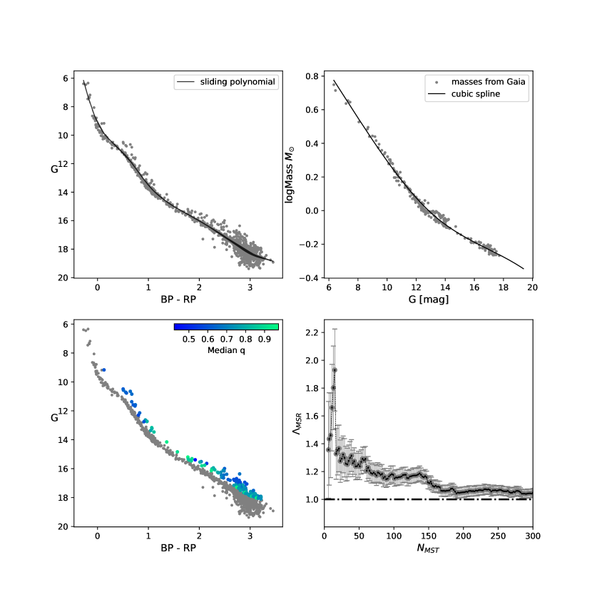
Figure 1: Results for the open cluster Trumpler 10 using the members provided in Alfonso et al. (2024). From left to right and top to bottom: CMD with the sliding polynomial to select binary stars, spline fitted to the masses in the Gaia Astrophysical Parameters catalog, CMD with the $q$ ratio computed through the SBI method, and the minimum spanning ratio ($\Lambda_{\text{MSR}}$) of the most massive stars to measure the mass segregation effect.

3.2 Mass estimates for single stars using splines

The collected mass_flame values from the Astrophysical Parameters catalog were used to produce mass estimates on stars lacking this parameter. To do so, we fitted a spline function on the known masses using the SciPy python library (Virtanen et al. 2020). A spline is a piece-wise polynomial function (De Boor 1978), commonly used for interpolating problems. Since it is defined using polynomials, the ones on the two extremes of the data points or knots can be formally extended beyond, therefore acting as an extrapolation, and probably close to the real function if it is not too far from the extreme knots. We used the spline function splrep in SciPy using a cubic polynomial. First, we fitted the spline on the logMass versus G magnitude relation with a smoothing condition of $s=0.1$. This condition controls the amount of smoothness in the sum of squared residuals, smaller values yield smoother fits. Then, the BSpline function in SciPy was used to perform extrapolation based on the tuple containing the vector of knots and the spline coefficients from splrep.

Fig. 1 upper right panel shows the spline fit (black line) obtained for Trumpler 10 to estimate the mass for each of the $929$ stars members found in Paper I, based on the $254$ ones with mass_flame values (gray points). These masses from Gaia reach down to $0.5$ $M_{\odot}$, while in the extrapolation process, they are extended down to about $0.3$ $M_{\odot}$ in the best cases.

Five of the fifteen open clusters have a few subgiants (SG) and red giants branch (RGB) stars. Alessi 9 has one SG or RGB with no mass_flame, NGC 2516 has five RGBs of which one has mass_flame, NGC 2632 has seven SGs of which six have mass_flame, NGC 3532 has six RGBs of which three have mass_flame, and NGC 6475 has one SG or RGB with no mass_flame. In the case of NGC 2632, their spline-based masses are very close to the Gaia mass_flame ones, but in other clusters some significant differences were found, with the spline-based mass being larger. In all these SG and RGB cases, the spline-based mass was used on the mass segregation calculations, since their order by mass is not altered significantly. On the other hand, for the IMF slope, these stars are omitted to avoid the bias their overestimated spline-based masses may introduce at the extreme right side of the IMF.

Table 1: IMF parameters for the target clusters.

Cluster	$N_{\text{stars}}$	$N_{\text{binaries}}$	$\alpha$	$m_{\text{total}}$	$m_{\text{lower}}$	$m_{\text{upper}}$	Age${}_{\text{*}}$	Age${}_{\text{CG}}$
				$M_{\odot}$			Myr
Pozzo 1	626	79	$2.30^{+0.17}_{-0.23}$	472.9	$0.48$	$5.46$	11.6	9.5
NGC 2547	465	63	$2.08^{+0.30}_{-0.24}$	387.4	$0.45$	$3.15$	27.6	32.4
IC 2602	462	60	$1.89^{+0.28}_{-0.26}$	325.4	$0.37$	$2.68$	33.1	36.3
Trumpler 10	929	116	$2.22^{+0.05}_{-0.07}$	767.4	$0.48$	$3.59$	40.1	32.4
BH 99	544	64	$2.15^{+0.06}_{-0.06}$	450.4	$0.44$	$3.38$	45.5	95.5
Alessi 5	340	38	$1.92^{+0.28}_{-0.33}$	294.1	$0.45$	$3.76$	48.9	67.6
NGC 7058	313	44	$2.51^{+0.42}_{-0.53}$	205.5	$0.30$	$2.26$	78.8	40.7
Blanco 1	579	68	$2.13^{+0.20}_{-0.24}$	336.0	$0.29$	$1.75$	79.5	104.7
Melotte 22	1130	98	$2.05^{+0.09}_{-0.10}$	723.3	$0.30$	$2.56$	103.5	77.6
NGC 6475	1091	106	$1.88^{+0.24}_{-0.15}$	1009.3	$0.41$	$3.46$	271.0	223.9
ASCC 101	154	17	$1.90^{+0.25}_{-0.42}$	131.7	$0.39$	$3.32$	276.7	489.8
Alessi 9	267	28	$1.78^{+0.07}_{-0.08}$	199.1	$0.32$	$2.65$	302.4	281.8
NGC 3532	2206	249	$1.74^{+0.26}_{-0.36}$	2052.0	$0.39$	$2.91$	651.6	398.1
NGC 2516	2520	261	$2.29^{+0.14}_{-0.12}$	1998.9	$0.39$	$4.75$	674.8	239.9
NGC 2632	862	78	$2.45^{+0.16}_{-0.17}$	565.6	$0.42$	$1.69$	946.3	676.1

3.3 Individual masses of binary stars components derived from simulation-based inference

While all single stars in each cluster have estimated masses from the spline fit, for the identified binary stars we compute the corresponding (or most probable) individual masses for each member of the binary system. We used a Simulated-Based Inference (SBI) method (Cranmer et al. 2020), also known as likelihood-free inference, proposed by Wallace (2024) with photometry from Gaia, Two Micron All Sky Survey (2MASS) and Wide-field Infrared Survey Explorer (WISE) catalogs. The method is based on computing the astrophysical parameters $M_{1}$, $q$, age, $[\text{Fe}/\text{H}]$, and distance from the observed photometry. To do so, the SBI approach aims to approximate the posterior distribution of the astrophysical parameters with no assumptions about the form of the likelihood function for a given data. Overall, SBI works by using a set of parameters to generate mock data and training a neural network to determine a relation between the parameters and data (see Wallace 2024, for a detailed description).

We follow the same methodology applied by Wallace (2024), in which a training set of $100000$ stars is simulated with the isochrones package (Morton 2015) to feed the model. Then, the SBI method produces an approximate posterior distribution of the parameters per star, thus we can obtain the most probable parameters of the distributions as those inferred. Once the model is trained, we feed it with the Gaia photometry of the binary stars per cluster. Fig. 1 lower left panel shows the distribution of the inferred $q=M_{2}/M_{1}$ ratio from the SBI method for the Trumpler 10 open cluster. As noted by Wallace (2024), a true binary is considered only when $q\geq 0.5$, below this threshold, it is unlikely that the binary system might be cleanly resolved by photometry since their excess brightness above the main sequence is within the observed photometry dispersion. We consider a star as binary if $q\geq 0.5$, below this threshold the spline-based mass remains unchanged. Then, as the method produces an estimate on $M_{1}$, we obtain the secondary mass as $M_{2}=qM_{1}$.

The method is mostly sensitive to yielding low $q$ ratios for stars above the main sequence at the low-mass regime. This bias may be due to high astrometric errors when approaching to the faintest limit as noted by Rybizki et al. (2022) and Paper I. In addition to this, Wallace (2024) also claimed that the method is fully sensitive to the priors used, mainly on age and metallicity. This require further research and a detail examination, which is out of the scope of this work. However, despite that the model is less sensitive at recovering binary fractions in the faintest limit, we take them as such if they fulfill the requirement of $q\geq 0.5$. Each binary spline-based mass is finally substituted by two masses, $M_{1}$ and $M_{2}$. Therefore the total number of stars per cluster, accounting for the two components of each binary stars is given by $N_{\text{stars}}+N_{\text{binaries}}$ listed in Table 1. All calculations on mass segregation and IMF considered this total number of stars per cluster. On the other hand, the calculation of the percentage of binary stars is given by $N_{\text{binaries}}/N_{\text{stars}}\times 100\%$.

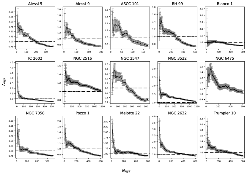
Figure 2: Mass segregation results. $\Lambda_{MSR}$ vs. $N_{MST}$ for the fifteen open clusters studied in this paper. No mass segregation is marked by the horizontal line $\Lambda_{MSR}=1.0$. The vertical error bars correspond to the $\sigma_{\text{random}}$ computed at each $N_{MST}$.

3.4 Mass segregation using the minimum spanning tree

The Minimum Spanning Tree (MST) of a distribution of points consist of a path connecting all points with the shortest possible path-length with no closed loops (Wu & Chao 2004). The MST has been widely used to detect the mass segregation effect in star clusters, by comparing the length of massive stars’ MST to the one of randomly selected stars. In order to quantifying the mass segregation effect, we follow the methodology described by Allison et al. (2009). This method constructs the MST of the $N$ most massive stars ($N_{MST}$) and compares it to the MST of several samples of $N_{MST}$ random stars. For a cluster with mass segregation, it is expected that the length of the $N$ most massive stars is shorter than the average length of the $N$ random stars. On the other hand, if the length of the $N$ most massive stars is greater than the average length of $N$ random stars, the cluster exhibits inverse mass segregation. A cluster with non-segregation thus contains a similar length of the MST for the massive stars and the random sample.

The quantification of the mass segregation using the MST proceeds as follows:

• Sorts the data in descending order according to the mass of the stars. Then, compute the length of the $N_{MST}$ most massive stars ($l_{\text{massive}}$).

• Compute the average length and dispersion of a set of $N_{MST}$ random stars $\left\langle l_{\text{random}}\right\rangle\pm\sigma_{\text{random}}$ (assuming a Gaussian dispersion).

• Determine the mass segregation ratio ($\Lambda_{MSR}$) and its uncertainty as

  $$\Lambda_{MSR}=\frac{\left\langle l_{\text{random}}\right\rangle}{l_{\text{massive}}}\pm\frac{\sigma_{\text{random}}}{l_{\text{massive}}}$$ (2)

• Repeat the previous steps for different values of $N_{MST}$. Finally, plot $\Lambda_{MSR}$ versus $N_{MST}$ to observe the level of mass segregation in the cluster.

The number of times to capture random stars is not arbitrary. Numerical experiments have shown that using $50$ or more random sets is advisable for good estimates of errors (Allison et al. 2009). In this work we found that $300$ random sets yielded quite stable values of $\left\langle l_{\text{random}}\right\rangle$. We compute the MST on the Galactic cartesian coordinates $X$, $Y$ and $Z$, using the MiSTree Python package (Naidoo 2019) with the Kruskal’s algorithm (Kruskal 1956). Fig. 1 lower right panel shows the $\Lambda_{MSR}$ vs $N_{MST}$ for Trumpler 10. In this cluster the highest signature of mass segregation is observed among the 20 most massive stars with $1.4\lesssim\Lambda_{MSR}\lesssim 1.9$, which then drops abruptly to $\Lambda_{MSR}\approx 1.3$ for $20<N_{MST}<70$. However, the segregation signature is still larger than 1.0 within the error bar for down to the 170 most massive stars in Trumpler 10. These results are discussed in the following section.

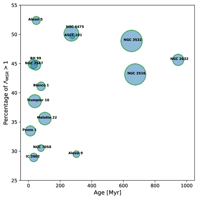
Figure 3: Percentage of the most massive stars with mass segregation vs. age, for each of the fifteen open clusters studied. The size of the circle is a measure of the total estimated mass of each cluster.

4 Results

4.1 Mass Segregation

The results of mass segregation obtained by this investigation for all the open clusters are shown in Fig. 2. A qualitative analysis of the observed plots shows that some clusters have a smooth decline in $\Lambda_{MSR}$ vs $N_{MST}$ (Alessi 5, IC 2602, and NGC 2632), while others have a significant drop from a higher value of $\Lambda_{MSR}$ to a lower more or less flat value (Blanco 1, NGC 3532, NGC 7058, Pozzo 1, and Melotte 22). Interestingly, an important number of the clusters show less mass segregation among the first most massive stars, which increases for less massive stars, and later decreases for larger values of $N_{MST}$. For some clusters, this shift in the maximum value of mass segregation occurs among a few of the most massive stars (Alessi 9, ASCC 101, BH 99, NGC 2516, and Trumpler 10), but for NGC 2547 and NGC 6475 it extends significantly in mass. In each of the above three descriptions of $\Lambda_{MSR}$ vs $N_{MST}$, we did not find any age trend, meaning in each of them we found clusters of various ages.

As for the measured amount of mass segregation, we found that NGC 2632 - also the oldest in our sample (see Table 1) - reaches values of $\Lambda_{MSR}\approx 3$, more specifically its $10$ most massive stars minimum spanning tree is about three times smaller than that of the average random set of stars of the same size. Cluster IC 2602 reaches an even higher $\Lambda_{MSR}\approx 3.5$ for the $N_{MST}=6$, but immediately drops to $\Lambda_{MSR}\approx 2.0$, which may be simply the result of small number statistics. Most of the clusters studied show their highest values of mass segregation in the range $1.2\lesssim\Lambda_{MSR}\lesssim 1.4$, and a few reach values of 2.0 (Alessi 5, Melotte 22 and NGC 7058).

We also studied for each cluster, the percentage of the most massive stars that exhibit mass segregation (the largest $N_{MST}$ for which $\Lambda_{MSR}>1$ divided by the total number of stars counted in the cluster (accounting for the two components of each binary) vs. their estimated age from Paper I. Results are plotted in Fig. 3. Our clusters’ ages roughly range in $10-950$ Myrs old, and our results show that the older open clusters have a large percentage ($\sim$ 50%) of their most massive stars segregated, notably also including the most populated massive clusters. On the other hand, in younger clusters, this percentage varies more extensively from $\sim$ 28% to $\sim$ 55%.

4.2 Initial Mass Function (IMF)

The open clusters studied in this investigation are all younger than 1 Gyr, half of them younger than 100 Myr, and a third of them - all older than 250 Myr - having only a few SGs, RGBs or WDs (Alessi 9, Melotte 22, NGC 2516, NGC 2632, NGC 3532, and NGC 6475). We did not see any significant difference in the mass distribution slope with age, and all the younger clusters only have main sequence stars, therefore we conclude the obtained mass distribution is a truthful representation of the IMF of these clusters.

To construct the IMF for each open cluster, we count the number of stars in six bins of equal width in $\log$ Mass between the lowest and highest individual stellar mass of each cluster. The number of stars is plotted with a blue triangle on the lowest extreme of each mass bin. The IMF is fitted by a power-law function given by

$$\xi(m)=Am^{-\alpha}dm,$$ (3)

where $A$ is a normalization constant, $\alpha$ is the power-law index, and $\xi(m)$ is the number of stars in the range $(m,m+dm)$. For this fitting, we use only the bins located from the mode onwards, as shown in Fig. 4. The case of the power-law index $\alpha=2.35$ is referred to as the well-known Salpeter (1955) slope. To fit Eq. (3) we use the Maximum Likelihood Estimation and a Markov chain Monte-Carlo (MCMC) approach. First, we produce the likelihood function for the sample of $N$ masses per cluster as the product of the individual probabilities associated with each mass $m_{i}$ (see Pang et al. (2024) for details):

$$\mathcal{L}=\prod^{N}_{i=1}p(m_{i}|A,\alpha)=\prod^{N}_{i=1}\xi(m_{i},A,\alpha)$$ (4)

From Eq. (4) we can obtain the log-likelihood function:

$$\log\mathcal{L}=\log A-\alpha\sum^{N}_{i=1}\log m_{i},$$ (5)

where the model parameters are the normalization constant $A$ and the power-law index $\alpha$. Then, to look for the set of parameters that maximize the log-likelihood function (5), we used the minimize method in SciPy (Virtanen et al. 2020) to minimize the negative of the log-likelihood function performing the Nelder-Mead algorithm. Second, to estimate uncertainties on these parameters, we implement an MCMC sampling using the emcee Python package (Foreman-Mackey et al. 2013). The sampling was performed with one hundred random walkers and two thousand iterations. Uniform priors on the model parameters were used, and the lower and upper uncertainties were chosen as the $16_{\text{th}}$ and $84_{\text{th}}$ percentiles. We validate the convergence of the chains by looking the Gelman & Rubin (1992) diagnostic $\hat{R}$, in which the variance between the chains and the variance in the chains are compared. We confirm that for all clusters, values of $\hat{R}\leq 1.2$ were obtained, indicating that the convergences have been reached.

Table 1 shows the IMF power-law index with its estimated uncertainties, for the fifteen open clusters. Fig. 4 depicts their IMFs and the fitted power-laws, blue triangles and lines represent the IMF. The estimated individual masses of the binary stars components (see Section 3.3) were used. The IMF mean slope for the studied open clusters is $-2.09\pm 0.23$.

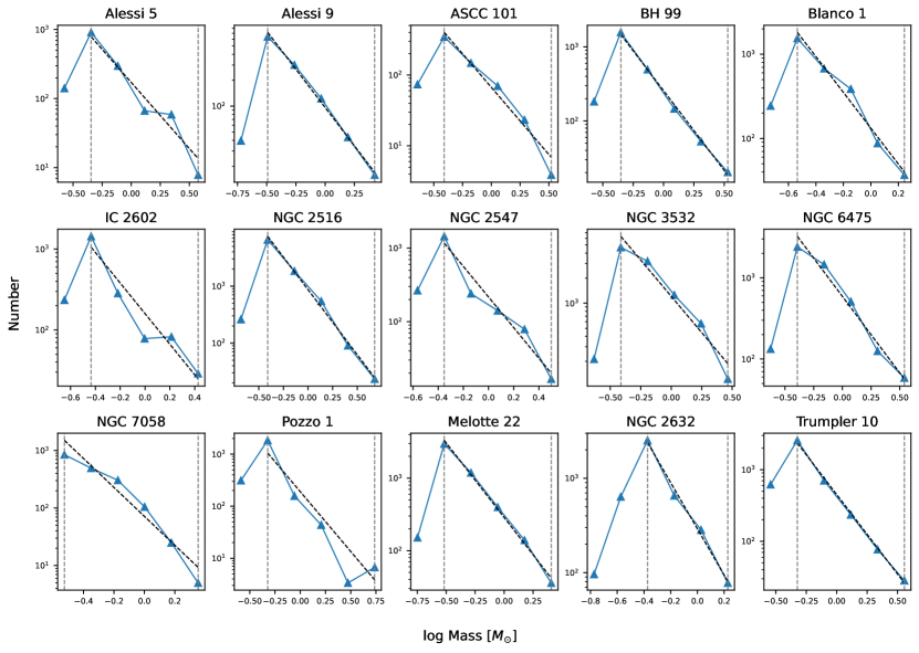
Figure 4: IMF of the fifteen open clusters. Blue lines represent the IMF using the masses estimated for all stars, single and binaries. The black dashed line is the power-law fit to the blue triangles, from the mode of the IMF marked by a vertical gray dashed line onwards.

5 Discussion

The first point to discuss is the estimated masses of binary stars computed in this investigation. The isochrones employed to assess the masses of the stars by the SBI treatment (Cranmer et al. 2020) are not the same as the ones used by Gaia (Hidalgo et al. 2018, BaSTI). This is not ideal but it is a good enough first approach. In any case, there is room for improvement, since we already have robust estimates of distance, age, and metallicity for each star from Paper I, consequently, we only need inferences on M1 and q. We are working on an improved procedure considering these priors for our next investigation.

On the other hand, uncertainties impose hard limits on what can be truly improved in this case. To evaluate this, we considered two other treatments for the individual masses of the binary star components. First, we considered the binary stars as single and used their spline-based mass, and second, we entirely omitted the binary stars. The results obtained in both cases were not drastically different from the ones presented here.

By taking a binary star as a single one, we count two lower-mass stars as one of higher mass. In other words, we are missing two stars of lower mass and adding one of higher mass. On the other option, i.e., ignoring the binary star from the mass distribution altogether, we are missing two stars of lower mass. In both cases, the effect is to make the IMF slope steeper, i.e. more negative than it is. Since our identified binaries amount only to 10%$-$15% of all the members $N_{\text{stars}}$ of the cluster, when ignoring the binaries we are reducing the total number of stars by at most twice this factor, mainly at lower mass values. The first procedure looks less harmful. If such biased and forceful treatments did not visibly alter the results, then our current more sophisticated approach must not be far from true, uncertainties permitting.

A second consideration is what coordinates $X$, $Y$ and $Z$ are assigned to the secondary stars in the binary systems. After the binary correction using the SBI approach in Sect. 3.3, the new estimated masses require Galactic cartesian coordinates to be included in the process of computing the MST. Conversely, identifying the possible positions of the two components requires additional information, such as the system’s period, and in our case, we only have their masses. However, the separation of binary stars does not exceed $3000$ AU (Jerabkova et al. 2019) even in the case of wide binaries, which are rare in open clusters (Deacon & Kraus 2020). For the closest cluster in our study, Melotte 22, this difference translates into a maximum parallax deviation for the secondary of less than one microarcsecond with the primary’s parallax, clearly below the parallaxes uncertainties in the Gaia data. In any case, assigning the same position to both binary components - as we do - does not affect the calculation of the MST for the mass segregation effect.

Pera et al. (2022) found a trend of $\Lambda_{MSR}\sim 1.4$ for the $10$ most massive stars in NGC 2516, which agrees with our results. By comparing the cluster age and its relaxation time, they conclude that this segregation is primordial rather than a dynamical effect. However, the age taken by Pera et al. (2022) (100 Myr old) is much younger than the one used in Paper I and that of Cantat-Gaudin et al. (2020). The open cluster Blanco 1 was also studied by Zhang et al. (2020), in which a mass segregation was found for members more massive than $1.4$ $M_{\odot}$ with $\Lambda_{MSR}\sim 1.5$, this result is in agreement with a $\Lambda_{MSR}\sim 2.5$ for the first $9$ massive stars found in this work. The segregation of the $20$ most massive stars in the Pleiades, with $\Lambda_{MSR}\sim 2.0$, is in agreement with the result of Raboud & Mermilliod (1998) and Converse & Stahler (2008). In addition, Heyl et al. (2022) found a skewed distribution of low-mass stars in the Pleiades (Melotte 22) by looking for escape stars beyond its tidal radius, which is expected from mass segregation in the cluster, however, despite that Heyl et al. (2022) did not compute the MST, the segregation is still evident if looking the evolution of escape stars as a function of time (see Fig. 9 in Heyl et al. (2022)). Overall, the complex dynamical evolution of open clusters is far from straightforward, for instance, Dib et al. (2018) obtained a skewed distribution of mean $\Lambda_{MSR}$ considering only $N_{MST}\leq 10$ for $1276$ Galactic clusters, in which $180$ clusters were found segregated with $\Lambda_{MSR}>1.5$ indicating mass segregation in all of them. For 13 out of our 15 clusters (missing only BH 99 and Pozzo 1), Dib et al. (2018) found the abovementioned mean value of $\Lambda_{MSR}$ to be larger than $1.0$, which is consistent with our results.

The typical timescale for dynamical mass segregation driven by two-body interactions is the relaxation time $t_{\text{relax}}$, which for a stellar cluster depends on the number of member stars and its crossing time $t_{\text{cross}}$, as follows from Binney & Tremaine (2008):

$$t_{\text{relax}}=\frac{N_{\text{stars}}}{8\ln{N_{\text{stars}}}}t_{\text{cross}}\,,$$ (6)

with $t_{\text{cross}}$ estimated from the diameter divided by a typical velocity dispersion taken as $1$ km/s, or equivalently $1.023$ pc/Myr. Alfonso & García-Varela (2023) measured the tidal radius of Blanco 1, Melotte 22, and NGC 2632, as $13.97$, $11.35$, and $12.12$ pc, respectively. Considering the number of stars $N_{\text{stars}}$ found for these clusters in Paper I, and taking twice the tidal radius as the diameter of the cluster, the estimated relaxation times of these clusters are $311$, $446$, and $378$ Myr, respectively (rounding to the closest integer). As a result, Blanco 1 and Melotte 22 have lived only $0.25$ of their relaxation time but NGC 2632 has already lived $2.5$ times its $t_{\text{relax}}$. From Fig. 2, we can see the progression of mass segregation from Blanco 1 ($79.5$ Myr old), to Melotte 22 ($103.5$ Myr old), to NGC 2632 ($946.3$ Myr old), in both the number of the most massive stars being the most segregated and the amount of their segregation.

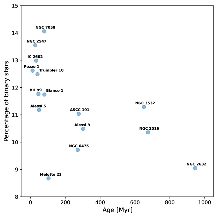
Figure 5: Percentage of binary stars computed as $N_{\text{binaries}}/N_{\text{stars}}\times 100\%$ vs. age, for each of the fifteen open clusters studied.

Interestingly, very young clusters like NGC 3603 - estimated to be 1-3 Myr old - exhibit mass segregation (Stolte et al. 2006; McMillan et al. 2007). An alternative explanation for these cases has been proposed by, e.g., McMillan et al. (2007), this mass segregation is primordial, more precisely inherited, the cluster is the result of mergers of small clumps that are initially mass segregated by two-body relaxation before they merge. Our results in Fig. 3 show that some of our youngest (age $\lesssim$ 100 Myr) open clusters show a significant portion of their population segregated by mass. Moreover, the youngest cluster in our sample - 11.6 Myr old Pozzo - has about 34% of its most massive stars segregated, and the cluster with the largest portion of stars mass-segregated - with 52% of its most massive stars segregated, is 48.9 Myr old Alessi 5. But these cases may illustrate different degrees of progress and success of dynamical mass segregation over the scale of tens of million years, not being young enough to prove the primordial mass segregation scenario.

The effects of two-body collisions over time on binary stars are also worthy of consideration. Three generally recognized mechanisms break binaries apart: (i) supernova explosion of one of the stars, (ii) close interactions with other stars, and (iii) wide binaries unbinding (Binney & Tremaine 2008; Ciotti 2021). The same two-body collisions that cause mass segregation among single stars do cause binary stars disruption (Vesperini et al. 2011; Bromley et al. 2012). What outcome arises first - mass segregation or disruption - is hard to ascertain, but we see the percentage of binary stars - $N_{\text{binaries}}/N_{\text{stars}}\times 100\%$ from Table 1 - being lower for the older clusters (see Fig. 5). The difference between the cluster with the largest proportion of binary stars, 78.8 Myr old NGC 7058 with 14% binary stars, versus the one with the least binary stars, 946.3 Myr old NGC 2632 with 9% of binary stars, also the oldest cluster in our sample, is only 5%. More clusters need to be studied to give statistical robustness to this result. But it points to the fact that older clusters would have fewer binary stars, due to their being disrupted over time.

In a cluster old enough, dynamical mass segregation will occur regardless of the initial state of mass segregation. The longer dynamical mass segregation is acting the more effective it will segregate the most massive stars and its effect is also faster on the more massive stars (Portegies Zwart et al. 2010). In our sample, clusters IC 2602 ($33.1$ Myr) and NGC 2632 ($946.3$ Myr) both reach a high $\Lambda_{MSR}$ (see Fig. 2), meaning their most massive stars are much closer than in other clusters. Nonetheless, in the younger cluster, those heavily concentrated most massive stars represent a much smaller percentage of the total number of stars than in the older cluster (see Fig. 3). Both clusters have similar total masses but IC2602 has a higher top current mass (see Fig. 4). We conclude that IC 2602 shows the faster mass segregation acting on the more massive stars in a shorter time, while in NGC 2632 we see mostly the effect of dynamical mass segregation on an extended period. It can not be ignored that NGC 2632 has a few white dwarfs (WD) (12 out of 940 stars, binaries included), for which our estimated masses are not only incorrect but more importantly, in the past they were the most massive stars in the cluster. Estimating their current mass is beyond the scope of this paper. Nonetheless, we visually inspected their current distribution in each of the XYZ coordinates and compared them to the whole cluster and the 35 most massive stars subset, and NGC 2632’s WDs look like the cluster, therefore we can speculate that after becoming white dwarfs very early in the history of NGC 2632, dynamical mass segregation has acted on them with their current lower mass, by pushing them away as time passes, then reversing their original concentration when they were massive stars. In any case, measuring their initial mass segregation status is impossible because two-body relaxation has - by definition - erased the previous dynamics and therefore positions.

Several other clusters of different ages have a large percentage of their segregated stars doing so but at lower values of $\Lambda_{MSR}\approx 1.4-2.0$. What makes dynamical segregation more intense on the few most massive stars or less intense but affecting a larger proportion of such stars, may depend on many factors, including the number of stars in the cluster, the total mass of the cluster, and how massive is the highest mass of the cluster.

A final comment on these results is that the selected sample of fifteen clusters out of 370 available from Paper I, was chosen for looking not too stretched in 3D space, due to Gaia parallax uncertainties. Theoretically, the MST approach to mass segregation could overcome this effect and still be able to measure segregation if present, despite the obvious deformation in the shape of the cluster. Here, we have tested MST works in the more nominal-looking ones. The trends found with age may be the result of the limited sample used, but overall, our findings do not contradict what is qualitatively expected for both mass segregation and binary star population evolution with age.

Regarding our results on the IMF slope, since we followed the same method of Pang et al. (2024), we compare our $\alpha$ from Table 1 with their $\alpha_{\text{PDMF}}$ in their Table 1. Only ten clusters are in common between both studies and for these, Pang et al. (2024) yield a mean power-law index of $1.90\pm 0.23$. For the same ten clusters, we obtain $2.05\pm 0.22$. The above values are within the error bars of the result for all fifteen open clusters, which is $2.09\pm 0.23$.

A recent review on the physical origin of the IMF by Hennebelle & Grudić (2024) summarizes how different mechanisms can yield primordial variations of the IMF, particularly below 0.5 M_⊙, where the slope could reduce to zero and even become positive below 0.2 M_⊙ (see their Fig. 3). Regarding the possibility that our clusters’ IMF may not be truly characterized by a single power law fit but rather a piecewise function, particularly at the low mass regime, our results in Fig. 4, show some slight variations that could be or not significant, given the size of our sample. We see some variations in the IMF slope particularly between 0.3 $-$ 1.0 M_⊙ for some of the clusters. Three of the older clusters (NGC 6475, ASCC 101, and NGC 3532) have a smaller slope but also does one young cluster (NGC 7058). On the other hand, four of the younger clusters (Pozzo 1, NGC 2547, IC 1602, and Alessi 5) have a higher slope than the overall power law index fit.

Considering the binary stars’ contribution when adding the secondary star mass will increase the observed slope, and indeed three of the above-mentioned younger clusters are at the higher end of the percentage of binary stars in Fig. 5. On the other hand, if mass segregation has been strong enough to eject low-mass members, including disrupted binary stars secondary masses when acting over time, the slope can be reduced. All of the above-mentioned older clusters have a lower percentage of binary stars. Separating the effect of sustained mass segregation from primordial variations of the IMF slope is complicated by the uncertain age estimations against which to compare their relaxation time.

5.1 Revision of cluster ages from previous literature

All the previous discussion is based on the ages of the open clusters as estimated by Paper I. In our previous investigation, we noticed a trend between our ages log(age)${}_{\text{Paper I}}$ and those of Cantat-Gaudin et al. (2020) log(age)${}_{\text{CG}}$, for older clusters (see Fig. 9 upper panel in Paper I). More specifically, we noted that $\Delta$log(age) $=$ log(age)${}_{\text{Paper I}}$ - log(age)${}_{\text{CG}}$ vs log(age)${}_{\text{Paper I}}$ becomes positive and reaches up to 0.5, for log(age)${}_{\text{Paper I}}\gtrsim 8.2$, i.e., age $\gtrsim$ 160 Myr.

For this reason, we also explored the trends we observed in the percentages of mass segregation and binary stars with age, as seen in Figs. 3 and 5 respectively, using the ages log(age)${}_{\text{CG}}$, listed also in Table 1. The corresponding two plots can be seen in Fig. 6 in the Appendix A. The percentage of mass segregation trend with age remains but does not longer correlate with mass as Fig. 3 suggested, therefore, we conclude that it is higher for older clusters, regardless of the total mass of the cluster. Regarding the progression of mass segregation with age by checking the behavior of $\Lambda_{MSR}$ against how many relaxation times the cluster has lived, considering Cantat-Gaudin et al. (2020)’s ages change age$/t_{\text{relax}}$ for Melotte 22 (age${}_{\text{CG}}=77.6$ Myr) and Blanco 1 (age${}_{\text{CG}}=104.7$ Myr), both from 0.25 to 0.17 and 0.34, respectively. For NGC 2632, this factor changes from 2.5 to 1.79 (age${}_{\text{CG}}=676.1$ Myr). In all cases, our conclusion remains valid, we can see the progression of mass segregation from younger to older clusters in both the number of the most massive stars being the most segregated and the amount of their segregation, considering their relaxation time. As for how early mass segregation may start, we resorted to using an average age from Paper I and Cantat-Gaudin et al. (2020), which casually are about the same, $\sim$ 90 Myr old, for both. Considering these average ages, mass segregation may start as early as 0.20 $t_{\text{relax}}$. As for the percentage of binary stars vs age, our conclusion remains the same, their proportion against the total number of stars in the clusters diminishes with time.

Another important note in this regard refers to the $m_{\text{upper}}$ values listed in Table 1 vs age. As it is well established that older clusters have lower-mass turn-off points, the expected trend should be that older clusters have lower $m_{\text{upper}}$ values. Cluster NGC 2516 stands out for having a high $m_{\text{upper}}$ for what was estimated to be a somewhat old cluster by Paper I, but its log(age)${}_{\text{CG}}$ is significantly younger, which is more consistent with what we obtained from its main sequence spline-based masses. We checked that for this cluster, the Gaia Astrophysical Parameters catalog has a main sequence bright star, source_id=5289522090708710656, with mass_flame=7.1672807 Msun, that also has parameters calculated by the Extended Stellar Parametrizer for Hot Stars (ESP-HS) routine, which lists a spectral type spectraltype_esphs=B for it. Keep in mind that $m_{\text{upper}}$ marks the lower extreme of the mass bin used in the IMF plot, and it contains this star in the calculation because it is taken as a main-sequence star from its value of evolvstage_flame=267.

This apparent drawback gives support to the spline-based masses employed in this investigation and points us to a potential procedure to revise the open cluster ages from Paper I and other references, using the Gaia Astrophysical Parameters catalog and the mass distributions. In this way, the highest main sequence star spline-based mass based on mass_flame must correlate with the estimated age, as expected from well-established results of stellar evolution. This insight will be considered for future investigations.

6 Conclusions

Below, we highlight the overall conclusions of this work:

• Mass segregation is visible in all the clusters, the older ones have a large percentage ($\sim$ 50%) of their most massive stars segregated, while younger ones have more varied values, the least being $\sim$ 30%.

• Significant mass segregation of a third or more of its population is present in open clusters as young as 10 $-$ 100 Myr.

• Mass segregation may be strong for only a few of the most massive stars or less intense but extended to a larger fraction of those stars.

• Mass segregation may start as early as $0.20$ of the estimated relaxation time of a cluster.

• Dynamical mass segregation progresses over time by increasing the number of the most massive stars being the most segregated and the amount of their segregation.

• Older open clusters show evidence of binary disruption as time progresses.

• The IMF of the selected nearby fifteen open clusters, which goes below $M_{\odot}=0.4$ in eight out of fifteen clusters, is generally well described by a power law of index $2.09\pm 0.23$.

Appendix A Comparison with ages from Cantat-Gaudin et al. (2020)

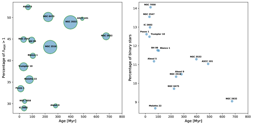
Figure 6: Same as Fig. 3 and 5 but with ages taken from Cantat-Gaudin et al. (2020). Left panel: Percentage of the most massive stars with mass segregation vs age. Right panel: Percentage of binary stars vs age.