Specific heat of Gd³⁺- and Eu²⁺-based magnetic compounds

Abstract

We have studied theoretically the specific heat of a large number of non-frustrated magnetic structures described by the Heisenberg model for systems with total angular momentum $J=7/2$, which corresponds to the 4f⁷ configuration of Gd⁺³ and Eu⁺². For a given critical temperature (controlled by the magnitude of the exchange interactions) we find that to a large accuracy, the specific heat is controlled by two parameters: the effective number of neighbors (which controls the importance of quantum fluctuations) and the axial anisotropy. Using these two parameters we fit the specific heat of four Gd compounds and two Eu compounds obtaining a remarkable agreement. Another Gd compound has been fitted previously. Our work opens the possibility of describing the specific heat of non-frustrated 4f⁷ systems within a general framework.

I Introduction

Rare-earth-based materials are of great interest in both basic and applied condensed matter physics, showing a plethora of captivating fundamental physical phenomena, like unconventional superconductivity Mathur et al. (1998); Shioda et al. (2021), Kondo effect Kobayashi et al. (2008); Romero et al. (2013); Magnavita et al. (2016), quantum criticality Alvarez et al. (2004), quadrupolar order and frustration Watanuki et al. (2005); Okuyama et al. (2005); Ji et al. (2007); Song et al. (2020); Franco et al. (2024).

The specific heat of magnetic materials containing rare earths is typically highly responsive to the environment surrounding the rare earth ions. This sensitivity arises from the splitting of the 4f orbitals by the crystal field and the consequent splitting of the total angular momentum $J$ due to strong spin-orbit coupling. Consequently, excitation energies are influenced by the surrounding environment, thereby affecting the temperature dependence of specific heat.

However, an exception is expected for compounds containing Gd⁺³ and Eu⁺², both of which correspond to the 4f⁷ configuration. In this case, the ground-state multiplet constructed by Hund rules is ${}^{8}S_{7/2}$, which correspond to total spin $S=7/2$, total orbital angular momentum $L=0$ and total angular momentum $J=7/2$. Since neither the spin nor terms with $L=0$ are affected by crystal field, one expects that the only source of splitting of the ground-state octuplet is the exchange interaction between rare-earth ions responsible for the magnetic structure of the compound. This is true as a first approximation. In fact we will show that the specific heat of five Gd compounds can be well fitted ignoring crystal-field effects.

Nevertheless, as a consequence of the spin-orbit coupling, the ground-state multiplet acquires some admixture of ${}^{6}P_{7/2}$ with $L=1$. The explicit calculation has been done in Appendix B of Ref. Betancourth et al., 2019, where it has been estimated that the amount of the excited multiplet in the ground state is $\sim 3\%$. Terms with $L=1$ are not affected by cubic crystal fields but are sensitive to lower symmetries. In particular, they are affected by an axial term, which (using Wigner-Eckart theorem) can be written in the form $H_{K}=K[3J^{2}_{z}-J(J+1)]$, where $K$ is expected to be small.

Even if $H_{K}$ can be neglected, systematic deviations of the observed magnetic contribution to the specific heat $C(T)$ in Gd-based compounds from the corresponding mean field result were observed since long time ago, pointing to the importance of quantum fluctuations. The early measurements of $C(T)$ on GdNi₅ Szewczyk et al. (1992) were compared with calculations in the molecular field approximation for $T<T_{C}=32$ K, where $T_{C}$ is the critical temperature, with good agreement. However the authors recognize evident discrepancies at low temperature and in the vicinity of $T_{C}$ that can be attributed to “short-range ordering effects not taken into account”. Simultaneous measurements of $C(T)$ on other Gd compounds Bouvier et al. (1991) show more significant deviations from the mean-field result. The origin of such deviations was investigated introducing modulations in the amplitude of the magnetic moments in the mean-field approximation Blanco et al. (1991). Such a model describes different possibilities of the observed temperature dependence of $C(T)$ for $T<T_{C}$. However, some compounds clearly escape from those predictions specially concerning observed magnetic fluctuations right above $T_{C}$.

Recent research on Eu²⁺ based compounds show similar shortcomings of the mean-field approach Kumar et al. (2010); Giovannini et al. (2021). The fact that Eu²⁺ has a much larger atomic volume and therefore may participate in the formation of very different crystalline structures indicates that the observed deviations is an intrinsic characteristic of the magnetic interactions and not dependent from crystalline symmetries nor the sign of the interactions. Therefore, for a quantitative explanation of the observed $C(T)$, it is necessary to include quantum fluctuations and go beyond mean field.

In this work we report the specific heat of a large number of structures described by a Heisenberg Hamiltonian containing exchange interactions at different distances

$$H_{0}=\sum_{i,\delta}J_{\delta}\mathbf{S}_{i}\cdot\mathbf{S}_{i+\delta}/2,$$ (1)

where $\mathbf{S}_{i}$ denotes the spin 7/2 at site $i$, $\delta$ labels the non-equivalent space vectors connecting different spins at short distances (nearest and possibly further neighbors) and $J_{\delta}$ is the corresponding exchange interaction.

The theoretically studied magnetic structures are non frustrated. They correspond to either ferromagnetic interactions or non-frustrated antiferromagnetic ones. We find that the specific heat of all these structures can be characterized to a large degree of accuracy by two parameters: i) the effective number of neighbors (to be defined more precisely below) and ii) the magnetic anisotropy defined by $H_{K}$ at each site. Using these two parameters we fit the reported specific heat as a function of temperature for six compounds obtaining an impressive agreement.

The effect of fluctuations on the specific heat of a spin system described by the Heisenberg model is expected to decrease as the number of neighboring spins increases. We can draw an analogy to a binary random distribution (which would correspond to spin 1/2). It is known that after $N$ attempts in a binary random distribution $x$ with probabilities $p$ and $1-p$ for the values $x=1$ and $x=-1$ respectively, the mean value (proportional to the magnetic moment) is $\langle x\rangle=(2p-1)N$ and the standard deviation is $\sqrt{\langle x^{2}\rangle-\langle x\rangle^{2}}=2\sqrt{Np(1-p)}$. Therefore, the ratio between the standard deviation and the mean value decreases as $1/\sqrt{N}$. Similarly in our quantum Heisenberg model, one expects that as the number of neighbors increases, the specific heat is more similar to the mean-field result, in which quantum fluctuations are neglected and the effective magnetic field that each ion feels is replaced by its mean value.

Generalizing the above results to the case of a distribution with intensities $\pm|J_{\delta}|$ for $z_{\delta}$ neighbors we obtain after some algebra (see Appendix)

$$\frac{\langle x^{2}\rangle-\langle x\rangle^{2}}{\langle x\rangle^{2}}=\frac{4p(1-p)}{2p-1}r\text{, where~{}~{}}r=\frac{\Sigma_{\delta}z_{\delta}J_{\delta}^{2}}{(\Sigma_{\delta}z_{\delta}|J_{\delta}|)^{2}}=\frac{1}{z}.$$ (2)

Here, $z_{\delta}$ represents the number of neighbors of type $\delta$ (with exchange interaction $J_{\delta}$), and the summation goes over all types of neighbors. The quantity $z=1/r$ defined by Eq. (2) captures the effective number of neighbors, taking into account the strength ($J_{\delta}^{2}$) and number ($z_{\delta}$) of each type of interaction. Remarkably, for unfrustrated systems, the observed specific heat depends mainly on this effective number of neighbors $z$, independent of the specific lattice structure. For larger $z$ (higher coordination number), the results approach the mean-field ones, where quantum fluctuations are suppressed. Conversely, for lower $z$ (fewer neighbors), quantum fluctuations become more important, leading to a smaller specific heat below the critical temperature $T_{C}$ and a larger specific heat above $T_{C}$. Explicit calculations are shown in Section III.

Moreover, for some actual systems, the effect of the axial anisotropy $H_{K}$ becomes important, redistributing the entropy below $T_{C}$ (see Section IV).

Using the above two parameters for simple lattices, and the known value of $T_{C}$, we have fitted the data for the specific heat of GdNi₃Ga₉, GdCoIn₅, GdCu₂Ge₂, GdNiSi₃, Eu₂Pd₃Sn₃, and EuPdSn₂. The corresponding results are presented in Section VI. Using essentially the same method, the specific heat of GdCoIn₅ has been fitted in Ref. Facio et al., 2015.

II Methods

We have calculated the specific heat of a large number of magnetic structures form the numerical derivative of the internal energy as a function of temperature. This energy was obtained using quantum Monte Carlo (QMC) simulations from the ALPS libraries (“dirloop_sse” package) Albuquerque et al. (2007); Bauer et al. (2011). Our calculations encompassed a wide range of system sizes, reaching up to $8\times 30^{3}$ magnetic moments.

To generate the lattice configurations for the ALPS simulations, we utilized the “SUNNY” package Dahlbom et al. (2024) in conjunction with crystallographic information files (CIF) obtained from public repositories. Specifically, CIF files for Fe in simple cubic (SC), body-centered cubic (BCC), hexagonal close-packed (HCP), and face-centered cubic (FCC) structures, as well as C in diamond, MgAl₂Cu (for EuPdSn₂), and ErNi₃Al₉, were retrieved from the Materials Project Jain et al. (2013) database. The ErNi₃Al₉ CIF file was obtained from the Crystallography Open Database Gražulis et al. (2009) using data from reference Gladyshevskii et al., 1993. In each case, the magnetic structure was created by replacing C, Fe, Mg, or Er with a spin moment $S=7/2$.

For all lattices, we adopted a rectangular cuboid supercell geometry as the conventional unit cell. This choice resulted in a varying number of sites within the supercell, with the diamond lattice requiring the largest (8 sites). The simulations were performed on systems containing $N^{3}$ supercells with periodic boundary conditions, typically with $N=10$, $20$, and $30$. For cases exhibiting size effects, the results were extrapolated to the thermodynamic limit assuming a $1/N$ dependence.

The well-known sign problem Pan and Meng (2024) associated with QMC simulations limited our investigation to non-frustrated magnetic structures. At low temperatures, the number of Monte Carlo steps required for statistically reliable results increases exponentially. Consequently, the internal energy was primarily computed in a temperature range between $0.2T_{C}$ and $2T_{C}$, where $T_{C}$ is the critical temperature of the system. In a few cases, the simulations were extended to $0.1T_{C}$ at low temperatures. However, the reliability of the results below $0.2T_{C}$ is limited.

The coordination number (number of neighbors included) for each lattice is provided in parentheses after its name. For example, FCC(18) refers to a face-centered cubic lattice with 12 first neighbors and 6 second-nearest neighbors. Only for the simple cubic case, SC(14), we consider a scenario including both the 8 nearest neighbors (NN) and the 6 third NN. In other cases, additional neighbor shells were included by increasing the considered neighbor radius $d$.

Our theoretical results for the specific heat for all lattices used here are available in Garcia, D. J., Sereni, J., Aligia, A. A., .

III Role of the effective number of neighbors

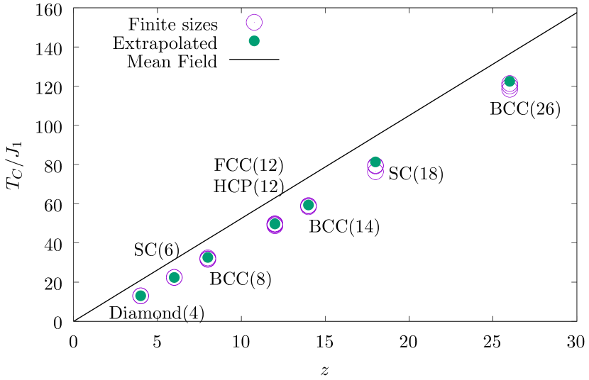
Figure 1: Critical temperature as a function of the number of neighbors for several ferromagnetic structures, sizes ($N=10,20,30$) and extrapolated value. The straight line denotes the mean-field value $T_{C}^{\text{ MF}}$.

In this Section we report our results for the specific heat and critical temperature for several simple lattices as a function of the number of neighbors that interact with a given site. For simplicity in all lattices considered, all sites are equivalent, and we assume all $J_{\delta}=J_{1}$, where $J_{1}$ is the NN interaction, up to a certain distance $d$ and 0 for longer distances. Therefore the effective number of neighbors $z=\Sigma_{\delta}z_{\delta}$ is just the sum of all neighbors within a sphere of radius $d$. In Section V we discuss more general cases showing that the results are not severely affected by this assumption.

Most of our studies assume ferromagnetic interactions ($J_{1}<0$). In general, the results for the corresponding non-frustrated antiferromagnetic structures are very similar, particularly for $z>6$, except at very low temperatures, for which the specific heat dominated by magnons behaves as $T^{3/2}$ ($T^{3}$) for ferro- (antiferro-) magnetic structures.

In Fig. 1 we show the critical temperature $T_{C}$ as a function of $z$ for the different structures considered. The calculations have been done in finite systems containing $N^{3}$ conventional unit cells, with $N=10$, 20 and 30, as explained in Section II. The extrapolated value is also indicated in the figure.

As expected, $T_{C}$ increases almost linearly with $z$ as the mean-field value $T_{C}^{\text{ MF}}$ (the effective magnetic field due to the interactions is proportional to $zJ_{1}$, see Section IV.1), but it is lower than $T_{C}^{\text{ MF}}$, particularly for low $z$ due to the effect of the quantum fluctuations, which is larger for low $z$. For large enough $z$ one expects that $T_{C}$ and $T_{C}^{\text{ MF}}$ coincide. However, for large $z$ in a finite system with periodic boundary conditions, the effective coordination is smaller when the range of the interactions $d$ becomes of the order of the system size, because neighbors at different distances coincide, and it is not possible to reach this limit with our method.

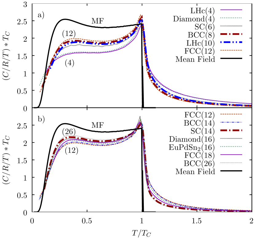
Figure 2: (Color online) Specific heat over temperature as a function of temperature for several ferromagnetic structures with different effective number of neighbors $z$. Top:$z\leq 12$. Bottom: $z\geq 12$. There is an almost perfect superposition between HCP and FCC for $z=12$, among SC, FCC and HCP for $z=18$, and among SC, BCC and the EuPdSn₂ structure for $z=26$. Therefore only one of the curves for each of these three sets is shown. LHc(4) corresponds to the layered honeycomb structure with $z=4$.

In Fig. 2 we show the results for the specific heat as a function of temperature for a large number of ferromagnetic structures with different number of magnetic neighbors $z$. Also shown is the mean-field result which corresponds to the limit $z\rightarrow\infty$. This result shows the larger $C$ for $T<T_{C}$, while $C=0$ for $T>T_{C}$. In contrast, $C$ for a honeycomb layered system with $z=4$ (three NN within the plane of the honeycomb layer and one above or below the layer in alternating sites) shows the smaller specific heat below $T_{C}$ and the largest one above $T_{C}$. Note that the diamond structure, which is completely different from the previous one, but also has $z=4$, has a very similar specific heat.

Increasing $z$ from 4 to 6, the specific heat of the simple cubic structure with six NN displays the expected trend of increasing (decreasing) $C$ below (above) $T_{C}$. Increasing $z$ up to 14 using the bcc structure with 8 NN and 6 next NN (NNN), the same trend is in general observed. However, the specific heat of the honeycomb lattice (with the four links as described before and adding 6 second neighbors in the plane) with $z=10$ lies slightly below the cubic bcc with $z=8$ NN for $T\sim 0.5T_{C}$. In addition, somewhat unexpected is the result for the simple cubic structure including 8 NN and 6 third NN, whose $C$ at $T\sim 0.5T_{C}$ is greater than the corresponding one of the above mentioned BCC structure with the same $z=14$, and also greater than the specific heat of one structure with $z=16$ and two structures with $z=18$. Nevertheless, except for this case and the above mentioned inversion between $z=8$ and 10, the specific heat is very similar for different structures with the same $z$ and increases with increasing $z$ at intermediate temperature $T\sim 0.5T_{C}$.

IV Effect of anisotropy

In this Section we address the role of the anisotropy first in mean field, and later we incorporate the effect of quantum fluctuations.

IV.1 Mean-field approximation

In this subsection, we discuss the effect of the term $H_{K}=K[3J^{2}_{z}-J(J+1)]$ on the specific heat calculated in the mean-field approximation, in which it is assumed that each site is subjected to a constant effective magnetic field that results from the interaction with the remaining sites. We assume that all sites are equivalent and there is no external magnetic field. For simplicity we restrict the analysis to the easy axis case $K<0$ for which the spins point in the direction of the anisotropy. In the next subsection, both signs of $K$ and the effects of quantum fluctuations will be considered.

The effective magnetic field $B_{\text{eff}}$ is given by

$$\tilde{B}=g\mu_{B}B_{\text{eff}}=I\langle J_{z}\rangle\text{,~{}~{}~{} }\langle J_{z}\rangle=\sum\limits_{M=-J}^{J}\frac{Me^{-\beta E_{M}}}{Z}\text{,~{}~{}~{} }Z=\sum\limits_{M=-J}^{J}e^{-\beta E_{M}},$$ (3)

where $g$ is the gyromagnetic factor, $\mu_{B}$ is the Bohr magneton, $I=\Sigma_{\delta}z_{\delta}J_{\delta}$ is the sum of all interactions ($z_{\delta}$ is the number of neighbors at distance $\delta$ and $J_{\delta}$ its intensity), $\beta=1/(k_{B}T)$ where $T$ is the temperature and $k_{B}$ is the Boltzmann constant. The energies $E_{M}$ for each eigenvalue $M$ of the operator $J_{z}$ is given by

$$E_{M}=-\tilde{B}M+K[3M^{2}-J(J+1)].$$ (4)

Eqs. (3) and (4) permit to determine $\tilde{B}$ selfconsistently. In the limit $\tilde{B}\rightarrow 0$ one obtains an equation for the critical temperature

$$k_{B}T_{C}^{\text{ MF}}=I\langle J^{2}_{z}\rangle\text{, with~{}~{}}\langle J^{2}_{z}\rangle=\sum\limits_{M=-J}^{J}\frac{M^{2}e^{-\beta E_{M}}}{Z}.$$ (5)

The specific heat is obtained from the numerical derivative of the entropy $S$ with respect to the temperature

$$C=T\frac{dS}{dT}\text{,~{}~{}~{} }S=\sum\limits_{M=-J}^{J}p_{M}\ln p_{M}\text{,~{}~{}~{} }p_{M}=\frac{e^{-\beta E_{M}}}{Z}$$ (6)

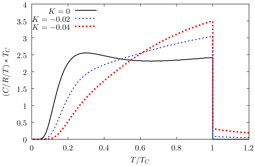
Figure 3: (Color online) Specific heat over temperature as a function of temperature for several anisotropies in the mean-field approximation.

In Fig. 3 we show the resulting effect of the axial anisotropy on the specific heat keeping the value of $k_{B}T_{C}=1$ constant, as the unit of energy. For $K=0$, the value of the intensity for a given $T_{C}$ is $I=3k_{B}T_{C}/[J(J+1)]$, leading to $I=4/21\sim 0.190$ for $k_{B}T_{C}=1$.

For $K=-0.02$, we obtain $I=0.1531$ from Eq. (5). This is because the expectation value $\langle J^{2}_{z}\rangle$ that enters Eq. (5) is larger for $K<0$ and should be compensated with a smaller $I$. In addition, since the values of high $J_{z}$ projection $|M|$ are favored, the effective magnetic field is more efficient than for $K=0$ in splitting the lowest energy levels and therefore the entropy and the specific heat decrease for $T<0.4T_{C}$ with respect to the isotropic case. This is compensated by an increase in $C/T$ for $0.5T_{C}<T<T_{C}$.

For $K=-0.04$, $I$ decreases further to $I=0.1263$, and the changes in the specific heat are more marked in the same direction. For large negative $K$, $I=1/(7/2)^{2}\sim 0.0816$.

IV.2 Beyond mean field

In this Section we discuss the effect of anisotropy in cases where the fluctuations of the effective field are also included.

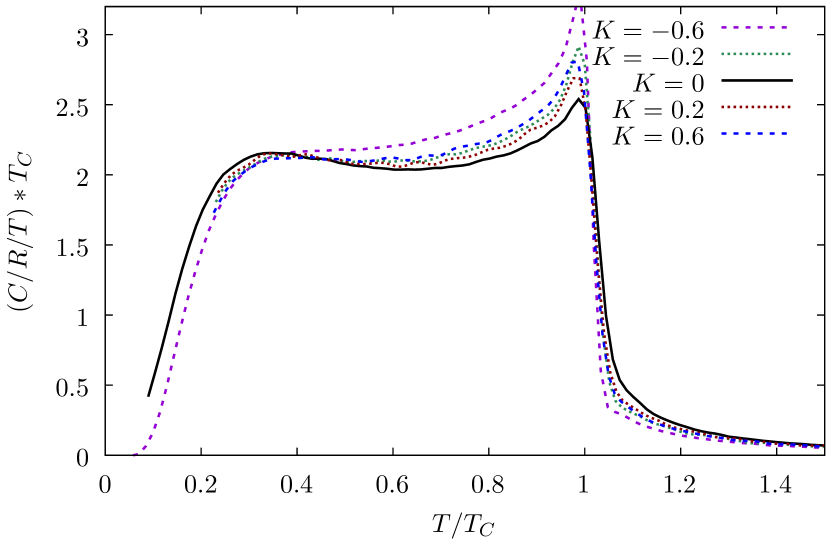
Figure 4: (Color online) Specific heat over temperature as a function of temperature for several anisotropies for the simple cubic structure including 8 NN and 6 fourth NN with $J_{\delta}=-1$.

In Fig. 4 we show how the specific heat for a structure with $z=14$ is modified by the addition of $H_{K}$. The results are qualitatively the same as in the mean-field case for $T<T_{C}$. Addition of the anisotropy term shifts the entropy from the region $T<0.5T_{C}$ mainly to the region $0.5T_{C}<T<T_{C}$, and the effect is more pronounced for negative $K$.

However, in contrast to the mean-field case, addition of the anisotropy term decreases the specific heat for $T>T_{C}$. This reduction is expected because the specific heat in this region primarily results from quantum fluctuations, which are diminished by the energy level splitting induced by $H_{K}$.

V Comparison of different structures with the same effective number of neighbors

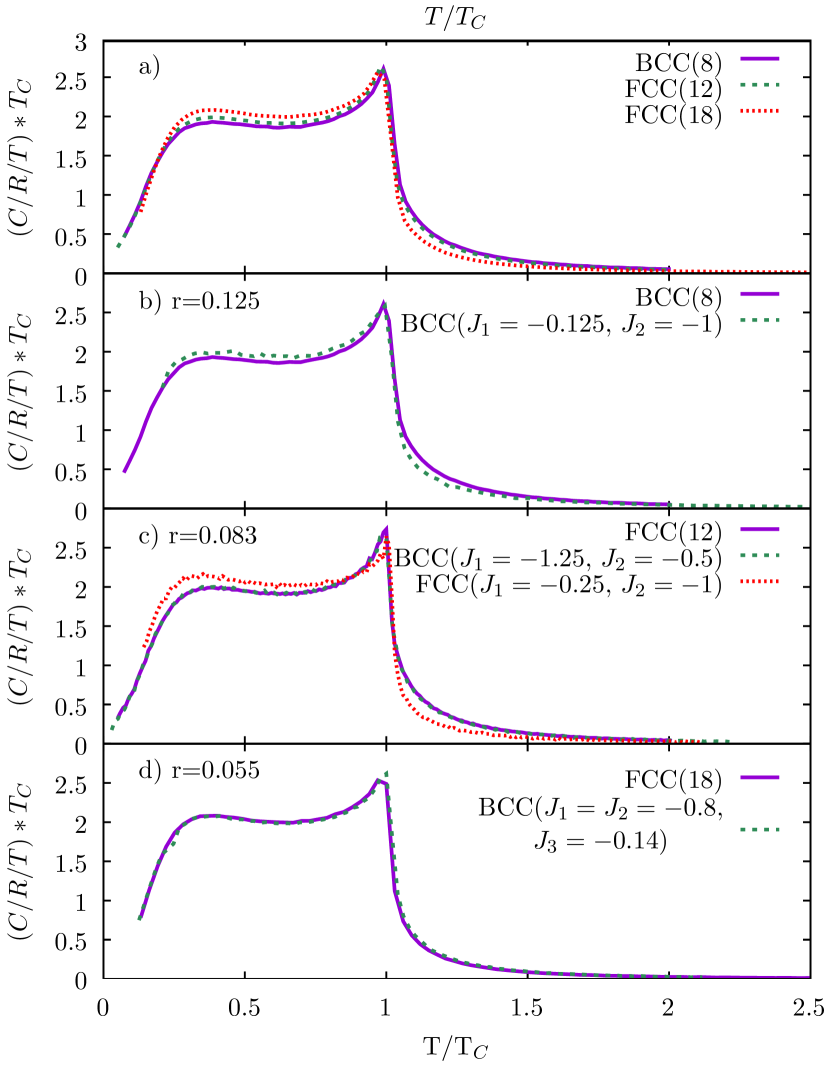
Figure 5: (Color online) Specific heat over temperature as a function of temperature for several structures with different values of $r$ defined by Eq. (2). Top left: several structures with $J_{\delta}=-1$ and different $r$. The rest of the panels show the effect of changing $J_{\delta}$ keeping the same $r$.

In Section III we have discussed the effect of increasing number of neighbors $z$ in the specific heat keeping for simplicity $J_{\delta}=J_{1}$. Here we investigate the effect of changing $J_{\delta}$ for first, second and possibly third NN, keeping the same $r$ [see Eq. (2)], which corresponds to the inverse of the effective number of neighbors $z$. In Fig. 5 (b) we show the comparison for a moderately small $z$: a cubic bcc structure with 8 NN and 6 fourth NN. We compare that case of NN interaction $J_{1}=-1$ and NNN interaction $J_{2}=0$ with $J_{1}=-1/8$ and $J_{2}=-1$. In spite of the radical change in the magnitude of the interactions, the specific heats are rather similar.

In Fig. 5 (c) we show a similar comparison for an fcc structure with different combinations of $J_{1}$ and $J_{2}$. Again the results are similar, except for the case in which the dominant interaction is changed drastically from NN to NNN. When the dominant interaction is that of NNN, the specific heat is larger and the difference is of the order of that between different $z$ for $J_{1}=-1$ (Fig. 5 (a)). Finally in (Fig. 5 (d)) we show a similar comparison for a larger $z$. In this case, the agreement between the two curves is excellent.

In conclusion, except for extreme cases, the magnitude of the specific heat at $T\sim T_{C}/2$ is mainly determined by the effective number of neighbors $z=1/r$. This result is significant, because it allows us to predict the expected specific heat taking into account the effective number of neighbors with a relative independence of the detailed magnetic structure.

VI Fits of experimental data

In this Section, we present fits of the specific heat of six compounds: GdNi₃Ga₉, GdCu₂Ge₂, GdNiSi₃, Eu₂Pd₃Sn₃, and EuPdSn₂. Previously, the specific heat of GdCoIn₅ has been fitted Facio et al. (2015).

The fitting parameters are the known $T_{C}$, which determines the magnitude of the interactions $J_{\delta}$ assumed equal, the number of neighbors $z$ and for the Eu compounds, the anisotropy $K$. The Gd compounds could be fitted with $K=0$. The results are presented in Fig. 6. The Gd and Eu compounds are ordered with increasing effective number of neighbors $z$ in the fit.

GdNi₃Ga₉ Silva (2017); Nakamura et al. (2023) clearly correspond to a low coordination number ($z=4$). The honeycomb lattice described in Section III with antiferromagnetic interactions is similar to the real structure of the material and provides a very good fit. For the rest of the structures, ferromagnetic interactions are assumed.

GdPdBi Jesus et al. (2014) is a half-Heusler structure with antiferromagnetic coupling. We obtain a very good fit assuming also a layered honeycomb lattice as for the previous compound, but with larger number of effective neighbors (10).

GdCu₂Ge₂ Duong (2002) has a BCC structure. Using only the 8 NN interactions, the resulting specific heat is very near the experimental one, although slightly below (above) the experimental one for $T<T_{C}$ ($T>T_{C}$) suggesting that $z$ might be a little bit larger.

For GdNiSi₃ Arantes et al. (2018) a simple cubic structure with $z=26$ including neighbors up to the 3rd coordination shell provides a very good fit of the data. This completes the Gd compounds that we have considered.

In previous work Facio et al. (2015), the specific heat of GdCoIn₅ has been fitted. The compound has a tetragonal structure (near to the simple cubic one). The authors have extrapolated to the thermodynamic limit, the specific heat that corresponds to $z=6$ NN antiferromagnetic interactions, providing an excellent fit of the data.

Now turning to Eu compounds, the specific heat of Eu₂Pd₃Sn I. Čurlík , is very well fitted using a simple cubic structure with 6 NN and 8 fourth NN ($z=14$) with $J_{1}=J_{2}$ and $K=-0.4J_{1}$. Small deviations exist at very low temperatures, where our numerical method is not fully reliable.

Finally, the same simple cubic structure, but with $K=-0.6J_{1}$ provides a very good fit of the specific heat of EuPdSn₂ Čurlík et al. (2018). For temperatures very near $T_{C}$, the theoretical data are a little above (below) the experimental ones for $T<T_{C}$ ($T>T_{C}$)

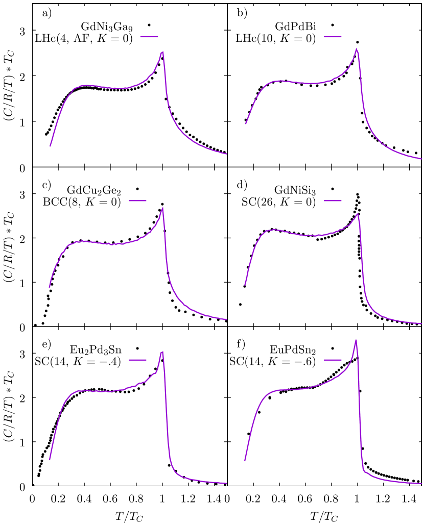
Figure 6: (Color online) Specific heat over temperature as a function of temperature for several compounds and our fit. $K=0$ for the Gd compounds. Experimental data were taken from Refs. Silva, 2017; Nakamura et al., 2023; Jesus et al., 2014; Duong, 2002; Arantes et al., 2018; Čurlík et al., 2018; I. Čurlík, .

VII Summary

Using quantum Monte Carlo, we have calculated the specific heat of a large number of non-frustrated magnetic structures. As expected from mean-field theory, the critical temperature $T_{C}$ increases approximately proportionally to $I=\Sigma_{\delta}z_{\delta}J_{\delta}$, where $J_{\delta}$ is exchange interaction at distance $\delta$, and $z_{\delta}$ is the number of neighbors at this distance. However $T_{C}$ lies below the mean-field value.

Rather surprisingly, we find that the specific heat depends mainly on the effective number of neighbors $z$ [see Eq. (2)] and is not quite sensitive to the particular structure. This allows us to derive general conclusions on the effect of $z$, independently of the particular structure. For large $z$ quantum fluctuations are reduced and the specific heat approaches the mean-field value. Reducing $z$ the specific heat decreases below $T_{C}$ and increases above $T_{C}$ displaying larger tails.

For a quantitative comparison with experiments, it is necessary to consider also an axial anisotropy $H_{K}$ (see Section IV). The origin of $H_{K}$ is due to a small admixture of ${}^{6}P_{7/2}$ in the ground-state multiplet. The presence of a small component with $L=1$ renders the system sensitive to axial crystal fields.

Using $z$ as the only free parameter in addition to the critical temperature, we have fitted the specific heat of four Gd compounds (GdNi₃Ga₉, GdPdBi, GdCu₂Ge₂, and GdNiSi₃). The specific heat of GdCoIn₅ has been fitted previously using the same approach Facio et al. (2015). Curiously, we find that $H_{K}$ can be neglected for these Gd compounds. Including also $K$ as a parameter, we have done the same fitting for two Eu compounds (Eu₂Pd₃Sn₃ and EuPdSn₂). The agreement shown in Fig. 6 is noticeable. It is possible that the larger atomic volume of Eu⁺² renders this ion more susceptible to crystal-field effects.

Note that while most of our calculations have been done on non-frustrated systems, some of the fitted compounds here (GdPdBi and GdNiSi₃), and GdCoIn₅ fitted previously Facio et al. (2015), are expected to have some degree of frustration.

Our work opens the possibility to classify and analyze the specific heat of non-frustrated Gd⁺³ and Eu⁺², at least in a first semiquantitative manner using the above discussed two parameters.

VIII Appendix

Here we calculate the mean value and fluctuations of a random variable $x$ with different intensities. For simplicity we consider only two intensities $J_{1}$ and $J_{2}$. Extension to the general case is straightforward. We consider $z_{1}$ attempts in which the probability of the result $J_{1}$ is $p$ and that of $-J_{1}$ is $q=1-p$. In addition, there are $z_{2}$ attempts with probability $r$ of finding the result $J_{2}$ and $s=1-r$ for the result $-J_{2}$. At the end we will take $r=p$. For non-frustrated systems, both $J_{\delta}$ can be chosen positive. Clearly, the expectation value of $x$ is

$$\langle x\rangle=z_{1}J_{1}(p-q)+z_{2}J_{2}(r-s).$$ (7)

On the other hand, considering the probability of each individual event one has

$$\langle x^{2}\rangle=\sum\limits_{n=0}^{z_{1}}\sum\limits_{m=0}^{z_{2}}\binom{z_{1}}{n}\binom{z_{2}}{m}p^{n}q^{z_{1}-n}r^{m}s^{z_{2}-m}\left[nJ_{1}-(z_{1}-n)J_{1}+mJ_{2}-(z_{2}-m)J_{2}\right]^{2}.$$ (8)

Using the operator

$$O=\left[J_{1}\left(p\frac{\partial}{\partial p}-q\frac{\partial}{\partial q}\right)+J_{2}\left(r\frac{\partial}{\partial r}-s\frac{\partial}{\partial s}\right)\right],\text{ and }(p+q)^{z_{1}}=\sum\limits_{n=0}^{z_{1}}\binom{z_{1}}{n}p^{n}q^{z_{1}-n},$$ (9)

and a similar expression for $(r+s)^{z_{2}}$, in which $p$ and $q$ as well as $r$ and $s$ are taken as independent variables in the derivatives, one realizes that the expectation value Eq. (8) can be written as

$$\langle x^{2}\rangle=O^{2}(p+q)^{z_{1}}(r+s)^{z_{2}}.$$ (10)

Performing the calculation we find after some algebra

$$\langle x^{2}\rangle = J_{1}^{2}z_{1}\left[1+(z_{1}-1)(p-q)^{2}\right]+J_{2}^{2}z_{2}\left[1+(z_{2}-1)(r-s)^{2}\right]$$ (11)

$$+2J_{1}J_{2}z_{1}z_{2}(p-q)(r-s)$$

Using Eqs. (7) and (11), setting $r=p$ and replacing $q=s=1-p$, one finally obtains

$$\frac{\langle x^{2}\rangle-\langle x\rangle^{2}}{\langle x\rangle^{2}}=\frac{4p(1-p)}{2p-1}\frac{z_{1}J_{1}^{2}+z_{2}J_{2}^{2}}{\left(z_{1}J_{1}+z_{2}J_{2}\right)^{2}}$$ (12)

References

- Mathur et al. (1998) N. D. Mathur, F. M. Grosche, S. R. Julian, I. R. Walker, D. M. Freye, R. K. W. Haselwimmer, and G. G. Lonzarich, Nature 394, 39 (1998), ISSN 1476-4687, URL https://doi.org/10.1038/27838.
- Shioda et al. (2021) N. Shioda, K. Kumeda, H. Fukazawa, T. Ohama, Y. Kohori, D. Das, J. Bławat, D. Kaczorowski, and K. Sugimoto, Phys. Rev. B 104, 245119 (2021), URL https://link.aps.org/doi/10.1103/PhysRevB.104.245119.
- Kobayashi et al. (2008) Y. Kobayashi, T. Onimaru, M. A. Avila, K. Sasai, M. Soda, K. Hirota, and T. Takabatake, Journal of the Physical Society of Japan 77, 124701 (2008), eprint https://doi.org/10.1143/JPSJ.77.124701, URL https://doi.org/10.1143/JPSJ.77.124701.
- Romero et al. (2013) M. A. Romero, A. A. Aligia, J. G. Sereni, and G. Nieva, Journal of Physics: Condensed Matter 26, 025602 (2013), URL https://dx.doi.org/10.1088/0953-8984/26/2/025602.
- Magnavita et al. (2016) E. Magnavita, C. Rettori, J. Osorio-Guillén, F. Ferreira, L. Mendonça-Ferreira, M. Avila, and R. Ribeiro, Journal of Alloys and Compounds 669, 60 (2016), ISSN 0925-8388, URL https://www.sciencedirect.com/science/article/pii/S0925838816302079.
- Alvarez et al. (2004) J. V. Alvarez, H. Rieger, and A. Zheludev, Phys. Rev. Lett. 93, 156401 (2004), URL https://link.aps.org/doi/10.1103/PhysRevLett.93.156401.
- Watanuki et al. (2005) R. Watanuki, G. Sato, K. Suzuki, M. Ishihara, T. Yanagisawa, Y. Nemoto, and T. Goto, Journal of the Physical Society of Japan 74, 2169 (2005), eprint https://doi.org/10.1143/JPSJ.74.2169, URL https://doi.org/10.1143/JPSJ.74.2169.
- Okuyama et al. (2005) D. Okuyama, T. Matsumura, H. Nakao, and Y. Murakami, Journal of the Physical Society of Japan 74, 2434 (2005), eprint https://doi.org/10.1143/JPSJ.74.2434, URL https://doi.org/10.1143/JPSJ.74.2434.
- Ji et al. (2007) S. Ji, C. Song, J. Koo, J. Park, Y. J. Park, K.-B. Lee, S. Lee, J.-G. Park, J. Y. Kim, B. K. Cho, et al., Phys. Rev. Lett. 99, 076401 (2007), URL https://link.aps.org/doi/10.1103/PhysRevLett.99.076401.
- Song et al. (2020) M. S. Song, K. K. Cho, B. Y. Kang, S. B. Lee, and B. K. Cho, Scientific Reports 10, 803 (2020), ISSN 2045-2322, URL https://doi.org/10.1038/s41598-020-57621-7.
- Franco et al. (2024) D. G. Franco, R. Avalos, D. Hafner, K. A. Modic, Y. Prots, O. Stockert, A. Hoser, P. J. W. Moll, M. Brando, A. A. Aligia, et al., Phys. Rev. B 109, 054405 (2024), URL https://link.aps.org/doi/10.1103/PhysRevB.109.054405.
- Betancourth et al. (2019) D. Betancourth, V. F. Correa, J. I. Facio, J. Fernández, V. Vildosola, R. Lora-Serrano, J. M. Cadogan, A. A. Aligia, P. S. Cornaglia, and D. J. García, Physical Review B 99, 134406 (2019).
- Szewczyk et al. (1992) A. Szewczyk, R. Radwański, J. Franse, and H. Nakotte, Journal of Magnetism and Magnetic Materials 104-107, 1319 (1992), ISSN 0304-8853, proceedings of the International Conference on Magnetism, Part II, URL https://www.sciencedirect.com/science/article/pii/030488539290600S.
- Bouvier et al. (1991) M. Bouvier, P. Lethuillier, and D. Schmitt, Phys. Rev. B 43, 13137 (1991), URL https://link.aps.org/doi/10.1103/PhysRevB.43.13137.
- Blanco et al. (1991) J. A. Blanco, D. Gignoux, and D. Schmitt, Phys. Rev. B 43, 13145 (1991), URL https://link.aps.org/doi/10.1103/PhysRevB.43.13145.
- Kumar et al. (2010) N. Kumar, S. K. Dhar, A. Thamizhavel, P. Bonville, and P. Manfrinetti, Phys. Rev. B 81, 144414 (2010), URL https://link.aps.org/doi/10.1103/PhysRevB.81.144414.
- Giovannini et al. (2021) M. Giovannini, I. Čurlík, R. Freccero, P. Solokha, M. Reiffers, and J. Sereni, Inorg Chem 60, 8085 (2021).
- Facio et al. (2015) J. I. Facio, D. Betancourth, P. Pedrazzini, V. F. Correa, V. Vildosola, D. J. García, and P. S. Cornaglia, Phys. Rev. B 91, 014409 (2015), URL https://link.aps.org/doi/10.1103/PhysRevB.91.014409.
- Albuquerque et al. (2007) A. Albuquerque, F. Alet, P. Corboz, P. Dayal, A. Feiguin, S. Fuchs, L. Gamper, E. Gull, S. Gürtler, A. Honecker, et al., Journal of Magnetism and Magnetic Materials 310, 1187 (2007), ISSN 0304-8853, proceedings of the 17th International Conference on Magnetism, URL https://www.sciencedirect.com/science/article/pii/S0304885306014983.
- Bauer et al. (2011) B. Bauer, L. D. Carr, H. G. Evertz, A. Feiguin, J. Freire, S. Fuchs, L. Gamper, J. Gukelberger, E. Gull, S. Guertler, et al., Journal of Statistical Mechanics: Theory and Experiment 2011, P05001 (2011), URL https://dx.doi.org/10.1088/1742-5468/2011/05/P05001.
- Dahlbom et al. (2024) D. Dahlbom, F. T. Brooks, M. S. Wilson, S. Chi, A. I. Kolesnikov, M. B. Stone, H. Cao, Y.-W. Li, K. Barros, M. Mourigal, C. D. Batista, X. Bai, Physical Review B 109, 014427 (2024).
- Jain et al. (2013) A. Jain, S. P. Ong, G. Hautier, W. Chen, W. D. Richards, S. Dacek, S. Cholia, D. Gunter, D. Skinner, G. Ceder, et al., APL Materials 1, 011002 (2013), ISSN 2166-532X, eprint https://pubs.aip.org/aip/apm/article-pdf/doi/10.1063/1.4812323/13163869/011002_1_online.pdf, URL https://doi.org/10.1063/1.4812323.
- Gražulis et al. (2009) S. Gražulis, D. Chateigner, R. T. Downs, A. F. T. Yokochi, M. Quirós, L. Lutterotti, E. Manakova, J. Butkus, P. Moeck, and A. Le Bail, Journal of Applied Crystallography 42, 726 (2009), URL https://doi.org/10.1107/S0021889809016690.
- Gladyshevskii et al. (1993) R. E. Gladyshevskii, K. Cenzual, H. D. Flack, and E. Parthé, Acta Crystallographica Section B 49, 468 (1993), URL https://doi.org/10.1107/S010876819201173X.
- Pan and Meng (2024) G. Pan and Z. Y. Meng, The sign problem in quantum Monte Carlo simulations (Elsevier, 2024), p. 879–893, ISBN 9780323914086, URL http://dx.doi.org/10.1016/B978-0-323-90800-9.00095-0.
- (26) Garcia, D. J., Sereni, J., Aligia, A. A., Energy and specific heat for magnetic crystals, Zenodo data set, URL https://doi.org/10.5281/zenodo.12659008.
- Silva (2017) L. d. S. Silva, Ph.D. thesis, Universidade Federal de Sergipe (2017).
- Nakamura et al. (2023) S. Nakamura, T. Matsumura, K. Ohashi, H. Suzuki, M. Tsukagoshi, K. Kurauchi, H. Nakao, and S. Ohara, Physical Review B 108, 104422 (2023).
- Jesus et al. (2014) C. Jesus, P. Rosa, T. Garitezi, G. Lesseux, R. Urbano, C. Rettori, and P. Pagliuso, Solid State Communications 177, 95 (2014), ISSN 0038-1098, URL https://www.sciencedirect.com/science/article/pii/S0038109813004602.
- Duong (2002) N. P. Duong, Ph.D. thesis, University of Amsterdam (2002).
- Arantes et al. (2018) F. R. Arantes, D. Aristizábal-Giraldo, S. H. Masunaga, F. N. Costa, F. F. Ferreira, T. Takabatake, L. Mendonca-Ferreira, R. A. Ribeiro, and M. A. Avila, Phys. Rev. Mater. 2, 044402 (2018), URL https://link.aps.org/doi/10.1103/PhysRevMaterials.2.044402.
- (32) S. I. Čurlík, University of Prešov, private communication.
- Čurlík et al. (2018) I. Čurlík, M. Giovannini, F. Gastaldo, A. M. Strydom, M. Reiffers, and J. G. Sereni, Journal of Physics: Condensed Matter 30, 495802 (2018), URL https://dx.doi.org/10.1088/1361-648X/aae7ae.