Tangent Space Causal Inference: Leveraging Vector Fields for Causal Discovery in Dynamical Systems
Abstract
Causal discovery with time series data remains a challenging yet increasingly important task across many scientific domains. Convergent cross mapping (CCM) and related methods have been proposed to study time series that are generated by dynamical systems, where traditional approaches like Granger causality are unreliable. However, CCM often yields inaccurate results depending upon the quality of the data. We propose the Tangent Space Causal Inference (TSCI) method for detecting causalities in dynamical systems. TSCI works by considering vector fields as explicit representations of the systems’ dynamics and checks for the degree of synchronization between the learned vector fields. The TSCI approach is model-agnostic and can be used as a drop-in replacement for CCM and its generalizations. We first present a basic version of the TSCI algorithm, which is shown to be more effective than the basic CCM algorithm with very little additional computation. We additionally present augmented versions of TSCI that leverage the expressive power of latent variable models and deep learning. We validate our theory on standard systems, and we demonstrate improved causal inference performance across a number of benchmark tasks.
1 Introduction
The discovery of causal relationships is one of the most fundamental goals of scientific work. When causal relationships are known and understood, we can explain the behavior of a system and understand how our actions or interventions upon the system will affect its behavior [27]. This kind of reasoning is fundamental in many problem domains, such as medicine, environmental policy, and economics. However, it is not always possible to perform interventions and observe their effects. For example, medical practitioners might only have one chance to prescribe a medication to help a patient. As another example, an ecologist might find that performing a large experiment is forbiddingly expensive or otherwise infeasible. Due to these concerns, there remains a great interest in the problem of observational causal inference, where one infers causation without manipulating the system under study directly.
For time series data, the most prominent tool for observational causal inference is Granger causality [15]. Granger causality operates on the assumption that if one system (the cause) is driving changes in another system (the effect), then the cause should have unique information about what will happen to the effect. This is encoded in an assumption called separability, which posits that the information needed to predict the future behavior of the effect is not contained in the effect itself. However, the separability condition runs counter to the behavior of coupled dynamical systems: if long histories of the effect can forecast the cause, then an autoregressive model with the appropriate lag may forecast the effect from itself. This effect is explored in the supplementary materials of [12, 41], and we give an example in Appendix B. Since systems with (approximately) dynamical behavior are ubiquitous in many application domains, alternative methods have become of interest.
To address the failures of Granger causality in coupled dynamical systems Sugihara et al. [41] proposed the convergent cross mapping (CCM) method, which directly takes advantage of the topological properties of dynamical systems. CCM can be seen as an adaption of earlier work that studied the synchronization of dynamical systems [2, 29, 35] into an algorithmic procedure for detecting causalities between time series. Using Takens’ theorem, a well-known result in dynamical systems theory [42], CCM attempts to detect causality by reconstructing the state space of a given time series, and then learning a time-invariant function that maps between reconstructed state spaces, called a cross map. The key assumption is that the cross map only exists if the original systems were dynamically coupled. In this sense, the “causality” of CCM deviates from the popular Pearlian framework [27], and is better interpreted as identifying which variables “drive” or “force” a dynamical system based on observational data.111Although not typically interpreted as such, cross maps have been suggested to be interpretable in a Pearlian causal framework via the do operator [12]. Building upon this framework, several extensions of CCM have been proposed to address various technicalities and caveats of the approach and to generalize the method to new domains. However, the CCM test statistic is difficult to interpret and does not admit a simple decision rule. CCM also does not explicitly learn a cross map function.
To improve upon CCM, we propose Tangent Space Causal Inference (TSCI). TSCI detects causation between dynamical systems by explicitly checking if the dynamics of one system map on to the other. The proposed method can be seen as a drop-in replacement for the CCM test, providing an interpretable and principled alternative while remaining compatible with many of the extensions of CCM. Furthermore, the proposed method is model agnostic, meaning that it can be adapted to any method used to learn the cross map function, including multilayer perception (MLP) networks, splines, or Gaussian process regression. The only major assumption of TSCI is that the time series under study were generated by continuous time dynamical systems (i.e, by systems of differential equations), which is a standard assumption in a number of physical systems [36]. As a result, TSCI is applicable to many of the same problems as CCM.
1.1 Related Work
Causal representation learning. The primary function of Takens’ theorem in the CCM method is to yield a representation of a system’s latent state so that it may be used for cross mapping. As a result, numerous generalizations of Takens’ theorem emerged in the following decades [32, 33, 40]. Causal representation learning aims to learn hidden variables from high dimensional observations [1], and a principle task is to decipher the causal relationships between many, possibly redundant, observations of a system [30]. In such cases, methods of dimensionality reduction can be applied to extract causal variables from the raw observations [31]. This is particularly important in the processing of large, spatio-temporal data sets [36, 43]. Some authors have proposed that CCM can be improved by aggregating data from multiple sources into the reconstruction of the latent states [7, 45], which requires an awareness of how the observation data relate to the causal variables of interest.
Causal discovery with cross maps. CCM has popularized the use of cross maps as a tool for causal inference, and many variations and improvements of the basic CCM methodology have been proposed. Some of these works aim to improve the reconstruction of latent states in these models by using a Bayesian approach to latent state inference [13], where the approach is adapted for spatial/geographic data [14] or modified for sporadically sampled time series [12]. Additionally, several improvements have suggested changing the way that a cross map is detected: some authors have recommended varying the library length [25] or time delaying the cross mapping [44] to yield refined information. The -nearest neighbor regression, which is used in the original CCM algorithm, can be swapped out for a radial basis function network [23], or for a Gaussian process regression model [13]. Other approaches have not directly learned the cross map at all; instead they have examined other aspects of the reconstructions such as their dimensionality [3] or used pairwise distance rankings as a signature of the mapping [5].
2 Proposed Method
We begin by considering the inference of a causal relationship between two time series, and . Our starting assumption is that both time series were generated by latent dynamical systems with states and , respectively, whose behavior is governed by a set of ordinary differential equations (ODEs). For motivation, we consider a particular case with a unidirectional coupling between the latent states:
| (1) | ||||
| (2) | ||||
| (3) | ||||
| (4) |
where the observation functions and the time derivative functions are assumed to be differentiable. A causal relationship between and is evidenced by the appearance of in the equation for . The state vectors and could possibly have redundant information, but by writing the system in this form, we obtain an asymmetry between and which will inform our inference of causation. In our notation, if appears in the equation for , we will write .
We now explain how the CCM method approaches this problem and how the TSCI method builds upon the CCM framework.
2.1 Convergent Cross Mapping
CCM is a technique for inferring causation between time series generated by dynamical systems [41], as seen in Eqs. 1, 2, 3 and 4. The basic motivation for CCM is that given an observed time series , one can construct a vector which acts as a proxy for the latent states that generated it. Given two constructions, and , we may detect if there is a mapping between them, which provides evidence of a causal relationship. From Eq. 4, since influences unidirectionally, the effect contains more information than the cause time series , and as a result generally contains enough information to reconstruct . With this in mind, we can frame CCM as a two-step procedure [13]. In Step 1, we construct representations and that are proxies for and , respectively. In Step 2, we detect a mapping between reconstructions; if there is a mapping , then the reverse causality holds, .
To reconstruct the latent state space, as in Step 1, multiple approaches could be employed. However, in the basic CCM methodology, one uses the so-called delay embedding of ,
| (5) |
where and are parameters called the embedding lag and embedding dimension, respectively. The justification that is a good proxy for is given by Takens’ theorem [42], which states that and are equivalent up to a nonlinear change of coordinates.
Theorem 2.1 (Takens’ theorem [33])
Let be a compact manifold of dimension . Let evolve according to , let be the mapping that takes to , and let . If , then for almost-every222Several version of Takens’ theorem exist, and they make useful, but mathematically distinct, statements about how common such embeddings are. The version presented here says that functions that do not produce embeddings live on a measure zero set, in the sense of prevalence [33, p. 584]. triplet , the map
| (6) |
is an embedding of into .
Since , Takens’ theorem tells us that if lives on a manifold , then the points lie on a manifold , which is called the shadow manifold of [41]. Despite the number of assumptions in the statement of Takens’ theorem, many generalizations of the statement exist, allowing us to justify the use of delay embedding to systems with strange attractors [33] and systems with noise [40]. If a system satisfies the conditions for Takens’ theorem, in the sense that is a valid embedding of , then we say that the system is generic.
Since only influences , Takens’ theorem implies that is equivalent (up to nonlinear coordinate change) to . However, due to the appearance of in (4), both and are responsible for generating . As a result, Takens’ theorem suggests that is equivalent to as a concatenated vector [39]. Since clearly can be mapped onto , the equivalence between the delay embeddings and the latent states suggests that there is a mapping , called a cross map. Thus, cross maps encode the idea that the effect time series contains information about its cause. This is encoded in the following corollary to Takens’ theorem.
Corollary 2.1.1
Suppose that for a generic system. Then there exists a function such that for all .
The proof of the corollary is provided in the Appendix.
Step 2 of CCM is then to detect if by checking if a cross map exists. To this end, Sugihara et. al. [41] propose to check the predictability of the time series given . They use a form of -nearest neighbors regression to produce an estimate of given , and then they define a test statistic
| (7) |
where corr is the Pearson correlation coefficient. To test the reverse causal direction, , one simply performs Step 2 again with the roles of and reversed.
2.2 Tangent Space Causal Inference
Takens’ theorem and cross maps as a tool for causal inference are rooted in a solid mathematical foundation, but the CCM test does not exploit all of the properties of shadow manifolds. Namely, it does not exploit the fact that the shadow manifolds are copies of the latent manifolds. In practice, there are cases in which CCM learns a cross map that appears to be reasonably predictive, but results in a false positive. Thus, a more robust algorithm would exploit more subtle properties of the hypothesized cross map. We propose TSCI as alternative to Step 2 in the CCM algorithm.
TSCI operates by checking if the ODE on one manifold, , can be mapped to an ODE on another manifold . To understand how this works, we need to reframe our discussion of ODEs in terms of vector fields. Recall that given an ODE of the form,
| (8) |
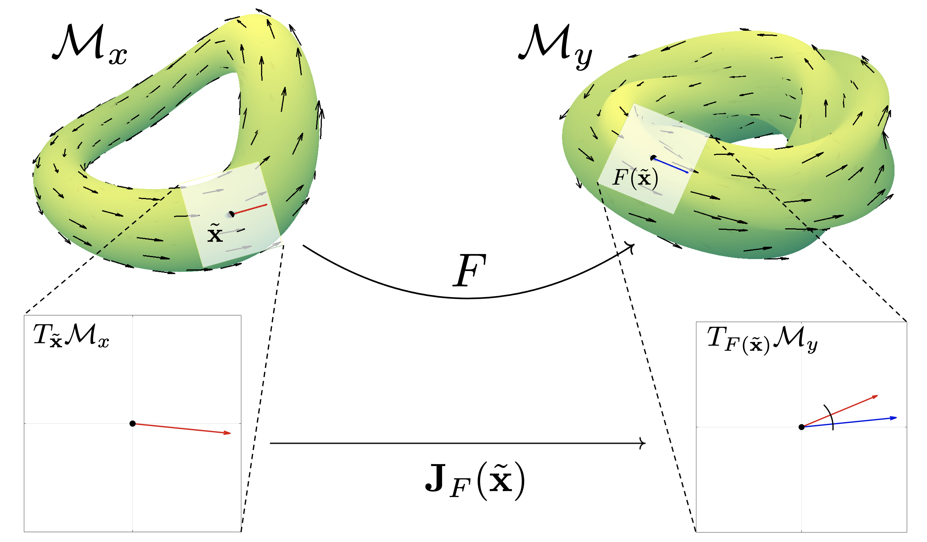
we may interpret to be a velocity vector field on the manifold. When evaluated, is a tangent vector of the manifold , existing in the tangent space 333See Appendix A for definitions of differential geometric quantities such as the tangent space.. From calculus, we know that tangent vectors in can be mapped to tangent vectors in by the Jacobian matrix at the point . By checking if the tangent vectors can be mapped in such a way, TSCI provides an alternative to the CCM causality test. A visual motivation for the TSCI methods is depicted in Fig. 1.
Before we can map vector fields from one manifold to another, we need to check that meaningful vector fields exist on the shadow manifolds. As usual, this is also a corollary of Takens’ theorem.
Corollary 2.1.2
There exists a vector field on such that the embedding in Takens’ theorem is a time-invariant mapping. If we define , and if we let to be the flow of a point under the vector field , then , for all times .
The proof of the corollary is provided in the Appendix.
The corollary guarantees that we can learn ODEs that describe the dynamics of and , once we have obtained valid reconstructions of the latent states. Let and be vector fields such that
| (9) | ||||
| (10) |
Because the cross map is a mapping between the two shadow manifolds, the Jacobian matrix of the cross map relates the vectors and . We state this formally in the following Lemma.
Lemma 2.1.1
Let and be manifolds with respective vector fields and that define their dynamics. If there exists a cross map , then for every point , we have that , where is the Jacobian matrix of at .
The proof of the lemma is in the Appendix.
While the cross map is a mapping between points on the manifolds, the Jacobian matrix induces a mapping between the tangent spaces at and . We show this visually in Fig. 1. Since the velocity of can be represented by a tangent vector , the Jacobian matrix allows us to map these vectors to tangent vectors in . If there is a cross map, then the vector field and the push forward vector field should match exactly. On the other hand, there should be no correlation in the absence of a causal relationship, assuming quality reconstructions and plentiful data. The degree of alignment between and can be used as a test statistic for the presence of a causal link. We therefore propose the TSCI test statistic,
| (11) |
Because the tangent vectors are centered in their respective tangent planes, we can geometrically interpret the TSCI test statistic as the expected cosine similarity between the vector field and the push forward vector field ,
| (12) |
In practice, the estimation quality of the cross map also depends on the location in the reconstruction space, and so the cosine similarity takes on a distribution of values (Fig. 2), and weak-to-moderate correlation may be empirically observed as an artifact of limited data.
Based on these analyses, we propose the TSCI method in Algorithm 1, which learns a cross-map and returns the alignment of the vector fields and . CCM is sensitive to the quality of the reconstruction of the latent states because an improperly constructed shadow manifold can sabotage the method, both theoretically and empirically [6]; TSCI similarly requires that the shadow manifold be properly embedded. Because of this, we assume that the embedding vectors and and the estimates of their vector fields and at each point are supplied as inputs to the algorithm. A variety of methods could be used to estimate the vector fields, but the simplest approach is to use finite differences,
where is the sampling rate of the data. Finite differences are known to be sensitive to noise, so in real scenarios a more careful approach to obtaining the time derivatives is necessary. For a practical implementation, we propose using the central finite-differences, which are second-order accurate [16], or the derivatives interpolated by a Savitsky-Golay filter for noisy data [34].
On methods to learn the cross map function. The TSCI algorithm is notably agnostic to the regression approach used for the cross map , with reasonable approaches including multilayer perceptron networks (MLPs), splines, and Gaussian process regression (GPR). Depending on the approach, derivatives can then be estimated from the model, either using automatic differentiation or analytical derivatives. For GPR in particular, analytical derivatives are straightforward to compute [38].
Since regression can sometimes be a computationally complex procedure, in Algorithm 2 we also provide a version of TSCI that is based on the -nearest regression, in analogy to CCM. For clean and dense data, this simple approach can yield accurate results, but it is generally unsuitable for noisy or sparse data. In the latter case, it is preferrable to combine the TSCI approach with other methods of denoising time series, or learning of latent dynamical models of the observed time series. In particular, the learning of a latent ODE learning [12] can be combined with the TSCI test to yield accurate causal inference.
On the use of correlation coefficient. In relation to CCM, it can be noted that both TSCI and CCM use a correlation coefficient as their test statistic. However, a critical difference between the two methods is how the usage of this statistic is justified. The correlation coefficient used in CCM analysis, called the cross-map skill [41], is used to measure the accuracy of predictions of the cross map. However, since the points being predicted in CCM live on a manifold, measuring correlation in the ambient (extrinsic) space is not well-motivated. Furthermore, estimates of this correlation can be biased by the distribution of observations along the manifold, and as a result, a high correlation can be achieved with a relatively low-accuracy prediction by guessing the general region in which the points lie.
In contrast, the correlation between tangent vectors (or vector fields) is a more geometrically motivated quantity: the correlation is a linear measure of similarity and the tangent vectors belong to a (centered) linear space. Additionally, the shadow manifolds are constructed to be submanifolds of Euclidean space, so correlations computed in extrinsic coordinates will match correlations computed using the intrinsic coordinates of the shadow manifold. By Lemma 2.1.1, the correlations will be identically if a cross map exists.
One alternative to the cosine similarity is the mutual information (MI). Specialized to the current text, the MI quantifies the reduction in the uncertainty of given the pushforward vector [9]. While the information-theoretic underpinning of the MI is attractive, we have two main reasons to prefer the cosine similarity: First, the MI between two (continuous) distributions can be difficult to interpret. For example, it is not obvious if is a strong dependence or not, particularly in the case of continuous distributions. The cosine similarity, on the other hand, is upper bounded by , so is easily interpreted as having near-perfect reconstruction. Second, accurate estimation of the MI from samples is a notoriously difficult task, particularly in high dimensions, and no single estimator works consistently well [10]. We provide some experiments with the MI, and show the differing performance of different estimators, in Section B.3.

3 Experiments
We validate the performance of TSCI on two datasets that are popular in the literature. The first arises from a coupled Rössler-Lorenz system, where the ground truth causality is known and the causal influence can be smoothly modulated. The second example was proposed in [12] and uses sporadic time series from coupled double pendulums, and illustrates the applicability of TSCI to extensions of CCM. Code implementing TSCI is available at https://github.com/KurtButler/tangentspaces. All comparisons to CCM use the skccm module in Python444https://github.com/nickc1/skccm, MIT License. Experiments were run on a 6-Core Intel Core i5 and NVIDIA Titan RTX.
3.1 Unidirectionally-Coupled Rössler-Lorenz System
A common toy system used for studying coupled dynamic systems is a unidirectionally-coupled Rössler-Lorenz system [28], which we define in Eq. 13. In this system, the first three coordinates () describe a Rössler system, and they are unidirectionally coupled with a Lorenz-type system (). The strength of the coupling is controlled by the parameter . When , the two systems are disconnected, but for there is a causal influence from to .
| (13) |
In Fig. 2, we visualize the TSCI method for and . First, we show the shadow manifolds and with a set of tangent vectors on each manifold. The delay embedding dimension parameters, and , were selected using the false-nearest neighbors algorithm with a tolerance of 0.005 [19].Time lags for the embeddings, and , were selected by picking the minimal delay such that the autocorrelation function drops below a threshold [21]. Additionally, we show the histograms of , where is the angle between the tangent vectors at each point. For direction, which is the true causal direction, the distribution is concentrated near 1. For the direction, the distribution of tangent vectors is centered on 0. The test statistics, and , correspond to the means of each distribution, and visibly correspond to the correct causality.
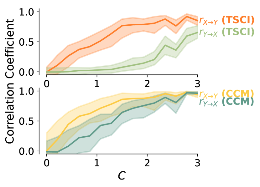
We show the effects of varying the coupling strength in Fig. 3(a), where TSCI clearly shows better separation across varying . We see the effect of increasing the library length (i.e., the size of the training set in nearest neighbors) for in Fig. 3(b). Here, increases at similar rates for TSCI and CCM, suggesting similar data efficiency of the two methods.

3.2 Double Pendulum System
To illustrate the generality of TSCI within CCM-like frameworks, we applied the TSCI methodology to the latent CCM framework, where CCM is applied to a state-space reconstruction obtained via neural ODEs [12]. One reason to favor this approach is when the observed time series are irregularly (i.e., with a non-uniform sampling rate) or sporadically (i.e., any given observation only measures a subset of states) sampled. Notable for TSCI is the fact that ground-truth derivatives are available, as they are directly learned in the neural ODE reconstruction.
We replicate an experiment in the latent CCM paper where a network of unidirectionally coupled double pendulums are simulated, and observations sampled irregularly and sporadically. The authors’ source code555https://github.com/edebrouwer/latentCCM, MIT License was used to generate data and apply latent CCM. For more information on the data generation, see Appendix A of [12].
For TSCI, we learn a cross-map using an MLP between the reconstructed state spaces. To avoid tuning learning rates for every network, the parameter-free COCOB optimizer [26]666https://github.com/bremen79/parameterfree, MIT License and networks were trained for epochs. Results can be found in Table 1.
| Direction | Latent CCM | Latent CCM (MLP) | Latent TSCI (MLP) |
|---|---|---|---|
When compared to latent CCM, TSCI provided larger correlation coefficients for the true positive cases, with similarly small coefficients for the true negative cases. The use of MLPs for learning the cross map partially but not fully explains the difference in performance.
3.3 Additional Experiments
Several additional experiments appear in Appendix B. We briefly describe them here and provide some commentary on their results.
Varying the Embedding Dimension
In Section B.1, we artificially lower quality embeddings by varying the embedding dimension. We find that the performance of TSCI and CCM similarly degrade when using an embedding dimension that is very small, and that there is little harm to a larger embedding dimension. In either case, the hyperparameters from a false-nearest neighbors test perform well.
Corrupting Signals
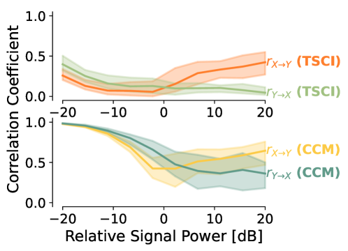
In Section B.2, we lower the embedding quality in two different ways: (1) by injecting additive noise to all observations, and (2) by adding a sine wave to observations. We observe that TSCI and CCM similarly degrade when the signal-to-noise ratio is altered. However, because of the larger separation in TSCI, the correct causal relation can be determined at much lower signal-to-noise ratios.
Using Mutual Information
In Section B.3, we experiment with using mutual information instead of cosine similarity. We find that conclusions made using MI are generally similar to those from cosine similarity, but with less interpretability and significant difficulties in estimation.
Comparisons to Other Causal Discovery Methods
As mentioned in the introduction, CCM (and hence TSCI) are specifically designed to address failures of Granger causality. In Section B.4, we empirically verify the limitations of Granger causality on our Rössler-Lorenz toy system. We additionally test several other causal discovery methods and show their limitations in our setting.
4 Advantages and Limitations of TSCI
Scalability. The TSCI approach, using the -nearest neighbors algorithm, retains the scalability and lightweight implementation that CCM enjoys. The only additional computational complexity arises from solving a local linear system of equations, and from the estimation of derivatives. Since the linear systems have a fixed size , and since derivative estimation can be done using a linear filter, the additional cost is minimal. The general version of TSCI will scale depending on the choice of the regressor used to learn the cross map, and on other design decisions made to improve the efficacy of the method. However, this is not unlike the situation in which CCM is augmented with other customization options that potentially slow down the method.
Model agnosticism. Because a TSCI test can be formulated for any differentiable regression model used to learn the cross map, the approach is highly flexible and model agnostic. Additionally, because there are many potential ways in which reconstruction of latent states and learning of the velocity vector fields can be improved, the TSCI method can be incorporated into a wide variety of inference frameworks.
Quality of reconstructed states. In both CCM and TSCI, there are a few assumptions which warrant some justification before use, since their violation may yield to misapplication of cross map methods. The first issue is that while Takens’ theorem implies that embeddings are plentiful, not all embeddings are equal in quality or useful. Shadow manifolds that are sparsely or incompletely sampled, time series with trends, or otherwise data which do not accurately capture the latent manifold can lead to dubious results using CCM [6]. While TSCI is less likely to produce a false positive in these cases, the assumption that a latent manifold is well-represented by a given embedding is nontrivial and critical to ensuring trustworthy performance of the method.
General synchrony. General synchrony is a problem that plagues all cross map-based methods [41]. The issue is that when the causal strength of the relationship is very strong, the influence of dominates the dynamics of , and cannot exhibit its own independent behavior. As a result, will look similar to , and the cross map will become an invertible function. As a result, a strong unidirectional relationship is detected as a bidirectional causal relationship. In Fig. 3, the Rössler-Lorenz system enters general synchrony near [6]. The TSCI method appears more resistant to the effects of general synchrony than CCM, but it is a topological fact that as grows, synchrony becomes inevitable.
5 Conclusion
In this paper, we presented the TSCI method for detecting causation in dynamical systems. By considering how tangent vectors map from one manifold to another, we may achieve more robust detection of causal relationships in dynamical systems than with standard CCM. Key advantages of TSCI include that we may use it in many systems in which CCM would be applied, but the method is far less prone to false positives and spurious causation. We presented both a general form of the algorithm as well as a -nearest neighbor version inspired by the original CCM algorithm. Because TSCI requires us to estimate latent states and their time derivatives, there us much room for the TSCI method to be further developed in future work.
Acknowledgments and Disclosure of Funding
We would like to thank the anonymous reviewers for their suggestions which improved the content and presentation of this work. This work was supported by the National Science Foundation under Award 2212506.
References
- [1] Kartik Ahuja, Divyat Mahajan, Yixin Wang, and Yoshua Bengio. Interventional causal representation learning. In International Conference on Machine Learning, pages 372–407. PMLR, 2023.
- [2] Jochen Arnhold, Peter Grassberger, Klaus Lehnertz, and Christian Erich Elger. A robust method for detecting interdependences: application to intracranially recorded EEG. Physica D: Nonlinear Phenomena, 134(4):419–430, 1999.
- [3] Zsigmond Benkő, Ádám Zlatniczki, Marcell Stippinger, Dániel Fabó, András Sólyom, Loránd Erőss, András Telcs, and Zoltán Somogyvári. Bayesian inference of causal relations between dynamical systems. Chaos, Solitons & Fractals, 185:115142, 2024.
- [4] Patrick Blöbaum, Dominik Janzing, Takashi Washio, Shohei Shimizu, and Bernhard Schölkopf. Cause-effect inference by comparing regression errors. In International Conference on Artificial Intelligence and Statistics, pages 900–909. PMLR, 2018.
- [5] Leo Breston, Eric J Leonardis, Laleh K Quinn, Michael Tolston, Janet Wiles, and Andrea A Chiba. Convergent cross sorting for estimating dynamic coupling. Scientific Reports, 11(1):20374, 2021.
- [6] Kurt Butler, Guanchao Feng, and Petar M Djurić. On causal discovery with convergent cross mapping. IEEE Transactions on Signal Processing, 2023.
- [7] Adam Thomas Clark, Hao Ye, Forest Isbell, Ethan R Deyle, Jane Cowles, G David Tilman, and George Sugihara. Spatial convergent cross mapping to detect causal relationships from short time series. Ecology, 96(5):1174–1181, 2015.
- [8] Sarah Cobey and Edward B Baskerville. Limits to causal inference with state-space reconstruction for infectious disease. PloS one, 11(12):e0169050, 2016.
- [9] Thomas M. Cover and Joy A. Thomas. Elements of Information Theory. Wiley-Interscience, USA, 2006.
- [10] Paweł Czyż, Frederic Grabowski, Julia E Vogt, Niko Beerenwinkel, and Alexander Marx. Beyond normal: On the evaluation of mutual information estimators. In Thirty-seventh Conference on Neural Information Processing Systems, 2023.
- [11] Povilas Daniušis, Dominik Janzing, Joris Mooij, Jakob Zscheischler, Bastian Steudel, Kun Zhang, and Bernhard Schölkopf. Inferring deterministic causal relations. In Proceedings of the Twenty-Sixth Conference on Uncertainty in Artificial Intelligence, pages 143–150, 2010.
- [12] Edward De Brouwer, Adam Arany, Jaak Simm, and Yves Moreau. Latent convergent cross mapping. In International Conference on Learning Representations, 2020.
- [13] Guanchao Feng, Kezi Yu, Yunlong Wang, Yilian Yuan, and Petar M Djurić. Improving convergent cross mapping for causal discovery with Gaussian processes. In 2020 IEEE International Conference on Acoustics, Speech and Signal Processing (ICASSP), pages 3692–3696. IEEE, 2020.
- [14] Bingbo Gao, Jianyu Yang, Ziyue Chen, George Sugihara, Manchun Li, Alfred Stein, Mei-Po Kwan, and Jinfeng Wang. Causal inference from cross-sectional earth system data with geographical convergent cross mapping. Nature Communications, 14(1):5875, 2023.
- [15] Clive WJ Granger. Investigating causal relations by econometric models and cross-spectral methods. Econometrica: Journal of the Econometric Society, pages 424–438, 1969.
- [16] Michael T Heath. Scientific Computing: An Introductory Survey. SIAM, 2018.
- [17] Patrik Hoyer, Dominik Janzing, Joris M Mooij, Jonas Peters, and Bernhard Schölkopf. Nonlinear causal discovery with additive noise models. Advances in Neural Information Processing Systems, 21, 2008.
- [18] Diviyan Kalainathan, Olivier Goudet, and Ritik Dutta. Causal discovery toolbox: Uncovering causal relationships in Python. Journal of Machine Learning Research, 21(37):1–5, 2020.
- [19] Matthew B Kennel, Reggie Brown, and Henry DI Abarbanel. Determining embedding dimension for phase-space reconstruction using a geometrical construction. Physical Review A, 45(6):3403, 1992.
- [20] Alexander Kraskov, Harald Stögbauer, and Peter Grassberger. Estimating mutual information. Physical Review E, 69(6):066138, 2004.
- [21] Dimitris Kugiumtzis. State space reconstruction parameters in the analysis of chaotic time series—the role of the time window length. Physica D: Nonlinear Phenomena, 95(1):13–28, 1996.
- [22] John M Lee. Introduction to Smooth Manifolds, volume 218 of Graduate Texts in Mathematics. Springer, second edition, 2012.
- [23] Huanfei Ma, Kazuyuki Aihara, and Luonan Chen. Detecting causality from nonlinear dynamics with short-term time series. Scientific Reports, 4(1):7464, 2014.
- [24] A. McInerney. First Steps in Differential Geometry: Riemannian, Contact, Symplectic. Undergraduate Texts in Mathematics. Springer New York, 2013.
- [25] Dan Mønster, Riccardo Fusaroli, Kristian Tylén, Andreas Roepstorff, and Jacob F Sherson. Causal inference from noisy time-series data—testing the convergent cross-mapping algorithm in the presence of noise and external influence. Future Generation Computer Systems, 73:52–62, 2017.
- [26] Francesco Orabona and Tatiana Tommasi. Training deep networks without learning rates through coin betting. Advances in Neural Information Processing Systems, 30, 2017.
- [27] Judea Pearl. Causality. Cambridge University Press, 2009.
- [28] R Quian Quiroga, Jochen Arnhold, and Peter Grassberger. Learning driver-response relationships from synchronization patterns. Physical Review E, 61(5):5142, 2000.
- [29] Nikolai F Rulkov, Mikhail M Sushchik, Lev S Tsimring, and Henry DI Abarbanel. Generalized synchronization of chaos in directionally coupled chaotic systems. Physical Review E, 51(2):980, 1995.
- [30] Jakob Runge, Andreas Gerhardus, Gherardo Varando, Veronika Eyring, and Gustau Camps-Valls. Causal inference for time series. Nature Reviews Earth & Environment, 4(7):487–505, 2023.
- [31] Jakob Runge, Vladimir Petoukhov, Jonathan F Donges, Jaroslav Hlinka, Nikola Jajcay, Martin Vejmelka, David Hartman, Norbert Marwan, Milan Paluš, and Jürgen Kurths. Identifying causal gateways and mediators in complex spatio-temporal systems. Nature Communications, 6(1):8502, 2015.
- [32] Tim Sauer. Reconstruction of dynamical systems from interspike intervals. Physical Review Letters, 72(24):3811, 1994.
- [33] Tim Sauer, James A Yorke, and Martin Casdagli. Embedology. Journal of Statistical Physics, 65:579–616, 1991.
- [34] Abraham Savitzky and Marcel JE Golay. Smoothing and differentiation of data by simplified least squares procedures. Analytical Chemistry, 36(8):1627–1639, 1964.
- [35] Steven J Schiff, Paul So, Taeun Chang, Robert E Burke, and Tim Sauer. Detecting dynamical interdependence and generalized synchrony through mutual prediction in a neural ensemble. Physical Review E, 54(6):6708, 1996.
- [36] Bernhard Schölkopf, Francesco Locatello, Stefan Bauer, Nan Rosemary Ke, Nal Kalchbrenner, Anirudh Goyal, and Yoshua Bengio. Toward causal representation learning. Proceedings of the IEEE, 109(5):612–634, 2021.
- [37] Skipper Seabold and Josef Perktold. statsmodels: Econometric and statistical modeling with Python. In 9th Python in Science Conference, 2010.
- [38] Ercan Solak, Roderick Murray-Smith, WE Leithead, Douglas Leith, and Carl Rasmussen. Derivative observations in Gaussian process models of dynamic systems. Advances in Neural Information Processing Systems, 15, 2002.
- [39] Jaroslav Stark. Delay embeddings for forced systems. I. Deterministic forcing. Journal of Nonlinear Science, 9:255–332, 1999.
- [40] Jaroslav Stark, David S Broomhead, Michael Evan Davies, and J Huke. Delay embeddings for forced systems. II. Stochastic forcing. Journal of Nonlinear Science, 13:519–577, 2003.
- [41] George Sugihara, Robert May, Hao Ye, Chih-hao Hsieh, Ethan Deyle, Michael Fogarty, and Stephan Munch. Detecting causality in complex ecosystems. Science, 338(6106):496–500, 2012.
- [42] Floris Takens. Detecting strange attractors in turbulence. In David Rand and Lai-Sang Young, editors, Dynamical Systems and Turbulence, Warwick 1980, pages 366–381, Berlin, Heidelberg, 1981. Springer.
- [43] Gherardo Varando, Miguel-Ángel Fernández-Torres, Jordi Muñoz-Marí, and Gustau Camps-Valls. Learning causal representations with Granger PCA. In UAI 2022 Workshop on Causal Representation Learning, 2022.
- [44] Hao Ye, Ethan R Deyle, Luis J Gilarranz, and George Sugihara. Distinguishing time-delayed causal interactions using convergent cross mapping. Scientific Reports, 5(1):14750, 2015.
- [45] Hao Ye and George Sugihara. Information leverage in interconnected ecosystems: Overcoming the curse of dimensionality. Science, 353(6302):922–925, 2016.
- [46] Yujia Zheng, Biwei Huang, Wei Chen, Joseph Ramsey, Mingming Gong, Ruichu Cai, Shohei Shimizu, Peter Spirtes, and Kun Zhang. Causal-learn: Causal discovery in Python. Journal of Machine Learning Research, 25(60):1–8, 2024.
Appendix A Important Facts About Manifolds
In this appendix, we review some important background about manifolds. Much more complete references include the authoritative [22] (especially chapters 1, 2, 3, and 8), or the more accessible [24].
We say that a function is smooth if it has derivatives of all orders. A diffeomorphism is a function which is smooth, invertible, and is also smooth. We say that two subsets and of are diffeomorphic if there exists a diffeomorphism such that .
A subset of is called a -dimensional manifold if for every point in , there exists an open set such that
-
1.
There is a diffeomorphism .
-
2.
The image of the set under is given by
Without a loss of generality, we can assume that in this definition. This allows us to easily define tangent vectors. A vector is called a tangent vector of at the point if there exists a path in such that
where is the diffeomorphism in the above definition. The tangent space is defined to be the set of all tangent vectors of at . Note that from these definitions, it is clear that is a manifold and .
In calculus, we define a vector field on to be a function . We generalize this to manifolds in Euclidean space by defining a vector field on to be a mapping such that at every point .
An embedding of a manifold is a mapping such that restricted to is a diffeomorphism onto its image. If is a manifold of dimension and is an embedding, then is necessarily greater than or equal to . In general, it is an interesting question to ask how much larger must be so that embeddings are easy to find. The Whitney embedding theorem says that it is a generic property that when . Takens’ theorem refines the Whitney theorem by asserting that such an embedding can be obtained from a scalar observation function, by time lagging the observations sufficiently many times.
Appendix B Additional Experiments
In this appendix, we include experiments and results omitted from the main text.
B.1 Varying Embedding Dimension
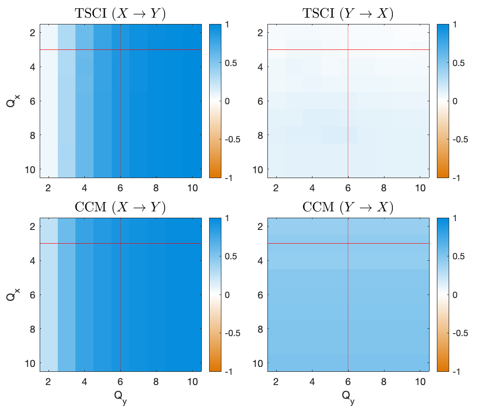
One of the key parameters in both CCM an TSCI is the embedding dimension parameter used during reconstruction of the shadow manifold. Takens’ theorem suggests that once reaches a certain value, the manifold is embedded and the improvement of the results should saturate in principle. Of course, in real life there is a curse of dimensionality associated with inference, so it is interesting to check how well the results behave as the embedding dimension is chosen to be higher than necessary. We consider the effect of varying the parameter using data from the Rössler-Lorenz system in Fig. 4. Performance of both methods improve as the dimension of the putative effect (if we are testing , then this is ) is increased, until saturating after the manifolds are fully embedded.
B.2 Corrupted Signals
Generally, there are many non-trivial ways in which the state reconstruction can be poor, e.g., presence of periodic trends [8] and underexploration of the shadow manifold [6]. We consider two scenarios that deteriorate the state reconstruction quality on the Rössler-Lorenz system: additive noise, and a periodic trend.
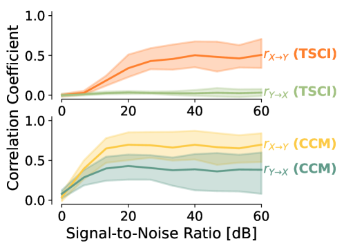
Results for additive noise are presented in Fig. 5. We fixed and varied the signal-to-noise ratio (SNR) from dB to dB by adding Gaussian noise to the observed signals. When estimating derivatives, a Savitzky-Golay filter [34] was used with a window length of and order .
Overall, we find the performance relative to SNR to be similar between CCM and TSCI, suggesting that inference of the vector field from noisy data is not a limiting factor in the presence of additive noise.
An alternative way to corrupt signals is with a deterministic periodic trend; we used a sine wave with a period of , and varied its power with respect to the true signal. Results are presented in Fig. 6. Our takeaways are relatively similar to the additive noise experiment: TSCI seems to degrade similarly to CCM, but its increased separation between cause and effect makes this degradation in performance less problematic. Notably, TSCI seems significantly more robust to false claims of strong causation when the relative power of the confounder is large.
B.3 Using the Mutual Information for Scores
One interesting alternative to the cosine similarity score is the mutual information (MI), which provides a non-linear quantification of how related and are. One immediate concern with using MI is that estimates from finite samples are difficult; we use the classical estimator of Kraskov, Stögbauer, and Grassberger [20], which has shown relevance even in the era of deep learning [10].
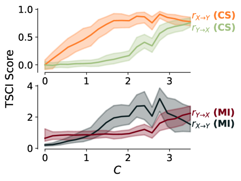
Results on the Rössler-Lorenz test system while varying the coupling parameter are presented in Fig. 7. We find that MI typically shows less separation than TSCI, which brings into question its viability when the ground truth is unknown. Another issue is in the interpretation of MI estimates: it is not entirely clear if an MI estimate of, for example, nat indicates strong influence, and MI estimates are not easily normalized in the continuous setting.
B.4 Comparisons to Other Causal Discovery Methods
As argued in the main manuscript, cross-map-based methods such as TSCI and CCM approach causal discovery in a rather particular setting, where more mainstream methods do not apply. We empirically verify these claims on the Rössler-Lorenz test system, using a variety of values of . We compare against Granger causality, as well as various bivariate causal discovery methods.
We first compare against Granger causality in Table 2. As expected from the theory, Granger causality incorrectly infers bidirectional causality for all .
We also compare against various methods from the bivariate or pairwise causal discovery literature. These methods typically assume the existence of a map which is either deterministic or subject to additive noise, which does not exist in all but the most trivial dynamical systems. This includes RECI [4], IGCI [11], and ANM [17]. Results are presented in Tables 3 and 4.
We find that IGCI consistently fails to detect a causal edge, with weak coefficients. RECI consistently chooses the direction , but does so even when , which suggests that results are not actually detecting causality, but rather some other anomaly of the data. To this end, the variance ratios as described by Blobaum et al. [4] are typically large, indicating little confidence. Finally, for all , ANM detects bidirectional causality.
Comparisons with Granger causality use the implementation of statsmodels777https://github.com/statsmodels/statsmodels/, BSD-3-Clause License [37]. All comparisons to RECI and IGCI used the implementations of cdt888https://github.com/FenTechSolutions/CausalDiscoveryToolbox, MIT License [18], with a minor bug-fix for RECI. Comparisons with ANM used the implementation of causal-learn999https://github.com/py-why/causal-learn, MIT License [46].
| p-value | p-value | |
|---|---|---|
| RECI | IGCI | |
|---|---|---|
Appendix C Proofs
In this section, we provide proofs for results mentioned in the main text.
Proof of Theorem 2.1
Proof of Corollary 2.1.1
Let us assume that we have a generic system, where for some manifold , and is a function and is a function of .
If and both hold, then and are both diffeomorphic to , and thus, diffeomorphic to each other. The existence of a cross map is then immediate.
If but not vice-versa, then the dynamics of are autonomous, meaning that the behavior of depends only upon itself. As a result, the projection map can be applied directly to to yield a new manifold on which is an autonomous dynamical system. Since observes this system , will be diffeomorphic to , since only contains information about . Let and denote the diffeomorphisms implied by Takens’ theorem. We can construct the cross map then as
Proof of Corollary 2.1.2
Since the shadow manifold produced by Takens’ theorem is a smooth embedding of the original manifold , there exists a diffeomorphism . By Proposition 8.19 of Lee [22, p. 183], for any given vector field defined on , there exists a unique vector field on that is the push forward of under the map . Because the dynamics on the manifold are derived from these vector fields, the two systems are equivalent as dynamical systems.
Proof of Lemma 2.1.1
Suppose that is a cross map. Fix any point and let . If we consider flows forwards and backwards with respect to these vector fields, then there exists some small such that we have curves along and along such that for each in the interval . By the chain rule of calculus, we have that
where is the Jacobian matrix of the function at the point . Since the dynamics of these spaces are given by vector fields, we can replace the time derivatives in the equation with their vector fields:
Since the point that we chose was arbitrary, the statement holds for every point in .