pacer: Preference-conditioned All-terrain
Costmap Generation

Abstract

In autonomous robot navigation, terrain cost assignment is typically performed using a semantics-based paradigm in which terrain is first labeled using a pre-trained semantic classifier and costs are then assigned according to a user-defined mapping between label and cost. While this approach is rapidly adaptable to changing user preferences, only preferences over the types of terrain that are already known by the semantic classifier can be expressed. In this paper, we hypothesize that a machine-learning-based alternative to the semantics-based paradigm above will allow for rapid cost assignment adaptation to preferences expressed over new terrains at deployment time without the need for additional training. To investigate this hypothesis, we introduce and study pacer, a novel approach to costmap generation that accepts as input a single birds-eye view (BEV) image of the surrounding area along with a user-specified preference context and generates a corresponding BEV costmap that aligns with the preference context. Using both real and synthetic data along with a combination of proposed training tasks, we find that pacer is able to adapt quickly to new user preferences while also exhibiting better generalization to novel terrains compared to both semantics-based and representation-learning approaches.

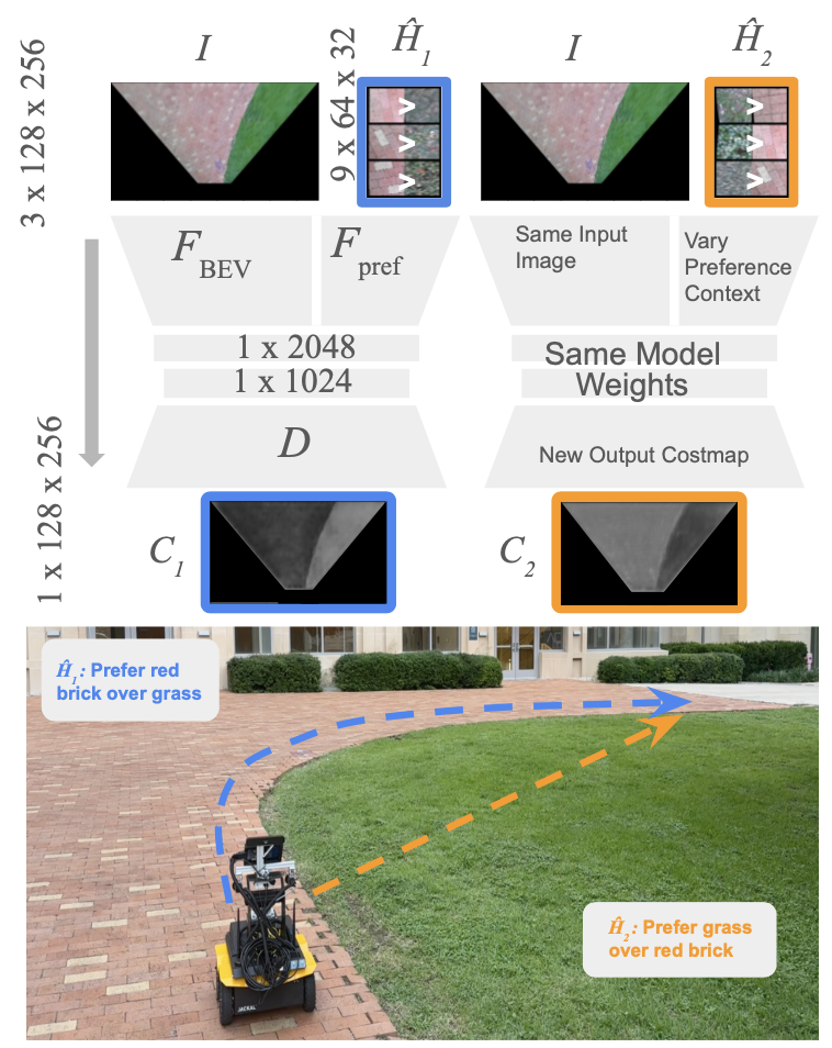
Figure 1: Given an input image $I$ and a preference context $\hat{H{}}$ of $n$ ordered pairs of terrain patches where the left terrain is more preferred than the right, pacer generates a costmap consistent with this preference. Changing the preference context leads to changed terrain costs, which results in a different plan aligned to the new operator preference. The paths planned according to the different preferences are shown above.

I Introduction and Related Work

Robust and aligned autonomous ground vehicle navigation in a wide variety of environments is a long-standing goal in the robotics community. While there has been progress on the classical problem of collision-free waypoint navigation in static, simple environments [1][2], there are still significant challenges in constructing autonomous systems that can navigate in environments that are dynamic, more complex, or both [3]. Further, successful operation in such environments typically relies on robots understanding and aligning their behaviors to specified human preferences for navigation that go beyond simple waypoint achievement, e.g., preferring to cross a busy street at a crosswalk even if doing so results in a longer path to a waypoint [4][5].

In this paper, we consider the specific question of how robots should assign costs to terrain such that those costs align with human preferences for terrain traversal. Having robots adhere to preferences of this type is useful both for helping enable robust navigation in complex environments and also for ensuring that robots adhere to other constraints such as social norms [6] [7]. While seeking to assign appropriate costs to terrain is not the only way to ensure aligned navigation behavior (e.g., one may instead seek navigation control policies that are aligned to human preferences [8][9][10]), we choose to focus on assigning terrain costs here due to its prevalence in the existing literature, as many existing and well-understood autonomous planning frameworks leverage costmaps to produce cost-optimal behaviors [11] [12] [13].

We are particularly interested here in terrain cost assignment approaches that can rapidly adapt to newly-expressed terrain preferences. Popular approaches such as inverse reinforcement learning (IRL) and preference-based IRL (PbIRL) based on terrain patch clusters do not admit this type of rapid adaptation due to the amount of additional data required to express or query for the new preference [14] [15] [16]. Instead, to the best of our knowledge, the most commonly-employed systems with this capability follow a semantics-based paradigm in which the surrounding terrain is first labeled using a pre-trained semantic classifier and human preferences are conveyed via a manually specified label-to-cost mapping [5] [17][18]. Such systems exhibit rapid adaptation to new preferences by design: the new costmaps can be generated as soon as the user provides a new label-to-cost mapping, which is typically accomplished in seconds to minutes. However, these systems are also inherently limited in that the user can only specify preferences with respect to the terrain types known to the classifier.

Another class of methods designed for terrain-aware aware navigation is by representing terrains as vectors in a continuous embedding space, so preference are no no longer limited to terrains with predefined labels [14] [19] [20]. Patch-based representation learning methods for terrain understanding typically involve mapping small square patches from the bird’s-eye view (BEV) to a representation vector that is further converted into a scalar cost value.

Although continuous representation spaces are theoretically generalizable to new terrains, training such a space effectively is challenging in practice, since even humans may struggle to identify terrain types from small patches in the presence of homography artifacts or difficult lighting conditions. A further limitation is that each new preference ordering over terrains necessitates retraining the utility function in the representation space, making these approaches less adaptable to changing operator preferences.

Towards overcoming the limitations of the semantics-based and representation-learning paradigms to terrain cost assignment, we propose and study pacer, a novel approach to costmap generation that accepts as input a single birds-eye view (BEV) image of the surrounding terrain along with a user-specified preference context and generates a corresponding BEV cost map that aligns with that preference context (see Fig. 1). By preference context, we mean a small set of terrain patches and pairwise preferences over those patches that are supplied at deployment time. We design pacer to exhibit three design desiderata: (1) it is capable of representing a prior over terrain preferences; (2) it is capable of adapting to a wide variety of preference contexts; and (3) it is able to assign aligned costs to terrains that appear in both the preference context and the BEV image, even for novel terrain types.

Using real and synthetic terrain data, we implement a training pipeline to realize these three properties and evaluate the resulting preference-conditioned costmap functions over a wide variety of BEV images. Additionally, we study the impact of the resulting costmaps on cost-optimal navigation behavior with respect to adherence to human preferences. We find that our method overcomes limitations in prior works by being easily adaptable to new operator preferences and producing fine-grained costmaps that illicit desirable navigation behaviors even in previously unseen environments.

II The Terrain-Aware Preference-Aligned Planning Problem

Figure 2: Relationships between spaces of Terrains, Image Observations, and Costmaps. There exists a hidden “true” costing function based on human preferences directly on terrains. pacer approximates this function from visual observations of terrains.

We now develop the terrain-aware preference-aligned planning problem. We will first formulate the path planning problem, and then we will discuss the problem of learning preference-aligned terrain costs.

II-A Path Planning

In this paper, we are concerned with the general problem of planning a path in a robot state space $\mathcal{X}{}$ ($\mathrm{SE}(2)$ for ground vehicles) from a start and goal pose $x{}_{1},G\in\mathcal{X}{}$ as the problem of finding the finite trajectory $\Gamma_{S}=[x{}_{1},...,x_{S}]$ consisting of $S$ states $x{}\in\mathcal{X}{}$ which minimizes a total objective function

$$\Gamma_{S}=\arg_{\Gamma}\min||x{}_{S}-G||+\lambda\mathcal{J}(\Gamma),$$ (1)

where $||x{}_{S}-G||$ is the distance between the final state $x{}_{S}$ and $G$, and $\mathcal{J}(\Gamma)$ is the cost function scaled by the relative weight $\lambda$.

A cost function $\mathcal{J}(\Gamma)$ may include various terms such as the geometric cost of obstacles, social navigation cost, or terrain cost,

$$\mathcal{J}(\Gamma)=\mathcal{J}_{\text{geometric}}(\Gamma)+\alpha\mathcal{J}_{\text{social}}(\Gamma)+\beta\mathcal{J}_{\text{terrain}}(\Gamma)$$ (2)

where $\alpha,\beta$ are relative weights. This paper is concerned with the terrain cost term $\mathcal{J}_{\text{terrain}}(\Gamma)$ of the general function.

II-B Preference-Aligned Terrain Costs

To better understand preference-aligned terrain costs, we first introduce a fixed terrain function to represent the spatial distribution of the terrains in the world. Let a terrain map $T:\mathcal{X}{}\rightarrow\mathcal{T}{}$ be a function that maps a robot pose $x\in\mathcal{X}$ to the terrain $\tau\in\mathcal{T}$ that the robot interacts with when in pose $x$, where a terrain $\tau$ captures all the properties of the ground relevant to robot navigation.

Additionally, we assume the human has an unknown true cost function $H{}:\mathcal{T}{}\rightarrow\mathbb{R}^{0+}$ mapping terrains to scalar real-valued costs based on their preferences. This cost function is influenced by various factors, including the personal preferences of human operator, the environment, and the task at hand. Let $\mathcal{H}$ denote the continuous space of such cost functions, such that $H{}\in\mathcal{H}{}$.

For terrain-aware navigation, the robot relies on its visual observations to infer terrain-specific costs. We assume that these observations arrive in the form of images generated according to a black-box observation function $O{}:\mathcal{X}{}\times\mathbb{T}{}\to\mathcal{I}{}$, i.e., $I=O(x,T)$, where $x$ is the observing pose of the robot, $T$ is a terrain map, $\mathbb{T}$ is the space of terrain maps, and $\mathcal{I}$ is the space of images. In practice, most methods operate on synthetic birds-eye-views generated from the original camera images. BEV images can be generated via static ground-plane homography [15][14], or a BEV accumulation algorithm [21]. Henceforth, we define input images to be BEV images. We assume that the the visual appearance of the terrain provides sufficient information for the robot to perform terrain-aware navigation. The observation function is thus fixed, but unknown to the robot.

During planning, the terrain cost of a pose is found using a costmap $C{}:\mathcal{X}{}\to\mathcal{R}^{0+}$ that maps from robot poses to costs. We introduce a costmap generation function $R{}:\mathcal{I}{}\times\mathcal{H}{}\to\mathcal{C}{}$ as the function mapping from the space of images $\mathcal{I}$ to the space of costmaps $\mathcal{C}$, conditioned on an unknown human cost function that belongs to $\mathcal{H}$.

Since the robot has no direct access to the terrain map $T{}$ and there is no clear representation of $H{}$, the terrain-aware preference-aligned planning problem is thus to learn the function $R$ such that, given an image observation of terrain, the optimal trajectory planned with respect to $R$ is also optimal with respect $H$. The conditions in the next section will be introduced as our analyses of how we address this problem.

III Necessary Conditions for Preference-Aligned Navigation

Seeking training tasks that will help us compute valid preference-conditioned costmap functions $R(\cdot|H)$, we now state a set of conditions that are necessary for these tasks to produce costmaps that are consistent with human preferences for terrain.

In particular, we will state conditions for equivalence, partial ordering, and viewpoint invariance, and we will show that $R$s that produce costmaps that yield optimal trajectories consistent with a human preference must obey these conditions.

Let $R{}(\cdot|H{})$ denote a costmap generated according to an $H{}\in\mathcal{H}{}$, and $C{}|_{x}{}$ denote that costmap $C{}\in\mathcal{C}{}$ is evaluated at pose $x$. For a generated costmap $R{}(\cdot|H{})$ to be consistent with $H{}$

, we specify it must exhibit both equivalence and partial ordering. By equivalence, we mean that the terrains at two poses are given the same cost by $H$ if and only if the costmap generated by $R$ from an image observation and evaluated at those two poses have equal cost, i.e.,

$$H{}_{i}(T(x_{1})) =H{}_{i}(T(x_{2}))\iff R{}(O{}(\cdot,T)\mid H{}_{i})\Big{|}_{x_{1}}$$

$$=R{}(O{}(\cdot,T)\mid H{}_{i})\Big{|}_{x_{2}}\quad\forall x_{1},x_{2},H{}_{i}\;.$$ (NC1)

By partial ordering, we mean that $H$ assigns a preference order over the terrains at two poses if and only if the costmap generated by $R$ from an image observation assigns those two poses the same preference order, i.e.,

$$H{}_{i}(T(x_{1})) <H{}_{i}(T(x_{2}))\iff R{}(O{}(\cdot,T)\mid H{}_{i})\Big{|}_{x_{1}}$$

$$<R{}(O{}(\cdot,T)\mid H{}_{i})\Big{|}_{x_{2}}\quad\forall x_{1},x_{2},H{}_{i}\;.$$ (NC2)

We let $O(\cdot,T)$ denote an image observation captured from any observing pose from which $x_{1},x_{2}$ are visible.

We now provide a brief proof that NC1 NC2 are necessary for aligning the preferences of $H{}_{i}$ with $R{}$. Specifically, if the most optimal path with respect to $R{}(\cdot\mid H{}_{i})$ has the same optimal cost when evaluated with $H{}_{i}$, then the conditions (NC1) and (NC2) must hold. For a trajectory $\Gamma$ composed of discrete poses, let the cumulative cost function for the human’s evaluation be denoted by $H{}|_{\Gamma}\equiv\sum_{x_{i}\in\Gamma}H{}(T(x{}_{i}))$. Similarly, let the cumulative cost function based on the generated costmap be denoted as $R{}|_{\Gamma}\equiv\sum_{x_{i}\in\Gamma}R{}(O{}(\cdot,T)\mid H{})|_{x_{i}}$. Given this setup, the following theorem establishes the necessity of the conditions (NC1) and (NC2) such that $H{}|_{\Gamma^{\ast}}=R{}|_{\overline{\Gamma}}$.

Theorem 1.

Let $\Gamma^{\ast}=\arg_{\Gamma}\min H{}|_{\Gamma},\quad\overline{\Gamma}=\arg_{\Gamma}\min R{}|_{\Gamma}$ denote the optimal trajectories with respect to $H{}$ and $R{}$ respectively. If the optimal trajectory with respect to $R$ has equal cost to the optimal path with respect to $H$ when both are evaluated on $H$ such that $H{}|_{\Gamma^{\ast}}=R{}|_{\overline{\Gamma}}$, then conditions (NC1) and (NC2) hold.

Proof.

Since $H{}|_{\Gamma^{\ast}}=R{}|_{\overline{\Gamma}}$, we must have that:

1. $H{}|_{\Gamma_{1}}<H{}|_{\Gamma_{2}}\Rightarrow R{}|_{\Gamma_{1}}<R{}|_{\Gamma_{2}}$ for all paths $\Gamma_{1},\Gamma_{2}$.

   Otherwise, there exist paths $\Gamma_{1},\Gamma_{2}$ such that $H{}|_{\Gamma_{1}}<H{}|_{\Gamma_{2}}$ and $R{}|_{\Gamma_{1}}\geq R{}|_{\Gamma_{2}}$. Then, $\Gamma_{2}$ may be selected as $\overline{\Gamma}$, but has greater cost than $H{}|_{\Gamma^{\ast}}$ when evaluated on $H$, which is a contradiction.

2. $R{}|_{\Gamma_{1}}<R{}|_{\Gamma_{2}}\Rightarrow H{}|_{\Gamma_{1}}<H{}|_{\Gamma_{2}}$ for all paths $\Gamma_{1},\Gamma_{2}$.

   Otherwise, there exist paths $\Gamma_{1},\Gamma_{2}$ such that $R{}|_{\Gamma_{1}}<R{}|_{\Gamma_{2}}$ and $H{}|_{\Gamma_{1}}>H{}|_{\Gamma_{2}}$ (by contraposition on (a), we eliminate the case where $R{}|_{\Gamma_{1}}<R{}|_{\Gamma_{2}}$ and $H{}|_{\Gamma_{1}}=H{}|_{\Gamma_{2}}$). Then, $\Gamma_{1}$ may be selected as $\overline{\Gamma}$, but may have greater cost than $H{}|_{\Gamma^{\ast}}$ when evaluated on $H$, which is a contradiction.

By (a) and (b), we have that $H{}|_{\Gamma_{1}}<H{}|_{\Gamma_{2}}\iff R{}|_{\Gamma_{1}}<R{}|_{\Gamma_{2}}$. By contraposition, we also have $H{}|_{\Gamma_{1}}=H{}|_{\Gamma_{2}}\iff R{}|_{\Gamma_{1}}=R{}|_{\Gamma_{2}}$. Finally, since a path $\Gamma$ can consist of a single state, conditions (NC1) and (NC2) must also then hold. ∎

In the next section, we use conditions (NC1) and (NC2) to define training tasks for learning the optimal $R$ from data, which drives our proposed approach to the online generation of costmaps which result in preference-aligned navigation.

IV Preference-Aligned All-Terrain Costmap Generation

We now present our proposed approach for computing aligned terrain costmaps, which we refer to as Preference-aligned, All-terrain Costmap genERation (pacer). pacer introduces the notion of a preference context and comprises several components, including a neural network architecture, and a data curation and training methodology based on the three design desiderata.

IV-A Preference Context

The preference-aligned terrain costs discussed in Section II depend on a human’s cost function $H:\mathcal{T}\rightarrow\mathbb{R}^{0+}$. Unfortunately, we do not have access to $H$ directly since it is known only to the human operator. Therefore, we propose to obtain and utilize an approximate representation of $H$ that we call a preference context.

We define a preference context $\hat{H{}}$ as a set of $n$ image patch pairs $\widetilde{I{}}\succ\widetilde{I{}}^{\prime}$ constructed from human input

such that the human prefers the terrain observed in image $\widetilde{I{}}$ over the terrain observed in $\widetilde{I{}}^{\prime}$, where an $\widetilde{I{}}\in\mathcal{I}{}$ is an observation of terrain as a small image patch. The small patch may be a part of a larger bird’s-eye-view image of the ground.

More specifically, $\hat{H{}}$ consists of $n$ preferences derived from $H{}$ and is defined as $\hat{H{}}\equiv\{(\widetilde{I{}}_{1}\succ\widetilde{I{}}_{1}^{\prime}),...(\widetilde{I{}}_{n}\succ\widetilde{I{}}_{n}^{\prime})\}$. Fig 3 shows some example preference contexts with $n=3$ patch pairs and their corresponding costmaps.

In our implementation, the $n$ pairwise preferences are expressed using image patches of size $w\times h$. $\hat{H{}}$ is then represented by vertically concatenating the patches within a pair with the more-preferred terrain patch on top and forming a single $n\times c\times w\times 2h$ tensor, where $c$ is the number of color channels.

IV-B Model Architecture

To generate costmaps, we propose to approximate functions $R:\mathcal{I}\times\mathcal{H}\rightarrow\mathcal{C}$, which require $H$ as input, with functions $\hat{R}:\mathcal{I}\times\hat{\mathcal{H}}\rightarrow\mathcal{C}$, where $\hat{\mathcal{H}}$ is the space of all preference contexts as defined above. We model $\hat{R}$ as a neural network with a two encoders and a single decoder. The input image is passed through a BEV image encoder $F_{\mathrm{BEV}}$ to form an image embedding, and, similarly, the input preference context is passed through a preference context encoder $F_{\mathrm{pref}}$ to form a preference embedding. The output costmap is then generated by concatenating these embeddings and then passing them through a decoder $D$. A visual depiction of this architecture is provided in Fig. 1.

IV-C Loss Function

pacer is trained using supervised machine learning, i.e., given a dataset $\mathcal{D}=\{(\hat{H},I{},C{}_{T})_{i}\}_{i=1}^{N}$ of preference context, image, and target costmap tuples, we seek the parameters $\phi$ of $\hat{R}$ that minimize a loss between the real and predicted costmaps. More specifically, we seek $\phi^{\ast}$ such that

$$\phi^{\ast}=\arg\min_{\phi}\mathbb{E}_{(I,\hat{H},C_{T})\sim\mathcal{D}}\left[\ell\left(\hat{R}_{\phi}(I,\hat{H}),C_{T}\right)\right]\;,$$ (3)

where we use the binary cross entropy loss averaged over each pixel as the loss function $\ell$.

V Dataset Curation and Training pacer

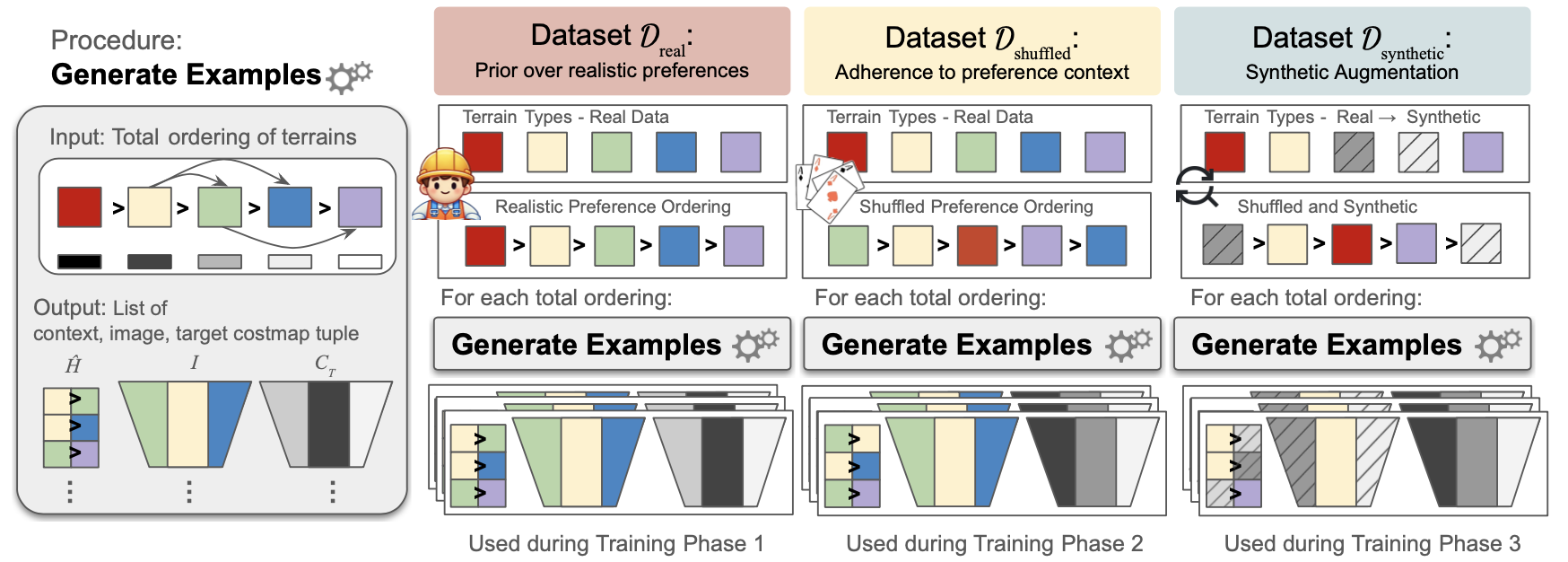
Figure 3: Overview of the dataset structure. Each training example contains a preference context, image, and target costmap. We vary the preferences and images, resulting in a large combinatorial dataset despite the relatively small amount of real recorded data. In a later training phase, we also augment with synthetic data by artificially finding and replacing certain terrain types with synthetic terrain textures. The real-valued costs assigned to terrain types based on an input total ordering are shown in the Generate Examples procedure, where black represents low cost and white is high cost.

We now describe the dataset curation and training process for pacer. pacer is trained using three distinct phases of supervised machine learning, each corresponding to a unique training dataset that corresponds to one of the desiderata desecribed in Section I. In what follows, we will first describe how we generate training examples, then describe each of the three training phases and the training procedure.

V-A Training Example Generation

The datasets $\mathcal{D}$ we use to train the pacer model consist of tuples of preference contexts, images, and target costmaps $(\hat{H},I,C_{T})$. To construct these datasets, we bootstrap off of semantic terrain classification and use a pretrained terrain patch classifier that assigns one of $L$ predefined semantic labels to a given terrain image patch.

The inputs to the training example generation process are a single image $I$ along with a total ordering over terrain types $\tau_{1}\succ\tau_{2}\succ\ldots\succ\tau_{L}$, where each terrain type $\tau_{l}$ corresponds to a bank of image patches. pacer assumes that the cost value associated with $\tau_{l}$ is given by $H{}(\tau_{l})=\frac{l-1}{L-1}$. The patch bank that corresponds to $\tau_{l}$ consists of patches of that type that have been extracted from images collected during robot deployment.

We use these inputs to generate $\hat{H{}}$ and $C{}_{T}$. To generate $\hat{H{}}$, we first choose $n$ ordered pairs from the total ordering over the $L$ terrain types without replacement. For each of the resulting ordered pairs, we sample uniformly at random patches from the corresponding patch banks, and use these $2n$ patches to construct $\hat{H{}}$ according to the process detailed in Section IV-A above. To generate $C{}_{T}$, we first perform semantic segmentation on $I$ and then transform the segmented image into $C_{T}$ by setting the cost for a pixel labelled $l$ to be $H{}(\tau_{l})$.

Constructing training examples in this way encourages $\hat{R}{}_{\phi*}$ to follow our necessary conditions. First, because $C{}_{T}$ assigns the same cost value to image locations that received the same semantic label, $\hat{R}{}_{\phi*}$ is encouraged to identify regions of visually-similar terrain and assign equivalent costs within the region, as per condition (NC1). Second, because both $\hat{H{}}$ and $C_{T}$ are, by construction, consistent with $H{}$, $\hat{R}{}_{\phi*}$ is encouraged to predict costmaps given $\hat{H{}}$ which preserve the partial ordering of $H{}$, as per condition (NC2). Interestingly, assuming sequential segmented images are temporally consistent, we observe that $\hat{R}{}_{\phi*}$ is encouraged to be viewpoint-invariant.

During inference time, there are no semantic labels and only the visual appearances of terrains are considered.

V-B Dataset Size

The size of the space from which we sample data is very large. From a total ordering of $L$ labels, there are $m=\binom{L}{2}$ different ordered pairs of terrains and $\binom{m}{n}$ different sets of $n$ pairs. For each set of $n$ pairs, there $n!$ ways to shuffle the pairs to construct the preference context, yielding $\binom{m}{n}\cdot n!$ possible preference contexts. Moreover, for each label in the preference context, we sample a patch from the patch bank. Our dataset contains a bank of around $800$ patches for each terrain label, and about $950$ full images. Therefore, for each total ordering, we have $\binom{\binom{L}{2}}{n}n!$ arrangements of labels into preference contexts, where we sample a patch from a bank of $800$ patches for each label. For $L$ labels, $n=L\log L$ pairs are needed to fully describe a total ordering, though we evaluate on a smaller $n=3$ due to size considerations for the model and dataset.

V-C Training Phases

Each of the three system desiderata stated in Section I is manifested in a distinct training phase, each of which utilizes a unique training dataset generated using the procedure described above. More specifically, these phases generate datasets $\mathcal{D}_{\mathrm{real}}$, $\mathcal{D}_{\mathrm{shuffled}}$, and $\mathcal{D}_{\mathrm{synthetic}}$, which promote adherence to prior preferences in seen terrains, robustness to new preferences, and robustness to new terrains, respectively.

A visualization of each of these phases is given in Figure 3, and we describe each phase in more detail below.

Training Phase 1: Pretraining with Real Data and Realistic Preferences. To promote a prior towards an overall “realistic” ordering (as per our first desired property), pacer’s first training phase constructs and utilizes a dataset $\mathcal{D}_{\mathrm{real}}$ generated using real-world data collected from robot deployments around our campus at The University of Texas at Austin and realistic preferences over terrain classes. An example of a realistic preference ordering is as follows: concrete $\succ$ pebble $\succ$ mulch $\succ$ grass $\succ$ marble $\succ$ bush. The “realistic preferences” were defined by the first author according to considerations for robot safety (e.g. preferring grass over loose marble rock for a wheeled robot) and societal norms (e.g. preferring concrete over grass to avoid trampling lawns, even though both terrains are relatively safe).

Training Phase 2: Augmentation with Changed Preferences. During deployment in terrains not seen during training, the robot should adhere to preferences given by the operator (as per our second desired property). Even when operator preferences contradict “realistic preferences”, the robot should follow operator preferences over learned priors. To encourage this adherence to the ordering in the preference context, we train using the same real data but with changed preferences on a smaller corpus of data. More specifically, in this phase, we generate data using a randomly-permuted total ordering over terrain labels.

Training Phase 3: Augmentation with Synthetic Terrains. To promote the model’s ability to generalize to terrains unseen during training (as per our third desired property), we further train with synthetically augmented data.

We pick a random subset of terrains to replace and randomly permute the preference order. An image containing at least one such terrain is selected, and those terrains are artificially replaced with terrain textures from an open-source database [22] using dense segmentation. The training example is formed with a preference context (where terrains have been replaced), the image, and a costmap with costs reassigned according to the new preference order.

Training iterations are split equally among the three datasets $\mathcal{D}_{\mathrm{real}}$, $\mathcal{D}_{\mathrm{shuffled}}$, and $\mathcal{D}_{\mathrm{synthetic}}$. Before training on $\mathcal{D}_{\mathrm{real}}$, weights are initialized randomly. After completing a training phase, we switch to the next dataset starting from the previous trained weights.

VI Experiments

To evaluate pacer, we seek to answer the following questions empirically:

1. How effectively is the robot able to navigate in terrains seen during training when the preference context contains (a) only seen terrains or (b) only previously unseen terrains?

2. How effectively is the robot able to navigate in unseen terrains when the preference context contains (a) only those unseen terrains or (b) only seen terrains?

By dividing deployment scenarios into the four situations above, we will be able to understand the performance of pacer under the four ways to combine seen and unseen terrains in the preference context and environment. In 1b and 2b, note that the preference context does not provide information about the terrains appearing in the environment, so the robot must rely on learned priors about realistic cost assignment.

Evaluations are performed using simulated experiments on an aerial map. In a later section, we also provide results from real robot deployments. We compare against sterling [14] (a representation learning approach) and a classifier (a semantics-based approach) as baselines. The same model for pacer is utilized across all environments. No retraining or fine-tuning is done. Additionally, a single context is used for the duration of a simulated deployment in an environment (i.e. the context is not switched out midway through the path-planning).

To quantify the navigation performance in our experiments, we posit that factors such as the distance traversed or closeness to a human-defined trajectory do not matter as much as traveling on only the preferred terrains. We therefore assign terrain types a low, medium, and high cost, and report the proportion of the planned path which traverses each of these terrain types. Note that we have purposely chosen this metric to be different from the commonly-used Hausdorff distance between the planned trajectory and one defined by a human operator, which can vary greatly when there are multiple valid paths to reach the goal.

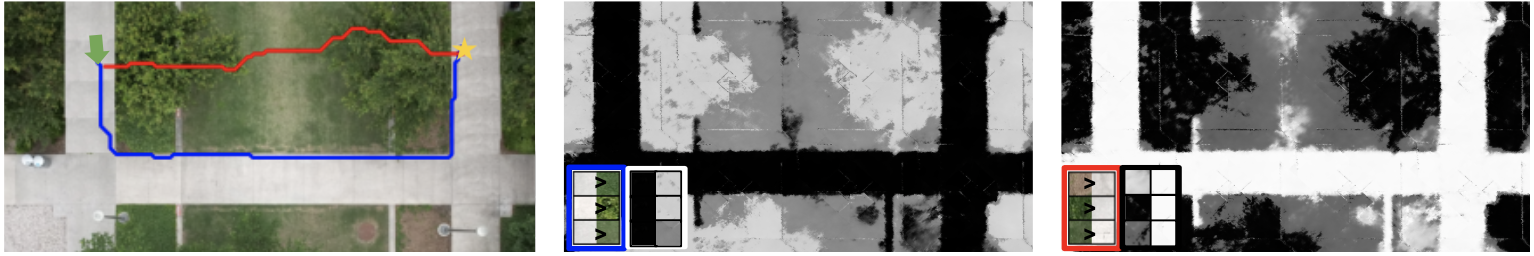
Figure 4: The effect of changing preference on path planning is shown on the left image of an aerial map. The blue path corresponds to the middle costmap and the red path corresponds to the right costmap. The generated costmaps reflect the preferences provided in the context. Black corresponds to low cost and white corresponds to high cost.

VI-A Aerial Map Experiments

In our simulated experiments, we build aerial maps from drone footage of three locations around our campus, which we consider seen environments. We also use open-source aerial maps [23] from around the world, covering a wide variety of both urban and natural terrain types and which we consider unseen. For each of the seen and unseen environments, we provide a start and goal location and test varying operator preferences. We test realistic preferences, and “inverted” preferences, in which each of the pairwise orderings in the realistic preference are reversed. Given the robot’s pose on the aerial map, the robot’s projected bird’s eye view can be found, and used as input to generate the local costmap. Planning is done using the A* algorithm [24] on the costmap.

Table II displays the results for seen environments. Towards answering question 1a, pacer has similar results to the sterling baseline, as both approaches were trained on the same in-distribution data. When no useful context has been provided for pacer (i.e. the context contains only unseen terrains which do not match the environment as per 1b), the results are on par with the classifier baseline. pacer’s success despite the lack of an informative preference context shows that the model has captured a prior over realistic cost-assignment for in-distribution terrains.

Table II displays the results for unseen environments. Towards answering question 2a, when given an informative context, pacer outperforms the sterling baseline. Though representation-learning approaches like sterling should theoretically generalize due to their continuous representation space, this is contingent on similar terrains forming clusters in this space, which may not be the case for unseen terrains. Note that here, for unseen environments, the classifier baseline has been omitted, as it allows no way for a user to provide terrain preferences for classes that are not predefined. pacer overcomes the limitations of previous paradigms, as it both allows preferences in unseen environments to be expressed and generalizes well to these unseen environments. Additionally, when no useful context has been provided for the unseen terrains (per 2b), pacer is not able to adapt.

Method	Low (%)	Medium (%)	High (%)
pacer	73.83%	19.70%	6.47%
pacer (uninformative context)	67.97%	15.89%	16.15%
sterling	74.72%	18.65%	6.63%
Classifier	65.86%	21.46%	12.69%
Upper Bound	82.82%	13.69%	3.49%

TABLE I: Proportion of planned paths that traverse low, medium, and high-cost terrains in seen environments, relating to 1a,1b.

Method	Low (%)	Medium (%)	High (%)
pacer	81.85%	8.00%	10.15%
pacer (uninformative context)	53.83%	2.20%	43.97%
sterling	61.39%	10.12%	26.86%
Upper Bound	91.85%	6.02%	2.13%

TABLE II: Proportion of planned paths that traverse low, medium, and high-cost terrains in unseen environments, relating to 2a,2b.

	Low (%)	Medium (%)	High (%)
Realistic Preference
$\mathcal{D}_{\mathrm{real}}$	95.97%	1.70%	2.32%
$\mathcal{D}_{\mathrm{shuffled}}$	70.50%	18.94%	10.55%
$\mathcal{D}_{\mathrm{synthetic}}$	76.66%	18.43%	4.91%
Inverted Preference
$\mathcal{D}_{\mathrm{real}}$	18.55%	20.97%	60.48%
$\mathcal{D}_{\mathrm{shuffled}}$	69.21%	22.56%	8.23%
$\mathcal{D}_{\mathrm{synthetic}}$	70.22%	21.32%	8.46%
Uninformative Context
$\mathcal{D}_{\mathrm{real}}$	66.22%	14.48%	19.30%
$\mathcal{D}_{\mathrm{shuffled}}$	81.82%	7.67%	10.51%
$\mathcal{D}_{\mathrm{synthetic}}$	67.97%	15.89%	16.15%

TABLE III: Proportion of planned paths that traverse low, medium, and high-cost terrains in seen environments for each training phase. The model after each phase of training is tested using realistic, inverted, and uninformative contexts

Method	Low (%)	Medium (%)	High (%)
Realistic Preference
$\mathcal{D}_{\mathrm{real}}$	60.78%	7.05%	32.18%
$\mathcal{D}_{\mathrm{shuffled}}$	65.16%	6.44%	28.40%
$\mathcal{D}_{\mathrm{synthetic}}$	88.09%	2.57%	9.34%
Inverted Preference
$\mathcal{D}_{\mathrm{real}}$	22.59%	15.31%	62.10%
$\mathcal{D}_{\mathrm{shuffled}}$	39.86%	13.96%	46.17%
$\mathcal{D}_{\mathrm{synthetic}}$	65.65%	22.10%	12.25%
No Context
$\mathcal{D}_{\mathrm{real}}$	73.44%	7.50%	19.06%
$\mathcal{D}_{\mathrm{shuffled}}$	82.35%	4.65%	13.00%
$\mathcal{D}_{\mathrm{synthetic}}$	53.83%	2.20%	43.97%

TABLE IV: Proportion of planned paths that traverse low, medium, and high-cost terrains in unseen environments for each training phase. The model after each phase of training is tested using realistic, inverted, and uninformative contexts

VI-B Ablation Study

To understand the effects of each phase in the training process, we perform an ablation study using the same environments as in the aerial simulator experiments.

In the $\mathcal{D}_{\mathrm{real}}$ phase, the model is trained only on real data and realistic preferences. In the $\mathcal{D}_{\mathrm{shuffled}}$ phase, the model is pretrained on real data with realistic preferences, and then trained on a smaller amount of changed preferences. In $\mathcal{D}_{\mathrm{synthetic}}$ phase, the model is trained according to all three phases.

Results are shown in Tab. IV, IV. In seen environments, the model trained on $\mathcal{D}_{\mathrm{real}}$ performs the best of the three with realistic preferences, but is unable to adapt when the preferences are inverted. Even without a useful context provided, the majority of planned trajectories are on low-cost terrain. In unseen environments, this method performs the worst regardless of preference context. The model trained on $\mathcal{D}_{\mathrm{shuffled}}$ is able to adapt to changing preference orderings in seen environments, though is unable to recognize and match new terrains in the preference context to the new environment. The model trained on $\mathcal{D}_{\mathrm{synthetic}}$ is shown to both respect changing preference order and recognize new terrains.

VI-C Discussion

The results presented in this section demonstrate that pacer fulfills our three design desiderata. The adherence of pacer to realistic preferences when not given an informative preference context fulfills the first key property of being able to make inferences when there is no context by capturing a prior over realistic preferences (1b). As per the second key property, pacer has been shown to align costs to preferred terrains even as preferences are varied (1a). An example of paths planned according to different preferences is shown in Fig. 4. The performance of pacer in both seen and unseen environments when given an informative preference context shows that pacer exhibits the third key property (1a, 2a).

VII Real Robot Experiments

We now seek to demonstrate that pacer performs well during execution in the real world. We deploy our method, sterling, and the classifier approach on a mobile robot at four different locations on the UT campus which are not included in the simulated environments. These four locations cover red brick, concrete sidewalk, grass, mulch, and pebble pavement.

Since all methods are trained to be view-point invariant and platform-agnostic, we trained them all with the same data collected from a Boston Dynamics Spot, and deployed zero-shot on a Clearpath Jackal which has significant differences in viewpoint and mobility than the Spot. We evaluate the performance of each method with a realistic preference on a variety of terrain types. In these experiments, we measure the robot’s ability to execute the plan, which includes robustness to a different viewpoint and platform. We integrate each method with a sampling-based local planner [25] and maintain the same planner parameters to ensure fairness.

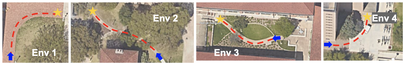
Figure 5: The four environments where real-robot trials were performed. Blue arrows and yellow stars show start and goal locations respectively. The red dashed line marks the intended path based on operator preference.

Environment	Env 1	Env 2	Env 3	Env 4
Classifier	5/5	4/5	1/5	2/5
sterling	0/5	2/5	0/5	4/5
Ours	5/5	5/5	5/5	4/5

TABLE V: Number of successes per 5 trials of different approaches across various environments. A trial is a success if the robot reaches the goal without traversing across undesirable terrain and without operator intervention.

Table V shows results from real robot experiments. Our approach had the most successful trials across all environments. While the classifier performed well in environments 1 and 2, we hypothesize that difficult lightning conditions and variations in terrain appearance caused the failures in environments 3 and 4. Though sterling performed as the best baseline in the simulated experiments (which involved only planning), it seemed to be unable to execute these plans in real-robot experiments. Many of the failure cases involved the robot driving slightly off-path and just grazing the undesirable terrains. In patch-based representations, a single patch may contain multiple different terrains (e.g. half sidewalk and half grass), so the cost assigned to the patch would be some combination of the different terrain costs, resulting in a coarser degree of control on the physical robot. Our approach overcomes this limitation since it directly outputs a fine-grained costmap in a single forward pass.

VIII Limitations and Future Work

The experiments reported in this paper were conducted on a single campus with one robot. Future work should extend the study to more varied terrains and deploy multiple robots with diverse sensors. Additionally, we aim to evaluate the ease with which human users can express preferences using our method, as well as explore alternative mechanisms for preference expression in costmap generation. Incorporating depth data into the costmap generation is another key area for improvement, as our current reliance on a homography transformation assumes flat ground, leading to limitations like the inability to avoid obstacles such as concrete curbs, despite their preferable terrain.

IX Conclusion

In this paper we presented pacer, a novel architecture and training approach to quickly produce costmaps according to arbitrary user preferences and new terrains with no fine-tuning. Our approach was evaluated against semanics-based and representation-learning baselines in both simulated and real robot experiments. We have shown this approach to be highly adaptable to new preferences and terrains, as well as able to infer the traversability of some terrains according to realistic preferences.

X Acknowledgements

This work has taken place in the Autonomous Mobile Robotics Laboratory (AMRL) at UT Austin. AMRL research is supported in part by NSF (CAREER-2046955, OIA-2219236, DGE-2125858, CCF-2319471), ARO (W911NF-23-2-0004), Amazon, and JP Morgan. Any opinions, findings, and conclusions expressed in this material are those of the authors and do not necessarily reflect the views of the sponsors.

A portion of this work has taken place in the Learning Agents Research Group (LARG) at UT Austin. LARG research is supported in part by NSF (FAIN-2019844, NRT-2125858), ONR (N00014-18-2243), ARO (W911NF-23-2-0004, W911NF-17-2-0181), Lockheed Martin, and UT Austin’s Good Systems grand challenge. Peter Stone serves as the Executive Director of Sony AI America and receives financial compensation for this work. The terms of this arrangement have been reviewed and approved by the University of Texas at Austin in accordance with its policy on objectivity in research.

Hyperparameter	Value
Learning Rate (lr)	1e-5
Batch Size	64
Number of Epochs (Phase 1)	100
Number of Epochs (Phase 2)	5
Number of Epochs (Phase 3)	100
Optimizer	Adam
Activation Function	Sigmoid
Kernel	3
Stride	1

TABLE VI: Model-training hyperparameters.

Terrain Type	Number of Patches
Bush	612
Concrete	846
Marble rock	748
Mulch	838
Pebble pavement	879
Grass	878

TABLE VII: Number of patches for each terrain type

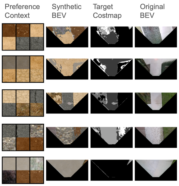
Figure 6: Synthetic data examples consisting of Preference Context, Synthetic BEV, and Target Costmap, generated by segmenting and replacing terrains from the Original BEV.

Appendix A Dataset Details

In this section, we provide the size and statistics of our dataset. We train with four “realistic” preferences, each with a plausible reason for the ordering. Legged robots may encounter resistance on bush, but would trip on marble rock so fitting operator preferences are: (1) $\texttt{pebble}\succ\texttt{concrete}\succ\texttt{mulch}\succ\texttt{grass}\succ\texttt{bush}\succ\texttt{marble}$ or (2) $\texttt{concrete}\succ\texttt{pebble}\succ\texttt{grass}\succ\texttt{mulch}\succ\texttt{bush}\succ\texttt{marble}$. On the other hand, wheeled robots will slip a bit on marble rock, but cannot drive through bush so a realistic preference is: (3) $\texttt{concrete}\succ\texttt{pebble}\succ\texttt{mulch}\succ\texttt{grass}\succ\texttt{marble}\succ\texttt{bush}$. As an example of a preference motivated by social norms, we have: (4) $\texttt{concrete}\succ\texttt{pebble }\succ\texttt{marble}\succ\texttt{grass}\succ\texttt{bush}\succ\texttt{mulch}$ since it is undesirable for robots to trample grass lawns, but doing so to marble rock is alright.

To construct a large training dataset from a relatively small amount of recorded data, we employ synthetic augmentation using 14 additional terrain textures, including sand, asphalt, leaves, river pebbles, cracked mud, and snow. Examples of synthetically augmented data are shown in Fig 6. Model training hyperparameters and statistics for the patch bank are shown in Tab. VII and Tab. VII.

Appendix B Aerial Map Simulator

In Fig 7 and 8, we show examples of paths planned using pacer in our aerial map simulator. These experiments are an evaluation purely over planning based on terrain preference, with no kinodynamic constraints, no errors due to localization, and no costs associated with elevation.

Given a robot state $(x,y,\theta)$ relative to the map, the robot’s view from this pose is found by overlaying the warped field-of-view shape onto the aerial map at that state. We employ A* on an eight-connected grid for path planning on the local costmap. If the node-expansion operation in A* explores a neighbor node which does not have an associated cost (meaning its state has not been captured in any previous view), the BEV from the current node is used to construct a local costmap which includes the previously-unobserved neighbor state, and the planning continues. Thus, the robot does not actually move its position in this path planning simulation. This is an optimization such that we can avoid transforming the full aerial map (which may be very large) into a costmap. Fig 7 shows the progression of the local costmaps as the robot discovers more of the environment and the resulting planned path.

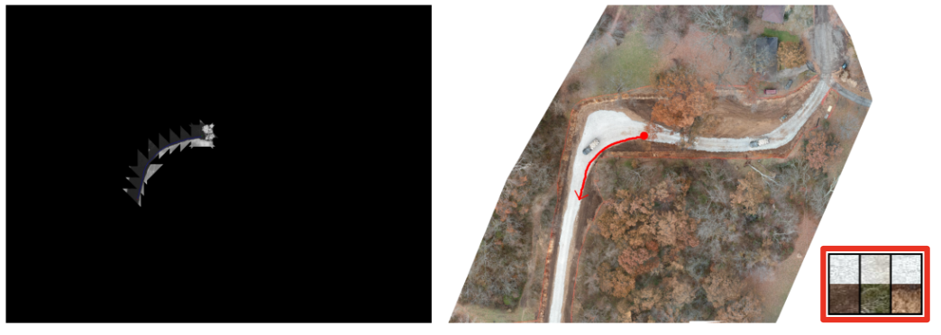
Figure 7: Example of a costmap, planned path, and preference context of a simulated robot deployment in one of the natural unseen environments of the Aerial Map Experiments using our method. The costmap displays the timeseries progression of the local BEV costmaps generated with our method.

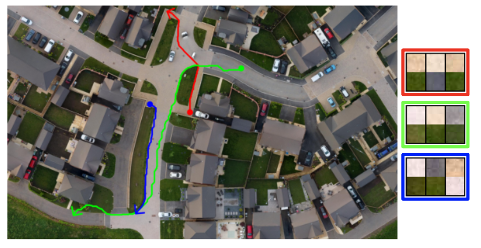
Figure 8: Examples of several paths planned using our method in an urban unseen environment and their corresponding preference contexts. Here, we visualize the large scale of these simulated deployments, and the diversity of visual terrain appearances.

Appendix C Real Robot Experiments Setup

We run our real-robot experiments on a Clearpath Jackal Unmanned Ground Vehicle. A Microsoft Azure Kinect RGB-D camera supplies visual information at $\sim\!30\text{Hz}$. We run all algorithms on a Nvidia GeForce GTX 1050Ti GPU. Taking advantage of batched cost computation on the GPU, we find that the sterling and classifier baselines publish motion commands at $\sim\!20\text{Hz}$. Our approach publishes motion commands at $\sim\!11\text{Hz}$ on the same GPU since our approach outputs full costmaps, which is done sequentially.

Though each method was trained using data collected from a Boston Dynamics Spot, they were all deployed zero-shot on the Clearpath Jackal with only visual input. While most experimental results reported in sterling were obtained using a joint representation space with both visual and inertial-propriceptive-tactile features deployed on the legged Spot, the approach claims to be broadly adaptable to robots of different morphology with vision-only navigation. We follow the precedent set in sterling of transferring visual features learned from the Spot to the Jackal.

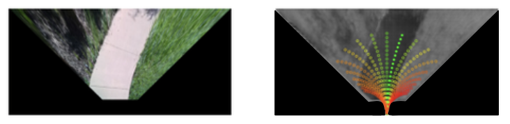
Figure 9: Example of homography-transformed BEV image of live robot deployment and corresponding local costmap. The best local plan is chosen from a set of path options based on a weighted combination of the terrain cost and distance to goal.

C-A Sampling-based Preference-aligned Local Planning Formulation

We formalize the local path planning problem as a search for the optimal motion arc $\Gamma^{*}$ from a set of arc options $\{\Gamma_{1},\Gamma_{2},\ldots,\Gamma_{n}\}$, each of which adheres to the kinodynamic constraints of Ackermann Steering (Fig 9). Each arc $\Gamma_{i}$ represents a feasible trajectory that the robot can follow, and is discretized into states/actions at finite future timestamps in a receding horizon planner. Each arc can be expressed as $\Gamma_{i}=\{s_{0},s_{1},\ldots,s_{m}\}$, where $s_{0}$ is the current state and $s_{m}$ is the state at the end of the planning horizon. More precisely, given a cost function $\mathcal{J}$, the optimal arc $\Gamma^{*}$ is

$$\Gamma^{*}=\arg\min_{\Gamma}\mathcal{J}(\Gamma,G)\;,$$

where

$$\mathcal{J}(\Gamma_{i},G)=\alpha\cdot\mathcal{J}_{\text{geometric}}(\Gamma_{i},G)+(1-\alpha)\cdot\mathcal{J}_{\text{terrain}}(\Gamma_{i})\;,$$

and $\alpha$ is the parameter representing the tradeoff between the geometric and terrain costs in the arc selection. $\mathcal{J}_{\text{geometric}}(\Gamma_{i},G)$ measures the geometric distance between the goal $G$ and the closest state in $\Gamma_{i}$. $\mathcal{J}_{\text{terrain}}(\Gamma_{i},G)$ is the terrain-cost of $\Gamma_{i}\in\{\Gamma_{1},\Gamma_{2},\ldots,\Gamma_{n}\}$, formulated as follows:

$$\mathcal{J}_{\text{terrain}}(\Gamma_{i})=\sum_{s_{j}\in\Gamma_{i}}\gamma^{j}\cdot C(s_{j})\;,$$

where the term $\gamma^{j}$ represents a decay factor applied to the cost of each state $s_{j}$ along the arc $\Gamma_{i}$ such that the planner prioritizes short-term navigational feasibility. In our experiments, we use $\gamma=0.9$. The cost at state $s_{j}$, $C(s_{j})$, is calcuated either by indexing into the full BEV costmap (as with pacer) or via terrain patch to scalar cost (as with the sterling and classifier baselines).

Having determined $\Gamma^{*}$, a finite action control sequence is obtained by applying 1D time optimal control along $\Gamma^{*}$, resulting in a series of control inputs that drive the robot along the optimal path.

Appendix D Preference Context Embeddings

We include a t-SNE visualization of the embedding space of the context encoder in Fig. 10. We display only the realistic preference contexts (red) and inverted preference contexts (blue), as the differences in other variations of preference context are much more subtle. The separation between realistic preference contexts (red) and inverted preference contexts (blue) indicate the encoder has learned useful features on which condition the output costmap.

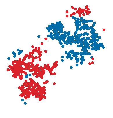
Figure 10: Visualization of t-SNE plot showing embedding vectors of realistic preference contexts (red) and inverted preference contexts (blue).

References

- [1] X. Xiao, Z. Xu, Z. Wang, Y. Song, G. Warnell, P. Stone, T. Zhang, S. Ravi, G. Wang, H. Karnan, J. Biswas, N. Mohammad, L. Bramblett, R. Peddi, N. Bezzo, Z. Xie, and P. Dames, “Autonomous ground navigation in highly constrained spaces: Lessons learned from the barn challenge at icra 2022,” 2022.
- [2] X. Xiao, Z. Xu, G. Warnell, P. Stone, F. G. Guinjoan, R. T. Rodrigues, H. Bruyninckx, H. Mandala, G. Christmann, J. L. Blanco-Claraco, and S. S. Rai, “Autonomous ground navigation in highly constrained spaces: Lessons learned from the 2nd barn challenge at icra 2023,” 2023.
- [3] X. Xiao, B. Liu, G. Warnell, and P. Stone, “Motion planning and control for mobile robot navigation using machine learning: a survey,” 2022.
- [4] H. Karnan, A. Nair, X. Xiao, G. Warnell, S. Pirk, A. Toshev, J. Hart, J. Biswas, and P. Stone, “Socially compliant navigation dataset (scand): A large-scale dataset of demonstrations for social navigation,” 2022.
- [5] X. Meng, N. Hatch, A. Lambert, A. Li, N. Wagener, M. Schmittle, J. Lee, W. Yuan, Z. Chen, S. Deng, G. Okopal, D. Fox, B. Boots, and A. Shaban, “Terrainnet: Visual modeling of complex terrain for high-speed, off-road navigation,” 2023.
- [6] M. Wigness, J. G. Rogers, and L. E. Navarro-Serment, “Robot navigation from human demonstration: Learning control behaviors,” in 2018 IEEE International Conference on Robotics and Automation (ICRA), 2018, pp. 1150–1157.
- [7] M. Wulfmeier, D. Rao, and I. Posner, “Incorporating human domain knowledge into large scale cost function learning,” 2016.
- [8] G. Kahn, P. Abbeel, and S. Levine, “Badgr: An autonomous self-supervised learning-based navigation system,” 2020.
- [9] ——, “Land: Learning to navigate from disengagements,” CoRR, vol. abs/2010.04689, 2020. [Online]. Available: https://arxiv.org/abs/2010.04689
- [10] A. H. Raj, Z. Hu, H. Karnan, R. Chandra, A. Payandeh, L. Mao, P. Stone, J. Biswas, and X. Xiao, “Rethinking social robot navigation: Leveraging the best of two worlds,” 2024.
- [11] D. Fox, W. Burgard, and S. Thrun, “The dynamic window approach to collision avoidance,” IEEE Robotics & Automation Magazine, vol. 4, no. 1, pp. 23–33, 1997.
- [12] G. Williams, P. Drews, B. Goldfain, J. M. Rehg, and E. A. Theodorou, “Aggressive driving with model predictive path integral control,” in 2016 IEEE International Conference on Robotics and Automation (ICRA), 2016, pp. 1433–1440.
- [13] S. Macenski, T. Moore, D. V. Lu, A. Merzlyakov, and M. Ferguson, “From the desks of ros maintainers: A survey of modern &; capable mobile robotics algorithms in the robot operating system 2,” Robotics and Autonomous Systems, vol. 168, p. 104493, Oct. 2023. [Online]. Available: http://dx.doi.org/10.1016/j.robot.2023.104493
- [14] H. Karnan, E. Yang, D. Farkash, G. Warnell, J. Biswas, and P. Stone, “Sterling: Self-supervised terrain representation learning from unconstrained robot experience,” 2023.
- [15] K. S. Sikand, S. Rabiee, A. Uccello, X. Xiao, G. Warnell, and J. Biswas, “Visual representation learning for preference-aware path planning,” CoRR, vol. abs/2109.08968, 2021. [Online]. Available: https://arxiv.org/abs/2109.08968
- [16] H. Karnan, E. Yang, G. Warnell, J. Biswas, and P. Stone, “Wait, that feels familiar: Learning to extrapolate human preferences for preference aligned path planning,” 2023.
- [17] P. Jiang, P. R. Osteen, M. B. Wigness, and S. Saripalli, “RELLIS-3D dataset: Data, benchmarks and analysis,” CoRR, vol. abs/2011.12954, 2020. [Online]. Available: https://arxiv.org/abs/2011.12954
- [18] T. Guan, D. Kothandaraman, R. Chandra, and D. Manocha, “Ganav: Group-wise attention network for classifying navigable regions in unstructured outdoor environments,” CoRR, vol. abs/2103.04233, 2021. [Online]. Available: https://arxiv.org/abs/2103.04233
- [19] X. Yao, J. Zhang, and J. Oh, “Rca: Ride comfort-aware visual navigation via self-supervised learning,” 2022. [Online]. Available: https://arxiv.org/abs/2207.14460
- [20] J. Zürn, W. Burgard, and A. Valada, “Self-supervised visual terrain classification from unsupervised acoustic feature learning,” 2019. [Online]. Available: https://arxiv.org/abs/1912.03227
- [21] T. Miki, L. Wellhausen, R. Grandia, F. Jenelten, T. Homberger, and M. Hutter, “Elevation mapping for locomotion and navigation using gpu,” 2022. [Online]. Available: https://arxiv.org/abs/2204.12876
- [22] P. Haven, “Poly haven textures,” 2024, accessed: 2024-06-05. [Online]. Available: https://polyhaven.com/textures
- [23] O. Contributors, “Openaerialmap: An open source platform for aerial imagery,” 2024, accessed: 2024-06-05. [Online]. Available: https://www.openaerialmap.org/
- [24] P. Hart, N. Nilsson, and B. Raphael, “A formal basis for the heuristic determination of minimum cost paths,” IEEE Transactions on Systems Science and Cybernetics, vol. 4, no. 2, pp. 100–107, 1968. [Online]. Available: https://doi.org/10.1109/tssc.1968.300136
- [25] J. Biswas, “Amrl autonomy stack,” 2013, accessed: 2024-06-05. [Online]. Available: https://github.com/ut-amrl/graph_navigation