A graph-based algorithm for the non-stationary lot-sizing problem with penalty scheme

Abstract

This paper introduces a graph-based algorithm for solving single-item, single-location inventory lot-sizing problems under non-stationary stochastic demand using the $(R_{t},S_{t})$ policy and a penalty cost scheme. The proposed method relaxes the original mixed-integer linear programming (MILP) model by eliminating non-negative order quantity constraints and formulating it as a shortest-path problem on a weighted directed acyclic graph. A repetitive augmentation procedure is proposed to resolve any infeasibility in the solution. This procedure consists of three stages: (1) filtration, (2) repeated augmentation by redirecting, reconnecting, and duplicating between newly introduced and existing nodes to adjust the graph and eliminate negative replenishment orders, and (3) re-optimising. The effectiveness and computational efficiency of the proposed approach are assessed through extensive experiments on 1,620 test instances across various demand patterns and parameter settings. The results show that 195 instances required augmentation, mainly those with high penalty costs, low fixed ordering costs, large demand variability, and extended planning horizons. The efficiency of the algorithm for instances with extended planning horizon scenarios demonstrates its suitability for use in real-world scenarios.

Keywords inventory control, lot-sizing problem, non-stationary demand, uncertainty strategy, shortest path problem.

1 Introduction

The study of lot-sizing problems starts with Harris, (1913) and expands to incorporate more realistic assumptions on customer demand. Wemmerlöv, (1989) illustrates that lot-sizing studies need to be undertaken in stochastic dynamic environments with at least a modicum of resemblance to reality, for which a class of research considers non-stationary stochastic demand.

To address demand uncertainty, Bookbinder and Tan, (1988) propose three uncertainty strategies and develop a heuristic for the static-dynamic strategy. This strategy statically determines one parameter (either order quantity or order timing) at the start of the planning horizon and dynamically determines the other in a wait-and-see manner. This uncertainty strategy is further adapted into ($R_{t},S_{t}$) and ($s_{t},Q_{t}$) policies for non-stationary stochastic demand. The ($R_{t},S_{t}$) policy applies fixed reorder timings $R_{t}$, at which the replenishment quantity is dynamically determined by setting the order-up-to level $S_{t}$ in advance, while the actual order quantity is decided only when the order is issued. An alternative to the $(R_{t},S_{t})$ policy is the ($s_{t},Q_{t}$) policy, where for each period $t$, an order with quantity $Q_{t}$ is issued when inventory falls below or at the reorder threshold $s_{t}$ (reorder point). While Scarf, (1960) shows that the optimal policy for dynamic inventory issues is an ($s_{t},S_{t}$) policy under convex holding and penalty costs, practical challenges arise in supply chains where clients frequently change order schedules and volumes. Developing models that can pre-plan order timings for stochastic demand is crucial for enhancing cooperation and coordination.

Therefore, in the context of non-stationary stochastic demand and focusing on the $(R_{t},S_{t})$ policy, Tarim and Kingsman, (2004) present a mixed-integer programming formulation to determine the order schedule and order-up-to levels of the $(R_{t},S_{t})$ policy under non-stationary settings, simultaneously in a single step, for the $\alpha$ service level problem. This formulation is adapted by Tempelmeier, (2007) for the $\alpha_{c}$ service level, and by Rossi et al., (2015) for the $\beta$ and $\beta^{cyc}$ service levels, as well as for the penalty cost scheme with back-orders. Apart from modelling service levels, Tarim and Kingsman, (2006) provide another MIP formulation to account for shortage costs, where the objective function is obtained using a piecewise linear approximation. The accuracy of the approximation can be adjusted by introducing new breakpoints. This piecewise linear approximation is detailed in Rossi et al., (2014), with segmentation parameters provided for the Normal distribution.

In the literature, mathematical formulations or heuristics for the $(R_{t},S_{t})$ policy tend to focus more on service levels (particularly the $\alpha$ service level) than on penalty costs. In service-level settings, inventory is maintained at a level that meets a target non-stockout probability; this limits shortages and simplifies cost control by focusing on fulfilment rather than shortage costs. In contrast, penalty schemes explicitly incorporate the costs of unmet demand into the expected total cost through either back-orders or lost sales, without setting a predefined inventory boundary; this adds complexity to the model.

Tarim and Kingsman,’s model of the $(R_{t},S_{t})$ policy is reformulated by Tunc et al., (2014) by decoupling consecutive replenishment periods, based on a MIP formulation using the network flow structure of the problem. This formulation has a tighter linear relaxation and, in turn, superior computational performance. Tunc et al., (2018) generalise this model and develop a dynamic cut generation approach combined with the piecewise linear approximation by Rossi et al., (2015), which enjoys the computational efficiency from the reformulation of Tunc et al., (2014) and the modelling flexibility of Rossi et al., (2015). Özen et al., (2012) consider both penalty cost and service level and prove that the optimal policy under the static-dynamic uncertainty strategy is the base stock policy for both penalty and service-level constrained models with capacity limitations and minimum order quantity requirements.

The aforementioned formulations operate under the assumption that a negative order is not allowed; in other words, retailers cannot sell back excess stock to the warehouse and must carry the stock forward to the next period. Tarim et al., (2011) relax this constraint and propose a computationally efficient MILP relaxation that provides an optimal solution. They also show that an infeasible solution yields a tight lower bound for the optimal cost and that this infeasible solution can be easily modified to obtain a feasible solution, which provides an upper bound. In the algorithm developed by Tarim et al., (2011), an optimal solution is obtained by iteratively solving a relaxed version of the problem that is formulated and solved as a shortest-path problem. In case of infeasibility, the relaxation approach is applied at each node of the search tree within a branch-and-bound procedure to efficiently search for an optimal solution. Through a filtering and augmenting procedure, Rossi et al., (2011) refine this approach. Starting from a relaxed state space graph, the method proposed by Rossi et al., (2011) eliminates provably sub-optimal arcs and states (filtering), and then efficiently constructs (augmenting) a reduced state space graph representing the original problem.

This study focuses on the single-item single-location non-stationary stochastic lot-sizing problem under a penalty cost scheme, with unmet demand considered as back-orders. We develop an algorithm to efficiently approximate the optimal $(R_{t},S_{t})$ policy parameters.

Our research contributes to the literature in three aspects as follows.

• We develop an efficient graph-based approach to determine the $(R_{t},S_{t})$ policy parameters in a non-stationary stochastic lot-sizing problem. In contrast to the service-level-based formulations commonly addressed in existing literature, our method operates under a penalty cost scheme with backordered unmet demand.

• We transform the original $(R_{t},S_{t})$ MILP model into a weighted directed acyclic graph through a relaxation that captures the expected cycle costs. To resolve the infeasibility introduced by negative replenishment orders, we develop a repetitive augmentation procedure. This procedure iteratively refines the solution until the negative replenishment orders are eliminated from the graph, ensuring the feasibility of the final solution.

• We validate the efficiency, reliability, and scalability of the proposed graph-based approach through comprehensive computational experiments. Solutions without negative replenishment orders consistently achieve the exact optimal cost. In cases where infeasibilities occur, the repetitive augmentation procedure effectively resolves them, optimising the policy parameters while maintaining minimal deviation from the relaxed problem.

The remainder of the paper is organised as follows: Section 2 defines the problem and presents a mixed integer linear programming model for the $(R_{t},S_{t})$ policy. Section 3 introduces a relaxation of the original problem by removing the negative order quantity constraint and deriving an equivalent shortest-path formulation using a weighted directed acyclic graph. Section 4 proposes the repetitive augmenting algorithm to resolve infeasibilities in the relaxed solution. Section 5 provides an illustrative example to demonstrate the development from the optimal policy to the proposed graph-based approach for the ($R_{t},S_{t}$) policy. Section 6 evaluates the computational efficiency and effectiveness of the proposed method through comprehensive numerical experiments. Notation applied in this work are listed in the Appendix A.

2 Problem description and preliminary formulations

In a single-item single-location non-stationary stochastic lot-sizing problem over a planning horizon of $T$ periods, replenishment orders are placed and delivered instantaneously at the start of each period. The demands $d_{t}$, for $t=1,\dots,T$, are independent random variables with known probability density functions $\varphi_{t}(\cdot)$. Each time an order is placed, an ordering cost $c(Q_{t})$ is incurred, comprising a fixed ordering cost $K$ and a linear ordering cost $z$ proportional to the non-negative order quantity $Q_{t}$ in period $t$. Specifically, the ordering cost is $c(Q_{t})=K+zQ_{t}$ when an order is placed, where $Q_{t}\geq 0$. Placing an order of zero quantity ($Q_{t}=0$) is allowed and still incurs the fixed ordering cost $K$. If no order is placed in period $t$, then no ordering cost is incurred. Placing an order with zero quantity allows the system to update the order status and inventory levels without changing the actual stock on hand. This action can be optimal to reduce nervousness (De Kok and Inderfurth,, 1997; Rossi et al.,, 2011) and to better design the replenishment cycle.

After satisfying demand, at the end of each period, a linear holding cost $h$ is incurred for each unit carried from one period to the next, and a linear penalty cost $b$ is charged on each unit back-ordered. Then the expected immediate cost at the end of period $t$ can be expressed as

$$L_{t}(y)=h\mathbb{E}[\max(y-d_{t},0)]+b\mathbb{E}[\max(d_{t}-y,0)],$$ (1)

where $y$ denotes the inventory level after receiving the replenishment and $\mathbb{E}$ denotes taking the expectation. Let the notation $\tilde{\cdot}$ denote the expectation of a random variable. For period $t$, we let $\tilde{H}_{t}(y)=\mathbb{E}[\max(y-d_{t},0)]$ denote the expected inventory carried from period $t$ to period $t+1$, $\tilde{B}_{t}(y)=\mathbb{E}[\max(d_{t}-y,0)]$ denote the expected back-ordered level, and $\tilde{I}_{t}(y)$ denote the expected closing inventory at the end of period $t$, where

$$\tilde{I}_{t}(y)=\tilde{H}_{t}(y)-\tilde{B}_{t}(y).$$ (2)

Then Eq.(1) can be re-written as

$$L_{t}(y)=h\tilde{H}_{t}(y)+b\tilde{B}_{t}(y).$$ (3)

Let $C_{t}(x)$ be the expected total cost of an optimal policy over periods $t$ to $T$ with the opening inventory level $x$, then the problem can be modelled as a stochastic dynamic program (Bellman,, 1957) as

$$C_{t}(x)=\min_{y\geq x}\{c(y-x)+L_{t}(y)+\mathbb{E}[C_{t+1}(y-d_{t})]\},$$ (4)

where $C_{T+1}(x)=0$ is the boundary condition. We remark that the optimisation works on the constraint $y\geq x$, representing a non-negative replenishment.

Rossi et al., (2015) apply the $(R_{t},S_{t})$ policy and introduce a MILP to approximate the expected total cost for a single-item single-location inventory system with non-stationary stochastic demand. In this paper, we modify their model by replacing the expected order-up-to level $\tilde{S}_{t}$ with the expected order quantity $\tilde{Q}_{t}$, which will facilitate further adaptations in subsequent sections.

$$\min\quad \displaystyle\sum_{k=t}^{T}(\delta_{k}K+z\tilde{Q}_{k}+h\tilde{H}_{k}+b\tilde{B}_{k}),$$ (5)

s.t. $$\delta_{k}=0\rightarrow\tilde{I}_{k}+\tilde{d}_{k}-\tilde{I}_{k-1}=0, k=t,\ldots,T,$$ (6)

$$\delta_{k}=1\rightarrow\tilde{I}_{k}+\tilde{d}_{k}-\tilde{I}_{k-1}=\tilde{Q}_{k}, k=t,\ldots,T,$$ (7)

$$P_{j,k}\geq\delta_{j}-\sum\limits_{r=j+1}^{k}\delta_{r}, k=t,\ldots,T,\mathop{}j=t,\ldots,k,$$ (8)

$$\sum\nolimits_{j=t}^{k}P_{j,k}=1, k=t,\ldots,T,$$ (9)

$$P_{j,k}=1\rightarrow\tilde{H}_{k}=\hat{\mathcal{L}}(\tilde{I}_{k}+\tilde{d}_{j,k},d_{j,k}), k=t,\ldots,T,\mathop{}j=t,\ldots,k,$$ (10)

$$P_{j,k}=1\rightarrow\tilde{B}_{k}=\mathcal{L}(\tilde{I}_{k}+\tilde{d}_{j,k},d_{j,k}), k=t,\ldots,T,\mathop{}j=t,\ldots,k,$$ (11)

$$\tilde{H}_{k},\tilde{B}_{k}\geq 0,\quad P_{j,k},\delta_{k}\in\{0,1\}, k=t,\ldots,T,\mathop{}j=t,\ldots,k.$$ (12)

The objective function denotes the expected total cost over horizon $(t,T)$. Constraints (6) and (7) apply the indicator constraints (Belotti et al.,, 2016) to demonstrate the inventory flow balance, where $\delta_{k}$ is a binary variable denoting the order decision in period $k$. This model introduces a binary variable $P_{j,k}$ to properly account for demand variance while computing the first-order loss function. Let $P_{j,k}$ ($j\leq k$) take the value of 1 if the last order before period $k$ (including period $k$ itself) is placed at the beginning of period $j$. Note that the combination of constraints (8) and (9) ensures that demand variance is properly accounted for even when no order takes place within the horizon ($j,k$).

For the convenience of notation, this paper defines the replenishment cycle $R(i,j)$ as periods $i,i+1,\ldots,j$ covered by one replenishment order placed at period $i$, where $\delta_{i}=1$, $\delta_{i+1},\ldots,\delta_{j}=0$, and $\delta_{j+1}=1$, as illustrated in Figure 1. For any period in the replenishment cycle $R(j,k)$ ($j\leq k$), the expected closing inventory level is modelled by constraints (10) and (11) by means of the first order loss function $\mathcal{L}$ and its complementary $\hat{\mathcal{L}}$, where $\tilde{I}_{k}+\tilde{d}_{j,k}$ is the opening inventory of replenishment cycle $R(j,k)$ and $d_{j,k}$ is the cumulative demand over the horizon ($j,k$).

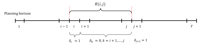
Figure 1: A replenishment cycle $R(i,j)$ over period $i$ to $j$.

3 A shortest-path formulation of ($\bm{R_{t},S_{t}}$) policy

This section introduces a relaxation of the $(R_{t},S_{t})$ policy and reformulates the problem within a shortest-path framework, which provides the foundation for the graph-based algorithm presented in later sections.

3.1 A relaxation of flow balance constraints

This paper relaxes the flow balance constraints (6) and only requires a non-negative order quantity when $\delta_{t}=0$, which indicates that it is possible to have a negative order occur. Specifically, all feasible scenarios with order decisions and order quantities are as follows. Note that the following three scenarios can not happen simultaneously.

$$\delta_{t}=0 \rightarrow\quad\tilde{S}_{t}=\tilde{I}_{t-1} \Rightarrow\quad Q_{t}=0.$$ (13)

$$\delta_{t}=1 \rightarrow\quad\tilde{S}_{t}\geq\tilde{I}_{t-1} \Rightarrow\quad Q_{t}\geq 0,$$ (14)

$$\delta_{t}=1 \rightarrow\quad\tilde{S}_{t}<\tilde{I}_{t-1} \Rightarrow\quad Q_{t}<0,$$ (15)

Figure 2 illustrates the case of a “replenishment” order with a negative order quantity at the beginning of period $i$. This is a scenario that arises when Eq.(15) applies.

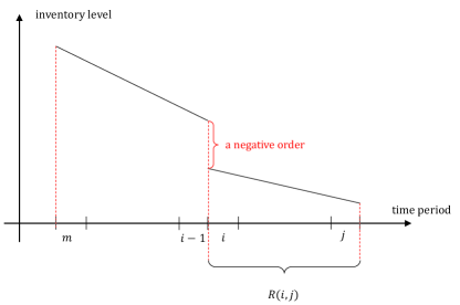
Figure 2: A negative order takes place in period $i$.

The final relaxation model is presented as follows. This relaxation determines the expected order quantity by decision variables $\tilde{S}_{t}$ and $\tilde{I}_{t}$.

$$\min\quad \displaystyle\sum_{k=t}^{T}[\delta_{k}\cdot K+z(\tilde{S}_{k}-\tilde{I}_{k-1})+h\cdot\tilde{H}_{k}+b\cdot\tilde{B}_{k}],$$ (16)

s.t. $$\delta_{k}=0\rightarrow\tilde{I}_{k}+\tilde{d}_{k}-\tilde{I}_{k-1}=0, k=t,\ldots,T,$$

$$P_{j,k}\geq\delta_{j}-\sum\limits_{r=j+1}^{k}\delta_{r}, k=t,\ldots,T,\mathop{}j=t,\ldots,k,$$

$$\sum\nolimits_{j=t}^{k}P_{j,k}=1, k=t,\ldots,T,$$

$$P_{j,k}=1\rightarrow\tilde{H}_{k}=\hat{\mathcal{L}}(\tilde{I}_{k}+\tilde{d}_{j,k},d_{j,k}), k=t,\ldots,T,\mathop{}j=t,\ldots,k,$$

$$P_{j,k}=1\rightarrow\tilde{B}_{k}=\mathcal{L}(\tilde{I}_{k}+\tilde{d}_{j,k},d_{j,k}), k=t,\ldots,T,\mathop{}j=t,\ldots,k,$$

$$\tilde{H}_{k},\tilde{B}_{k}\geq 0,\quad P_{j,k},\delta_{k}\in\{0,1\}, k=t,\ldots,T,\mathop{}j=t,\ldots,k.$$

By summing the expected costs of various replenishment cycles, the problem is relaxed into a multi-stage newsvendor problem with non-stationary stochastic demand (Petruzzi and Dada,, 1999). However, the piecewise linear approximation is less efficient in large-scale instances with non-normally distributed demand. For example, Ma et al., (2022) provide details on its extension to non-stationary Poisson demand. The next subsection presents a shortest-path formulation of this problem and discusses how to handle negative orders in the optimal solution.

3.2 An equivalent shortest path formulation

Tarim, (1996) show that the shortest path problem provides a valid lower bound for the non-relaxed formulation, as a solution of the relaxed problem presented in Section 3.1. The shortest path problem can be efficiently solved by Dijkstra’s algorithm (Cormen et al.,, 2001, pp. 595-–601) in $\mathcal{O}(n^{2})$ time, where $n$ is the number of nodes in the shortest-path graph.

Consider an acyclic network $\mathcal{G}=(\mathcal{V},\mathcal{E})$ with a set of nodes $\mathcal{V}=\{1,2,\ldots,T+1\}$ denoting periods, where $T$ is the planning horizon length, and the dummy $T+1$ is introduced as the final node (boundary condition) to indicate the end of planning horizon. Each arc $(i,j)\in\mathcal{E}$ has an associated cost $c_{i,j}$ which denotes the expected cost of replenishment cycle $R(i,j-1)$, where

$$c_{i,j}=c(y-x)+L_{i,j-1}(y),$$ (17)

and $x$ is the opening inventory level of cycle $R(i,j-1)$, $y$ is the inventory level after replenishment,

$$L_{i,j-1}(y)=h\mathbb{E}[\max(y-d_{i,j-1},0)]+b\mathbb{E}[\max(d_{i,j-1}-y,0)].$$ (18)

where $d_{i,j-1}$ is a random variable, representing the cumulative demand over the horizon ($i,j-1$). For any generic demand distribution,

$$\mathbb{E}[\max(d_{i,j-1}-y,0)]=\int_{d_{i,j-1}}^{\infty}(d_{i,j-1}-y)\varphi(d_{i,j-1})\mathrm{d}d_{i,j-1}$$ (19)

applying the first order loss function on the scalar $y$ and the random variable $d_{i,j-1}$, and

$$\mathbb{E}\max(y-d_{i,j-1},0)=\int_{y=0}^{\xi}(y-d_{i,j-1})\varphi(d_{i,j-1})\mathrm{d}d_{i,j-1}$$ (20)

applying the complementary first order loss function.

Therefore, entries $c_{i,j}$ formulate a connection matrix with the expected cost of replenishment cycles $R(i,j-1)$, and the problem can be modelled as a one-way temporal feasibility problem (Wagner and Whitin,, 1958), illustrated in Figure 3. We also note that for any node $t\in\mathcal{V}$, the decision of placing replenishment ($\delta_{t}=1)$ is represented by an outbound arc. We refer this problem as “ESP $\mathcal{G}=(\mathcal{V},\mathcal{E})$”.

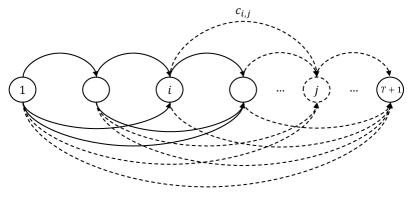
Figure 3: Shortest path problem:

solid lines represent actual arcs in the graph,
and dotted lines indicate arcs connecting through omitted nodes.

Let $\mathcal{G}^{*}=(\mathcal{V}^{*},\mathcal{E}^{*})\subseteq\mathcal{G}$ denote the optimal solution (the shortest path) out of all possible combinations of replenishment cycles and associated costs. $\mathcal{G}^{*}$ indicates a set of consecutive disjoint replenishment cycles that satisfies the demand in the planning horizon with a minimum expected total cost. The selected replenishment cycle $R(i,j-1)$ is indicated by arc $(i,j)\in\mathcal{E}^{*}$.

Under the constraints of the feasibility to the original (non-relaxed) problem, no negative order should be assigned to any replenishment cycle in the optimal solution; in other words, for any two consecutive replenishment cycles in the optimal solution $R(k,i-1)$ and $R(i,j-1)$, $\tilde{S}_{i}^{*}\geq\tilde{I}_{i-1}^{*}$ should hold. Otherwise, it means a negative replenishment order occurs, implying the solution is optimal for the relaxed problem but not feasible for the original problem. Therefore, we propose a repetitive augmenting procedure to resolve the infeasibility.

4 A repetitive augmenting procedure for infeasibility

Once the shortest-path problem is formulated and solved, as previously described, it becomes straightforward to ascertain whether the optimal solution adheres to all constraints. If the optimal replenishment plan does not include any negative order quantities, then the solution is both feasible and optimal for the original problem. Conversely, if the solution is infeasible due to the inclusion of negative replenishment quantities, we employ a repetitive augmentation procedure to rectify this infeasibility. This section details the methodology used to determine the optimal solution in scenarios where the initial solution is infeasible.

4.1 Filtering by Principle of Optimality

In this paper, when a negative replenishment order is detected in the shortest-path solution, we initiate a method to resolve the infeasibility, which needs to be implemented on the full graph constructed by the equivalent shortest-path formulation. The shortest-path problem satisfies the Principle of Optimality, which states that any subpath of an optimal path is itself optimal. Leveraging this principle, we can eliminate redundant paths to reduce the problem without affecting the optimal solution. Therefore, as the first step of the algorithm, we apply a filtering procedure to reduce the graph structure by removing unnecessary arcs that cannot be part of any optimal path.

Specifically, for any $2\leq k\leq T$ and for a sequence of nodes $(i_{1},i_{2}),(i_{2},i_{3}),\ldots,(i_{k},i_{k+1})\in\mathcal{E}$, if the cumulative cost of travelling from node $i_{1}$ to $i_{k+1}$ directly is lower than or equal to the sum of travelling through each intermediate node $i_{2},i_{3},\ldots,i_{k}$, i.e.,

$$\sum_{m=i_{1}}^{k}c_{i_{m},i_{m+1}}\leq c_{i_{1},i_{k+1}},$$ (21)

then arc $(i_{1},i_{k+1})$ is redundant and will be removed from the graph. In the context of the graph-based algorithm, this filtering step effectively prunes the graph by eliminating edges that do not contribute to potential optimal paths, leading to lower computational requirements in subsequent stages of the algorithm.

4.2 An augmenting procedure to resolve infeasibility

Regarding the filtered graph $\mathcal{G}_{f}$, Dijkstra’s algorithm can subsequently be applied to identify the shortest path. As stated in Section 3.2, the final optimal solution is confirmed if it passes the feasibility check. However, if any node $i$ in the optimal solution satisfies $\tilde{S}_{i}<\tilde{I}_{i-1}$, indicating a negative replenishment order, this constitutes an infeasibility that must be rectified to ensure the solution is both practical and implementable.

The augmenting procedure is designed to address negative replenishment orders that signify infeasibilities in the inventory path. A negative order implies that the preceding cycle replenished too much inventory, leading to an excess that needs adjustment. For nodes where negative orders occur, additional nodes and arcs are introduced to reshape the replenishment cycles. The core idea is to merge the cycle containing the negative replenishment order $R(i,j)$ into a preceding cycle $R(m,i)$. Consider a new replenishment cycle $\hat{R}(m,j-1)\triangleq R(m,i-1)+R(i,j-1)$, where period $m$ is the start of the replenishment cycle which ends at period $i$ where the negative replenishment order occurs. In the graph view, $R(m,i-1)$ is the latest replenishment cycle connecting to node $i$ with an infeasible inbound arc, and the negative order takes place at the beginning of period $i$, as illustrated by Figure 4.

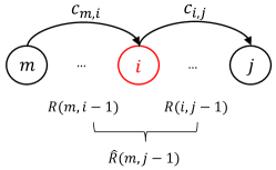
Figure 4: The relation between replenishment cycles, arcs and cost associated with arcs.

The augmentation incorporates the overstocked period $R(i,j)$ into the earlier cycle $R(m,i)$, thereby reducing the initial inventory level for the combined cycle. As illustrated in Figure 5, a new path is formed by connecting the inventory levels between the two cycles, and this ensures that the inventory conservation constraint is maintained and the negative order is eliminated.

This approach involves restructuring the graph by duplicating nodes and creating alternative paths that ensure all replenishment quantities are non-negative. By redirecting the inventory flow through the newly introduced nodes, the algorithm adjusts the path structure to eliminate infeasibilities. As a result, the augmented graph is re-solved to obtain a feasible and near-optimal inventory policy that maintains consistency across the planning horizon while satisfying the problem’s constraints. This new replenishment cycle will pay the ordering cost twice:

1. at the beginning of period $m$, $K+zQ_{m}$ will be incurred as usual; and

2. at the beginning of period $i$, $K$ will be incurred, representing a charge to review the inventory level even though an order with quantity zero occurs.

Therefore, the calculation of the new opening inventory level for period $m$ (denoted by $\hat{S}_{m}$) involves determining the optimum of a multi-period Newsvendor problem over periods $m$ to $i$; according Eq.(17) and (18), its expected cost is

$$\hat{c}_{m,i}\triangleq K+c_{m,i}.$$ (22)

To incorporate one more time period $i$ in the new replenishment cycle $R(m,i)$, the optimum (i.e. the optimal opening inventory level) remains the same as the optimal order-up-to level over periods $m$ to $i$ in the original graph. In fact, due to the convexity of the expected cost function of the multi-period Newsvendor problem, the addition of fixed ordering cost $K$ does not change the derivative, thus the optimum remains the same. And this applies to the subsequent periods $i+1,\ldots,j$ and associated new replenishment cycles $\hat{R}(m,i+1),\ldots,\hat{R}(m,j)$. Figure 6 illustrates the rectified expected total cost for the situation in Figure 5.

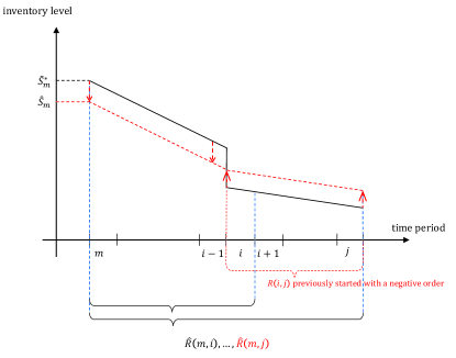
Figure 5: The elimination of the negative order: inventory-level view.

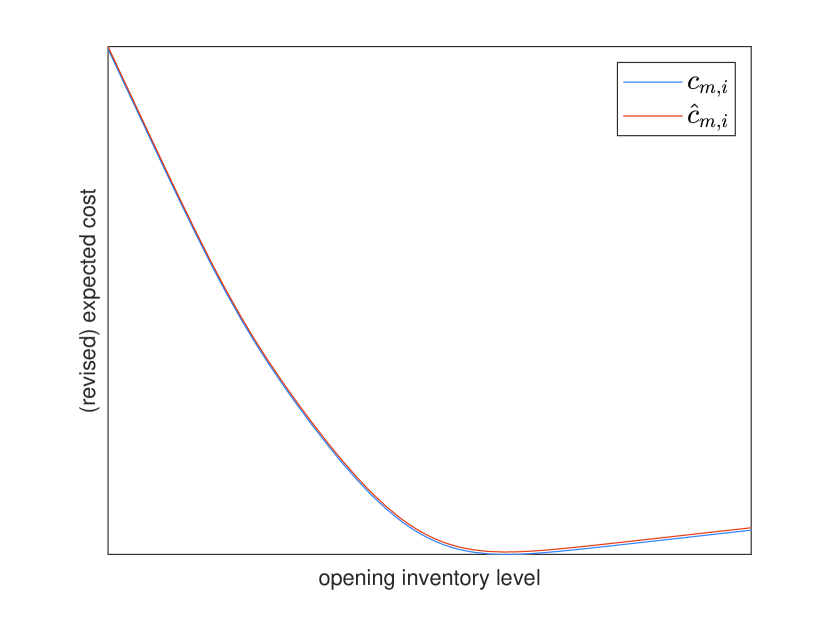
(a) ETC of the multi-period Newsvendor problem with/without additional $K$.

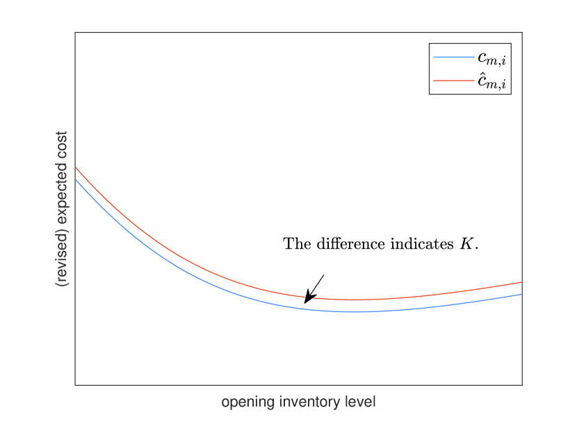
(b) ETC of the multi-period Newsvendor problem with/without additional $K$ (zoomed in).

Figure 6: The elimination of the negative order: expected-total-cost (ETC) view: Unchanged optimum of the multi-period Newsvendor problem with additional $K$.

Building on this logic, we propose the augmenting procedure indicated by Figure 7: to re-direct, duplicate and re-compute.

• Re-direct. Introduce a new node $i^{\prime}$ and connect node $m$ with node $i^{\prime}$. Node $i$ can be deleted if it is not included in any other existing arc.

• Duplicate. Connect the new node $i^{\prime}$ with node $j+2,\ldots,T+1$ with the order-up-to levels and closing inventory levels unchanged from node $i$. These arcs represent identical replenishment cycles $R(i,j+1),\ldots,R(i,T+1)$ as ESP $\mathcal{G}$.

• Re-compute. Introduce the new arc $[i^{\prime},i+1],\ldots,[i^{\prime},j+1]$, denoted by the dash-dotted line. If these arcs contribute to a solution, then new replenishment cycles $\hat{R}(m,i),\ldots,\ldots,\hat{R}(m,j)$ are independently considered stand-alone without the involvement of arc ($m,i^{\prime}$). In other words, the dash-dotted line represents an independent replenishment cycle starting from the node connecting with the newly created node $i^{\prime}$ (node $m$ in the case of Figure 7). And the expected cost $\hat{c}_{m,k}$ ($k=i,\dots,j$) associated with the new replenishment cycle can be computed according to Eq.(22). We create notations $\hat{S}(m,k)$ and $\hat{I}_{k}$ to denote the optimal order-up-to level and expected closing inventory for replenishment cycles $\hat{R}(m,k)$ ($k=i,\dots,j$).

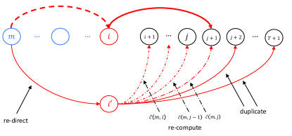
Figure 7: Augmentation for infeasible scenarios.

For the convenience of notations, for any arc ($i,j+1$), we apply the pair $(\hat{S}(i,j),\hat{I}_{i,j})$ to denote the expected opening inventory level and the expected closing inventory at the end of period $j$; in the case of dash-dotted line via an introduced node $i^{\prime}$, the pair is associated with the replenishment cycle $\hat{R}(m,j)$, where $m$ is the latest connected node to node $i^{\prime}$.

4.3 A repetitive algorithm

For the replenishment cycle $\hat{R}(m,j)$ via the newly introduced node $i^{\prime}$, the opening inventory level $\hat{S}_{m}$ is modified to incorporate the additional periods included in the new cycle. Let $\tilde{S}_{m}$ represent the opening inventory level derived from the original graph $\mathcal{G}$. Typically, it holds that $\tilde{S}_{m}\geq\hat{S}_{m}$, as illustrated in Figure 5. This difference in inventory levels potentially impacts the feasibility between $\tilde{I}_{m-1}$ and $\hat{S}_{m}$, necessitating a repetitive augmentation procedure to ensure continuity and feasibility across the replenishment cycles. Following this, when $\hat{R}(m,j)$ is formed, we assess the feasibility for all connecting nodes preceding node $m$. If a feasibility violation is detected, the augmenting procedure is re-applied to address these discrepancies.

The pseudo-code for determining the shortest path (optimal inventory planning) is presented in Algorithm 1. Algorithm 1 initiates by filtering the original graph $\mathcal{G}$ from the relaxed problem, wherein cost-inefficient arcs – typically those spanning a large number of periods – are removed. Applying Dijkstra’s Algorithm, the shortest path $\mathcal{G}^{*}$ can be determined. For every node $i\in\mathcal{G}^{*}$, a feasibility check is conducted on each inbound arc. For an inbound arc $(m,i)$ with the expected closing inventory $\tilde{I}_{i-1}$ and for each outbound arc $(i,j)$ with $\tilde{S}_{i}$, the condition $\tilde{I}_{i-1}\leq\tilde{S}_{i}$ is checked. If this condition is satisfied for every inbound-outbound pair, then the inbound arc $(m,i)$ is preserved at node $i$. Otherwise, if a violation occurs indicating a potential negative order, the augmenting procedure is applied repetitively until all arcs, whether original or augmented, satisfy the feasibility criteria.

Algorithm 1 Arc augment procedure to compute the optimal replenishment for the non-stationary lot-sizing problem under ($R_{t},S_{t}$) policy.

1:Input: the shortest path problem graph $\mathcal{G}=(\mathcal{V},\mathcal{E})$.

2:Output: the optimal inventory planning $\widetilde{\bm{S}}^{*}$ and $\bm{\delta}^{*}$.

3:$\mathcal{G}_{f}=(\mathcal{V}_{f},\mathcal{E}_{f})$ $\leftarrow$ $\mathcal{G}=(\mathcal{V},\mathcal{E})$.

4:for $2\leq k\leq T$ and ($i_{1},i_{2}$), ($i_{2},i_{3}$), $\ldots$, ($i_{k},i_{k+1}$) and $(i_{1},i_{k+1})\in\mathcal{E}$ do

5:    if $\sum_{m=i_{1}}^{k}c_{i_{m},i_{m+1}}\leq c_{i_{1},i_{k+1}}$ then

6:        then $\mathcal{E}_{f}\leftarrow\mathcal{E}_{f}\backslash(i_{1},i_{k+1})$.

7:    end if

8:end for

9:Apply Dijkstra’s Algorithm to obtain the shortest path $\mathcal{G}^{*}=(\mathcal{V}^{*},\mathcal{E}^{*}).$

10:for node $i=1,\ldots,T\in{\mathcal{V}^{*}}$ do

11:    for node $m<i$ do

12:        if $\tilde{I}_{i-1}>\tilde{S}_{i}\text{ for the replenishment cycle }R(i,j)\text{, where }j\geq i+1$ then

13:           introduce node $i^{\prime}$ and update the graph $\mathcal{V}^{*}\leftarrow\mathcal{V}^{*}\bigcup\{i^{\prime}\}$;

14:           create arc ($m,i^{\prime}$), update the graph $\mathcal{E}^{*}\leftarrow\mathcal{E}\bigcup\{(m,i^{\prime})\}$;

15:           create arc $(i^{\prime},j+2),\ldots,(i^{\prime},T+1)$ by duplication, update the graph $\mathcal{E}^{*}\leftarrow\mathcal{E}^{*}\bigcup\{(i^{\prime},j+2),\ldots,(i^{\prime},T+1)\}$;

16:           create arc $[i^{\prime},i+1],\ldots,[i^{\prime},j+1]$ and replenishment cycle $\hat{R}(m,i),\ldots,\hat{R}(m,j)$, compute $\hat{c}_{m,i},\ldots,\hat{c}_{m,j}$ according to Eq.(22), derive $\hat{S}(m,k)$ and $\hat{I}_{k}$ ($k=i,\dots,j$), and update the graph $\mathcal{E}^{*}\leftarrow\mathcal{E}^{*}\bigcup\{[i^{\prime},i+1],\ldots,[i^{\prime},j+1]\}$;

17:        end if

18:        for node $p=1,\ldots,m-1$ do

19:           if $\tilde{I}_{p}>\hat{S}_{m}$ for $R(m,k)$, where $k=i,\dots,j$  then

20:               break and continue with line 10.

21:           end if

22:        end for

23:    end for

24:end for

25:Apply Dijkstra’s Algorithm and the updated shortest path $\mathcal{G}^{*}$, extract the optimal expected order-up-to level $\widetilde{S}_{t}^{*}$.

26:for $t=1,\ldots,T$ do

27:    $\delta_{i}^{*}=1$ if node $i\in\mathcal{V}^{*}$.

28:end for

5 An illustrative example

We consider the instance presented in Rossi et al., (2011, sec.7) with 95% $\alpha$ service level, while we refer to the definition $\frac{b}{b+h}=\alpha=0.95$ to have $b=19$ when $h=1$ for the penalty scheme. Demand in each period is independent and follows the Normal distribution with means $\tilde{d}_{t}=\{100,125,25,40,30\}$ and the coefficient of variation $\sigma_{t}/\tilde{d}_{t}=0.3$. We apply a fixed ordering cost $K=50$ and unit ordering cost $z=0$.

We first apply 12 partitions to the approximated optimal ($R_{t},S_{t}$) policy according to Rossi et al., (2014) with piecewise linear approximation and obtain the expected total cost of 446.7 with 500,000 simulations. The inventory system with this policy is illustrated in Figure 8.

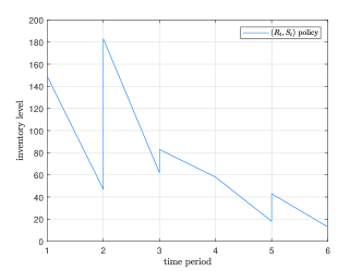
Figure 8: Expected inventory levels by ($R_{t},S_{t}$) policy with piecewise linear approximation.

Secondly, we remove a flow balance constraint to allow negative orders and solve a relaxed ($R_{t},S_{t}$) policy, which leads to an expected cost $444$ by 500,000 simulations. The problem is then formulated as the graph shown in Figure 9, where the expected costs of replenishment cycles are presented on arcs. The optimal path $1\rightarrow 2\rightarrow 3\rightarrow 4\rightarrow 6$ generates an ($R_{t},S_{t}$) policy with the expected total cost as 437.5 by 500,000 simulations. Figure 10 illustrates the ($R_{t},S_{t})$ policies solved by piecewise linear approximation and shortest path, where a negative order can be noticed at the beginning of period 3 by both methods.

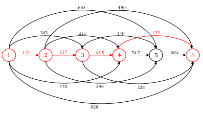
Figure 9: The optimal path for 5-period instance with expected costs of replenishment cycles.

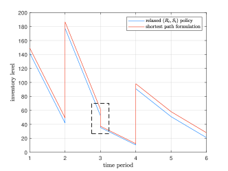
Figure 10: Expected inventory levels by relaxed ($R_{t},S_{t}$) policy with piecewise linear approximation and shortest path formulation. A negative order quantity is observed in period 3.

To resolve the infeasibility, the repetitive augmentation procedure is applied. We obtain the filtered graph as Figure 11 and augmented graph as Figure 12, which solves the shortest path as $1\rightarrow 2\rightarrow 3^{\prime}\rightarrow 5\rightarrow 6$, which leads to an ($R_{t},S_{t}$) policy with the expected total cost as 447.5 by 500,000 simulations. Details of implementing the augmented procedure can be found in Appendix B.

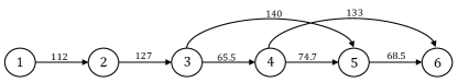
Figure 11: Filtered graph with expected costs.

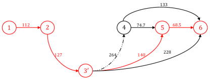
Figure 12: Optimal path of Example 1 with repetitive augmenting procedure.

Figure 13 illustrates the augmented graph without the application of any filtering procedure. Comparing with Figure 12, it is evident that the filtering procedure significantly reduces computational effort by avoiding the introduction of two potential new nodes, $3^{\prime}$ and $5^{\prime}$ ($3^{\prime\prime}$ indicates node $3^{\prime}$ in Figure 12). The optimal path, as revealed in both figures, remains unchanged.

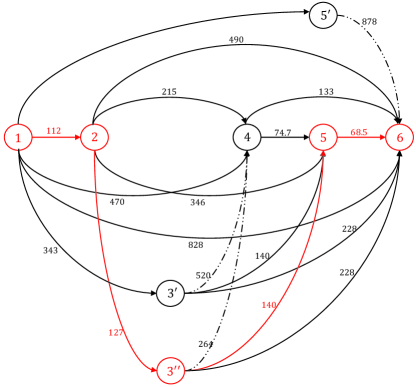
Figure 13: Optimal path of Example 1 with the augmenting procedure with no filtration.

6 Computational study

This section presents a comprehensive computational analysis aimed at evaluating the proposed graph-based algorithm outlined in Section 4.3 for addressing non-stationary stochastic demand within a penalty cost framework. The purpose of the analysis is three-fold.

1. How does the proposed graph-based algorithm compare with state-of-the-art formulations in the literature in terms of computational efficiency?

2. How does the occurrence of negative orders affect the decision’s reliability?

3. How does the proposed graph-based algorithm scale with increasing planning horizons in terms of computational time?

For the first question, we benchmark the computational performance of the graph-based algorithm against the results obtained by Tunc et al., (2018), the most recent research that emphasises computational efficiency in handling non-stationary demand while effectively minimising holding and backorder costs in the $(R,S)$ inventory system. The proposed graph-based algorithm integrates relaxations that decompose the problem into order cycles, which are subsequently optimised based on the expected cycle costs. This approach yields computational advantages, especially in instances with high demand variability. Therefore, the comparison primarily examines the computational runtime. Specifically, the analysis aims to demonstrate that the proposed algorithm performs competitively, or even outperforms the benchmark, in terms of runtime while maintaining solution quality.

According to Eq.(19) and (20), the graph-based algorithm can accommodate any demand distribution through numerical integration. Integrals can be computed using open-source libraries such as Apache Commons Math (‘UnivariateIntegrator’) in Java and SciPy (‘scipy.integrate’) in Python. However, these approaches can be time-consuming, particularly when applied to high-dimensional problems or large data sets. To mitigate the impact of integrations on efficiency, closed-form expressions can be used when available. In the computational analysis presented, we focus on the Normal distribution, which allows us to leverage its closed-form solutions for the integrals (Rossi et al.,, 2014):

$$\mathcal{L}(x,\xi)=\sigma\left(\varphi\left(\frac{x-\mu}{\sigma}\right)-\left(1-\Phi\left(\frac{x-\mu}{\sigma}\right)\right)\frac{x-\mu}{\sigma}\right)$$ (23)

and

$$\hat{\mathcal{L}}(x,\xi)=\sigma\left(\varphi\left(\frac{x-\mu}{\sigma}\right)+\Phi\left(\frac{x-\mu}{\sigma}\right)\frac{x-\mu}{\sigma}\right),$$ (24)

where $x$ is an arbitrary scalar variable and $\xi$ a Normally distributed random variable with mean $\mu$ and standard deviation $\sigma$; $\varphi(\cdot)$ and $\Phi(\cdot)$ are density and cumulative function, respectively, for the standard Normal distribution $N(0,1)$. The application of these closed-form formulas can significantly reduce computational time for preparation without compromising the accuracy of the results, emphasising the comparison of the algorithm’s computational efficiency.

The second question focuses on evaluating how the occurrence of negative orders impacts the reliability of decisions derived by the graph-based algorithm. We acknowledge that (1) if no negative order occurs in the shortest path, the graph-based algorithm’s solution aligns with the optimal or exact cost, affirming its reliability without the need for further adjustments; and (2) the presence of negative orders in the shortest path indicates infeasibility, suggesting the need for augmentation. Thus, we first assess the frequency of negative orders in the shortest path solution. For scenarios where negative orders are present, we then compare the expected total costs before and after the repetitive augmentation to quantify the impact of negative orders on overall cost and evaluate the effectiveness of the augmentation in mitigating infeasibilities.

The third question examines the scalability of the graph-based algorithm by evaluating its performance on extended planning horizons. This analysis aims to assess whether the algorithm remains computationally efficient and continues to deliver high-quality solutions as the planning horizon increases.

Therefore, in this computational study, we first conduct experiments on the test bed adopted from Tunc et al., (2018) (Set-A) to evaluate performance under various parameter settings. Holding costs are fixed at $h=1$ across all experiments, with three setup costs $K=\{225,900,2500\}$, and penalty costs $b=\{2,5,10\}$. We consider three lengths of planning horizon $N=\{20,30,40\}$, and demand is assumed to follow a normal distribution with three coefficient of variation values $\rho=\{0.1,0.2,0.3\}$. Two demand patterns are considered:

1. Erratic: Mean are drawn uniformly from $[0,100]$; and

2. Lumpy: Mean are drawn from $[0,420]$ with probability 0.2, and from $[0,20]$ with probability 0.8.

For each combination of the planning horizon and demand pattern, we generate 10 random instances, resulting in a total of 1620 test instances in this test set.

Additionally, we conduct an extended analysis with planning horizons of 50, 75, and 100 periods, using the same demand patterns and cost parameter configurations. This extended test set also includes 1620 instances, allowing us to investigate the scalability of the algorithm.

All computations are performed in JAVA 1.8.0_201 by 4.0 (1.90+2.11) gigahertz Intel(R) Core(TM) i7-8650U CPU with 16.0 gigabytes of RAM.

Table 1 presents the occurrence of negative orders in the shortest path. No negative orders were observed in the erratic demand pattern throughout the entire experiment. In contrast, all 195 instances with one or more negative orders were associated with the lumpy demand pattern. As the planning horizon extends, the number of instances with negative orders increases from 58 to 73, indicating that longer planning horizons lead to a higher frequency of infeasible solutions. The standard deviation parameter $\rho$, which indicates the variability of the demand, also shows a strong influence. An increase in $\rho$ for the same set of demand means directly leads to an increase in the variability of actual demand, causing a rise in negative order instances from 16 to 110. The penalty cost $b$ affects the occurrence of negative orders; as $b$ rises from 2 to 10, the number of instances increases from 33 to 93. This trend suggests that higher penalty costs encourage the algorithm to maintain higher inventory levels to avoid backorders. In fact, increasing the penalty cost can result in overstocking, making it difficult to balance inventory between consecutive cycles. Consequently, closing inventory levels may exceed subsequent opening levels, which leads to more frequent negative orders in the results.

Table 1: Occurrence of negative order(s) in the shortest path pivoting parameters.

Problem Settings	Number of instances with negative order in the shortest path
Erratic	0
Lumpy	195
$T=20$	58
30	64
40	73
$\rho=0.1$	16
0.2	69
0.3	110
$b=2$	33
5	69
10	93
$K=225$	156
900	39
2500	0
Total	195

Table 2 reports the average computation times for different stages of the graph-based algorithm under various demand patterns and parameter settings. The preparation time in the first column refers to the time required to populate the expected cycle costs for different possible opening inventory levels in order to build the connection matrix. For this test set, a range up to $4\tilde{d}_{1,N}$ was used for the opening inventory levels, where $\tilde{d}_{1,N}$ represents the total sum of demand means over the entire planning horizon, with a step size of 1 unit chosen for practical significance. Specifically, this range was selected to ensure sufficient coverage of potential inventory levels without compromising computational efficiency, and under such conditions, the solution is guaranteed to reach a globally optimal result numerically. The results show that the preparation time is primarily influenced by the length of the planning horizon. This outcome is expected, as a longer planning horizon results in a larger connection matrix, requiring more time to populate all potential inventory levels and compute the expected cycle costs accordingly. The second column shows that the time required to solve the shortest path is considerably small, measured in milliseconds, despite minor variations.

The third column shows that the repetitive augmentation can efficiently repair the solution when negative orders are present. The computation time for this stage increases with the length of the planning horizon and with the penalty cost, while it decreases with the fixed ordering cost. For the erratic demand pattern or instances with $K=2500$, no negative orders are observed, resulting in zeros in the table. Overall, when no negative orders are present, the entire algorithm (including preparation and shortest-path stages) solves in an average time of 1.590 seconds; for instances with negative orders, the average solution time is 4.699 seconds.

Compared with the results reported by Tunc et al., (2018), who achieved lower average computational times of 3.39 seconds for similar problem instances (see Table 1 in (Tunc et al.,, 2018)), our method shows higher computational times in absolute terms. Although our method has larger computation times, its overall efficiency is demonstrated by its ability to handle different demand patterns and effectively resolve negative orders. Therefore, we can answer question 1 by confirming that, while our method involves a higher preparation time, especially due to building the connection matrix, it remains efficient overall.

Table 2: Average computation times (s) under different demand patterns and pivoting parameters.

Problem Settings	Preparation time	Solving shortest path	Implementing filtration, repetitive augmentation and re-optimise (if any)
Erratic	1.318	0.00014	0.000
Lumpy	1.860	0.00015	3.109
$T=20$	0.162	0.00012	1.645
30	0.921	0.00011	2.376
40	3.685	0.00021	4.916
$\rho=0.1$	1.634	0.00036	3.362
0.2	1.592	0.00003	3.024
0.3	1.543	0.00005	3.126
$b=2$	1.645	0.00029	1.747
5	1.567	0.00008	2.949
10	1.556	0.00007	3.711
$K=225$	1.598	0.00032	3.117
900	1.554	0.00004	3.078
2500	1.617	0.00008	0.00
Average	1.590	0.00015	3.109

Table 3 addresses question 2 by examining how the occurrence of negative orders influences the reliability of decisions in terms of total cost deviations. Firstly, if a solution contains no negative orders, it is guaranteed to be the exact optimal solution, indicating maximum reliability. Therefore, fewer negative orders imply better decision quality. The first column presents the number of negative orders in the shortest path before augmentation, and it aligns with trends from Table 1, confirming that the planning horizon length, the standard deviation parameter $\rho$, the penalty cost $b$, and the fixed ordering cost $K$ significantly affect the occurrence of infeasibility. On average, 341 negative orders occur in the shortest path across the entire set of problem instances.

To resolve these negative orders, the algorithm introduces additional nodes, as shown in the second column. The total number of introduced nodes reflects the frequency of negative orders, with 989 nodes added on average. The trend shows that more nodes are needed for longer planning horizons and higher values of $b$, whereas increasing $K$ leads to fewer required nodes.

Most importantly, the reliability of the augmented solution is measured by the percentage increase in expected total cost (third column). This difference represents the additional cost incurred to resolve negative orders and restore feasibility. On average, for instances with negative orders, the total cost increases by 3.56%. This cost increase is particularly notable for shorter planning horizons and low $\rho$ values, which imply that frequent augmentations may lead to higher deviations in expected costs.

Table 3: Evaluation of the repetitive procedure under different demand patterns and pivoting parameters.

Problem Settings	Total number of negative orders in shortest path without augmentation	Total number of introduced nodes in repetitive algorithm	Difference in expected total cost (%)
Erratic	0	0	0
Lumpy	341	989	3.56
$T=20$	83	175	2.72
30	118	345	3.36
40	140	469	4.42
$\rho=0.1$	18	77	4.53
0.2	100	320	3.75
0.3	223	592	3.30
$b=2$	36	56	3.32
5	125	337	3.31
10	180	596	3.84
$K=225$	300	819	3.44
900	41	170	4.08
2500	0	0	0
Average	341	989	3.56

Table 4 addresses question 3 by reporting the average computational time for each stage of the graph-based algorithm applied to the larger test set. Despite the increased complexity in the test set, the results demonstrate that the algorithm remains computationally efficient even for large-scale instances. Among 1,620 instances in total, 232 instances encountered negative replenishment orders in the shortest-path solution for their relaxed problem. On average, the proposed algorithm obtained results in 158.27 seconds for instances without negative orders and 169.61 seconds for those requiring repetitive augmentations. Note that the extended preparation time stems from constructing the connection matrix for the graph; a line search was applied to ensure accuracy, contributing to the longer preparation time. This likely represents an upper bound on computational time, with the potential for reduction through alternative methods such as binary search. This result highlights the algorithm’s capability to handle complex, large-scale problems while maintaining low computational costs. The inclusion of the filtration and re-optimisation process, averaging only 10.84 seconds, further underlines the method’s ability to efficiently resolve infeasibilities and adapt to more challenging problem settings.

Table 4: Average computation times (s) under different demand patterns and pivoting parameters for long planning horizon instances.

Problem Settings	Number of instances with negative order in the shortest path	Preparation time	Solving shortest path	Implementing filtration, repetitive augmentation and re-optimise (if any)
Erratic	0	178.15	0.00043	0.00
Lumpy	232	138.39	0.00026	10.84
$T=50$	70	11.29	0.00012	6.09
75	78	73.83	0.00024	11.94
100	84	389.68	0.00068	13.79
$\rho=0.1$	18	132.77	0.00061	5.97
0.2	85	208.51	0.00018	13.65
0.3	129	133.53	0.00024	9.67
$b=2$	46	170.67	0.00055	3.90
5	74	171.17	0.00025	9.86
10	112	132.97	0.00023	14.35
$K=225$	183	175.57	0.00053	11.80
900	49	172.39	0.00024	7.25
2500	0	126.85	0.00027	0.00
Average	232	158.27	0.00034	10.84

7 Conclusion

This paper developed a graph-based approach for solving single-item, single-location inventory lot-sizing problems under non-stationary stochastic demand with ($R_{t},S_{t}$) policy and penalty cost scheme. The method relaxed the original ($R_{t},S_{t}$) MILP model and obtained an equivalent shortest-path problem, which is then used to determine the optimal order-up-to levels. The infeasibility from the relaxation is captured as negative orders, which is resolved by a repetitive augmenting procedure including the steps of filtration, augmentation and re-optimisation.

The computational experiments confirm the efficiency and effectiveness of the proposed approach across various demand patterns and parameter configurations. The reliability of the graph-based algorithm is influenced by the occurrence of negative replenishment orders. Among the 1,620 test instances, 195 required augmentation due to the presence of negative orders, primarily observed in scenarios with high penalty costs, long planning horizons, low fixed ordering costs, and high demand variability. On average, addressing these infeasibilities results in a 3.56% increase in expected total costs compared to the relaxed solution. Although the presence of negative orders increases computational complexity, the repetitive augmentation procedure effectively adjusts the relaxed solution to eliminate infeasibilities, ensuring that the final policy provides a reliable and practical solution for non-stationary stochastic demand problems.

In terms of computational efficiency, the graph-based algorithm is benchmarked against the method proposed by Tunc et al., (2018). Although their method demonstrates a shorter average computation time of 3.39 seconds, the proposed approach achieves competitive performance by accommodating a broader range of problem settings. Specifically, our algorithm determines the final inventory policy within an average of 1.590 seconds for instances without negative replenishment orders and 4.699 seconds for those requiring repetitive augmentation.

The scalability of the graph-based algorithm is demonstrated with the larger-scale test set, maintaining computational efficiency by averaging 158.27 seconds for problems without negative orders and 169.61 seconds when repetitive augmentations were needed. The augmentation and re-optimisation processes resolve infeasibilities in an average of 10.84 seconds, showing the algorithm’s ability to handle increasing complexity in a reasonable computational time.

Future research should focus on determining an exact upper bound for computational efficiency under diverse problem scales and demand patterns. Moreover, extending the algorithm to alternative inventory control strategies, such as the $(s,Q)$ policy, would enable broader applicability to accommodate variable order quantities for managing static-dynamic uncertainty in inventory systems.

Appendix A Notations

Table A1: Notations of important functions

Functions	Explaination
$L_{t}(y)$	expected immediate holding and penalty cost when the inventory level after replenishment is $y$ at period $t$, $L_{t}(y)=h\mathbb{E}[\max(y-d_{t},0)]+b\mathbb{E}[\max(d_{t}-y,0)]$.
$\tilde{I}_{t}$	expected closing inventory level of period $t$, $\tilde{I}_{t}=\tilde{H}_{t}-\tilde{B}_{t}$.
$\tilde{H}_{t}(y)$	expected holding inventory level at the end of period $t$, $\tilde{H}_{t}(y)=\mathbb{E}[\max(y-d_{t},0)]$
$\tilde{B}_{t}(y)$	expected back-ordered inventory level at the end of period $t$, $\tilde{B}_{t}(y)=\mathbb{E}[\max(d_{t}-y,0)]$.
$C_{t}(x)$	expected total cost over periods $t$ to $T$, starting from inventory level $x$.
$R(i,j)$	the replenishment cycle starting from period $i$ and terminates at the end of period $j$.
$\hat{R}(i,j)$	the augmented replenishment cycle starting from period $i$ and terminates at the end of period $j$, via a newly introduced node by the augmentation between $i$ and $j$.
$\tilde{S}_{t}$	the expected order-up-to level at the beginning of period $t$.
$\hat{S}_{t}$	the expected order-up-to level at the beginning of period $t$ for the replenishment cycle $\hat{R}(t,\cdot)$.
$d_{i,j-1}$	the cumulative demand over the horizon ($i,j-1$)
$c_{i,j}$	the expected cost of replenishment cycle $R(i,j-1)$ for arc $(i,j)\in\mathcal{E}$, $c_{i,j}=c(y-x)+L_{i,j-1}(y)$.
$i$	node $i$, represents the beginning of a period $i$, $i=1,2,\ldots,T+1$, where node $T+1$ indicates the end of the planning horizon.
$(i,j)$	arc $(i,j)$, represents the replenishment cycle $R(i,j-1)$.
$[i,j]$	arc $[i,j]$, formulated by augmenting procedure, represents the replenishment cycle $\hat{R}(i,j)$ via a newly introduced node by augmentation between $i$ and $j$.
$\hat{c}_{m,i}$	the expected cost of $\hat{R}(m,i-1)$, $\hat{c}_{m,i}=K+c_{m,i}.$

Appendix B Implementing revised augmenting procedure on Example 1 by periods.

Figure B1 presents the expected costs of all potential replenishment cycles.

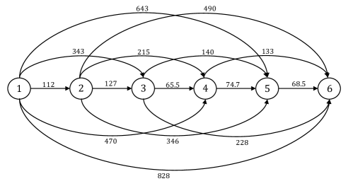
Figure B1: Paths constructed by the shortest path problem with expected costs.

Applying the filtering procedure, Figure B1 is reduced to Figure B2, with expected closing and opening inventory levels in Figure B3. And we start the feasibility check from this point.

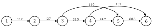
Figure B2: Filtered graph with expected costs.

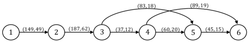
Figure B3: Filtered graph with expected opening and closing inventory levels.

According to the algorithm, for every node from 1 to 5, we check inbound arcs with the expected closing inventory level and the order-up-to levels. We set the initial inventory level as 0 and assume that an order is always placed at the beginning of period 1. So all outbound arcs are preserved for node 1 at this stage.

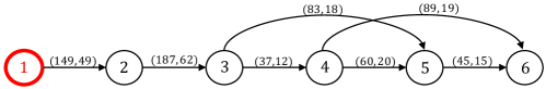
Figure B4: Feasibility check for node 1.

For node 2, 1 inbound arc is observed: (1,2) with the expected closing inventory level 49; and 1 outbound arcs are observed, where (2,3) with the order-up-to level $187>49$. Feasibility holds.

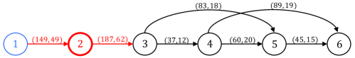
Figure B5: Feasibility check for node 2.

For node 3, 1 inbound arcs are observed: (2,3) with the expected closing inventory 62. And 2 outbound arcs are observed: (3,4) with order-up-to level 37, (3,5) with order-up-to level 83. We notice that the infeasibility appears on (2,3) - (3,4) with $\tilde{I}_{2}=62$ = 62 and $\tilde{S}_{3}=37$. Therefore, the augmenting procedure is applied.

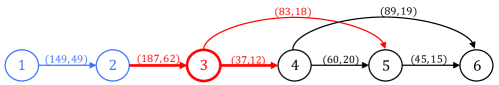
Figure B6: Feasibility check for node 3 - infeasibility found.

First, we create node 3’ and connect it with node 1 to create (1,3’). Now periods 2 and 3 are included in the same order cycle, but the second ordering cost will be charged due to the presence of new node 3’. Implement multi-period Newsvendor calculation, the replenishment cycle (2,3’,4), i.e. $\hat{R}(2,4)$, denoted by arc [2,4], has the optimal order-up-to level 203.3237, the expected cost 264.9488, and the expected closing inventory level = 53.3144. For the subsequent nodes, we duplicate arcs (3’,5) and (3’,6).

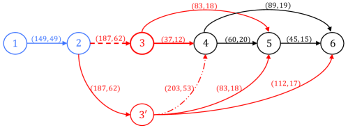
Figure B7: Augmentation for node 3.

The removal of the arc $(2,3)$ results in the disconnection of node $3$ from the graph, along with the introduction of replacement arcs $(3^{\prime},5)$ and $(3^{\prime},6)$. Consequently, the original node $3$ is rendered redundant and can be removed from the graph. At this point, it is also necessary to assess whether this modification should be repeated. The feasibility of this configuration is verified through examining arcs $(1,2)$ and $[2,4]$. Specifically, with $\tilde{I}_{1}=49<203=\hat{S}_{4}$ for $\hat{R}(2,4)$, the current setup is validated as feasible, allowing the process to proceed without further immediate modifications.

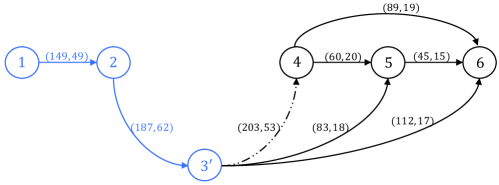
Figure B8: Augmented graph and feasibility check for new arc [2,4], denoted by dash-dotted line.

For node 4, the inbound arcs (3’,4) and the outbound arcs (4,5) and (4,6) have been evaluated and found not to cause any infeasibility; thus, no augmentation is necessary for this node. The same holds true for node 5 and 6, where both the inbound and outbound arcs maintain feasibility without the need for additional modifications.

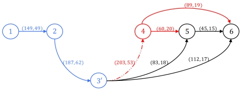
Figure B9: Feasibility check for node 4.

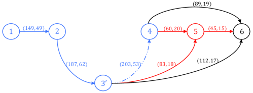
Figure B10: Feasibility check for node 5.

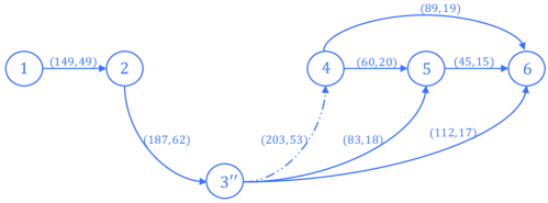
Figure B11: Feasibility check for node 6.

Applying Dijkstra’s Algorithm, the shortest path can be found in Figure B12 with expected costs illustrated in Figure B13

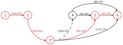
Figure B12: Optimal path with expected opening and closing inventory levels.

Figure B13: Optimal path with expected costs.

References

- Bellman, (1957) Bellman, R. (1957). Dynamic Programming. Princeton University Press, Princeton, NJ, USA.
- Belotti et al., (2016) Belotti, P., Bonami, P., Fischetti, M., Lodi, A., Monaci, M., Nogales-Gómez, A., and Salvagnin, D. (2016). On handling indicator constraints in mixed integer programming. Computational Optimization and Applications, 65(3):545–566.
- Bookbinder and Tan, (1988) Bookbinder, J. H. and Tan, J.-Y. (1988). Strategies for the probabilistic lot-sizing problem with service-level constraints. Management Science, 34(9):1096–1108.
- Cormen et al., (2001) Cormen, T. H., Leiserson, C. E., Rivest, R. L., and Stein, C. (2001). Introduction to algorithms second edition. The Knuth-Morris-Pratt Algorithm.
- De Kok and Inderfurth, (1997) De Kok, T. and Inderfurth, K. (1997). Nervousness in inventory management: comparison of basic control rules. European Journal of Operational Research, 103(1):55–82.
- Harris, (1913) Harris, F. W. (1913). How many parts to make at once. Operations Research, 38(6):947–950.
- Ma et al., (2022) Ma, X., Rossi, R., and Archibald, T. W. (2022). Approximations for non-stationary stochastic lot-sizing under ()-type policy. European Journal of Operational Research, 298(2):573–584.
- Özen et al., (2012) Özen, U., Doğru, M. K., and Tarim, S. A. (2012). Static-dynamic uncertainty strategy for a single-item stochastic inventory control problem. Omega, 40(3):348–357.
- Petruzzi and Dada, (1999) Petruzzi, N. C. and Dada, M. (1999). Pricing and the newsvendor problem: A review with extensions. Operations research, 47(2):183–194.
- Rossi et al., (2015) Rossi, R., Kilic, O. A., and Tarim, S. A. (2015). Piecewise linear approximations for the static–dynamic uncertainty strategy in stochastic lot-sizing. Omega, 50:126–140.
- Rossi et al., (2011) Rossi, R., Tarim, S. A., Hnich, B., and Prestwich, S. (2011). A state space augmentation algorithm for the replenishment cycle inventory policy. International Journal of Production Economics, 133(1):377–384.
- Rossi et al., (2014) Rossi, R., Tarim, S. A., Prestwich, S., and Hnich, B. (2014). Piecewise linear lower and upper bounds for the standard normal first order loss function. Applied Mathematics and Computation, 231:489–502.
- Scarf, (1960) Scarf, H. (1960). The optimality of () policies in the dynamic inventory problem.
- Tarim, (1996) Tarim, S. A. (1996). Dynamic lotsizing models for stochastic demand in single and multi-echelon inventory systems. PhD thesis, Lancaster University.
- Tarim et al., (2011) Tarim, S. A., Dogru, M. K., Özen, U., and Rossi, R. (2011). An efficient computational method for a stochastic dynamic lot-sizing problem under service-level constraints. European Journal of Operational Research, 215(3):563–571.
- Tarim and Kingsman, (2004) Tarim, S. A. and Kingsman, B. G. (2004). The stochastic dynamic production/inventory lot-sizing problem with service-level constraints. International Journal of Production Economics, 88(1):105–119.
- Tarim and Kingsman, (2006) Tarim, S. A. and Kingsman, B. G. (2006). Modelling and computing (, ) policies for inventory systems with non-stationary stochastic demand. European Journal of Operational Research, 174(1):581–599.
- Tempelmeier, (2007) Tempelmeier, H. (2007). On the stochastic uncapacitated dynamic single-item lotsizing problem with service level constraints. European Journal of Operational Research, 181(1):184–194.
- Tunc et al., (2014) Tunc, H., Kilic, O. A., Tarim, S. A., and Eksioglu, B. (2014). A reformulation for the stochastic lot sizing problem with service-level constraints. Operations Research Letters, 42(2):161–165.
- Tunc et al., (2018) Tunc, H., Kilic, O. A., Tarim, S. A., and Rossi, R. (2018). An extended mixed-integer programming formulation and dynamic cut generation approach for the stochastic lot-sizing problem. INFORMS Journal on Computing, 30(3):492–506.
- Wagner and Whitin, (1958) Wagner, H. M. and Whitin, T. M. (1958). Dynamic version of the economic lot size model. Management science, 5(1):89–96.
- Wemmerlöv, (1989) Wemmerlöv, U. (1989). The behavior of lot-sizing procedures in the presence of forecast errors. Journal of Operations Management, 8(1):37–47.