Likelihood & Correlation Analysis of Compton Form Factors for Deeply Virtual Exclusive Scattering on the Nucleon

Abstract

A likelihood analysis of the observables in deeply virtual exclusive photoproduction off a proton target, $ep\rightarrow e^{\prime}p^{\prime}\gamma^{\prime}$, is presented. Two processes contribute to the reaction: deeply virtual Compton scattering, where the photon is produced at the proton vertex, and the Bether-Heitler process, where the photon is radiated from the electron. We consider the unpolarized process for which the largest amount of data with all the kinematic dependences are available from corresponding datasets with unpolarized beams and unpolarized targets from Jefferson Lab. We provide and use a method which derives a joint likelihood of the Compton form factors, which parametrize the deeply virtual Compton scattering amplitude in QCD, for each observed combination of the kinematic variables defining the reaction. The unpolarized twist-two cross section likelihood fully constrains only three of the Compton form factors (CFFs). The impact of the twist-three corrections to the analysis is also explored. The derived likelihoods are explored using Markov chain Monte Carlo (MCMC) methods. Using our proposed method we derive CFF error bars and covariances. Additionally, we explore methods which may reduce the magnitude of error bars/contours in the future.

I Introduction

The process of deeply virtual Compton scattering (DVCS), where an electron scatters coherently off a proton target producing a hard photon, is deemed the most accurate probe of the nucleon quark and gluon distributions in coordinate space. The latter can be extracted from the non-forward QCD matrix elements between the initial ($p$) and final ($p^{\prime}$) proton, known as generalized parton distributions (GPDs), through Fourier transformation with respect to the proton momentum transfer ($\Delta=p-p^{\prime}$). Assuming the validity of QCD factorization, one can parametrize the DVCS amplitude in terms of several Compton form factors (CFFs), which arise from the various allowed beam-target polarization configurations. CFFs are convolution integrals of GPDs with known kernels/coefficient functions. GPDs can therefore be inferred, although only indirectly, from the experimental observation of CFFs (we refer the reader to reviews on the subject in Diehl (2001); Belitsky and Radyushkin (2005); Kumericki et al. (2016) and references therein).

DVCS holds a unique role among all deeply virtual exclusive scattering (DVES) experiments since, through the interference with the background Bethe Heitler (BH) process, where the final state hard photon is radiated from the electron, one can extract the CFFs directly at the amplitude level. Furthermore, because of the presence of only one distinct hadronic blob, deeply virtual electron photoproduction is a clean probe, as compared to deeply virtual exclusive meson production, or to similar processes with more than one hadron in the final state, where an additional non leading dependence on the QCD scale, $Q^{2}$, is more likely to contaminate a QCD-based analysis. Notwithstanding, a quantitative determination of CFFs, and consequently of GPDs, from DVCS data has been notoriously difficult, and no definitive result exists to date on the dominance of the asymptotic regime that should be manifested at $t/Q^{2}\rightarrow 0$, with $t=\Delta^{2}$. A major hurdle in the analysis to extract GPDs from experiment arises due to the presence of two inverse problems: a first one for the extraction of the various CFFs from data, and a subsequent one concerning the extraction of GPDs from CFFs.

In this paper we present results of a joint multivariate Bayesian likelihood analysis of unpolarized electron scattering off an unpolarized proton target using a subset of the available DVCS data which displays a full kinematic dependence in all variables, i.e. which is not integrated over the azimuthal angle, $\phi$. Our aim is to place quantitative bounds on the experimental extraction of CFFs. We define the unknown CFFs as parameters and we first assume that their kinematic coefficients, as well as the proton elastic form factors from the BH amplitude are exactly calculable in a QCD framework. We have used all unpolarized DVCS data for our analysis which consequently displays full covariance in our results. In this respect, we are adopting what could be considered as a “brute force”, or completely unbiased method. The first and foremost goal of this analysis is to answer the questions: are present data consistent with QCD? Is there enough evidence in the data to validate a QCD-based description of deeply virtual exclusive processes? Are present experimental data following trends expected in the asymptotic regime, or are higher twist terms dominant? What further methods would be appropriate for testing the QCD nature of the cross section?

In the $t/Q^{2}\rightarrow 0$ limit, the QCD evolution of GPDs is expected to proceed analogously as for the parton distribution functions (PDFs) and distribution amplitude (DAs) from inclusive deep inelastic scattering experiments, i.e. in a collinear framework, generating $Q^{2}$ dependent logarithmic corrections. There is only a technical point of departure from PDFs and DAs given by the fact that the kernels of the evolution equations, as well as the next-to-leading order Wilson coefficient functions, also depend on the GPDs’ skewness variable, $\xi$, measuring the longitudinal momentum fraction difference between the initial and final struck particles, besides the standard longitudinal parton momentum fraction $x$. Departures from the parton model-based description, parametrized in QCD by twist-two GPDs, could originate kinematically as target mass corrections, as well as dynamically, due to the exchange of gluons between the struck quark and the spectator system, and to coherent phenomena possibly including multi-quark scattering, resonance production, and scattering from constituent mesons. All of these phenomena are potential higher twist effects displaying characteristic $Q^{2}$ inverse powers dependence.

By illustrating several issues that arise for the specific dataset analyzed here, we are seeking to establish a statistical framework and a general procedure that can be subsequently applied to all DVES-type data. The paper is organized as follows: in Section II we give a theoretical description of the cross section using a QCD-based formulation up to twist-three terms, as a point of reference. We introduce the main motivation of our analysis, which is that the present DVCS cross section data allows equivalently good fits with completely different CFFs. We subsequently introduce a systematic approach that allows us to address the several open questions stemming from the result of using a simple fitting procedure, including: how many form factors can be extracted from data, and what are their boundaries? How can the given theoretical background be validated? The quantitative methods to address these questions require a full-fledged multivariate likelihood analysis and they are described in Section III; in Section IV we present and discuss the numerical results of this analysis, addressing the question of whether the data are interpretable in a QCD context including the contributions of higher twists. The conclusions and outlook are given in Section V.

II Theoretical Framework and Motivation

The exclusive photon electroproduction process $ep\rightarrow e^{\prime}p^{\prime}\gamma^{\prime}$ can occur either through deeply virtual Compton scattering (DVCS) or through the Bethe-Heitler (BH) process (see Fig. 1).

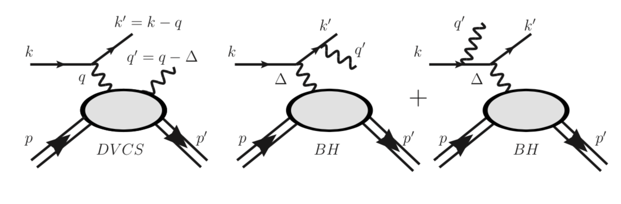
Figure 1: Leading order diagrams for exclusive photon electro-production $ep\rightarrow ep\gamma$. The DVCS process is parametrized by GPDs, while the Bethe-Heitler background process is parametrized by elastic form factors.

The latter are summed coherently at the amplitude level, giving rise to the following differential cross section

$$\frac{d^{4}\sigma}{dx_{Bj}dQ^{2}dtd\phi}\equiv\sigma_{TOT}=\sigma_{BH}+\sigma_{DVCS}+\sigma_{\mathcal{I}},$$ (1)

where $\sigma_{BH}$ and $\sigma_{DVCS}$ are the Bethe-Heitler and DVCS contributions, respectively, while $\sigma_{\mathcal{I}}$ is the cross section resulting from their interference. In Eq.(1), the cross section is written in terms the kinematic variables $(s,Q^{2},x_{Bj},t,\phi)$, where

• $s=(k+p)^{2}$ is the electron-proton center of mass energy squared,

• $Q^{2}=-(k-k^{\prime})^{2}=-q^{2}$ is the four-momentum transfer squared between the incoming and outgoing electrons,

• $x_{Bj}=Q^{2}/2(pq)$ is Bjorken-$x$. In the asymptotic limit, disregarding $t/Q^{2}$ and $M^{2}/Q^{2}$ corrections, $x_{Bj}$ is written in terms the skewness parameter, $\xi=-(\Delta q)/[(pq)+(p^{\prime}q)]=x_{Bj}/(2-x_{Bj})$

• $t=(p-p^{\prime})^{2}=(q^{\prime}-q)^{2}$ is the four-momentum transfer squared between the initial and final protons ($q^{\prime}$ is the final photon four-momentum),

• $\phi$ is the azimuthal angle between the planes defined by the electron momenta, by the final proton, $p^{\prime}$, and photon, $q^{\prime}$.

In this paper we will focus on unpolarized electrons scattering off an unpolarized proton, therefore the cross section does not depend on an additional azimuthal angle stemming from the proton spin orientation. (Note that Kriesten et al. (2020) writes the five-fold differential cross section, which includes the transverse spin angle $\phi_{S}$, while Eq. (1) is integrated over $\phi_{S}$. Therefore, the $\Gamma$ factor used in the expressions following Eq. (1) has an extra factor of $2\pi$ compared to the $\Gamma$ factor in Kriesten et al. (2020, 2022a); Kriesten and Liuti (2022). In this case, the BH contribution to the cross section is parametrized in terms of the proton Dirac and Pauli elastic form factors $F_{1}(t)$ and $F_{2}(t)$, as follows Kriesten et al. (2020),

$$\sigma_{BH}=\frac{\Gamma}{t}\,\bigg{\{}A_{BH}\left[F_{1}^{2}(t)+\tau F_{2}^{2}(t)\right]+B_{BH}\,\tau\left[F_{1}(t)+F_{2}(t)\right]^{2}\bigg{\}}\,,$$ (2)

where $\tau=-t/4M^{2}$, $M$ being the proton mass. The pre-factor, $\Gamma$, includes the Jacobian for the change of variables in going from the final state particles’ momenta to the invariants defined above, and it is expressed as Kriesten et al. (2020),

$$\Gamma=\frac{\alpha^{3}(2\pi)}{16\pi^{2}(s-M^{2})^{2}\sqrt{1+\gamma^{2}}\,x_{Bj}},$$ (3)

where $\alpha$ is the electromagnetic fine structure constant, and $\gamma^{2}=4M^{2}x_{Bj}^{2}/Q^{2}$. The coefficients $A_{BH},B_{BH}$ are dimensionless functions of the kinematic variables $(s,Q^{2},x_{Bj},t,\phi)$ that were calculated in Kriesten et al. (2020) (we present them for completeness in Appendix A). The nucleon elastic form factors are known precisely in a wide kinematic range (for more details, see the review Punjabi et al. (2015) an references therein), and various parametrizations for them exist in the literature Kelly (2004); Bradford et al. (2006); Brash et al. (2002). The BH contribution is therefore considered a known term that we will subtract out from the data in our analysis.

Assuming a QCD factorized framework, the DVCS contribution is described by four complex Compton form factors (CFFs) at leading order: $\mathcal{H}$, $\mathcal{E}$, $\widetilde{\mathcal{H}}$ and $\widetilde{\mathcal{E}}$, which correspond to the various allowed quark-proton polarization configurations in the proton. Information regarding the 3D partonic structure of nucleons is encoded in the QCD correlation functions that define the generalized parton distributions (GPDs) Ji (1997a); Radyushkin (1997); Müller et al. (1994) (for comprehensive reviews of GPDs and DVCS we refer the reader to Diehl (2003); Belitsky and Radyushkin (2005); Kumericki et al. (2016)). In a nutshell, GPDs depend on the longitudinal momentum fraction, $x$, on the momentum transfer, $t$, between the initial and final proton – allowing us to access the quark and gluon transverse spatial distribution through Fourier transformationDiehl (2002); Burkardt (2003); Soper (1977) – and on the skewness parameter, $\xi$. The second Mellin moments of the GPDs in the variable $x$, are directly related to the form factors parametrizing the QCD energy momentum tensor, whose matrix elements between proton states describe orbital angular momentum, pressure, and the shear forces, that emerge from the proton’s quark and gluon internal dynamics Ji (1997b); Polyakov (2003); Shanahan and Detmold (2019); Lorcé et al. (2021). GPDs enter the DVCS amplitude in convolutions with perturbative QCD Wilson coefficient functions, giving the CFFs,

$$\begin{split}\mathcal{F}(\xi,t,Q^{2})&=\sum_{q}e_{q}^{2}\int_{-1}^{+1}dx\left[\frac{1}{\xi-x-i\epsilon}-\frac{1}{\xi+x-i\epsilon}\right]F^{q}(x,\xi,t,Q^{2})\\ \widetilde{\mathcal{F}}(\xi,t,Q^{2})&=\sum_{q}e_{q}^{2}\int_{-1}^{+1}dx\left[\frac{1}{\xi-x-i\epsilon}+\frac{1}{\xi+x-i\epsilon}\right]\widetilde{F}^{q}(x,\xi,t,Q^{2})\end{split}$$ (4)

where $F^{q}=\{H^{q},E^{q}\}$, $\widetilde{F}^{q}=\{\widetilde{H}^{q},\widetilde{E}^{q}\}$, and $e_{q}$ is the fractional charge of the quark $q$ (analogous expressions can be written for gluons).

Using the covariant helicity amplitude formalism described in detail in Kriesten et al. (2020) with the virtual photon, $q$, on the negative $z$-axis Diehl and Sapeta (2005), the expression for the unpolarized cross section at leading twist in this formalism is written as (see also Kriesten and Liuti (2022); Kriesten et al. (2022a); Almaeen et al. (2022, 2024))

$$\sigma_{DVCS} = \frac{\Gamma}{Q^{2}(1-\epsilon)}\Bigg{\{}2(1-\xi^{2})\bigg{(}\left[{\Re e\mathcal{H}}(x_{Bj},t,Q^{2})\right]^{2}+\left[{\Im m\mathcal{H}}(x_{Bj},t,Q^{2})\right]^{2}+\big{[}{\Re e\widetilde{\mathcal{H}}}(x_{Bj},t,Q^{2})\big{]}^{2}+\big{[}{\Im m\widetilde{\mathcal{H}}}(x_{Bj},t,Q^{2})\big{]}^{2}\bigg{)}$$ (5)

$$+ \frac{t_{0}-t}{2M^{2}}\bigg{(}\left[{\Re e\mathcal{E}}(x_{Bj},t,Q^{2})\right]^{2}+\left[{\Im m\mathcal{E}}(x_{Bj},t,Q^{2})\right]^{2}+\big{[}\xi\,{\Re e\widetilde{\mathcal{E}}(}x_{Bj},t,Q^{2})\big{]}^{2}+\big{[}\xi\,{\Im m\widetilde{\mathcal{E}}}(x_{Bj},t,Q^{2})\big{]}^{2}\bigg{)}$$

$$- 4\xi^{2}\bigg{(}{\bf\Re e\mathcal{H}}(x_{Bj},t,Q^{2})\,{\Re e\mathcal{E}}(x_{Bj},t,Q^{2})+{\Im m\mathcal{H}}(x_{Bj},t,Q^{2})\,\Im m\mathcal{E}(x_{Bj},t,Q^{2})+{\Re e\widetilde{\mathcal{H}}}(x_{Bj},t,Q^{2})\,{\Re e\widetilde{\mathcal{E}}}(x_{Bj},t,Q^{2})$$

$$+ {\Im m\widetilde{\mathcal{H}}(}x_{Bj},t,Q^{2})\,{\Im m\widetilde{\mathcal{E}}}(x_{Bj},t,Q^{2})\bigg{)}\Bigg{\}},$$

where

$$\epsilon=\frac{1-y-\frac{1}{4}y^{2}\gamma^{2}}{1-y+\frac{1}{2}y^{2}+\frac{1}{4}y^{2}\gamma^{2}},$$ (6)

with $y=(pq)/(pk)=Q^{2}/(x_{Bj}s)$, is the ratio of the longitudinal to transverse virtual photon polarization evaluated in the $M^{2}/Q^{2}<<1$ limit, and $t_{0}=-4M^{2}\xi^{2}/(1-\xi)$. The following remarks are in order:

1. the leading order DVCS contribution is a quadratic expression of all four complex CFFs corresponding to eight unknowns (we call all eight terms “CFFs”, for brevity);

2. since the unpolarized case involves only helicity amplitudes for a transversely polarized virtual photon whose phases cancel when multiplied with their complex conjugates, the expression in Eq.(5) is independent of the azimuthal angle, $\phi$;

3. the cross section depends on $s$ only through the overall factor, $\Gamma/Q^{2}(1-\epsilon)$.

Figure 2: The coefficients $A^{\mathcal{I}}_{UU},B^{\mathcal{I}}_{UU},C^{\mathcal{I}}_{UU}$ as a function of $\phi$ for the kinematic bin $E_{b}=10.591$ GeV, $x_{Bj}=0.369$, $Q^{2}=4.53\,\text{GeV}^{2}$, $t=-0.2094\,\text{GeV}^{2}$. Note that these coefficients are dimensionless. They do not depend upon the compton form factors.

The BH-DVCS interference contribution, $\sigma_{\cal I}$, is dependent on $\phi$ and reads,

$$\sigma_{\mathcal{I}} = \frac{\Gamma}{Q^{2}}\bigg{\{}A_{\mathcal{I}}\,\left[F_{1}(t)\,{\bf\Re e\mathcal{H}}(x_{Bj},t,Q^{2})+\tau\,F_{2}(t)\,{\bf\Re e\mathcal{E}}(x_{Bj},t,Q^{2})\right]+B_{\mathcal{I}}\,[F_{1}(t)+F_{2}(t)]\,{\bf\Re e}\left[{\bf\mathcal{H}}(x_{Bj},t,Q^{2})+{\bf\mathcal{E}}(x_{Bj},t,Q^{2})\right]$$ (7)

$$+ C_{\mathcal{I}}[F_{1}(t)+F_{2}(t)]\,{\bf\Re e}\widetilde{\bf\mathcal{H}}(x_{Bj},t,Q^{2})\bigg{\}}.$$

The kinematic coefficients $A_{\mathcal{I}}$, $B_{\mathcal{I}}$, $C_{\mathcal{I}}$, in Eq.(7) are dimensionless functions of the kinematic variables $(s,Q^{2},x_{Bj},t,\phi)$; they have been calculated in Kriesten et al. (2020, 2022a); Kriesten and Liuti (2022); for completeness, we present their expressions in Appendix B. An example of their dependence on $\phi$ is shown for a particular kinematic bin in Figure  2. Other kinematic bins show a similar behavior, with a clear dominance of $A_{\mathcal{I}}$ over $B_{\mathcal{I}}$ and $C_{\mathcal{I}}$. For the present analysis it is important to notice that:

1. the interference term is parametrized by only three unknowns given by the real parts of the CFFs: $\Re e\mathcal{H}$, $\Re e\mathcal{E}$, and $\Re e\widetilde{\mathcal{H}}$, which enter the equation linearly in a form which closely tracks the elastic cross section parametrization into form factors Sofiatti and Donnelly (2011);

2. The $\phi$ dependence factorizes: it resides entirely in the kinematic coefficients which are clearly separated from the $\phi$-independent CFFs.

The $\phi$-dependent structure of $\sigma_{DVCS}$ and $\sigma_{\cal I}$, outlined above, is important in the method that we will employ to extract CFFs from DVCS data in the following Sections. An example of the various contributions to the cross section is shown in Figure 3.

Figure 3: The expected relative contributions of the DVCS, BH, and interference terms to the total cross section, Eq.(1), in a particular kinematic bin. The DVCS and interference terms are calculated using the parametrization developed in Goldstein et al. (2013); Kriesten et al. (2022b); experimental data from Georges et al. (2022); Georges (2018). In the plot the CFF values are fixed as: ReH = -1.7927, ReE = -1.9572, ReHt = 3.1316, ReEt = 3.3615, ImH = -1.9528, ImE = -0.7543, ImHt = -0.6698, ImEt = -4.2128,

Motivation

In this paper we will not be concerned with the inverse problem of extracting GPDs from CFFs, but with the very first step of extracting CFFs from experimental data. As we explain below, the eight unknowns given by the real and imaginary parts of the proton CFFs (Eq.(4)), can determine the shape of a curve fit through the cross section data at a given kinematic bin. These eight unknowns describing the cross section at leading order can vary considerably for each kinematic bin. In Figure 4 we show, for illustration, what happens if one performs a curve fit allowing seven of them to vary but fixing $\Re eE$ to substantially different values chosen to be: $[-25,0,50]$. We can see how we obtain excellent fits for all three fixed values, with comparable $\chi^{2}$ per d.o.f. values. However, we can also show that once $\Re eE$ is fixed, $\Re eH$ and $\Re e\widetilde{H}$ become well constrained. It turns out that we are in the regime of bounded, but (statistically) covariant results for 3/8 twist-2 CFFs, which we present later in Section IV. This result, which motivates our study, can be formalized using a likelihood analysis on each kinematic bin as explained in detail in Section III.

Figure 4: Illustration of how the DVCS cross section data ($\sigma_{UU}\equiv\sigma_{TOT}$ in Eq.(1), $\phi$ in radians) allows good fits with wildly different CFFs. For the particular kinematic bin shown here $\Re eE$ is set to each of [-25, 0, 50] and subsequently a fit is performed. The other seven twist-two CFFs are allowed to vary. The corresponding curve fits are all in excellent agreement with the data. Visually one can see the variation between the three curves is negligible compared to the width of the error bars on the data. Quantitatively we also confirm the negligible visual difference by calculating the $\chi^{2}$.

Finally, we also provide a preliminary analysis including the extra sixteen Compton form factors which appear in cross section at twist-three Kriesten and Liuti (2022). As we explain in what follows, the DVCS contribution in unpolarized scattering will no longer be independent of $\phi$. The impact of a twist-three analysis of CFFs from DVCS data will be discussed in Section IV. Developing a strategy to include twist-three terms will be important as more data become available other approaches are given in Refs Belitsky et al. (2002); Braun et al. (2014); Belitsky and Mueller (2010), which can differ significantly beyond the leading order (for a detailed discussion see Kriesten and Liuti (2022)).

II.1 Experimental Data

For this analysis we have chosen to use the unpolarized DVCS data from the Jefferson Lab Hall A Collaboration Georges et al. (2022); Georges (2018), with the kinematic parameters $[E,x_{Bj},Q^{2},t,\phi]$. For convenience, we are working with the dataset published on the Gepard GitHub page Kumerički (2022) under the name BSS HALLA - 18. The reason for using this dataset is due to its binning; each bin has 24 datapoints of different $\phi$ with identical values of the other four parameters, which lends itself well to the analysis described in Section III.

$E_{beam}$ (GeV)	$x_{Bj}$	$Q^{2}$ $({\rm GeV}^{2})$	$t$ $({\rm GeV}^{2})$	$\phi$ (deg)	$\sigma_{total}$	$\Delta\sigma$
10.591	0.369	4.53	-0.2094	7.5	0.01394	0.00058
10.591	0.369	4.53	-0.2094	22.5	0.01292	0.00056
10.591	0.369	4.53	-0.2094	37.5	0.01305	0.00056
10.591	0.369	4.53	-0.2094	52.5	0.01216	0.00054
10.591	0.369	4.53	-0.2094	67.5	0.01147	0.00052
10.591	0.369	4.53	-0.2094	82.5	0.01128	0.00051
10.591	0.369	4.53	-0.2094	97.5	0.00875	0.00046
10.591	0.369	4.53	-0.2094	112.5	0.00915	0.00046
10.591	0.369	4.53	-0.2094	127.5	0.00904	0.00045
10.591	0.369	4.53	-0.2094	142.5	0.00838	0.00044
10.591	0.369	4.53	-0.2094	157.5	0.00828	0.00044
10.591	0.369	4.53	-0.2094	172.5	0.00798	0.00043
10.591	0.369	4.53	-0.2094	187.5	0.00774	0.00043
10.591	0.369	4.53	-0.2094	202.5	0.00841	0.00045
10.591	0.369	4.53	-0.2094	217.5	0.00853	0.00045
10.591	0.369	4.53	-0.2094	232.5	0.00991	0.00049
10.591	0.369	4.53	-0.2094	247.5	0.00969	0.00049
10.591	0.369	4.53	-0.2094	262.5	0.01021	0.00049
10.591	0.369	4.53	-0.2094	277.5	0.01093	0.00051
10.591	0.369	4.53	-0.2094	292.5	0.01223	0.00054
10.591	0.369	4.53	-0.2094	307.5	0.01236	0.00054
10.591	0.369	4.53	-0.2094	322.5	0.01382	0.00057
10.591	0.369	4.53	-0.2094	337.5	0.01543	0.00061
10.591	0.369	4.53	-0.2094	352.5	0.01376	0.00058

Table 1: Experimental data of the unpolarized DVCS cross section from Jefferson Lab Hall A Georges et al. (2022); Georges (2018) in 1 single kinematic bin used for our likelihood analysis. This table corresponds to various single bin likelihood analysis figures shown in this paper 5 6 7. The full available dataset contains 44 such kinematic bins. The summary of likelihood results for all kinematic bins is included in Table 3 and Figure 8.

The data were taken after the Jefferson Lab beam energy upgrade to 12 GeV, and the energy spans the values $4.487\text{ GeV}\leq E\leq 10.992\text{ GeV}$. The other kinematic variables span the ranges $2.71\text{ GeV}^{2}\leq Q^{2}\leq 8.51\text{ GeV}^{2}$, $0.363\leq x_{\text{Bj}}\leq 0.617$ and $0.2094\text{ GeV}^{2}\leq-t\leq 1.3732\text{ GeV}^{2}$. For this kinematic regime the values of $\sqrt{-t/Q^{2}}$ range between 0.2 and 0.5, so we can expect some contamination from the twist-3 contribution.

The published experimental data contains statistical uncertainties, as well as two types of systematic uncertainties, correlated and uncorrelated. The uncorrelated systematic uncertainties affect each experimental bin individually, while the correlated ones affect all bins equally. The uncorrelated uncertainties are ascribed to the contamination of background processes, most prominently semi-inclusive deep inelastic scattering (SIDIS), and the reported values of the uncertainties are between 2% and 5%. The correlated uncertainties come from several aspects of the analysis and the experimental setup, and their values range between 3% and 6%. These uncertainties depend on the kinematic bin, but also on the value of $\phi$. In all bins, the statistical uncertainties range between 3% and 4%, and their $\phi$ dependence is ignored. In this work we decided to only consider the statistical uncertainties because the systematic uncertainties have not been fully evaluated for this measurement. The authors report an average correlated uncertainty of 3%, but, as mentioned above, estimate that it can go up to 6%. For more details, see Georges (2018).

III Deriving a likelihood function

We will use two different versions of a Bayesian likelihood analysis to place bounds upon the Compton form factors (CFFs). We denote the first version as “canonical” as it is simpler as we can ultimately write the total joint likelihood of the parameters of interest as a simple product of Gaussians. The second version is more complicated as it involves taking the differences of two total cross sections at different $\phi$ angles, and calculating a corresponding covariance matrix for the differences calculated. The first version is easier to understand but the second method provides tighter bounds on the CFFs. The reason for the tighter bounds can be intuitively understood by realizing the same information is used in both versions, but the first allows four parameters to vary, while the second only has three parameters. A model with fewer parameters can be more tightly constrained using the same information as another with more parameters. It is then illustrative to show that both methods provide similar results and we can view the simpler method as a reasonable sanity check to the more complicated method.

For both versions, we assume that the data can be randomly selected from a normal distribution. If the model of the cross section was perfect and the measurements had no error we would expect

$$\sigma_{model}(\phi)=\sigma_{exp}(\phi)$$

However, the observations do have error thus we can view each cross section measurement as independent and sampled from a true value calculated from the model $\mu=\sigma_{model}$.

In what follows we give a detailed description of each of the two likelihood analysis approaches, and show their results in Section IV.

III.1 Canonical Likelihood

The canonical method’s likelihood can be written as a product of gaussians. For a fixed set of kinematic parameters $[E,x_{Bj},Q^{2},t]$, the total cross section is measured at 24 azimuthal $\phi$ angles (we show an example of the dataset in Table 1), and can be also separately calculated using a phenomenological model. In this work we use the model from Ref.Kriesten et al. (2020); Kriesten and Liuti (2022). Assuming our model is correct, the calculated cross sections will still differ from the observed cross sections. The difference between model and observation must be explained by the error bars (measurement error). Such error bars are reported by the experiment and are available in the observed data table from Kumerički (2022), discussed in section II.1. For a single datapoint (one $\phi$ value), the probability that the model differs from an observation is described by a univariate Gaussian probability density function. Thus using such a univariate Gaussian, we compare cross section observed ($d^{4}\sigma_{exp}\equiv x$) against the model value expected ($d^{4}\sigma_{model}\equiv\mu$), and use the error bar (standard deviation $\sigma$) to calculate the probability of a single row of our data table assuming the model is correct.

We can look at 24 rows of the data table simultaneously which should have the same CFFs values, same kinematic coefficients $[E,x_{Bj},Q^{2},t]$, but different values of $\phi$. The probability of seeing such 24 rows (of different $\phi$ values) is described as the product of 24 single row univariate gaussians. The total likelihood of the CFFs for fixed $[E,x_{Bj},Q^{2},t]$ can then be written,

$$\mathcal{L}_{canonical}({\rm CFFs})=\prod_{i=1}^{24}{\rm Gaussian}(x=d^{4}\sigma_{exp}(\phi_{i}),\mu=d^{4}\sigma_{model}(\phi_{i}),\sigma=Err(d^{4}\sigma_{exp,i})),$$ (8)

where,

$${\rm Gaussian}(x,\mu,\sigma)=\frac{1}{\sqrt{2\pi\sigma^{2}}}\exp\bigg{[}-\frac{(x-\mu)^{2}}{2\sigma^{2}}\bigg{]}\propto\text{exp}\bigg{[}-\frac{1}{2}\left(\frac{x-\mu}{\sigma}\right)^{2}\bigg{]},$$ (9)

Note that we can strategically omit the normalization in the front of the gaussian $\frac{1}{\sqrt{2\pi\sigma^{2}}}$ because there is no dependence on the parameters. Thus by omitting it, only the normalization is lost, and the computational speed will improve for the Markov chain Monte Carlo (MCMC) method that we implement below.

III.2 Difference Likelihood

The more constraining method involves calculating some differences of cross sections for combinations choices of two angles. We will denote two rows of the data table as row $A$ and row $B$ accordingly. Each one of the rows, $A$ and $B$, have angles ($\phi_{A},\phi_{B}$) and cross sections ($d^{4}\sigma_{exp,A}\equiv x_{A}$ , $d^{4}\sigma_{exp,B}\equiv x_{B}$). We wish to calculate the probability of seeing the difference of two cross sections.

It is helpful to define a difference of two cross sections for both the model, ($d^{4}\sigma_{model,A}\equiv\mu_{A}$, $d^{4}\sigma_{model,B}\equiv\mu_{B}$) besides the one for the data,

$$\mu_{A,B} =\mu_{A}-\mu_{B}$$ (10)

$$x_{A,B} =x_{A}-x_{B}$$

Our data table contains 24 possible choices for each of $A$, $B$. Each choice also has the potential to be correlated by each other choice because the same information may have been used. Let one choice of $[A,B]$ be defined as $[A_{i},B_{i}]$, and another choice as $[A_{j},B_{j}]$, where $[A_{i},B_{i},A_{j},B_{j}]$ can each be a different choice of row index between $[0,24]$, for a total of 4 possibly different indexes and $24^{4}$ possible combinations. For example, $A_{i}=\sigma_{row0},B_{i}=\sigma_{row1},A_{j}=\sigma_{row2},B_{j}=\sigma_{row3}$ is one such possibility corresponding to the first 4 rows of the data table. There are $24^{4}$ such possibilities. The covariance between two such difference-pairs of two can be calculated using the algebra of Gaussian random variables as follows,

$$cov(x_{A_{i},B_{i}},x_{A_{j},B_{j}}) =cov(x_{A_{i}}-x_{B_{i}},x_{A_{j}}-x_{B_{j}})$$ (11)

$$=cov(x_{A_{i}},x_{A_{j}})-cov(x_{A_{i}},x_{B_{j}})-cov(x_{B_{i}},x_{A_{j}})+cov(x_{B_{i}},x_{B_{j}}),$$

where the covariance of two measurements $cov(x_{\alpha},x_{\beta})$ is either zero, or the regular variance of the same measurement, i.e. we can represent the covariance with the following Kronecker delta relationship,

$$cov(x_{\alpha},x_{\beta})=\delta_{\alpha,\beta}\,(\sigma_{x_{\alpha}})^{2}$$ (12)

The covariance between any two choices of cross section differences, Eq.(11), can be expressed as a covariance matrix. If we used all possible angle differences the covariance would be of shape $(576\times 576)$. However in practice we can only use 23 difference angles, where we subtract the cross section at the same angle from the cross section at the other 23 angles for a covariance matrix of shape $(23\times 23)$. We can see by checking the rank of the covariance matrix that the rows are not linearly independent if we use all possible angle differences. All the available information is used if we use only 23 angle differences.

The observed value for the difference of cross sections is a simple subtraction. There will be 23 such subtractions performed creating a vector with 23 elements:

$$\mathbf{x}=\begin{bmatrix}x_{\phi_{0}}-x_{\phi_{23}}\\ x_{\phi_{1}}-x_{\phi_{23}}\\ ...\\ x_{\phi_{22}}-x_{\phi_{23}}\end{bmatrix}$$ (13)

Given that we are assuming the cross section model is true, the mean values we expect to observe are what the cross section model predicts:

$${\bf\mu}=\begin{bmatrix}\mu_{\phi_{0}}-\mu_{\phi_{23}}\\ \mu_{\phi_{1}}-\mu_{\phi_{23}}\\ ...\\ \mu_{\phi_{22}}-\mu_{\phi_{23}}\end{bmatrix}$$ (14)

The 23-dimensional covariance matrix can now be used in a dimensional multivariate Gaussian to define the total un-normalized likelihood,

$$\mathcal{L}=\text{Gaussian}(x\equiv\sigma_{exp,A}-\sigma_{exp,B},\mu\equiv\sigma_{model,A}-\sigma_{model,B},\Sigma=cov(\sigma_{exp,A_{i},B_{i}},\sigma_{exp,A_{j},B_{j}})),\quad\quad\forall A,B$$ (15)

Where here “Gaussian” represents the multivariate Gaussian probability density function,

$$\text{Gaussian}(x,\mu,\Sigma)=\frac{1}{2\pi|\Sigma|}\text{exp}\bigg{(}-\frac{1}{2}(x-\mu)^{T}\Sigma^{-1}(x-\mu)\bigg{)}$$ (16)

Note that the multivariate Gaussian reduces to (1) the univariate Gaussian when the covariance matrix is $1\times 1$ or (2) a product of univariate Gaussians when the covariance has all 0 off-diagonal elements. In our case we use 23 possible differences of observed cross sections yielding a covariance matrix which is $23\times 23$ with non-zero off-diagonal terms which does not reduce further.

III.3 Bayesian Markov Chain Monte Carlo (MCMC)

For both the canonical and the difference likelihood methods derived above, we need to make few assumptions in the Bayesian data analysis paradigm to proceed. Bayes’ theorem notably allows us to write the conditional probability of A, given that B is true, $P(model|data)$, or the posterior, as the product of B given that A is true, $P(data|model)=$ the likelihood, multiplied by the ratio of the single probabilities of A, $P(model)$, the prior, and B, $P(B)$, the evidence. In our case, A is our cross section model, and B is the set of experimental data. In order to calculate the posterior probability (model inference), or the best parameters in our cross section model (the CFFs) to reproduce the data, we need to set the prior and evidence probability distributions. We will use the uniform prior on the interval $(-\infty,\infty)$ for the CFF values because we have no non-data-based constraints on the probability of what the CFFs should be. Setting the value of the prior probability to $1$ (one) is a numerically practical way to admit complete ignorance of parameters in our uninformative prior. We also assume the probability of evidence obtained to also be one. Then, our likelihood function can be treated as an un-normalized improper posterior, and the parameters can be subsequently explored. For the analysis of DVCS data at hand, this will result in considering,

$$Posterior\bigg{(}CFFs\bigg{)}\approx\frac{Likelihood\times Prior}{Evidence}\approx\frac{Likelihood\times 1}{1}$$ (17)

Next, Markov Chain Monte Carlo (MCMC) algorithms are used to take multidimensional probability density functions and generate a set of representative samples that obey and represent the underlying distribution.

III.3.1 Markov Chain Monte Carlo (MCMC) Sampling

Markov Chain Monte Carlo (MCMC) sampling is the procedure of starting with a probability density function $\mathcal{L}$ of multiple parameters $\overrightarrow{\theta}$ and attempting to generate a set of samples of the parameters which represents the distribution (i.e. table of $\overrightarrow{\theta}$ values). There are a few primary reasons one generates such samples:

(1) To marginalize over less interesting parameters without the requirement to integrate a closed form symbolic expression for the probability;

(2) to use the samples in further calculations i.e. substitute each row of generated samples into some other function of the samples which returns a new number;

(3) to create easy to use visualizations of the samples which we can look at to discern our own human belief in the parameters.

Here, we have used the results of MCMC in items (1) and (3). We have not done (2) and implemented the MCMC samples into further calculations which depend upon them. However, as the hadronic physics community has great interest in generalized parton distribution functions (GPDs), a natural extension of our analysis will be to use the table of CFFs samples and compare them to various models of GPDs. One should be able to show preference for some GPD models over others and potentially be able to rule out some classes of such models.

Applying MCMC to likelihood functions is common practice. One can use the generated samples to visualize the underlying distribution. One can also use the samples as a way of numerically marginalizing over parameters which are of lesser interest (nuisance parameters). For instance, in our case, $\sigma_{DVCS}$ in the canonical approach is a nuisance parameter as we only focus on the three extractable Compton form factors. Furthermore, we use the samples for visualization purposes. We also use the samples to approximate results as a multivariate Gaussian.

There is a vast literature covering the various approaches used to generate samples. We adopted the emcee ensemble sampling algorithm. In a nutshell, an MCMC will start from a given position in parameter space where the posterior probability is known, take a step in parameter space randomly, and then evaluate the posterior probability at the new point; subsequently, a random number is compared with the ratio of the calculated posterior to the previous probability: if the ratio is less than one, the step is accepted and the new parameters are added to the chain, while if it is greater than one, it is rejected and the previous parameters are kept in the chain. The most basic such algorithm is the Metropolis-Hastings algorithm. Many MCMC algorithms exist which are more sophisticated and obtain samples more efficiently with faster convergence. The focus of the work presented here is on showing what an MCMC does, and how the resulting samples can be interpreted/used. A detailed explanation is well beyond the scope of this paper, and we direct the reader to the method we have chosen to use Foreman-Mackey et al. (2013); Foreman-Mackey (2016). (a combination of the citations in these papers as well as Wikipedia will provide an excellent introduction and deep explanation to the inner workings of MCMC algorithms).

In the next Section we show results for the extraction of CFFs from data based on this framework, i.e. based on the likelihood function which describes the probability of CFFs, running the MCMC with the corresponding posterior probability distributions to generate samples.

IV Results

In what follows, both versions of the likelihood analysis, “canonical” (Sec.III.1) and “difference” (Sec.III.2), defined above are applied to DVCS data. Various specific issues arise in the numerical analysis that are discussed in anticipation of more and varied data in this sector, including polarized scattering and timelike Compton scattering (TCS) in kinematic settings from Jefferson Lab to the EIC. In exclusive photon electroproduction, it is apparent, from the formulation of the leading order cross section in terms of CFFs (Section II), that only three CFFs, specifically the ones defining the interference term, Eq.(7), can be non-degenerate.

IV.1 Canonical

In the canonical likelihood analysis an additional parameter is introduced into the cross section that accounts for the degeneracy of five CFFs. The latter is chosen as the DVCS cross section which, as one can see from Eq.(5), is both independent from $\phi$, and it contains all eight CFFs, therefore, even if it includes the variable parameters, $\Re e{\cal H}$, $\Re e{\cal E}$, $\Re e\widetilde{{\cal H}}$, it can, nevertheless, be used as an additional, independent parameter.

We present results of the posterior distribution from the MCMC for the $3+1$ parameters in this model, in the form of a corner plot which best displays the correlations (plots were obtained using the corner.py library) Foreman-Mackey (2016). From this analysis we draw the conclusion that all three non degenerate CFFs are highly correlated with one another. Their values can only be extracted with large error bars. The mean values of the form factors, along with the $\sigma$ values are shown in Table 2.

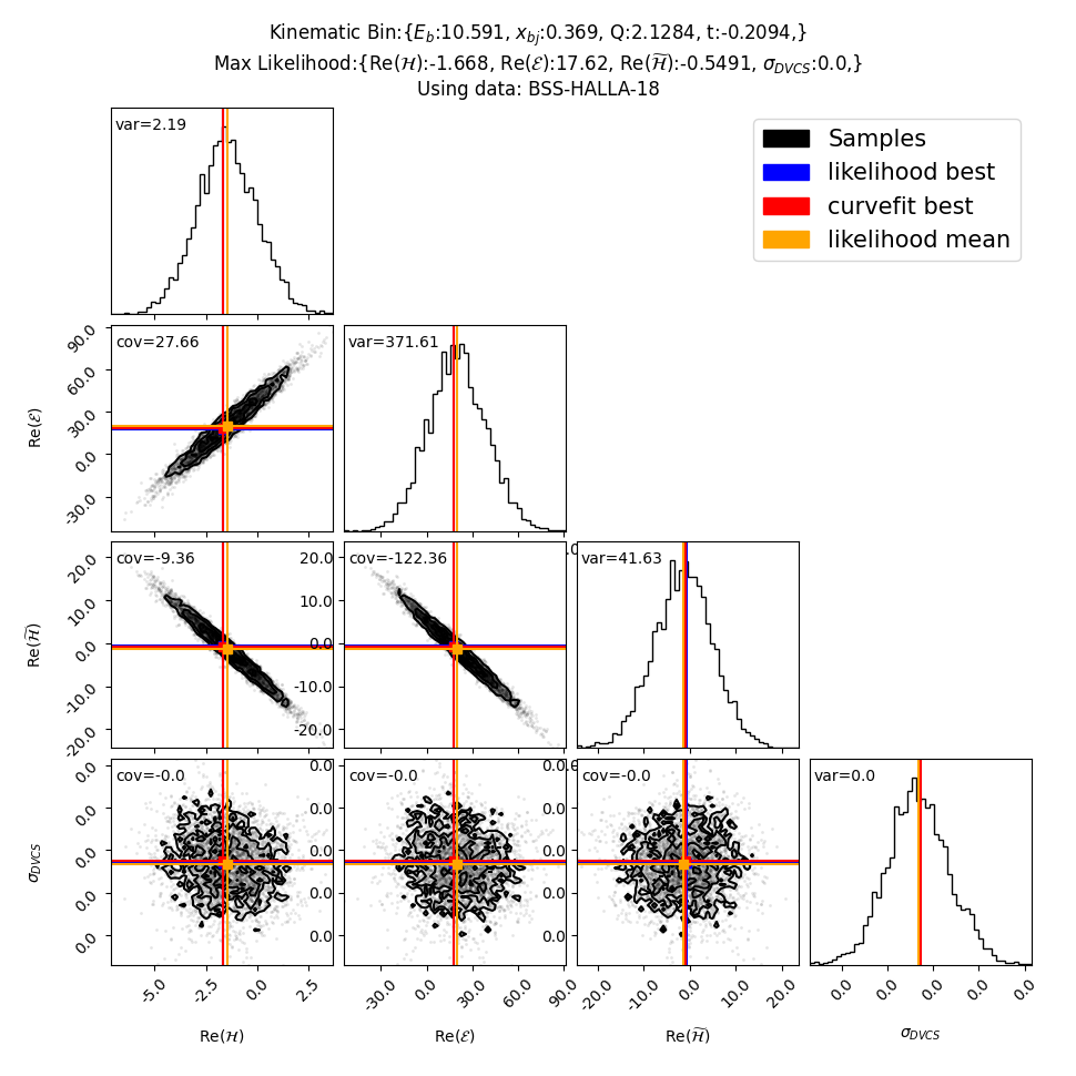
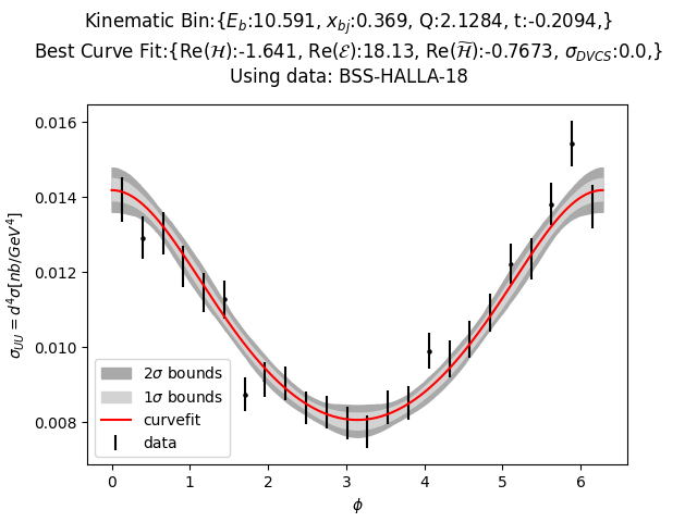
Figure 5: Canonical Result. Left: Corner plot using corner.py Foreman-Mackey (2016) of three CFFs: $\Re e{\cal H}$, $\Re e{\cal E}$, $\Re e\widetilde{{\cal H}}$, as well as an extra parameter, $\sigma_{DVCS}$, treated as a fourth free parameter independent of the angle $\phi$. Right: Error bands are generated by drawing 1000 curves, and then at each $\phi$ value finding the cross section values which is located above/below 95% of the curves. The Red curve corresponds to the best fit CFF parameters using a global optimizer geared towards general least squares in python scipy. The Blue curve corresponds to the MCMC sample of CFF parameters which has the largest likelihood. Red and Blue curves have nearly identical CFF parameters.

To improve on this situation we performed a study of the dependence on the experimental data distributions, focusing, in particular, on the following questions:

1. if outliers can be identified, and subtracted, does this lead to an improved analysis?

2. are the data too noisy?

Model	$\mu_{H}$	$\mu_{E}$	$\mu_{Ht}$	$\Sigma_{H,H}$	$\Sigma_{E,E}$	$\Sigma_{Ht,Ht}$	$\Sigma_{H,E}$	$\Sigma_{E,Ht}$	$\Sigma_{H,Ht}$
Canonical	-1.69	17.6	-0.549	2.19	371	41.6	27.7	122	9.36
No outls.	-1.251	25.18	-4.146	2.28	367	43.2	27.9	123	9.67

Table 2: Table of single kinematic bin results. CFF results for the canonical fit. The CFFs shown are the mean value as well as their covariances. Results for different methods of outlier testing are shown.

The outcome of point 1) is reported in Figure 6 where on the lhs we show a corner plot that correspond to the data once the outliers are removed as in the graph shown on the figure’s rhs. Results of the central values of the CFFs and details of the error analysis are presented in Table 2 (second row).

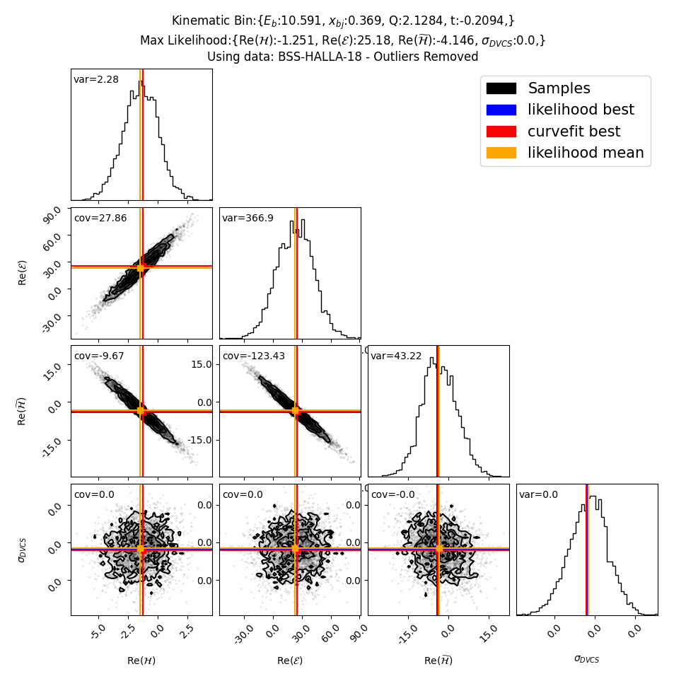
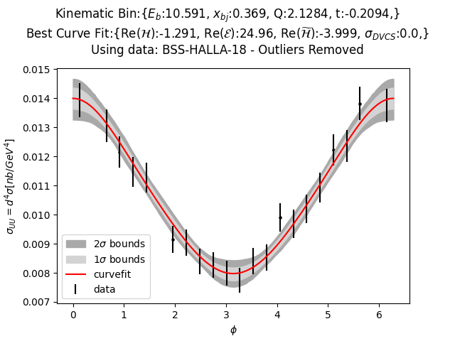
Figure 6: Left: Corner plot resulting from the analysis where experimental data which are considered to be outliers are removed from the analysis. The latter are shown plotted vs. $\phi$; Right: Graph of DVCS cross section with outlier points removed. On the right plot error bands are generated by drawing 1000 curves, and then at each $\phi$ value finding the cross section values which is located above/below 68% or 95% of the curves. The Red curve corresponds to the best fit CFF parameters using a global optimizer geared towards general least squares in python scipy. The Blue curve corresponds to the MCMC sample of CFF parameters which has the largest likelihood. Red and Blue curves have nearly identical CFF parameters.

We notice that, while the accuracy of the parameters prediction seems to improve, leading to a softening of the strong correlation found in the initial analysis, the treatment of outliers considered here is not founded on an objective methodology. Outliers were chosen expected from the symmetry of the $\phi$ dependence and removed points were those that lay at least $2\sigma$ away from the curve. Nevertheless, the present experimental data does show points that are substantially farther from the expected symmetric behavior in $\phi$, granting the necessity of future development of a dedicated procedure on how to systematically and properly treat this issue quantitatively as more data sets become available.

We also performed the fit including only half of the data points for each $\phi$ spectrum, that is choosing either the points with $\phi\equiv[0,\pi]$ or $\phi\equiv[\pi,2\pi]$. The reason to do this is that, while reducing the number of available data points, this method provides yet another way to overcome the potentially problematic question of the lack of symmetry in $\phi$ of experimental data. Nevertheless, the results show very little variation from the original plots in Fig.(5), indicating that the deviations of the data from a perfectly symmetric distribution around $\phi=\pi$, do not affect the outcome.

IV.2 Difference

Next, we show results of a likelihood analysis which assesses the difference of two cross section measurements at different angles (Figure 7). The difference method uses a multivariate gaussian with a covariance matrix.

In this case, the DVCS cross section drops out of the analysis. The numerical values of the extracted parameters are reported in Table 3.

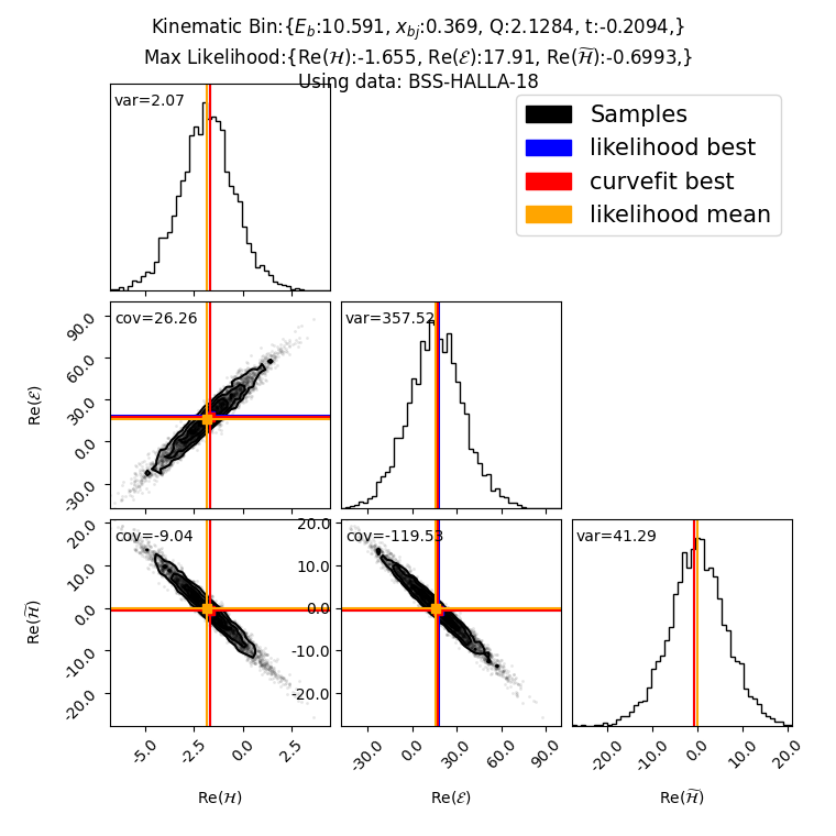
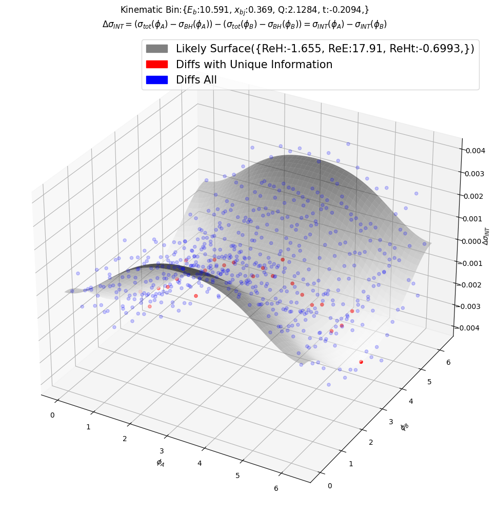
Figure 7: Left: Corner plot using the corner.py library of 3 CFFs: $\Re e{\cal H}$, $\Re e{\cal E}$, $\Re e\widetilde{\cal{H}}$. The cross section difference likelihood is defined as in equation 16. The cross section difference likelihood is explored using the emcee MCMC algorithm Foreman-Mackey et al. (2013). Right: Surface plot of the maximum likelihood parameters against the difference of two cross sections at all possible angles. The Blue points are all possible cross section differences. The Red points are those used in performing the fit to obtain the grey surface. The information contained in all blue points is fully contained in the red points only.

$E$ (GeV)	$x_{Bj}$	$Q$ (GeV)	$t$ (GeV2)	$\mu_{H}$	$\mu_{E}$	$\mu_{Ht}$	$\Sigma_{H,H}$	$\Sigma_{E,E}$	$\Sigma_{Ht,Ht}$	$\Sigma_{H,E}$	$\Sigma_{H,Ht}$	$\Sigma_{E,Ht}$
4.487	0.483	1.646	-0.391	-4.493	0.173	5.454	9.726	35.722	55.462	18.007	-22.596	-42.475
4.487	0.483	1.646	-0.348	-12.779	-18.875	30.908	52.929	242.426	293.722	112.673	-123.436	-263.223
4.487	0.484	1.646	-0.435	-0.927	8.229	-2.092	7.424	20.815	42.313	11.453	-17.004	-27.473
4.487	0.485	1.646	-0.480	-6.142	5.385	6.293	11.723	17.263	47.518	11.581	-22.028	-25.109
4.487	0.485	1.649	-0.540	-19.579	6.592	26.070	17.562	8.300	37.734	3.584	-22.864	-10.353
7.383	0.363	1.780	-0.297	-0.776	0.393	0.186	0.197	16.700	3.797	1.284	-0.743	-7.005
7.383	0.363	1.780	-0.211	-1.867	-9.750	6.738	0.890	94.007	14.793	8.699	-3.503	-36.194
7.383	0.364	1.783	-0.586	-6.223	9.507	9.146	2.535	14.261	6.156	-2.366	-2.234	-3.500
7.383	0.365	1.783	-0.471	-4.490	2.274	4.029	0.569	12.488	4.515	0.540	-0.969	-5.578
7.383	0.365	1.783	-0.385	-2.467	3.188	2.867	0.200	11.356	3.134	0.533	-0.544	-4.787
8.521	0.367	1.910	-0.266	-3.154	4.729	4.138	0.256	27.333	5.037	2.154	-1.029	-10.802
8.521	0.367	1.910	-0.205	-0.324	24.985	-7.389	1.256	172.650	21.984	14.256	-5.124	-60.197
8.521	0.369	1.916	-0.330	-2.951	10.543	1.446	0.235	18.439	4.104	1.194	-0.774	-7.623
8.521	0.370	1.918	-0.480	-5.214	12.863	2.266	0.820	7.746	2.560	-0.098	-0.890	-2.846
8.521	0.370	1.918	-0.392	-2.918	14.490	0.311	0.430	14.241	3.698	0.826	-0.862	-5.817
8.521	0.610	2.366	-0.764	-0.987	-0.767	1.427	0.846	22.534	13.381	4.285	-3.302	-17.062
8.521	0.612	2.371	-0.904	-1.249	1.726	-0.867	0.193	3.512	3.172	0.742	-0.740	-3.106
8.521	0.615	2.375	-1.048	-1.181	6.689	-3.413	0.161	2.180	2.470	0.459	-0.552	-2.003
8.521	0.616	2.379	-1.373	-2.426	5.341	0.875	0.439	1.361	2.616	0.278	-0.737	-1.453
8.521	0.617	2.377	-1.190	-2.099	3.914	1.694	0.245	1.912	2.948	0.401	-0.671	-2.004
8.847	0.482	2.309	-0.385	4.663	16.563	-12.772	24.800	197.164	133.490	69.492	-57.109	-160.615
8.847	0.483	2.311	-0.446	-0.632	3.471	1.516	5.239	32.840	28.507	12.549	-11.947	-29.513
8.847	0.485	2.315	-0.508	-3.060	1.339	4.197	3.836	17.411	18.690	7.323	-8.084	-16.785
8.847	0.486	2.317	-0.570	-1.961	5.909	1.328	4.429	13.749	16.213	5.817	-7.862	-13.116
8.847	0.486	2.319	-0.655	-7.329	2.650	6.605	4.030	6.017	9.520	1.643	-5.323	-5.131
8.851	0.497	2.121	-0.410	-1.580	-3.137	1.537	0.718	349.240	51.819	15.153	-5.874	-132.602
8.851	0.501	2.128	-0.480	-2.234	2.023	0.865	0.228	49.731	10.236	2.598	-1.262	-21.521
8.851	0.504	2.135	-0.548	-2.984	8.501	1.573	0.259	26.770	6.979	1.731	-1.002	-12.708
8.851	0.506	2.138	-0.614	-3.908	9.782	4.305	0.337	22.680	7.206	1.330	-0.973	-11.665
8.851	0.508	2.142	-0.707	-3.673	18.717	-0.093	0.447	11.303	3.918	0.710	-0.740	-5.712
10.591	0.369	2.128	-0.209	-1.629	18.226	-0.828	1.988	317.897	36.895	24.257	-8.367	-106.116
10.591	0.370	2.133	-0.272	-2.133	29.686	-2.671	0.533	65.893	10.173	4.862	-2.112	-24.319
10.591	0.371	2.138	-0.483	-2.118	15.254	-1.618	1.191	20.746	4.516	-0.345	-1.264	-6.909
10.591	0.372	2.138	-0.336	-2.420	23.001	-3.923	0.393	38.624	6.906	2.251	-1.277	-14.776
10.591	0.373	2.140	-0.399	-2.882	6.871	0.556	0.621	34.084	6.696	1.344	-1.253	-12.933
10.591	0.608	2.905	-0.791	-2.117	0.404	1.683	15.910	3.673	37.487	7.533	-24.289	-11.525
10.591	0.609	2.907	-0.912	0.306	1.666	-1.912	2.970	0.446	6.897	0.993	-4.456	-1.530
10.591	0.611	2.912	-1.037	-0.089	2.729	-2.292	1.667	0.230	3.948	0.383	-2.491	-0.638
10.591	0.613	2.915	-1.163	0.478	3.517	-3.356	2.054	0.257	3.943	0.033	-2.674	-0.262
10.591	0.613	2.917	-1.328	-1.952	3.271	-0.367	2.374	0.484	3.158	-0.641	-2.511	0.392
10.992	0.494	2.653	-0.432	2.230	9.396	-3.736	14.674	50.633	57.667	26.937	-28.887	-53.245
10.992	0.498	2.663	-0.526	2.113	7.448	-4.848	4.001	9.605	14.664	5.644	-7.418	-11.202
10.992	0.498	2.665	-0.856	-8.611	8.704	5.592	5.203	4.212	5.014	-2.748	-4.394	0.682
10.992	0.499	2.666	-0.698	-0.050	6.829	-3.897	5.231	5.042	9.956	0.949	-6.359	-4.004
10.992	0.499	2.668	-0.613	-2.138	4.206	2.019	3.824	5.002	10.463	3.070	-5.913	-6.159

Table 3: Table of kinematic bins, and CFF results for the “difference” fit. The CFF results shown are the mean value as well as non-redundant covariances between the the CFFs. Means and covariances are calculated using samples generated with Markov Chain Monte Carlo (MCMC) upon the difference likelihood, Eq.(16).

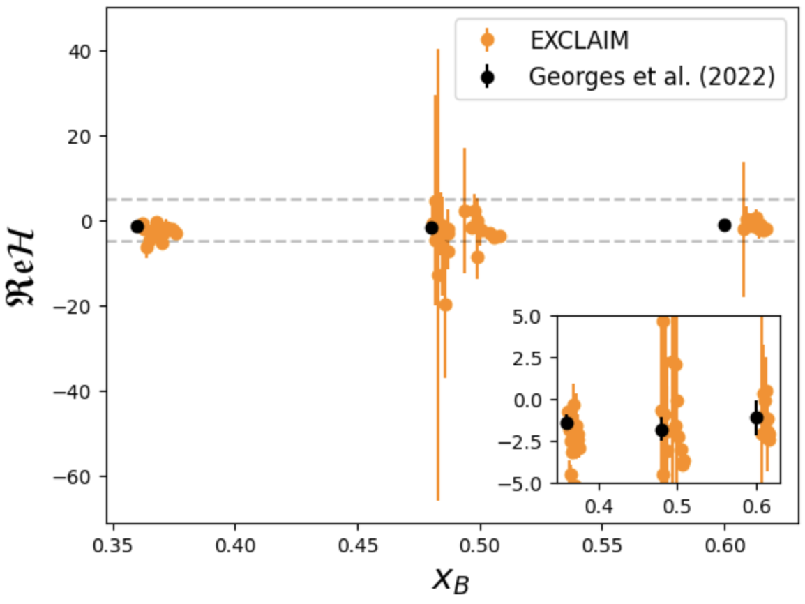
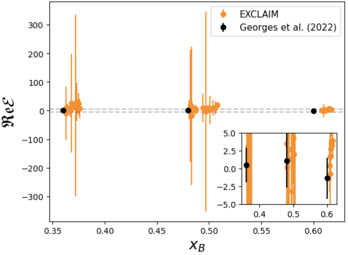
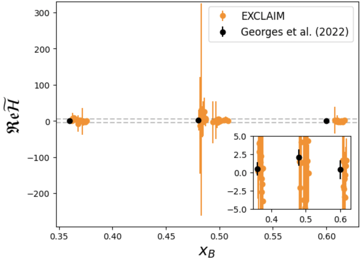
Figure 8: Visualization of the Compton form factors presented in Table 3 for the three kinematic bins in $x_{B}$ reported in Georges et al. (2022) compared to the CFFs extracted in Georges et al. (2022). The EXCLAIM error values correspond to the covariances $\Sigma_{H,H}$, $\Sigma_{E,E}$, and $\Sigma_{\widetilde{H},\widetilde{H}}$.

IV.3 Correlations study

Our numerical analysis shows that, based on the set of data examined, we can extract quantitatively only three CFFs, $\Re e{\cal H}$, $\Re e{\cal E}$, and $\Re e\widetilde{{\cal H}}$. Furthermore, we always have covariant results obtained through both likelihood methods. Here we investigate possible causes for the covariance, and we suggest ways around it. Throughout this work, we singled out various sources that could generate the strong correlations seen in the analysis, one by one showing their impact. We ruled out various possibilities while singling out which could be the most probable cause of correlation effects. Having ruled out aspects of the experimental data in the previous sections, the characteristic correlation structure that emerges from our analysis could be due to:

1. cross section formulation and its specific $t$ dependence

2. perturbations due to non-leading terms/twist-three contributions to the cross section

3. asymmetry in size of the kinematic coefficients

IV.3.1 Kinematic dependence of cross section

One possible cause for covariant results is the form of the interference term of the cross section formula itself in the specific regime of interest. From Eq.(7), one can see that $\Re e{\cal H}$ and $\Re e{\cal E}$ cannot be simultaneously constrained, i.e. they are degenerate, in the regime where $F_{1}(t)\approx\tau F_{2}(t)$. The ratio $F_{1}(t)\approx\tau F_{2}(t)$ is shown in Figure 9 where one can clearly see that this value is approached for at larger values of $-t$ than the range of present experimental data (their values of $-t$ do not exceed 2 GeV²). Therefore this source of correlation can be safely ruled out.

Figure 9: Ratio $\tau F_{2}/F_{1}$. One can see that this quantity is not close to 1 for the present range of data ($-t<2$ GeV²) and thus it is unlikely to be the cause of the degeneracy of our CFF parameter extraction.

IV.3.2 Beyond the leading order

Finally, we investigated the role of non leading order corrections, specifically whether omitting twist-three terms in the QCD formulation leads to inconsistent results. The reduced cross section given by,

$$\sigma_{\text{Reduced}}\equiv\dfrac{Q^{2}\left(\sigma_{TOT}-\sigma_{BH}\right)}{\Gamma}$$ (18)

is expected to be mildly $Q^{2}$ dependent in a QCD factorized framework, displaying logarithmic scaling violations at finite $Q^{2}$. Nevertheless, it has been known for long that a tension exists between the leading – logarithmic – and subleading, $Q^{2}$ inverse powers dominated, twist contributions in QCD (we refer the reader to Pennington (1983); Brock et al. (1995) for earlier reviews on the subject, to Yang and Bodek (2000) for an experimental study, and to Batelaan et al. (2023) for a recent lattice QCD exploration). Higher twist effects are expected to be present in the large $x_{Bj}$ region where Jefferson Lab data are concentrated, therefore many analyses of DVES data have been concerned with their determination Defurne et al. (2015, 2017); Georges (2018); Georges et al. (2022).

In Fig. 10, we plot the reduced cross section using data reported by the Jefferson Lab Hall A collaboration Georges (2018) with respect to $Q^{2}$.

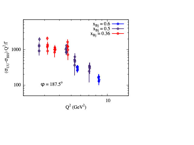
Figure 10: Example of reduced (dimensionless) cross section data from the Jefferson Lab Hall A collaboration Georges (2018) as a function of $Q^{2}$ for different $x_{Bj}$ in the kinematic bin $\phi=187.5^{\rm o}$. The $x_{Bj}$ values are indicated in color. For each $x_{Bj}$ and $Q^{2}$ bin, several values of $t$ are available, yielding the spread of points in the figure. Similar trends are found for the other measured values of $\phi$.

Each $x_{Bj}$ bin value contains data at different values $E$ and $t$, for a given $\phi$ value, although a similar behavior is shown for the other kinematic bins. The spread in the reduced cross section values for each chosen kinematics is due to the $t$ dependence of the data. From the trend of the data in $Q^{2}$, we deduce that the effect of $Q^{2}$ dependence other than logarithmic, such as e.g. the one given by higher twist terms cannot be ruled out.

By performing a likelihood analysis along the lines of the leading order one, we are faced with the situation where for the next non leading order contribution – which is expected to be of twist three Kriesten et al. (2020) – there are eight new complex CFFs, from the eight twist-three GPDs, which translate, in general, into sixteen unknowns Kriesten et al. (2020); Kriesten and Liuti (2022); Meissner et al. (2009).

In this case, the DVCS and DVCS-BH interference contributions to the cross section read,

$$\sigma_{DVCS} = \frac{\Gamma}{Q^{2}(1-\epsilon)}\left\{F_{DVCS}^{tw2}+\sqrt{\frac{t_{0}-t}{Q^{2}}}\sqrt{\epsilon(1+\epsilon)}\cos\phi\,F_{DVCS}^{tw3}\right\}$$ (19)

$$\sigma_{\cal I} = \frac{\Gamma}{Q^{2}}\left\{F_{\cal I}^{tw2}+\sqrt{\frac{t_{0}-t}{Q^{2}}}F_{\cal I}^{tw3}\right\}$$ (20)

where $F_{DVCS}^{tw2}$ and $F_{\cal I}^{tw2}$, the unpolarized electron-proton twist two contributions, can be read off Eqs.(5) and (7).

The unpolarized electron-proton twist three contributions read,

$$F_{DVCS}^{tw3} = -2\,(1-\xi^{2})\,\Re{\rm e}\Bigg{\{}\left(2\widetilde{\cal H}_{2T}+{\cal E}_{2T}+2\widetilde{\cal H}^{\prime}_{2T}+{\cal E}^{\prime}_{2T}\right)^{*}\Big{(}{\cal H}-\frac{\xi^{2}}{1-\xi^{2}}\mathcal{E}\Big{)}$$ (21)

$$+ \Big{(}\mathcal{H}_{2T}+\tau\widetilde{\mathcal{H}}_{2T}+\mathcal{H}_{2T}^{\prime}+\tau\widetilde{\mathcal{H}}_{2T}^{\prime}\Big{)}^{*}\Big{(}\mathcal{E}-\xi\widetilde{\mathcal{E}}\Big{)}$$

$$- 2\xi\,\left(\widetilde{\cal E}_{2T}+\widetilde{\cal E}^{\prime}_{2T}\right)^{*}\Big{(}\widetilde{\cal H}-\frac{\xi^{2}}{1-\xi^{2}}\widetilde{\mathcal{E}}\Big{)}+\frac{\xi}{1-\xi^{2}}\Big{(}\widetilde{\mathcal{E}}_{2T}-\xi\mathcal{E}_{2T}+\widetilde{\mathcal{E}}_{2T}^{\prime}-\xi\mathcal{E}_{2T}^{\prime}\Big{)}^{*}\Big{(}\mathcal{E}-\xi\widetilde{\mathcal{E}}\Big{)}$$

$$+ \frac{\tau}{4}\Big{(}\mathcal{\widetilde{H}}_{2T}+\mathcal{\widetilde{H}}_{2T}^{\prime}\Big{)}^{*}\Big{(}\mathcal{E}+\xi\widetilde{\mathcal{E}}\Big{)}\Bigg{\}}$$

$$F_{\cal I}^{tw3} = A^{(3)}_{\cal I}\Re e\Bigg{\{}F_{1}\Big{(}(2\mathcal{\widetilde{H}}_{2T}+\mathcal{E}_{2T})-(2\widetilde{\mathcal{H}}^{\prime}_{2T}+\mathcal{E}_{2T}^{\prime})\Big{)}+F_{2}\Big{(}(\mathcal{H}_{2T}+\tau\mathcal{\widetilde{H}}_{2T})-(\mathcal{H}_{2T}^{\prime}+\tau\widetilde{\mathcal{H}}_{2T}^{\prime})\Big{)}\Bigg{\}}$$ (22)

$$+ B^{(3)}_{\cal I}(F_{1}+F_{2})\,\Re e\Big{\{}\widetilde{\mathcal{E}}_{2T}-\xi{\cal E}_{2T}-\xi(\widetilde{\mathcal{E}}_{2T}^{\prime}-\xi{\cal E}^{\prime}_{2T})+\xi{\cal E}_{2T}-\xi^{2}E^{\prime}_{2T}\Big{\}}$$

$$+ C^{(3)}_{\cal I}(F_{1}+F_{2})\,\Re e\Bigg{\{}2\xi(\mathcal{H}_{2T}-\mathcal{H}_{2T}^{\prime})-\tau\Big{(}\widetilde{\mathcal{E}}_{2T}-\xi\mathcal{E}_{2T}-(\,\widetilde{\mathcal{E}}_{2T}^{\prime}+\xi\mathcal{E}_{2T}^{\prime})\Big{)}\Bigg{\}}$$

In the unpolarized cross section we single out only three vector coupling GPDs, i.e. only an additional one at twist three, corresponding to the quark-proton polarizations, $UU,UT,UL$ described respectively, by the combinations,

• $2\widetilde{H}_{2T}+E_{2T}$, the twist three polarization configuration analogous to the twist two $H$, unpolarized quark in unpolarized proton, $UU$;

• $H_{2T}+\,\tau\widetilde{H}_{2T}$, twist three polarization configuration analogous to the twist two $E$, unpolarized quark in transversely polarized proton, $UT$;

• $\widetilde{E}_{2T}-\xi E_{2T}$, corresponding to an unpolarized quark in longitudinally polarized proton, $UL$, that has no analogous at twist two due to parity conservation (see discussion in Refs.Courtoy et al. (2014); Rajan et al. (2016, 2018)). This term is important to the overall picture because it describes the orbital component of angular momentum Kiptily and Polyakov (2004); Hatta (2012); Rajan et al. (2018).

Similarly, we have three terms with axial-vector couplings described by the GPDs and CFFs with a $\prime$ superscript,

• $2\widetilde{H}^{\prime}_{2T}+E^{\prime}_{2T}$, the twist three polarization configuration analogous to $\widetilde{H}$, unpolarized quark in unpolarized proton, $LL$;

• $H^{\prime}_{2T}+\,\tau\widetilde{H}^{\prime}_{2T}$, twist three polarization configuration analogous to $E$, unpolarized quark in transversely polarized proton, $LT$;

• $\widetilde{E}^{\prime}_{2T}-\xi E^{\prime}_{2T}$, corresponding to a longitudinally quark in an unpolarized proton, $LU$, that also has no analogous at twist two due to parity conservation (see discussion in Refs.Courtoy et al. (2014); Rajan et al. (2016, 2018)). This term describes the quark spin orbit contribution Kiptily and Polyakov (2004); Hatta (2012); Rajan et al. (2018).

(see Kriesten and Liuti (2022), for a more extensive discussion of the physical meaning of these terms).

The coefficients, $A^{(3)}_{\cal I}$, $B^{(3)}_{\cal I}$, $C^{(3)}_{\cal I}$ are written in terms of four-vector products involving all relevant kinematics variables. Similarly to the twist-two case, they can be expressed in terms of the set of variables ($Q^{2}$, $x_{Bj}$, $t$, $\phi$). Their specific expressions are rather lengthy and are given explicitly in Ref.Kriesten et al. (2020). For the present analysis it is important to point out that the twist-three DVCS cross section, Eq.(19), depends on $\cos\phi$, thus complicating the outcome of a possible analysis in the canonical framework. Results are plotted in Figure 11.

Our analysis points out that twist three CFFs, although they are likely to be an important component, contain degeneracy and require careful analysis and approach to perform an MCMC correctly. We have written software with the fully twist-3, used the canonical likelihood, and attempted to constrain the CFFs using MCMC against the data ignoring any possible degeneracy to produce Figure 11. We note however that we are not highly confident in the twist-3 results shown because in general MCMC methods do not behave well under degenerate conditions.

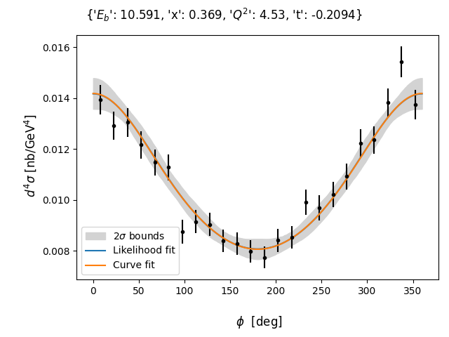
Figure 11: Left: Corner plot with twist-3 CFFs included. CFF parameters bounded by hyperbox $[-100,100]$ while $F_{UU,T}$ and $F^{\cos(\phi)}_{UU}$ bounded between $[-10000,10000]$. 5000 samples are included in this graph. The best fit likelihood occurs at: [ 4.57, -73.52, -8.40, -8.42, 28.13, 60.34, 20.04, 8.17, -623.13]. Right: Likelihood fit with twist-3 CFFs included, corresponding to the lhs panel. Error bands are generated by drawing 1000 curves on this plot and finding the cross section values, for each $\phi$ value, located above/below 95% of the curves. The orange curve corresponds to the best fit CFF parameters which draw a curve through the data. The blue curve (which appears superimposed to the orange one) corresponds to the MCMC sample of CFF parameters which has the largest likelihood.

V Conclusions and Outlook

We presented a new paradigm for the analysis of deeply virtual exclusive photoproduction off a proton target, $ep\rightarrow e^{\prime}p^{\prime}\gamma^{\prime}$, using a model for likelihood-based inference in high dimensional data settings.

The deeply virtual Compton scattering contribution to the cross section, where the photon is produced at the proton vertex, is described in terms of Compton form factors which, in a QCD factorized scenario can be written as convolutions of GPDs, which are believed to contain important information on the proton 3D structure. The extraction of Compton form factors from data represents, therefore, the first step in obtaining the latter from data.

We obtained joint (statistically) covariant results for Compton form factors using a twist-two cross section model for the unpolarized process for which the largest amount of data with all the kinematic dependences are available from corresponding datasets from Jefferson Lab. Our analysis provides a method which derives a joint likelihood of the latter, for each observed combination of the kinematic variables defining the reaction, $[E_{b},x_{B},t,Q^{2}]$, and varying azimuthal angles $\phi$. Based on the observation that the unpolarized twist-two cross section likelihood fully constrains only three of the Compton form factors, the derived difference-model likelihoods were explored using Markov chain Monte Carlo (MCMC) methods. Error bars, covariances and associated joint $n-\sigma$ confidence contours were evaluated. Our main results for the twist-two cross section are presented in a 45 rows table (Table 3), one row for each unique kinematic bin from our available unpolarized DVCS dataset Kumerički (2022) Georges (2018). Results are also shown using corner plots to highlight the impact of the covariances in the analysis.

What can be done to reduce the size of the $n-\sigma$ contours? Using a more “well behaved” set of data does not substantially help. At the same time we see that higher twists are important. This casts doubts on the validity of a QCD factorized description approach Collins and Freund (1999) for the present kinematic setting, and motivates both further investigations, e.g. at EIC kinematics which guarantees a large $Q^{2}$ span. Previous HERA data Adloff et al. (2001) as precursors to the EIC, could also provide additional information, as it would extending the analysis to include constraints from other types of data (considering other polarization configurations, e.g. longitudinally and transversely polarized targets and recoil target polarization) for which at present, only simulations are made available.

One error reducing method we plan to explore is known as “outlier pruning” Hogg et al. (2010). The procedure involves designing an analysis that allows for each data point considered to have an effective weighting based on the probability of the point being an outlier. Then these outlier probabilities are marginalized in the final likelihood analysis in the MCMC step. The method either introduces many additional parameters which must be marginalized over, or requires clever math methods which roll the additional parameters into few parameters. We plan to attempt a statistically sound outlier pruning in our next paper.

The impact of the twist-three corrections to the analysis was explored but the current status of the analysis is incomplete: while we included the calculations of the twist-three corrections which introduce sixteen additional Compton form factors, and calculated an introductory twist-three canonical likelihood, we note that a proper likelihood analysis treatment in this case requires careful assessment of degeneracy in the Compton form factors. Thus we relegate a careful twist-three parameter degeneracy investigation to future work. Once the basic physics framework (QCD factorization) is established, we will be in a position to constrain the CFFs using other sets of data to including parton distributions from deep inelastic inclusive scattering and opening to lattice QCD.

In summary, our present analysis lays out the statistics foundation of our new framework which leverages state of the art ML algorithms to carry out efficiently Bayesian inference in high-dimensional settings. Companion manuscripts to the present one, addressing the connection with ML can be found in Refs.Almaeen et al. (2024); Hossen et al. (2024).

Previous analyses Georges et al. (2022) do not agree with our results. The analyses of deeply virtual exclusive experiments conducted so far do not provide a publicly available, common set of benchmarks of their statistical approaches, and thus we are not in a position to attempt to reproduce existing results for comparison. Nevertheless, Fig.8 shows a comparison of our analysis with published results. From our analysis we conclude that in order to validate a QCD factorized scenario from which the observables for the 3D structure of the proton could be extracted, it is important to perform measurements for different target polarizations, both longitudinal and transverse, as well as at the lowest $t/Q^{2}$ ratio and widest $Q^{2}$ range possible.

Appendix A BH coefficients

The BH coefficients in Eq.(2) read,

$$A_{BH}= \frac{{8}\,M^{2}}{t(k\,q^{\prime})(k^{\prime}\,q^{\prime})}\Bigg{[}4\tau\Big{(}(k\,P)^{2}+(k^{\prime}\,P)^{2}\Big{)}-(\tau+1)\Big{(}(k\,\Delta)^{2}+(k^{\prime}\,\Delta)^{2}\Big{)}\Bigg{]}$$ (23)

$$B_{BH}= \frac{{16}\,M^{2}}{t(k\,q^{\prime})(k^{\prime}\,q^{\prime})}\Big{[}(k\,\Delta)^{2}+(k^{\prime}\,\Delta)^{2}\Big{]}\,,$$ (24)

where $P=(p+p^{\prime})/2$, $\tau=-t/4M^{2}$. The four vector products, $(ab)=a_{o}b_{o}-{\bf a}\cdot{\bf b}$, can be evaluated by for either the fixed target or collider settings.

Appendix B Interference coefficients

The BH-DVCS interference cross section coefficients in Eq.(7) read,

$$A_{UU}^{\cal I} = -8\frac{D_{+}}{t}\Big{[}(k^{\prime}P)\Big{(}2k_{T}^{2}-k_{T}\cdot q_{T}^{\prime}-2(kq^{\prime})\Big{)}+(kP)\Big{(}2k^{\prime}_{T}\cdot k_{T}+k^{\prime}_{T}\cdot q^{\prime}_{T}+2(k^{\prime}q^{\prime})\Big{)}-(k_{T}\cdot P_{T})\Big{(}2(kk^{\prime})+(k^{\prime}q^{\prime})\Big{)}$$ (25)

$$+ (k_{T}^{\prime}\cdot P_{T})(kq^{\prime})\Big{]}\cos\phi-8D_{-}\Big{[}(Pq^{\prime})\Big{(}2k_{T}\cdot k^{\prime}_{T}+2(kk^{\prime})\Big{)}-(k_{T}\cdot P_{T})(k^{\prime}q^{\prime})-(k_{T}^{\prime}\cdot P_{T})(kq^{\prime})$$

$$+ (P_{T}\cdot q_{T}^{\prime})(kk^{\prime})\Big{]}\cos\phi$$

$$B_{UU}^{\cal I} = -4\xi\frac{D_{+}}{t}\Big{[}(k^{\prime}\Delta)\Big{(}2k_{T}^{2}-k_{T}\cdot q_{T}^{\prime}-2(kq^{\prime})\Big{)}+(k\Delta)\Big{(}2k^{\prime}_{T}\cdot k_{T}+k^{\prime}_{T}\cdot q^{\prime}_{T}+2(k^{\prime}q^{\prime})\Big{)}-(k_{T}\cdot\Delta_{T})\Big{(}2(kk^{\prime})+(k^{\prime}q^{\prime})\Big{)}$$ (26)

$$+ (k_{T}^{\prime}\cdot\Delta_{T})(kq^{\prime})\Big{]}\cos\phi-4\xi D_{-}\Big{[}(\Delta q^{\prime})\Big{(}2k_{T}\cdot k^{\prime}_{T}+2(kk^{\prime})\Big{)}-(k_{T}\cdot\Delta_{T})(k^{\prime}q^{\prime})-(k_{T}^{\prime}\cdot\Delta_{T})(kq^{\prime})$$

$$+ (q_{T}^{\prime}\cdot\Delta_{T})(kk^{\prime})\Big{]}\cos\phi$$

$$C_{UU}^{\cal I} = 4\frac{D_{+}}{tP^{+}}\Big{[}-(k_{T}\cdot P_{T})(q^{\prime}_{T}\cdot\Delta_{T})k^{\prime+}+(k_{T}\cdot\Delta_{T})(P_{T}\cdot q^{\prime}_{T})k^{\prime+}+(k^{\prime}_{T}\cdot P_{T})(q^{\prime}_{T}\cdot\Delta_{T})k^{+}$$ (27)

$$- (k^{\prime}_{T}\cdot\Delta_{T})(P_{T}\cdot q^{\prime}_{T})k^{+}-2(kk^{\prime})(k^{\prime}_{T}\cdot P_{T})\Delta^{+}-(kq^{\prime})(k^{\prime}_{T}\cdot P_{T})\Delta^{+}$$

$$+ (k^{\prime}q^{\prime})(k_{T}\cdot P_{T})\Delta^{+}+2(kk^{\prime})(k^{\prime}_{T}\cdot\Delta_{T})P^{+}+(kq^{\prime})(k^{\prime}_{T}\cdot\Delta_{T})P^{+}-(k^{\prime}q^{\prime})(k_{T}\cdot\Delta_{T})P^{+}\Big{]}\cos\phi$$

$$+ 4\frac{D_{-}}{tP^{+}}\Big{[}(k^{\prime}q^{\prime})(k_{T}\cdot P_{T})\Delta^{+}-(kk^{\prime})(q^{\prime}_{T}\cdot P_{T})\Delta^{+}+(kq^{\prime})(k^{\prime}_{T}\cdot P_{T})\Delta^{+}$$

$$- (k^{\prime}q^{\prime})(k_{T}\cdot\Delta_{T})P^{+}+(kk^{\prime})(q^{\prime}_{T}\cdot\Delta_{T})P^{+}-(kq^{\prime})(k^{\prime}_{T}\cdot\Delta_{T})P^{+}\Big{]}\cos\phi$$

where the “$T$” subscript refers to the transverse component of the given vectors with respect to the $ep$ direction; the $+$ superscript in the vectors, $v^{+}=(P^{+},\Delta^{+},k^{+},k^{\prime+})$, refers to the combination: $v^{+}=(v^{o}+v^{3})/\sqrt{2}$; $D_{+}$ and $D_{-}$ are defined as,

$$D_{+}=\frac{(kq^{\prime})-{(k^{\prime}q^{\prime}})}{2(k^{\prime}q^{\prime})(kq^{\prime})},\;\;\;\;\quad\quad\quad D_{-}=-\frac{(kq^{\prime})+{(k^{\prime}q^{\prime})}}{2(k^{\prime}q^{\prime})(kq^{\prime})}$$ (28)

The coefficients also receive a contribution from the electromagnetic gauge invariance preserving terms, which only mildly modifies the values of the coefficients. A complete definition of the coefficients up to twist three is given in Kriesten and Liuti (2022).

References

- Diehl (2001) M. Diehl, Eur.Phys.J. C19, 485 (2001), eprint hep-ph/0101335.
- Belitsky and Radyushkin (2005) A. Belitsky and A. Radyushkin, Phys.Rept. 418, 1 (2005), eprint hep-ph/0504030.
- Kumericki et al. (2016) K. Kumericki, S. Liuti, and H. Moutarde, Eur. Phys. J. A52, 157 (2016), eprint 1602.02763.
- Kriesten et al. (2020) B. Kriesten, S. Liuti, L. Calero-Diaz, D. Keller, A. Meyer, G. R. Goldstein, and J. Osvaldo Gonzalez-Hernandez, Phys. Rev. D 101, 054021 (2020), eprint 1903.05742.
- Kriesten et al. (2022a) B. Kriesten, S. Liuti, and A. Meyer, Phys. Lett. B 829, 137051 (2022a), eprint 2011.04484.
- Kriesten and Liuti (2022) B. Kriesten and S. Liuti, Phys. Rev. D 105, 016015 (2022), eprint 2004.08890.
- Punjabi et al. (2015) V. Punjabi, C. F. Perdrisat, M. K. Jones, E. J. Brash, and C. E. Carlson, Eur. Phys. J. A 51, 79 (2015), eprint 1503.01452.
- Kelly (2004) J. J. Kelly, Phys. Rev. C 70, 068202 (2004).
- Bradford et al. (2006) R. Bradford, A. Bodek, H. S. Budd, and J. Arrington, Nucl. Phys. B Proc. Suppl. 159, 127 (2006), eprint hep-ex/0602017.
- Brash et al. (2002) E. J. Brash, A. Kozlov, S. Li, and G. M. Huber, Phys. Rev. C 65, 051001 (2002), eprint hep-ex/0111038.
- Ji (1997a) X.-D. Ji, Phys. Rev. D 55, 7114 (1997a), eprint hep-ph/9609381.
- Radyushkin (1997) A. V. Radyushkin, Phys. Rev. D56, 5524 (1997), eprint hep-ph/9704207.
- Müller et al. (1994) D. Müller, D. Robaschik, B. Geyer, F. M. Dittes, and J. Hořejši, Fortsch. Phys. 42, 101 (1994), eprint hep-ph/9812448.
- Diehl (2003) M. Diehl, Phys. Rept. 388, 41 (2003), eprint hep-ph/0307382.
- Diehl (2002) M. Diehl, Eur. Phys. J. C 25, 223 (2002), [Erratum: Eur.Phys.J.C 31, 277–278 (2003)], eprint hep-ph/0205208.
- Burkardt (2003) M. Burkardt, Int. J. Mod. Phys. A 18, 173 (2003), eprint hep-ph/0207047.
- Soper (1977) D. E. Soper, Phys. Rev. D15, 1141 (1977).
- Ji (1997b) X.-D. Ji, Phys. Rev. Lett. 78, 610 (1997b), eprint hep-ph/9603249.
- Polyakov (2003) M. Polyakov, Phys. Lett. B 555, 57 (2003), eprint hep-ph/0210165.
- Shanahan and Detmold (2019) P. E. Shanahan and W. Detmold, Phys. Rev. Lett. 122, 072003 (2019), eprint 1810.07589.
- Lorcé et al. (2021) C. Lorcé, A. Metz, B. Pasquini, and S. Rodini, JHEP 11, 121 (2021), eprint 2109.11785.
- Diehl and Sapeta (2005) M. Diehl and S. Sapeta, Eur. Phys. J. C41, 515 (2005), eprint hep-ph/0503023.
- Almaeen et al. (2022) M. Almaeen, J. Grigsby, J. Hoskins, B. Kriesten, Y. Li, H.-W. Lin, and S. Liuti (2022), eprint 2207.10766.
- Almaeen et al. (2024) M. Almaeen, T. Alghamdi, B. Kriesten, D. Adams, Y. Li, S. Liuti, and H.-W. Lin (2024), eprint 2405.05826.
- Sofiatti and Donnelly (2011) C. Sofiatti and T. W. Donnelly, Phys. Rev. C84, 014606 (2011), eprint 1104.2149.
- Goldstein et al. (2013) G. Goldstein, J. O. Gonzalez-Hernandez, and S. Liuti (2013), eprint 1311.0483.
- Kriesten et al. (2022b) B. Kriesten, P. Velie, E. Yeats, F. Y. Lopez, and S. Liuti, Phys. Rev. D 105, 056022 (2022b), eprint 2101.01826.
- Georges et al. (2022) F. Georges et al. (Jefferson Lab Hall A), Phys. Rev. Lett. 128, 252002 (2022), eprint 2201.03714.
- Georges (2018) F. Georges, Ph.D. thesis, Institut de Physique Nucléaire d’Orsay, France (2018).
- Belitsky et al. (2002) A. V. Belitsky, D. Mueller, and A. Kirchner, Nucl. Phys. B 629, 323 (2002), eprint hep-ph/0112108.
- Braun et al. (2014) V. M. Braun, A. N. Manashov, D. Müller, and B. M. Pirnay, Phys. Rev. D89, 074022 (2014), eprint 1401.7621.
- Belitsky and Mueller (2010) A. V. Belitsky and D. Mueller, Phys. Rev. D82, 074010 (2010), eprint 1005.5209.
- Kumerički (2022) K. Kumerički, Gepard BSS HALL A dataset (2022), URL https://github.com/kkumer/gepard/blob/master/src/gepard/datasets/ep2epgamma/BSS-HALLA-18.dat.
- Foreman-Mackey et al. (2013) D. Foreman-Mackey, D. W. Hogg, D. Lang, and J. Goodman, Publications of the Astronomical Society of the Pacific 125, 306–312 (2013), ISSN 1538-3873, URL http://dx.doi.org/10.1086/670067.
- Foreman-Mackey (2016) D. Foreman-Mackey, Journal of Open Source Software 1, 24 (2016), URL https://doi.org/10.21105/joss.00024.
- Pennington (1983) M. R. Pennington, Rept. Prog. Phys. 46, 393 (1983).
- Brock et al. (1995) R. Brock et al. (CTEQ), Rev. Mod. Phys. 67, 157 (1995).
- Yang and Bodek (2000) U.-K. Yang and A. Bodek, Eur. Phys. J. C 13, 241 (2000), eprint hep-ex/9908058.
- Batelaan et al. (2023) M. Batelaan et al. (QCDSF/UKQCD/CSSM, CSSM, UKQCD, QCDSF), Phys. Rev. D 107, 054503 (2023), eprint 2209.04141.
- Defurne et al. (2015) M. Defurne et al. (Jefferson Lab Hall A), Phys. Rev. C92, 055202 (2015), eprint 1504.05453.
- Defurne et al. (2017) M. Defurne et al., Nature Commun. 8, 1408 (2017), eprint 1703.09442.
- Meissner et al. (2009) S. Meissner, A. Metz, and M. Schlegel, JHEP 0908, 056 (2009), eprint 0906.5323.
- Courtoy et al. (2014) A. Courtoy, G. R. Goldstein, J. O. Gonzalez-Hernandez, S. Liuti, and A. Rajan, Phys. Lett. B731, 141 (2014), eprint 1310.5157.
- Rajan et al. (2016) A. Rajan, A. Courtoy, M. Engelhardt, and S. Liuti, Phys. Rev. D 94, 034041 (2016), eprint 1601.06117.
- Rajan et al. (2018) A. Rajan, M. Engelhardt, and S. Liuti, Phys. Rev. D98, 074022 (2018), eprint 1709.05770.
- Kiptily and Polyakov (2004) D. Kiptily and M. Polyakov, Eur. Phys. J. C37, 105 (2004), eprint hep-ph/0212372.
- Hatta (2012) Y. Hatta, Phys. Lett. B708, 186 (2012), eprint 1111.3547.
- Collins and Freund (1999) J. C. Collins and A. Freund, Phys. Rev. D59, 074009 (1999), eprint hep-ph/9801262.
- Adloff et al. (2001) C. Adloff et al. (H1), Phys. Lett. B 517, 47 (2001), eprint hep-ex/0107005.
- Hogg et al. (2010) D. W. Hogg, J. Bovy, and D. Lang (2010), eprint 1008.4686.
- Hossen et al. (2024) F. Hossen et al. (2024), eprint 2408.11681.