Polarization position angle standard stars: a reassessment of and its variability for seventeen stars based on a decade of observations
Abstract
Observations of polarization position angle () standards made from 2014 to 2023 with the High Precision Polarimetric Instrument (HIPPI) and other HIPPI-class polarimeters in both hemispheres are used to investigate their variability. Multi-band data were first used to thoroughly recalibrate the instrument performance by bench-marking against carefully selected literature data. A novel Co-ordinate Difference Matrix (CDM) approach – which combines pairs of points – was then used to amalgamate monochromatic ( band) observations from many observing runs and re-determine for 17 standard stars. The CDM algorithm was then integrated into a fitting routine and used to establish the impact of stellar variability on the measured position angle scatter. The approach yields variability detections for stars on long time scales that appear stable over short runs. The best position angle standards are Car, Sco, HD 154445, HD 161056 and Sco which are stable to 0.123∘. Position angle variability of 0.27–0.82∘, significant at the 3- level, is found for 5 standards, including the Luminous Blue Variable HD 160529 and all but one of the other B/A-type supergiants (HD 80558, HD 111613, HD 183143 and 55 Cyg), most of which also appear likely to be variable in polarization magnitude () – there is no preferred orientation for the polarization in these objects, which are all classified as Cygni variables. Despite this we make six key recommendations for observers – relating to data acquisition, processing and reporting – that will allow them to use these standards to achieve 0.1∘ precision in the telescope position angle with similar instrumentation, and allow data sets to be combined more accurately.
keywords:
techniques: polarimetric; stars: supergiants; instrumentation: polarimeters1 Introduction
The 21st Century has seen the advent of broadband optical polarimeters capable of a precision of 10 parts-per-million or better. Their development was sparked by the hunt for exoplanet signatures (e.g. Hough et al., 2006; Wiktorowicz & Matthews, 2008; Piirola et al., 2014; Bailey et al., 2015) but instead lead to the discovery of new and predicted stellar polarigenic mechanisms, such as rapid rotation (Cotton et al., 2017; Bailey et al., 2020; Lewis et al., 2022; Howarth et al., 2023), binary photospheric reflection (Bailey et al., 2019; Cotton et al., 2020), linear polarization from global magnetic fields (Cotton et al., 2017; Cotton et al., 2019a), and non-radial pulsations (Cotton et al., 2022a). Precise maps of interstellar polarization close to the Sun are now possible (Cotton et al., 2016; Piirola et al., 2020), and inferences have been made about the nature of hot dust (Marshall et al., 2016), debris disks (Marshall et al., 2020, 2023), and even the heliosphere (Frisch et al., 2022). Higher precision studies of known phenomena are also revealing new details about such diverse topics as asteroids (Wiktorowicz & Nofi, 2015), gas entrained between binary stars (Berdyugin et al., 2018), the nature of the interstellar medium (Cotton et al., 2019b), and extreme variable stars (Bailey et al., 2024). Alongside this progress, the dream of detecting and characterising exoplanet atmospheres with polarimetry remains a live ambition (Bailey et al., 2021; Bott et al., 2022; Wiktorowicz, 2024). The development of new instruments continues at pace, both for medium to very large sized telescopes (Wiktorowicz & Nofi, 2015; Bailey et al., 2020; Piirola et al., 2021) and even amateur-sized telescopes (Bailey et al., 2017, 2023).
Despite the ground-breaking improvements in instrumental precision, polarimetric observations of objects at increasing distance are naturally affected by the interstellar polarization background. The detection of small polarization signals from distant objects is therefore critically dependant upon the accurate calibration of the polarization position angle – a craft that has not progressed at the same rate. We aim to address this issue here.
Linear polarization is defined either in terms of normalised Stokes parameters and (typically measured in per cent: , or parts-per-million, ppm: ), or as polarization magnitude,
| (1) |
and position angle,
| (2) |
measured North over East, relative to the North Celestial Pole (), i.e. in the Equatorial system. Polarimetric data is almost universally reported in either or both of these co-ordinate frames, but collected in an instrument frame, (, ), and then rotated according to,
| (3) |
and
| (4) |
where , usually called the telescope position angle, is the difference between the instrument reference axis and – which is readily accessible in astrometry but not polarimetry (Van De Kamp, 1967; Hsu & Breger, 1982)111Serkowski (1974b) summarises some alternative methods of finding , mostly involving polarizers carefully aligned to the horizon mounted external to the telescope, however Hsu & Breger (1982) infer the accuracy of these methods is not better than 1∘.. Instead polarimetrists often have to determine by reference to high polarization standard stars (Serkowski, 1974a, b). For this purpose, must be re-determined for every observing run (and whenever the equipment is disturbed) to reflect the current condition of the instrument and telescope. It is also a difficult task to perform with precision and accuracy, since the available calibration stars vary with observing location and season. Indeed, there can sometimes be no established standards in the sky bright enough for polarimetry on the smallest telescopes (e.g. the 10-inch telescopes used by Bailey et al., 2023 and Bailey et al., 2024).
Despite some standards apparently having determined to 0.2∘ accuracy (Hsu & Breger, 1982), the accuracy is usually considered to be only 1∘ (e.g. Wiktorowicz & Nofi, 2015; Bailey et al., 2020). With recent advances, 1∘ accuracy is not always good enough for the intended science (e.g. Cotton et al., 2020).
A good high polarization standard has two qualities: (i) it is non-variable (especially in ), and (ii) it has a high polarization relative to its brightness, since position angle uncertainty, , is related to polarization magnitude uncertainty, , (Serkowski, 1968; Hsu & Breger, 1982):
| (5) |
where is in degrees, and is a function of photon count when not limited by instrumentation or seeing.
Most ordinary stars have little intrinsic polarization. Instead the dominant polarizing mechanism is the interstellar medium (ISM) (Hiltner, 1949; Hall, 1949; Serkowski, 1968). As light travels from a star to the observer it interacts with oblate dust grains within the ISM aligned by large scale magnetic fields; these act like a wire grid polarizer. The interstellar polarization imparted is dependent on the uniformity of the ISM as well as the quantity of dust on the sight line – and hence, indirectly, on distance. Within about 100 pc of the Sun – i.e. within the Local Hot Bubble – interstellar polarization is imparted at a rate of about 0.2 to 2.0 ppm/pc (Bailey et al., 2010; Cotton et al., 2016, 2017), beyond that it is 20 ppm/pc (Behr, 1959).
The ISM is assumed to be unchanging on relevant astrophysical timescales, which leads to choosing standards that are relatively distant and bright. Typically, the best small telescope standards have polarizations of several percent, have , and have parallaxes 2-4 mas – these are necessarily some of the most extreme stars. The standards used today were mostly chosen in the 1960s and 1970s (Serkowski, 1968, 1974a, 1974b; Serkowski et al., 1975; Clarke, 2010), with much of the work establishing wavelength dependence and refining taking place from the 1970s to 1990s (Serkowski et al., 1975; Whittet & van Breda, 1980; Wilking et al., 1982; Whittet et al., 1992; Wolff et al., 1996; Martin et al., 1999). The most comprehensive modern re-examination of the wavelength dependence of interstellar polarization was provided by Bagnulo et al. (2017), but there are scant recent works222Wiktorowicz et al. (2023) and Bailey et al. (2023) make a cursory examination of a few standards as part of much broader works. And although Blinov et al. (2023) are conducting a monitoring campaign with the RoboPol instrument, this seems to include few, if any, bright standards. looking at the long term stability of the most important stars.
In the earlier literature there was an important debate about which standards might be variable. Hsu & Breger (1982), Dolan & Tapia (1986), Lupie & Nordsieck (1987), Bastien et al. (1988) and Clemens & Tapia (1990) all, often contrastingly, identified standards they considered to be variable. Of these, the most thorough analyses were performed by Hsu & Breger (1982) and Bastien et al. (1988). However, these works have all been criticised as not statistically rigorous by Naghizadeh-Khouei (1991), who pointed out that in most cases only partial data was presented and the data sets were small. The work of Bastien et al. (1988) was the most comprehensive, yet came in for particular criticism by Clarke & Naghizadeh-Khouei (1994), who in reanalysing their data were convinced of the variability of only one star out of the eleven claimed. There, the main objection was that the data were drawn from different sets without this being properly accounted for, and the reanalysis used only a subset of the observations. Some time later Bastien et al. (2007) revisited their work. They applied the Cumulative Distribution Function (CDF) test “in a very conservative manner” that was used and recommended by Clarke & Naghizadeh-Khouei (1994), concluding that 7 of the 11 stars they originally declared variable were, and that the other 4 “may be.” This does not seem a particularly satisfactory resolution. Consequently, a pall hangs over the question of which polarization standards are variable on long timescales, and the caution implied by Bastien et al. (1988)’s findings has gone substantially unheeded by observers.
Putting aside the controversy, more broadly there are three motivations that provoke further study of these stars:
-
1.
Interstellar polarization may not be constant on 50-yr timescales. On any given sight line there will be many different dust clouds, which are in motion with respect to our standard stars. Significant movement of the clouds would cause the observed value of to vary over time (Bastien et al., 1988; Clarke, 2010).
-
2.
Extreme stars are the most likely to have large intrinsic polarizations – intrinsic polarization is more common in stars of B-type and earlier333Furthermore, the more massive a star the more likely it is to have a close companion, which results in variable polarization, scattered either from material entrained betwixt the binary, or the photospheres of the components (see Cotton et al., 2020 for a historical overview of both mechanisms). and K-type and later (Cotton et al., 2016; Clarke, 2010), and in more luminous stars (Dyck & Jennings, 1971; Clarke, 2010; Lewis et al., 2022). Polarization variability could have a very long period, un-captured by prior shorter duration studies, or be episodic as in the case of Be stars (e.g Carciofi et al., 2007) or LBV stars (Gootkin et al., 2020). So, stars seemingly non-variable decades ago may not be so now.
-
3.
Modern high precision polarimeters (Wiktorowicz & Nofi, 2015; Bailey et al., 2020; Piirola et al., 2021; Bailey et al., 2023) are up to 100 more precise than those used to establish the standards. Consequently, new stellar polarigenic mechanisms are now being detected (Cotton et al., 2017; Bailey et al., 2019; Cotton et al., 2022b). Yet, polarimetric variation associated with these phenomena is usually small, so its study is limited to the nearest stars – without precise calibration large interstellar polarization overwhelms small intrinsic signals investigated over many observing runs.
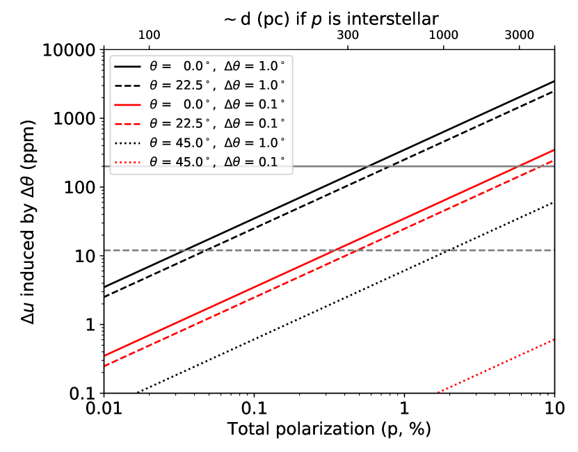
Because interstellar polarization increases with distance, the number of objects that can be studied long term at high precision is severely limited and many rarer stellar types are completely unavailable. To enable the discovery of new polarigenic mechanisms this must be remedied. To understand the scale of the problem, consider polarization due to binary reflection: in the Spica system this has an amplitude of 200 ppm (Bailey et al., 2019) – represented by the solid grey horizontal line in Fig. 1. A 1∘ error in can produce errors in the Stokes parameters at that level at a distance of 300 pc ( 0.55%). The predicted Rayleigh scattering signal from hot-Jupiter exoplanet atmospheres in the combined light of star and planet is, at best, of order 10-20 ppm (Bott et al., 2016, 2018; Bailey et al., 2021). Similarly, the pulsation-driven polarization produced in the Cep variable Cru is just 12 ppm (Cotton et al., 2022b) (dashed grey line). For these signal levels a 1∘ error can be significant even within 100 pc of the Sun. Improving precision in to 0.1∘ displaces the threshold for hot-Jupiter or Cru like polarization to 300 pc, and Spica like polarization to 3000 pc.
Our first objective in this paper is to establish mean offsets between the standards. As it stands, varying the mix of standards changes the calibration. Presumably, zero point differences between different observers are a source of imprecision. The second objective is to provide an updated assessment of the position angle variability of established polarization standards – especially long-term variability – and in so doing determine which, if any, are suitable for achieving 0.1∘ precision.
This paper is structured as follows: Sec. 2 provides background on each of the high polarization standard stars studied. Sec. 3 describes our observations; the analysis of which is carried out in Sec. 4. In Sec. 5 we discuss the implications of the results. Of particular note, Sec. 5.4 shows the impact of each correction we made. While, Sec. 5.5 lists six specific recommendations for observers relating to the acquisition, processing and reporting of position angle data. The conclusions are presented in Sec. 6. Appendices A, B, and C detail literature data and calibration details. For easy reference, Appendix D lists a selection of symbols used through the paper.
2 High polarization standard stars
| Standard | R.A. | Dec. | Plx. | SpT | GCVS | ||||||||||
| (HD) | (Alt.) | (ICRS J2000) | (mas) | (mag) | (mag) | (mag) | (mag) | (%) | (m) | () | (m) | ||||
| 7927 | Cas | 01 20 04.9 | 58 13 54 | 0.21 | F0 Ia | 5.66 | 4.98 | 0.51 | 3.11 | 3.31 | 0.507 | 0.85 | 93.0 | 5.7 | |
| 23512 | BD23 524 | 03 46 34.2 | 23 37 26 | 7.33 | A0 V | 8.44 | 8.09 | 0.37 | 3.27 | 2.29 | 0.600 | 1.01 | 30.4 | 3.6 | |
| 43384 | 9 Gem | 06 16 58.7 | 23 44 27 | 0.55 | B3 Iab | 6.70 | 6.25 | 0.57 | 3.06 | 3.06 | 0.566 | 0.97 | 170.0 | 2.6 | Cyg |
| 80558 | LR Vel | 09 18 42.4 | 51 33 38 | 0.54 | B6 Ia | 6.47 | 5.93 | 0.59 | 3.25 | 3.34 | 0.597 | 1.00 | 163.3 | 1.4 | Cyg |
| 84810 | Car | 09 45 14.8 | 62 30 28 | 1.98 | G5 Iab | 5.09 | 3.75 | 0.18 | 3.72 | 1.62 | 0.570 | 0.96 | 100.0 | 0.0 | Cep |
| 111613 | DS Cru | 12 51 18.0 | 60 19 47 | 0.45 | A1 Ia | 6.10 | 5.72 | 0.40 | 3.72 | 3.14 | 0.560 | 0.94 | 80.8 | 0.0 | Cyg: |
| 147084 | Sco | 16 20 38.2 | 24 10 10 | 3.71 | A4 II | 5.40 | 4.57 | 0.75 | 3.67 | 4.41 | 0.684 | 1.15 | 31.8 | 0.0 | |
| 149757 | Oph | 16 37 09.5 | 10 34 02 | 8.91 | O9.5 Vn | 2.58 | 2.56 | 0.32 | 2.93 | 1.45 | 0.602 | 1.17 | 127.2 | 5.0 | Cas |
| 154445 | HR 6353 | 17 05 32.3 | 00 53 31 | 4.02 | B1 V | 5.73 | 5.61 | 0.40 | 3.03 | 3.66 | 0.569 | 0.95 | 90.0 | 0.0 | |
| 160529 | V905 Sco | 17 41 59.0 | 33 30 14 | 0.54 | A2 Ia | 7.87 | 6.66 | 1.29 | 2.94 | 7.31 | 0.543 | 0.91 | 20.0 | 3.5 | Cyg: |
| 161056 | HR 6601 | 17 43 47.0 | 07 04 47 | 2.44 | B1.5 V | 6.68 | 6.32 | 0.60 | 3.11 | 4.01 | 0.584 | 0.96 | 67.3 | 1.5 | |
| 161471 | Sco | 17 47 35.1 | 40 07 37 | 1.69 | F2 Ia | 3.49 | 2.99 | 0.26 | 2.42 | 2.28 | 0.560 | 0.94 | 2.4 | 1.1 | |
| 183143 | HT Sge | 19 27 26.6 | 18 17 45 | 0.43 | B7 Iae | 8.08 | 6.86 | 1.24 | 3.16 | 6.16 | 0.550 | 1.15 | 179.2 | 0.0 | Cyg: |
| 187929 | Aql | 19 52 28.4 | 01 00 20 | 3.67 | F6 Ib+ | 4.61 | 3.80 | 0.16 | 3.10 | 1.73 | 0.552 | 0.93 | 93.7 | 7.3 | Cep |
| 198478 | 55 Cyg | 20 48 56.3 | 46 06 51 | 0.54 | B3 Ia | 5.28 | 4.86 | 0.54 | 2.89 | 2.75 | 0.515 | 0.88 | 3.0 | 0.0 | Cyg |
| 203532 | HR 8176 | 21 33 54.6 | 82 40 59 | 3.44 | B3 IV | 6.51 | 6.38 | 0.32 | 3.05 | 1.39 | 0.574 | 0.86 | 126.9 | 2.4 | |
| 210121 | HIP 109265 | 22 08 11.9 | 03 31 53 | 3.00 | B7 II | 7.84 | 7.68 | 0.35 | 2.22 | 1.38 | 0.434 | 0.73 | 155.1 | 8.6 | |
Notes – Aql has an SB companion classified computationally as B9.8 V. Photometric data and astrometric data, presented in sexagesimal IRCS J2000, are taken directly from SIMBAD. For the origin/derivation of position angle data see Appendix A. Note that is given for the SDSS band and a 2020 equinox. For the origin of Serkowski fit parameters, reddening data and spectral type references see Appendix B. The final column has the variability type as given in the General Catalog of Variable Stars (GCVS, Samus’ et al., 2017), where a colon indicates some uncertainty; HD 160529 is elsewhere classified as a Luminous Blue Variable (LBV) star (e.g. Stahl et al., 2003), and HD 149757 as an Oe star (e.g. Negueruela et al., 2004) and a Cep star (e.g. Hubrig et al., 2011).
Very bright high polarization standards are rare. The large distances required for significant interstellar polarization mean that only stars with small absolute magnitudes are bright enough. As a result, most standards trace their lineage to the first decades of stellar polarimetric study when the first bright star surveys were being conducted. In particular, the most used standards are drawn from a recommended list first published by Serkowski (1974a). The parameters for those stars were all refined in Serkowski et al. (1975). Other observers have occasionally added to (or subtracted from) this list, according to their needs, but have largely applied the same selection criteria. There are perhaps as many as two dozen standards in irregular use, depending on what brightness criteria are applied. These stars are far from evenly distributed across the sky. Overwhelmingly the standards are located in dusty regions fairly close to the Sun, such as the Sco-Cen association; the few that aren’t can be very important. For instance, Matsumura et al. (1997) described reports of variability in HD 43384 as a “serious problem,” stressing that there was no bright alternative within 6 h right ascension in the northern hemisphere.
We have largely worked from southern mid-latitudes, and so most stars we report on here are accessible primarily from there, but the transportation of an instrument to the Monterey Institute for Research in Astronomy (MIRA), has allowed us to add a number of northern stars. The standard stars in this study all appear in the catalogs of Serkowski et al. (1975), Hsu & Breger (1982), and/or Bagnulo et al. (2017); their properties are summarised in Table 1. They are all either well established standards or have been used as such in making observations with the High Precision Polarimetric Instrument (HIPPI) and other HIPPI-class polarimeters. Appendices A and B provide references and describe, in meticulous detail, how we came to favour the tabulated polarization and reddening properties. The co-ordinates and magnitudes for each standard given here – that define which telescopes they are accessible to – are taken directly from SIMBAD. Below is an account of other pertinent details, including variability found by other methods that might portent polarimetric variability, as well as a detailed account of claims and counter-claims of polarimetric variability for each star.
2.1 HD 7927
HD 7927 ( Cas) is a bright yellow supergiant star of spectral type F0 Ia (Gray et al., 2001) that is likely, though not conclusively, a member of the NGC 457 moving group (Eggen, 1982; Rosenzweig & Anderson, 1993). It has two notable visual companions, the brightest companion ( Cas) is 7.04, 132.8 away, and the closest companion is a 12.3 at 48.4 separation (Mason et al., 2001). Small amplitude variations with no defined period have been found in RV (Adams et al., 1924; Arellano Ferro et al., 1988)444Arellano Ferro et al. (1988) state HD 7927 is not in Adams et al. (1924). However, Adams et al. (1924) list it according to its catalogue number in Boss (1910)’s Preliminary General Catalogue of 6,188 Stars. His son’s later General Catalogue of 33,342 Stars (Boss et al., 1936) uses different catalogue numbers for the same stars, however both catalogues are generally referred to by the prefix “Boss.” We believe this to be the source of confusion. and in photometry by Percy (1989), who note that the photometric variations are too small compared to RV to indicate Cepheid-like behaviour.
First measurements of HD 7927’s polarization were made by Hiltner (1951). The star was not found to be variable by Coyne (1972) but he did note its as anomalous. No variability was found by Hsu & Breger (1982), whose claimed detection thresholds are 0.01 per cent in and 0.2∘ in . Wavelength dependence of in HD 7927 has been observed on multiple occasions (Gehrels & Silvester, 1965; Coyne & Gehrels, 1966; Hsu & Breger, 1982) but only Dolan & Tapia (1986) found that the wavelength dependence varied from night to night; they emphasize this as critically problematic for a position angle standard. Dolan & Tapia (1986) also found variable. Furthermore, (Bastien et al., 1988) found HD 7927 to be variable in both and , although the results of this paper are heavily criticized and this result refuted by Clarke & Naghizadeh-Khouei (1994). Earlier Naghizadeh-Khouei (1991) had described this star as displaying “definite polarization variability” both in , and in in band (but not in in band) based on his own observations.
2.2 HD 23512
HD 23512 (BD23 524) is an A0 V type star (Fitzpatrick & Massa, 2007) and is a member of the Pleiades cluster (Abt & Levato, 1978). The star has a companion, discovered by lunar occultation, with a brightness difference of 2 mag and a separation of (Mason et al., 2001) or (Torres et al., 2021). It has been a candidate for having a variable RV (Smith & Struve, 1944) but this was not confirmed by Abt et al. (1965). The star has also been a double line candidate (Liu et al., 1991) but this was not corroborated by Torres (2020). The polarization of HD 23512 was found not to be variable by Hsu & Breger (1982). It is described as “clearly” variable in both and by Bastien et al. (1988), which was refuted by Clarke & Naghizadeh-Khouei (1994).
2.3 HD 43384
HD 43384 (9 Gem) is of spectral type B3 Ib (Rachford et al., 2009) classified as an Cyg variable star (ESA, 1997). Hsu & Breger (1982) found that the star’s polarization angle is variable at a level of 0.8 0.2∘ on the short term, with larger long term variations apparent (; % over a decade). Coyne (1972) had previously described variability around thrice as much in both and . Matsumura et al. (1997) found that the polarization variability (; ) was phase locked with the 13.70 day period observed in Hipparcos photometry (ESA, 1997). In contrast Dolan & Tapia (1986), though noting an extreme found neither that parameter to be complex nor to be variable.
2.4 HD 80558
HD 80558 (LR Vel) is a B6 Ia supergiant (Houk, 1978) with prominent photometric variability (van Genderen et al., 1989). The polarization of HD 80558 was first studied by Serkowski & Robertson (1969) and it has been used as a high polarization standard since then. Dolan & Tapia (1986), in comparing their data to Serkowski (1974a)’s, found no significant difference in or . Hsu & Breger (1982) also reported no variability. Bastien et al. (1988) found HD 80558 to have variable polarization over 35 nights of observation. This result was refuted by Clarke & Naghizadeh-Khouei (1994)’s reanalysis of Bastien et al. (1988)’s data.
2.5 HD 84810
HD 84810 ( Car) is a classical Cepheid variable with a spectral type that ranges from F8–G9 (Albrecht, 1921) and a period of 35.5 days (Trahin et al., 2021). Owing to its brightness and proximity it has been extensively observed from ultraviolet (UV) to infrared (IR) wavelengths for more than a century (e.g. Bohm-Vitense & Love, 1994; Kervella et al., 2006). In principle the purely radial pulsations of a Cepheid variable should produce no polarization change (Odell, 1979), and HD 84810 has been found to be invariable in and by Hsu & Breger (1982), Bastien et al. (1988) and Clarke & Naghizadeh-Khouei (1994). Sensitive measurements by Bailey et al. (2023) show only small variations in of 0.023 0.005 per cent from 48 observations over about a year.
2.6 HD 111613
HD 111613 (DS Cru) is a supergiant of spectral type A2 Iab (Ebenbichler et al., 2022) and a member of NGC 4755 (Humphreys, 1978). Hsu & Breger (1982) find no variability for HD 111613 in or . Dolan & Tapia (1986) saw no change in over a four-year period (1980-84), but found and its wavelength dependence to be inconsistent between observing runs. Bastien et al. (1988) observed for 41 nights and saw significant variations in both and (, per cent) on a timescale of 32 days, a result confirmed by Clarke & Naghizadeh-Khouei (1994)’s reanalysis. Bastien et al. (1988) noted that the polarization was seen to vary slowly, and supposing a binary system, derived an inclination of based on an assumed a 64-day period.
2.7 HD 147084
HD 147084 ( Sco) is an A4 II bright giant (Martin et al., 1999) in Upper-Scorpius (de Geus et al., 1989). Small amplitude RV variations were measured by Levato et al. (1987) who state that this range may be due to intrinsic motions in the atmosphere. HD 147084 is noteworthy for being a standard for circular as well as linear polarization. It has a maximum fractional circular polarization of approximately 0.04 per cent at (Kemp, 1972), indicating that the light passes through at least two regions of the interstellar medium with differently aligned dust particles.
HD 147084 has substantial coverage in polarization data spanning ultraviolet to infrared wavelengths, owing to its large , making it particularly useful as a standard (Kemp, 1972; Martin et al., 1999). No variability in or was found by Hsu & Breger (1982) nor Dolan & Tapia (1986). In contrast, Bastien et al. (1988) find it to be variable in both and , a result refuted by Clarke & Naghizadeh-Khouei (1994). A small potential variability in of 0.028 0.008 per cent has been found by Bailey et al. (2023) from 108 observations over more than a year.
2.8 HD 149757
HD 149757 ( Oph) is a well-studied single star with an O9.5 V spectral type (Hubrig et al., 2011). Its rapid rotation velocity of 400 km/s causes it to lose mass through a strong wind (Hubrig et al., 2011), and gives rise to a variable surface temperature through its oblateness (Balona & Dziembowski, 1999). Periodic variability for this star has been noted in both photometry and spectroscopy (helium line profiles) consistent with a Cephei type classification (Hubrig et al., 2011). The spectral variability is likely the result of non-radial pulsations (Balona & Kambe, 1999), where these modes may be excited periodically by lower order modes (Walker et al., 2005). HD 149757 was one of ten O-type stars included in a study of polarimetric variability by Hayes (1975), from 12 observations over many weeks, he did not find it to be variable. Lupie & Nordsieck (1987) describe the star as nonvariable but caution they have few observations. McDavid (2000) carried out a study of nine O-type stars with variable winds, including HD 149757, using agglomerated data from 1949 to 1997; none exhibited statistically significant variability, but small amplitude, short term variability amongst the targets was hinted at by a multi-technique campaign.
2.9 HD 154445
HD 154445 (HR 6353) is a B1 V spectral type star (Reed, 2003); it has no identified companions (Eggleton & Tokovinin, 2008). The first reported polarimetric observations of HD 154445 were made by Hiltner (1951). Repeated observations at optical (e.g. van Panhuys Smith, 1956; Serkowski et al., 1975; Cikota et al., 2018) and near-infrared wavelengths (Dyck et al., 1971; Dyck & Jones, 1978) have demonstrated consistency in and . Hsu & Breger (1982) find the HD 154445 to be invariable in and . The star was claimed as variable in (but not ) at the 2- level by Bastien et al. (1988), but this was not borne out by reanalysis (Clarke & Naghizadeh-Khouei, 1994). Recently reported observations by Wiktorowicz et al. (2023) present little evidence for variability.
2.10 HD 160529
HD 160529 (V905 Sco) is a Luminous Blue Variable (LBV) of spectral type A2Ia (Stahl et al., 2003). It has a prolific history as a photometric and spectroscopic variable star (e.g. Wolf et al., 1974; Sterken et al., 1991). Decades of photometry from Sterken et al. (1991) show that the star’s magnitude dimmed by 0.5mag over 18 years. More recent AAVSO data spanning the last 20 years shows similar timescales of variability, with as much as a magnitude in brightness changes. A spectroscopic study by Wolf et al. (1974) highlighted many signatures that could likely be attributed to strong mass loss including line profile variations, line splitting, P-Cygni and inverse P-Cygni profiles. This large photometric and spectroscopic variability has likely led to the difficulties in classifying the spectral type; the presence of strong, sharp emission lines and H excess likely complicated it as well. Early classifications of HD 160259 included, A4 se (Merrill & Burwell, 1933), A2-3 Ia (Wallerstein, 1970), and A9 Ia (Houk, 1982).
2.11 HD 161056
HD 161056 (HR 6601) is a B1/2V star (O’Donnell, 1994). Telting et al. (2006) included it in a study looking for line profile variations associated with pulsation; none were indicated, albeit from a single observation. HD 161056 was first observed polarimetrically by van Panhuys Smith (1956) as part of her survey of interstellar polarization in the Southern Milky Way and it is often included in polarimetric studies of the interstellar medium (e.g. Piccone & Kobulnicky, 2022). Bastien et al. (1988) only suspected variability in but reported variability of 0.5∘, however later reanalysis calls into question this conclusion (Clarke & Naghizadeh-Khouei, 1994). Berdyugin et al. (1995) constrain any variability to 1∘.
2.12 HD 161471
HD 161471 ( Sco) is a luminous red supergiant star of spectral type F2Ia (Houk, 1978; Gray & Garrison, 1989). It is a spectroscopic binary (Pourbaix et al., 2004) and has a 13th mag companion at 37 separation. It’s H line width probably indicates a weak stellar wind (Danks & Dennefeld, 1994). It is not a widely used position angle standard, but has been so utilized by Bailey et al. (2023) to calibrate the position angle of polarization in 20-cm PICSARR observations. They find potential variability in of 0.020 0.004 per cent from 18 observations spanning more than a year.
2.13 HD 183143
HD 183143 (HT Sge) is an extremely luminous hypergiant star of spectral type B7Iae (Chentsov, 2004). It was first found to have a high broadband polarization by Hall & Mikesell (1950), who described it as a “star of special interest.” Serkowski (1974a) later named it as a standard. Clemens & Tapia (1990) found their observations of it to be consistent with those of Serkowski et al. (1975) and Schulz & Lenzen (1983) claim its polarization as a function of wavelength is consistent with an interstellar origin. Spectropolarimetric data from Lupie & Nordsieck (1987) marks it as their least variable standard, but shows 0.40∘. However, Hsu & Breger (1982) convincingly showed HD 183143 exhibited polarimetric variability (, per cent) on a timescale of days to weeks, and Dolan & Tapia (1986) found that its character varied from night-to-night, along with itself.
2.14 HD 187929
HD 187929 ( Aql) is a classical Cepheid with spectral type F6 Ib-G4 Ib and a pulsational period of 7.18 d (Benedict et al., 2022). As the first Cepheid discovered (Pigott, 1785), it has been well-studied over the years, and perhaps most particularly during the era of space observations (Evans, 1991; Benedict et al., 2007; Evans et al., 2013). The current understanding is that it is a triple system containing, in addition to the Cepheid, a late-B close-in companion as well as an F-type companion lying some 0.66 from the primary. Polarimetric measurements of the star have focused on attempts to detect a magnetic field using spectropolarimetry to varying degrees of success (Borra et al., 1981; Plachinda, 2000; Wade et al., 2002; Grunhut et al., 2010). In linear polarization Hsu & Breger (1982) report a particularly large of , but no variability. Dolan & Tapia (1986) report measurements that differ by from Hsu & Breger’s, along with a complex behaviour not explainable by a two-cloud model, and they name intrinsic polarization as a possibility. Bastien et al. (1988) categorized HD 187929 as a suspected variable, but later retract this assessment (Bastien et al., 2007).
2.15 HD 198478
HD 198478 (55 Cyg) is a blue supergiant star of type B3 Ia and a prominent Cyg variable with asymmetric contraction varying over hours to days (Wilson, 1953). Periods of variability (in pressure, gravity, and modes) appear to correlate with—and are well-modelled by—mass loss episodes (Yadav & Glatzel, 2016; Kraus et al., 2015). HD 198478 may also experience macroturbulence from convection significant enough to contribute to measurable line broadening beyond that from rotation (Jurkić et al., 2011), which may further influence the consistency of some parameters like surface gravity.
Although it is widely used as a standard polarization star (e.g. Cox et al., 2007), large changes in the polarization of HD 198478 have been observed previously by Hsu & Breger (1982) and Wiktorowicz et al. (2023). In particular, Hsu & Breger (1982) saw changes in and of 1∘ and 0.06 per cent, respectively, within a short run – several days. They associated this variability with emission variability seen to occur on the same short time scale as reported by Underhill (1960) and Granes & Herman (1972). Dolan & Tapia (1986) also suspected variability, partly on the basis that their determination differed substantially from earlier literature but also because Treanor (1963) noted was unusually high for its location. Naghizadeh-Khouei (1991) describes its variability in and as “very obvious,” in particular reporting 4.8∘, but observing that is consistent from night-to-night. Naghizadeh-Khouei (1991) was critical of the statistical approach of some of the early polarimetric studies, and advocated use of the CDF to aid in matching the polarimetric mechanism to the observed variability. In this specific case he noted the similarity of the variability of this star to that of other supergiants, ascribing it to mass loss and the presence of a stellar wind.
2.16 HD 203532
HD 203532 (HR 8176) is a B3 IV subgiant in the constellation Octans. It is the southernmost standard in the current study with a declination of . With this latitude, it is placed close to the molecular clouds south of the Chamaeleon complex which are associated with the Galactic plane (Larson et al., 2000). Due to coordinate precession being larger for coordinates close to the celestial poles the position angle changes more over time than for the lower latitude stars (see Table 9). HD 203532 has no known companions nor is it a known variable star (Samus’ et al., 2017).
The first polarization measurement was made by Mathewson & Ford (1970). Later Serkowski et al. (1975) made four measurements yielding position angles between and in the band. It has not been reported to be variable, but measurements made by Bagnulo et al. (2017) and Bailey et al. (2020) with modern equipment disagree in by 2.6 0.9∘.
2.17 HD 210121
HD 210121 (HIP 109265) is a B-type star, sharing a line of sight with a single, high latitude cloud sitting pc from the Galactic plane (Welty & Fowler, 1992). The star is of uncertain spectral type, with several incongruent classifications having been assigned at different points in the literature. For example, its spectral type has been listed as B3 V (Welty & Fowler, 1992; Larson et al., 1996), B3.5 V (Siebenmorgen et al., 2020; Krełowski et al., 2021), B5-6 V (de Vries & van Dishoeck, 1988), B7 II (Valencic et al., 2004; Fitzpatrick & Massa, 2007; Bagnulo et al., 2017; Piccone & Kobulnicky, 2022), and B9 V (Voshchinnikov et al., 2012). On the whole, a critical reading of the literature suggests to us that an earlier spectral type is more likely, however we have opted to use the B7 classification in this work, since this is what was used for determining the Serkowski parameters. With the foreground cloud characterised by a high abundance of small grains, HD 210121 is often cited with reference to its extremely low and high UV extinction.
3 Observations
The data for this work comes from 88555There have been 91 observing runs with the HIgh Precision Polarimetric Instrument (HIPPI) and its derivatives (referred to as HIPPI-class instruments) to date. One test run with Mini-HIPPI on the Penrith telescope used Achernar in emission (HD 10144; ) for position angle calibration and is not included. Another two constituted the first re-commissioning run for the second HIPPI-2 at MIRA’s OOS and are not considered reliable due to issues with the modulator and rotation stage (see Cotton et al., 2022b). observing runs (or sub-runs666A new mounting of the instrument within an otherwise contiguous run.) on six different telescopes using four different HIPPI-class polarimeters of three different designs, spanning 10 years of operation. It includes every observation we have made of the 17 different standards listed in Table 1 during these runs. For 5 standards our data spans the full (almost) 10 years, two stars (HD 7927 and HD 198478) were observed from the northern site for only a year, the HD 43384 data span is only slightly longer than a year, every other star has a multi-year data set, most of which are at least 5 years. Many of the observations were made solely for the purpose of calibration, and some multi-band observations were made to check the modulator efficiency (see Appendix C). However, from June 2020 a number of observing runs were made specifically for this work.
The six telescopes observed with were the 3.9-m Anglo-Australian Telescope (AAT) at Siding Spring Observatory, the Penrith 60-cm (24-in) telescope at Western Sydney University (WSU), a 14-inch Celestron C14 at UNSW Observatory (UNSW), a Celestron 9-inch telescope at Pindari Observatory in suburban Sydney (PIN), the 36-in telescope at MIRA’s Oliver Observing Station (OOS), and the 8.1-m Gemini North Telescope (GN).
The four HIPPI-class polarimeters include the original HIPPI (Bailey et al., 2015), Mini-HIPPI (Bailey et al., 2017), and two different HIPPI-2 units (differentiated by the hemispheres they operated in, Bailey et al., 2020; Cotton et al., 2022a). They are dual-beam777Several high polarization standard observations from one run (N2018JUN) were made with only one channel due to a cabling failure. aperture photo-polarimeters that share common design elements, namely a ferro-electric crystal modulator operating at 500 Hz and optimised for blue wavelengths; a Wollaston (or Glan-Taylor) prism analyzer; and modern, compact photo-multiplier tube detectors (PMTs). The PMTs are manufactured by Hamamatsu; we mostly used blue (B) sensitive units (Nakamura et al., 2010), but a few observations were also made with PMTs with a redder response curve (designated R). Most observations were made in the SDSS filter or unfiltered (Clear), but a range of other filters were used as described in Appendix C.
Each of these instruments measure only a single Stokes parameter at once. To measure the other Stokes parameter, the instrument is rotated through 45∘. With HIPPI this was accomplished with the AAT’s Cassegrain rotator. The other instruments instead used their own instrument rotator. In practice an observation was actually made up of four measurements: at angles of 0, 45, 90 and 135∘, where the perpendicular measurements are combined in a way that minimises any instrumental contribution to the polarisation.
A database containing a summary of the instrument and telescope set-up for each run, and the details of every high polarization standard observation in machine readable format is available at CDS via anonymous ftp to cdsarc.u-strasbg.fr (130.79.128.5) or via https://cdsarc.cds.unistra.fr/viz-bin/cat/J/MNRAS or on MIRA’s website at http://www.mira.org/research/polarimetry/PA. The catalogue contains both the and Clear (unfiltered) observations analysed in the main part of the paper, as well as those made in other bands used for calibration in Appendix C (583 observations in total). Note that only the errors derived from the internal statistics of the observation are reported in the catalogue, for an assessment of accuracy see initially, Appendix C.4, then Sections 4.3 and 4.4.
3.1 Reduction
Standard reduction procedures for HIPPI-class polarimeters are described by Bailey et al. (2020). These include a bandpass model that takes account of the spectral type of the target. For this work we have re-evaluated and updated the modulator calibrations to improve the accuracy of this procedure (see Appendix C). Here we improve the bandpass model by including the expected polarization and reddening of the standards (given in Appendix B), the computer code is adapted from the PICSARR reduction (Bailey et al., 2023).
The telescope polarization (TP) is measured by many observations of low polarization standard stars assumed to be unpolarized. The full list of standards used is: Aql, Boo, Boo, Boo, Cet, Cen, CMa, CMi, Hyi, Lac, Leo, Ser, Tau and Vir. Aside from CMi, all of the additions from those listed in Bailey et al. (2020) have been restricted to northern hemisphere use. The standard bandpass model is applied prior to the straight average of the standard measurements in each band being taken, then these values are vector subtracted from all the other observations. Aside from run N2018JUN (see Bailey et al., 2020), the TP never exceeded 170 ppm in the band, and varied by typically 10s of ppm or less between bands. Typical TP levels for the telescopes we observed with can be seen in Bailey et al. (2017, 2020) and Cotton et al. (2022b). The nominal errors of this process are mostly less than 10 ppm with larger uncertainties occurring only for some of the smaller telescope runs. These errors are wrapped into the observational errors on an RMS basis – and for the most part are negligible.
The telescope position angle is usually calibrated as the straight average difference between the expected and observed position angles of standards observed in a or Clear filter. The nominal position angles, of the standards have been redetermined from the literature in Appendix A. The expected position angles include some corrections to these. The two most important are related to the change in position angle with wavelength, , and the precession of the co-ordinate system – these are also described in Appendix A.
The precession turns out to be particularly important. Stars in the North precess positively in , and vice versa for those in the South – with typical values for being several tenths of a degree per century. The literature values for were first established for some standards more than 50 years ago. Failing to account for precession can artificially induce a degree or more difference between some pairs of standards.
Here we also apply a correction for the Faraday rotation of polarization (Faraday, 1846) by the atmosphere in the presence of the Earth’s magnetic field. This step is recommended by Clarke (2010) when , which many of our measurements nominally surpass. Though never observed, the possible impacts of Faraday rotation on ground-based astronomical polarimetry have been discussed for nearly a century (Lyot, 1929; Serkowski, 1974b; Hsu & Breger, 1982; Clarke, 2010). Here we make the same simplifying assumptions as Hsu & Breger (1982), namely that the Earth’s magnetic field is aligned to geographic poles, and employ,
| (6) |
where is the component of the magnetic field (0.5 Gauss) parallel to the line of sight, the scale height of the atmosphere equal to 80000 cm, the airmass, and the Verdet constant, which is dependant on wavelength. West & Carpenter (1963) give as 6.27 arcmin/Gauss/cm for the air at standard temperature and pressure at 567 nm, and we derive the values at other wavelengths by scaling and extrapolating from Figure 2 in Finkel (1964) – at 470 nm this gives 9.53 arcmin/Gauss/cm. At the airmasses of our observations, the correction never comes to much more than 0.01∘.
4 Analysis
4.1 Position Angle Precision by Instrument
Clarke & Naghizadeh-Khouei (1994)’s primary criticism of Bastien et al. (1988) was that measurements from different set-ups were combined in an unweighted way. To conduct a long term analysis we need to combine data from multiple (albeit similar) instruments across many sub-runs, where each corresponds to a new mounting of the instrument on the telescope. This task requires some care. So, before we attempt it, we first seek an understanding of the variability attributable to different telescope/instrumental set-ups.
In Table 2 the standard deviation of , , of repeat observations in the same filter (limited to or Clear) of the same star within a sub-run is determined; such observations are directly comparable with each other. The table reports the median standard deviation, , of each set of observations, where the number of observations, ; and the median of , a metric designed to determine the scatter independent of known noise sources,
| (7) |
where is the measured uncertainty derived from the internal statistics of our measurements, it is largely photon-shot noise but also incorporates other noise sources associated with seeing and the detector888There is also a very small contribution ascribed to centering imprecision (see Bailey et al., 2020), which we include throughout this paper in but otherwise neglect to mention in order to simplify discussion..
It should be noted that this approach is strictly only valid for a Gaussian distribution, and is not Gaussian. However, it approaches Gaussian at high signal-to-noise, i.e , and in our case , typically.
| Instrument | Telescope | |||
| (∘) | (∘) | |||
| HIPPI | AAT | 5 | 0.070 | 0.068 |
| HIPPI-2 | AAT | 33 | 0.082 | 0.077 |
| HIPPI-2 | WSU-24 | 3 | 0.144 | 0.139 |
| HIPPI-2* | MIRA-36 | 8 | 0.196 | 0.186 |
| M-HIPPI | UNSW-14 | 5 | 0.292 | 0.282 |
| M-HIPPI | PIN-9 | 25 | 0.483 | 0.474 |
| HIPPI-2* | WSU/MIRA | 11 | 0.168 | 0.153 |
| HIPPI-2† | Gemini Nth | 4 | 0.240 | 0.173 |
Notes – is the number of sets. * HD 198478 removed; includes observations only until to 2023-09-01. Observation sets are combined , 500SP and Clear observations.
The different instruments had different rotation mechanisms, which is likely to contribute to scatter in . HIPPI used the Cassegrain rotator of the AAT to move position angle, while HIPPI-2 and Mini-HIPPI have their own instrument rotator. HIPPI-2’s rotator is a heavy-duty precision component, and on the AAT the value for is small. Mini-HIPPI’s rotator is not as well made, so the lower precision for Mini-HIPPI was expected. Additionally, the Pindari telescope, unlike the others, is not on a fixed mount so is susceptible to external forces, e.g. wind, incidental operator intervention.
The smaller telescopes do not have as good a value for as the AAT. Potential mechanical explanations would be a slight polar misalignment or play in the mounting. However, the number of observation sets is small, and so the difference could just be a result of which stars were used in the measurements. For the MIRA-36 this is likely to be a factor since, proportionally more standards were observed which are robustly reported as variable in the literature (and we have excluded HD 198478 from this part of the analysis because it especially biases the results). More reliable standards make up a larger majority of the sets for the other telescope/instrument combinations. To get a more robust measure for the two smaller HIPPI-2 compatible telescopes, we combine their data below the midline of Table 2.
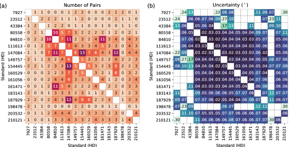
When a pair of standards are both observed during the same sub-run, that counts as one pair. Only observations made with the B PMT were used. In both panels the information is mirrored for easy reference.
We do not have repeat observations of any standards during the Gemini North run (N2018JUN). Hence, to provide a representative figure we make observation sets for four stars by combining , 500SP and one Clear observation, wavelength corrected using our bandpass model according to the relations in Appendix A. This is less than ideal because the observations were taken sequentially, but they do at least probe a small range of paralactic angles for the Alt-Az mount. This is important because the telescope polarization during the run was large – probably owing to an inhomogenously aluminized secondary (Wiktorowicz et al., 2023) – and the position angle of its wavelength dependence was not well determined (Bailey et al., 2020).
4.2 Relative position angles using the Co-ordinate Difference Matrix
Informed by the relative performance of the instruments, we now seek to re-establish values for our standards using our data to facilitate literature comparisons. We use a co-ordinate difference matrix (CDM, Baechler et al., 2020) approach to combine data from sub-runs where at least two standards were observed in (with the B PMT). Using a single filter reduces the data available, but ensures uncertainties in wavelength effects are minimised. For reasons explained in Sec. 4.3, we have also removed the Pindari observations from this calculation.
A relatively new tool, CDMs are similar to a Euclidian Distance Matrices (EDM, Dattorro, 2005) and are finding applications in a number of different fields (e.g. Mozaffari et al., 2019; Krekovic, 2020; Liu et al., 2023; Chen et al., 2024). The CDM algorithm optimally calculates the relative mean differences between objects by combining such information from pairs of points. The algorithm is applicable even when the matrix is incomplete, i.e. when measurements do not exist for every object pair. Our application requires a weighted 1-dimensional CDM. From Baechler et al. (2020), algebraically, the CDM, is made up of elements , i.e. the differences between points and . We have a noisy CDM,
| (8) |
where is a noise matrix and the weight matrix. To optimally recover the set of points that generated it, the solution is
| (9) |
where and , where is the all-one vector and
| (10) |
The first point is then fixed to zero in the algorithm by removing the first point in and along with the first row and column of and likewise for all the corresponding matrices. From this process we take the nominal errors on the recovered points to be,
| (11) |
Here, our terms are values, and we calculate the weights using the root-mean-square (RMS) sum of and for each measurement. Where multiple observations of a standard have been made during a sub-run, we take the error-weighted-average, and thus also the resulting RMS-error for the weight calculation. The runs are combined in the same way. The result therefore makes no account of stellar variability – only mean position angles are calculated.
Figure 2(a) shows the number of object pairs used in the calculation and 2(b) the associated standard errors (where the weights are the inverse of the error squared). It should be noted that this does not match the number of observations because only a single agglomerated measurement is made per sub-run for a given standard, single-standard sub-runs are discarded, and because more standards were observed in some runs than others.
The results of the CDM procedure are presented in columns 6–10 of Table 3 where the standard error, , given in column 7 is the error in the mean given in column 6; this does not account for the error in the zero point of the co-ordinate system nor does it describe the distribution of values. Columns 9 and 10 are the weighted standard deviation of , , and the average error, (which is equal to ) after calculation of using the newly determined values of for each standard. Column 9 may be compared to column 5, which is the unweighted standard deviation after calibration of instead using – the way calibration of has previously been done for HIPPI-class instruments. It can be seen that the CDM-derived is reduced for most stars compared to the previous method. Our and terms are the equivalent of Bastien et al. (1988)’s and respectively.
| 1 | 2 | 3 | 4 | 5 | 6 | 7 | 8 | 9 | 10 | 11 | 12 | 13 | 14 | 15 | 16 | 17 | 18 |
| Co-ordinate Difference Matrix | Iterative fitting result | ||||||||||||||||
| Standard | Sig. | ||||||||||||||||
| (HD) | (∘) | (∘) | (∘) | (∘) | (∘) | (∘) | (∘) | (∘) | (∘) | (∘) | (∘) | (∘) | () | (∘) | (ppm) | ||
| 7927 | 10 | 3 | 93.0 | 0.331 | 93.187 | 0.032 | 0.187 | 0.341 | 0.161 | 93.165 | 0.069 | 0.165 | 0.344 | 0.170 | 2.1 | 0.321 | 367 |
| 23512 | 7 | 5 | 30.4 | 0.335 | 30.719 | 0.024 | 0.319 | 0.262 | 0.104 | 30.706 | 0.064 | 0.306 | 0.273 | 0.128 | 2.1 | 0.256 | 191 |
| 43384 | 11 | 3 | 170.0 | 0.269 | 170.309 | 0.021 | 0.309 | 0.234 | 0.099 | 170.295 | 0.049 | 0.295 | 0.199 | 0.115 | 1.7 | 0.167 | 171 |
| 80558 | 21 | 17 | 163.3 | 0.325 | 162.484 | 0.011 | 0.816 | 0.360 | 0.086 | 162.512 | 0.045 | 0.788 | 0.442 | 0.102 | 4.4 | 0.384 | 420 |
| 84810 | 33 | 20 | 100.0 | 0.321 | 99.989 | 0.010 | 0.011 | 0.191 | 0.086 | 99.997 | 0.019 | 0.003 | 0.132 | 0.098 | 1.3 | 0.110 | 60 |
| 111613 | 17 | 10 | 80.8 | 0.366 | 80.835 | 0.011 | 0.035 | 0.372 | 0.083 | 80.836 | 0.034 | 0.036 | 0.317 | 0.096 | 3.1 | 0.266 | 281 |
| 147084 | 53 | 30 | 31.8 | 0.315 | 32.015 | 0.009 | 0.215 | 0.195 | 0.091 | 32.028 | 0.018 | 0.228 | 0.141 | 0.110 | 1.4 | 0.118 | 155 |
| 149757 | 15 | 8 | 127.2 | 0.374 | 126.200 | 0.012 | 1.000 | 0.212 | 0.092 | 126.218 | 0.032 | 0.982 | 0.252 | 0.104 | 1.9 | 0.211 | 98 |
| 154445 | 24 | 16 | 90.0 | 0.342 | 89.976 | 0.011 | 0.024 | 0.190 | 0.092 | 89.985 | 0.022 | 0.015 | 0.132 | 0.109 | 1.1 | 0.110 | 134 |
| 160529 | 11 | 8 | 20.0 | 0.637 | 18.749 | 0.013 | 1.251 | 0.582 | 0.083 | 18.748 | 0.083 | 1.252 | 0.659 | 0.099 | 6.7 | 0.640 | 1604 |
| 161056 | 9 | 6 | 67.3 | 0.236 | 67.982 | 0.013 | 0.682 | 0.090 | 0.084 | 68.034 | 0.024 | 0.734 | 0.098 | 0.091 | 1.1 | 0.082 | 108 |
| 161471 | 10 | 6 | 2.4 | 0.314 | 2.060 | 0.013 | 0.340 | 0.153 | 0.081 | 2.087 | 0.027 | 0.313 | 0.147 | 0.089 | 1.7 | 0.123 | 94 |
| 183143 | 7 | 5 | 179.2 | 0.713 | 179.323 | 0.018 | 0.123 | 0.777 | 0.096 | 179.299 | 0.121 | 0.099 | 0.827 | 0.111 | 8.0 | 0.819 | 1710 |
| 187929 | 27 | 17 | 93.7 | 0.457 | 93.711 | 0.013 | 0.011 | 0.234 | 0.096 | 93.703 | 0.037 | 0.003 | 0.288 | 0.127 | 2.2 | 0.241 | 142 |
| 198478 | 12 | 2 | 3.0 | 0.660 | 2.474 | 0.031 | 0.526 | 0.643 | 0.161 | 2.417 | 0.095 | 0.583 | 0.647 | 0.170 | 3.8 | 0.628 | 595 |
| 203532 | 7 | 6 | 126.9 | 0.263 | 124.328 | 0.017 | 2.572 | 0.253 | 0.095 | 124.360 | 0.039 | 2.540 | 0.201 | 0.107 | 1.8 | 0.175 | 81 |
| 210121 | 8 | 6 | 155.1 | 0.282 | 153.836 | 0.019 | 1.264 | 0.255 | 0.123 | 153.903 | 0.049 | 1.197 | 0.287 | 0.132 | 2.0 | 0.264 | 126 |
Notes – Top row gives column numbers for easy reference. Analyses in Sec’s 4.2 and 4.3 correspond to columns 6–10 and 11–18 respectively, whereas columns 4 and 5 correspond to ordinary calibration procedures. The symbols and denote the number of observations and subruns, respectively, from which data is drawn for each standard. The literature values of position angle are denoted , whereas are the determined values from our analyses and, as elsewhere, given for a 2020 equinox; correspondingly is the nominal error on the determination from Equation 11 (effectively the error on the mean), is the difference between and ; is either the unweighted (column 5) or error-weighted (columns 9 and 14) standard deviations of position angle measurements after recalibration, and is the average of all the nominal position angle errors for each standard. The scatter attributed to variability on each star is fit value , Sig. the significance of that value (note that observations with larger errors are down-weighted in its calculation), and the minimum polarization needed to shift by if it acted perpendicular to the interstellar polarization. Note that (see the text of Sec. 4.3 for details). The absolute co-ordinate system uncertainty, not included in the reported uncertainties is 0.177∘.
The CDM only calculates the relative position angles of the standards (the value of the first listed object in the matrix is arbitrarily set to zero, so that represents the difference from it for each standard). For the absolute value we have calculated and applied an offset, , based on the literature values (as given in Table 9). Here is calculated by finding the median difference between the determined, , and the literature, values,
| (12) |
We estimate the error in by this method to be 0.177∘. In this case we calculated errors as the RMS sum of the values in Table 3 and 0.5∘ which we consider an appropriate typical uncertainty in the original literature measurements999The claimed accuracy is sometimes better than this. Hsu & Breger (1982) state 0.2∘ precision for instance, but we have taken an average of their work and others, and none estimate an error associated with the zero point offset.. HD 203532 is removed from the calculation as an obvious outlier.
An alternative method for determining would be to use the error-weighted average difference,
| (13) |
where the is the weight of the th element, equal to the inverse of the error squared. Hsu & Breger (1982) used this method to tie their measurements to those of Serkowski (1974a).
Calculating using Equation 13 rather than Equation 12 results in all the values in Table 3 being shifted by , which is not so different from the zero point uncertainty calculated above. We prefer the median approach to mitigate sparse sampling of potentially variable objects. These values describe the possible offset of our entire network of standards but bare no relevance for their relative position angles.
4.3 Estimating stellar variability in
In Sec 4.1 we estimated the uncertainty associated with each instrument/telescope combination, we now wish to do the same for each standard star, . A first step is to determine the (error weighted) standard deviation of position angles from their expected values for each standard – after re-calibrating for each run – these are the values in column 9 of Table 3. The general formula for weighted standard deviation is (Heckert & Filliben, 2003),
| (14) |
where is the weighted mean, the weights on each element , is the number of non-zero weights101010, where is the number of zero weighted terms., and the term comes about from Bessel’s correction to the variance, applied when the population mean is being estimated from the sample mean.
However, estimating in this way is very crude because depends on the weighted means of each observation for each run. Typically, each run contains only a handful of measurements where we have considered each standard to be as good as any other. If just one star is variable and significantly different to its assumed value of , that will shift the measurements of every other star in the run. The very parameters we aim to determine are corrupted by assuming them to be zero in the first instance.
To overcome this problem we employ a scheme that iteratively fits for : For this we use SciPy’s optimize function, employing the Sequential Least SQuares Programming Optimizer (SLSQP), to minimise a function ,
| (15) |
where is given by,
| (16) |
where is the degrees of freedom, equal to less the number of fit parameters, is the difference between the observed and expected value and the uncertainty associated with each measurement after re-calibration, which has four contributions,
| (17) |
is the measured uncertainty, as in equation 7; and are the standard deviations of the variability (errors) associated with the telescope/instrument set-up and the star being observed, respectively, and is the RMS error in the determined telescope zero point for the run (which, for each run, is derived from the other three terms).
However, depends on the values we assign for each star. The assignments are made using the CDM algorithm, which in turn depends upon the uncertainty assigned to each observation. Our assignments in Sec 4.2 are made, essentially, with . Therefore our fit function incorporates a recalculation of the CDM-derived assignments based on the current values of the fit parameters.
We found that the fit function was prone to getting stuck in local minima, leading to some values of being inconsistent with the subsequently calculated values of . This occurs because the CDM calculates only one value per star per run, and the fit function just demands a model where the sample variance is appropriately described, it does not care where the uncertainty is placed. To overcome this problem, we used the values determined after the fit as initial parameters for in subsequent fits and iterated until the values converged (i.e. did not change by more than 510 between subsequent iterations) though the changes are small after about the third iteration.
Initially we performed the analysis of Sec 4.2 using the same set of observations as in Sec. 4.1, but found that the three standards observed repeatedly at Pindari gave elevated values of compared to otherwise. We presume this to be due to the complications associated with not using a fixed mount, and so we excluded those observations from further analysis. We also removed the Clear observations; stellar variability is likely to have a wavelength dependence and we wanted an unbiased comparison between stars. We could not apply the same restriction in Sec. 4.1 since this would have left too few sets for some set-ups.
It follows that the uncertainty for each set-up could use some fine tuning. We tried fitting along with but this just transferred uncertainty from the set-ups to the stars, where the proportion was overly sensitive to the initial conditions. Though, if boundary conditions were enforced, the uncertainty transferred was mostly small. However, the ratios of to each other were typically only slightly changed, suggesting that the results of Sec. 4.1 are not biasing observations made with one set-up over another. It also means that if most stars are variable, our estimates of will underestimate the short term variability of the most stable stars. Ultimately we decided against fitting , as this represented the most conservative approach, and retain the values assigned in Sec. 4.1.
The results are given in columns 11-18 of Table 3. There are only minor changes in (column 11) compared to the pure CDM results (column 6). There are marked decreases in for the least variable stars, that are only partly offset by increases in the more variable stars. This result should be obvious because we are down-weighting the contributions of the most variable stars to achieve a more accurate determination of . The errors are increased because they now include a component associated with .
The significance of the determined we calculate (in column 16 of Table 3) by scaling each observation to the corresponding error, and then taking the error-weighted standard deviation. This is better than dividing by because it takes proper account of the different uncertainties associated with each observation. In column 17 the fit values of are given. Due to the nature of the fitting function . Five stars are found to be variable with 3 confidence – all of these are A or B type supergiants. Another four stars are seemingly variable only at the 2 level.
The final column of Table 3 is a calculation of polarization, following Equation 2, that would be required in to rotate by assuming . This allows the variability of the objects to be compared directly, independent of the interstellar polarization imparted by the ISM.
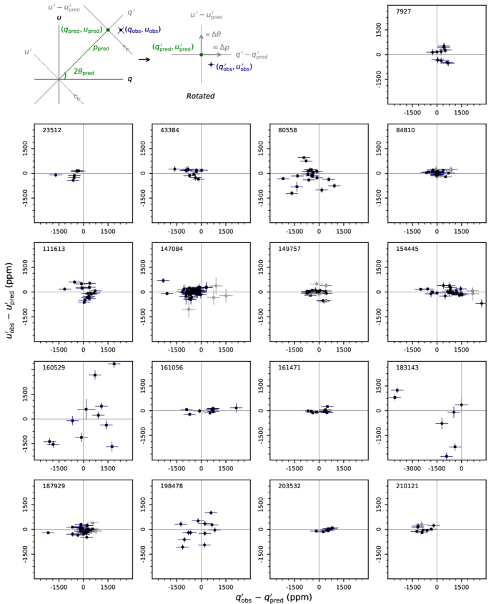
The and values are depicted graphically as the vertical and horizontal axes, respectively, of QU diagrams in Fig. 3 (full explanatory details are in the caption). The error bars plotted for are derived below in Sec. 4.4, but we present this figure here to make an important point: the improvements made in calibration have resulted in this being more accurate than our calibration. We have used three different modulators, where the performance of at least one of them has evolved over time, this affects modulation efficiency, including as a function of wavelength. Our ability to correct for efficiency changes is limited by the calibration data obtained (see Appendix C). But any change in modulator efficiency applies equally to each Stokes parameter so that the effects on are largely negated – especially in the bands most closely corresponding to the optimum operating wavelength of the modulator (i.e. the band, see Table 12) – the instrumental errors in come from other sources (largely mechanical), as already discussed in Sec. 4.1, and these are independently parameterised and accounted for. The consequences are easy to see in Fig. 3 – where the co-ordinate system is rotated, for each object, so that corresponds to changes in and to changes in – where the horizontal scatter is almost always greater than the vertical scatter. This means we cannot employ a CDF test reliably. However, where we see variability in we can be confident it is real, but if there is only scatter in this probably represents only instrumental variability.
4.4 Variability in
The statistics for all of the available observations are given in Table 4, except for those acquired at the Pindari observatory, which are given in Table 5. The Pindari observations have larger nominal (photometric) errors, but otherwise should be comparable.
| Standard | Sig. | ||||||||
| (HD) | (ppm) | (ppm) | (ppm) | (/) | (ppm) | (/) | () | ||
| 7927 | 10 | 32817 | 39 | 295 | 0.0090 | 285 | 0.0087 | 0.8 | |
| 23512 | 7 | 21387 | 53 | 645 | 0.0301 | 443 | 0.0206 | 1.2 | |
| 43384 | 11 | 29385 | 41 | 592 | 0.0201 | 438 | 0.0149 | 1.2 | |
| 80558 | 25 | 31285 | 26 | 482 | 0.0154 | 696 | 0.0222 | 1.9 | |
| 84810 | 34 | 15576 | 13 | 39 | 0.0025 | 297 | 0.0191 | 0.9 | * |
| 111613 | 17 | 30228 | 19 | 139 | 0.0046 | 440 | 0.0146 | 1.2 | |
| 147084 | 53 | 37512 | 29 | 541 | 0.0144 | 454 | 0.0120 | 1.2 | * |
| 149757 | 15 | 13310 | 9 | 202 | 0.0153 | 383 | 0.0288 | 1.1 | |
| 154445 | 25 | 35047 | 27 | 777 | 0.0222 | 765 | 0.0219 | 2.1 | |
| 160529 | 11 | 71769 | 59 | 307 | 0.0043 | 1299 | 0.0181 | 3.7 | |
| 161056 | 9 | 37924 | 25 | 418 | 0.0110 | 853 | 0.0225 | 2.4 | |
| 161471 | 10 | 21977 | 6 | 75 | 0.0034 | 430 | 0.0196 | 1.5 | * |
| 183143 | 7 | 59797 | 61 | 1551 | 0.0260 | 1582 | 0.0265 | 4.6 | |
| 187929 | 28 | 16828 | 22 | 79 | 0.0047 | 495 | 0.0293 | 1.2 | * |
| 198478 | 12 | 27162 | 35 | 189 | 0.0070 | 715 | 0.0263 | 2.0 | |
| 203532 | 7 | 13287 | 23 | 464 | 0.0350 | 308 | 0.0232 | 0.9 | |
| 210121 | 8 | 13688 | 48 | 809 | 0.0591 | 365 | 0.0267 | 1.0 | |
| GN run excl. | |||||||||
| 147084 | 52 | 37512 | 28 | 557 | 0.0148 | 443 | 0.0117 | 1.2 | * |
| 154445 | 24 | 35049 | 26 | 695 | 0.0198 | 666 | 0.0190 | 1.8 | |
| 161056 | 8 | 37914 | 22 | 204 | 0.0054 | 637 | 0.0168 | 1.8 | |
| 210121 | 7 | 13688 | 48 | 896 | 0.0655 | 302 | 0.0221 | 0.9 | |
Notes – * Indicates the significance has been calculated using both the data from this table and that from Table 5.
| Standard | |||||||
| (HD) | (ppm) | (ppm) | (ppm) | (/) | (ppm) | (/) | |
| 84810 | 45 | 15659 | 87 | 245 | 0.0157 | 381 | 0.0243 |
| 147084 | 1 | 37857 | 130 | 1122 | 0.0297 | ||
| 161471 | 57 | 22112 | 56 | 533 | 0.0241 | 516 | 0.0234 |
| 187929 | 7 | 16856 | 96 | 106 | 0.0063 | 206 | 0.0123 |
Some standards do not agree as well with the predictions as others. The mean disagreement is quantified in Table 4, in terms of the unweighted mean difference, . HD 210121 is almost 6 per cent under prediction as a ratio. Other stars that differ by more than two per cent are HD 23512 and HD 183143 which are also underpolarized; and HD 203532 and HD 154445 which are overpolarized.
Conservatively, a long term change in from the literature value would be indicated for any star with . None of the standards listed in Table 4 meet this condition. The nearest is HD 210121 which is significant only at . Some correction is, however, probably still justified, but because the measurements are monochromatic it is not possible to say if it is or that is different. Indeed, we have calibrated the modulator polarization efficiency to all the standard observations collectively, so all that one can say is that several stars deviate in compared to others based on the source literature, we can’t say which are inaccurate.
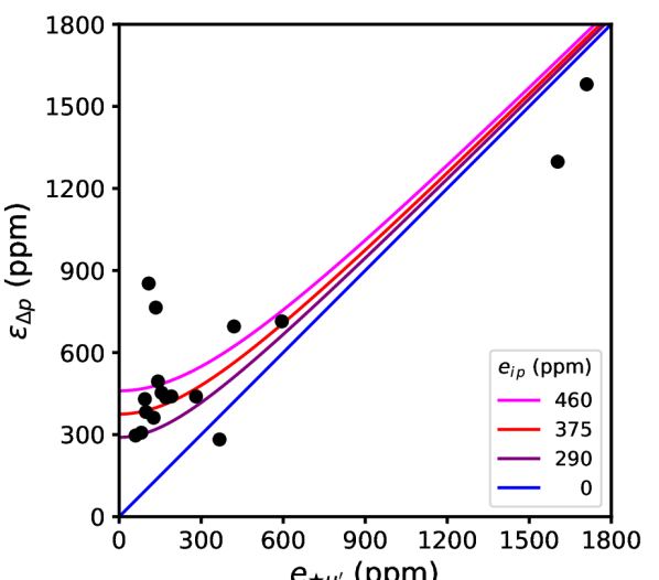
Table 4 also reports the unweighted standard deviation in compared to the mean, and the mean measured error, . If there are no further contributions to the error in polarization, , then the scatter in attributed to unaccounted for noise sources, represents the stellar variability in , i.e. or equivalently if we rotate the reference frame in the same way as first done in Sec. 4.2 (i.e. this is the counter-part to column 18 in Table 3). In Figure 4 we have plotted against . Owing to the large interstellar polarizations of these stars, whether or is larger, should be purely a matter of chance. We would therefore expect an equal number of points to fall either side of the blue line if is dominated by . This is clearly not the case, so there is an additional instrumental error, , that contributes to that needs to quantified, i.e.
| (18) |
Many more points are above the blue line in Fig. 4 at low values of , so a fixed error is more appropriate than one that scales with . In re-calibrating the modulators (Appendix C.4), we found a typical disagreement between and of 460 ppm. Using this figure overestimates the error (magenta line in Fig. 4) because it incorporates inaccuracies in the literature values of into the metric. If instead we take the median difference to the mean value of for each star, the result is 290 ppm for the observations in Table 4 and 155 ppm for the Pindari observations. The fact the precision is better in for the Pindari observations, which used only a small telescope but a single instrument/telescope set-up, is evidence that variation in instrument and set-up is the dominant source of the extra error. The purple line in Fig. 4 represents 280 ppm of added error; this appears to be an underestimate – too many points fall above the line, probably as a consequence of taking the mean from small datasets with uneven temporal sampling. The red line in the same figure is the intermediate value of 375 ppm, which more evenly divides the points, and which we adopt as 111111Adopting this value is still consistent with an assumption of Gaussian behaviour in both and , since 500 for all observations..
Having established a value for , we can now calculate error-weighted figures for and to determine the significance of the result, this is given in the final column of Table 4. Two stars are found to be variable at 3 sigma significance in ; both are also 3 significant variables in . Another four stars are 2 significant; two of these are not similarly significant in : HD 154445 and HD 161056; they both have early B spectral types. HD 111613 is a 3 significant variable in , but does not approach this level of significance in .
4.5 Variability time series
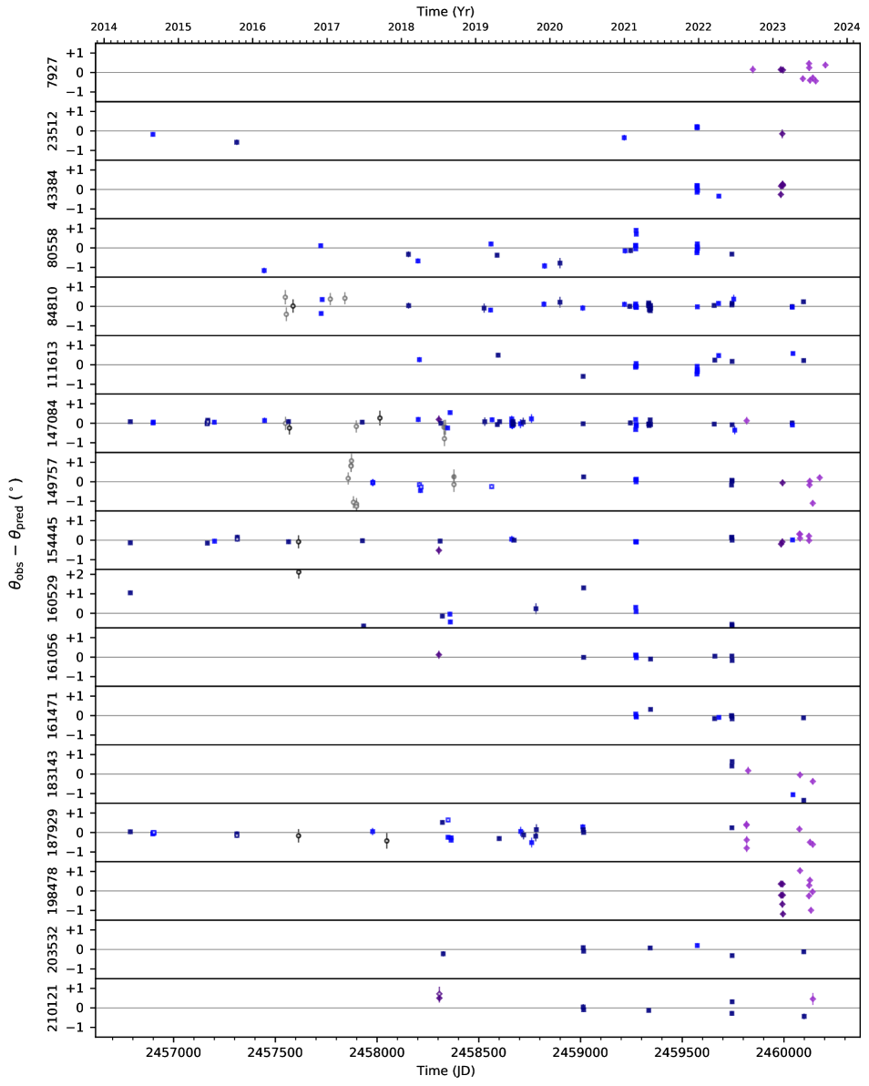
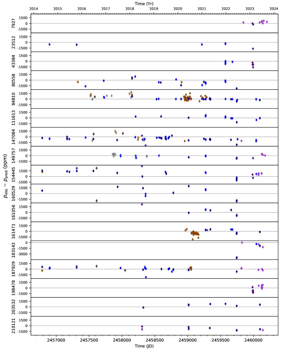
Here we present the and data for each star as a time series in Figs. 5 and 6, respectively. The latter includes data from the Pindari observatory, whereas the former does not, but otherwise excludes any point not on the first plot. Both figures include not just the data from runs with multiple stars observed, as used in Sec’s 4.2 and 4.3, but also Clear data (open symbols), and and Clear data which were re-calibrated based on Clear observations (where there are insufficient standard observation for the run). The additional data may be less accurate but is useful to fill in gaps in the time series (e.g. the 2016 HD 160529 datum). We have colour coded the observations by run as described in the caption. This is important because despite our precautions it is still a more precise matter to compare observations made within the same run. The error bars incorporate the error in , but if comparing observations intra-run the uncertainty is less than this.
Long term trends, or regular periodicity – where sufficiently sampled – would be revealed in Figs. 5 and 6, but neither behaviour is obvious. Considering both Figs. 5 and 6, the timescales of variability in and mostly appear correlated. For instance, the fast variability of HD 198478 is very easy to see within a run. Whereas the slower, but no less pronounced, variability seen in HD 160529 or HD 80558 occurs on longer timescales.
A noteworthy discrepancy is seen in Fig. 6 when comparing data from two early 2018 runs for HD 154445 – this is the only abrupt change in polarization observed for this star and is most likely not real. The Gemini North run (2018JUN) has the least reliable calibration, and this represents the first of these data points. Closer inspection reveals that all four observations from this run appear over-polarized. If we remove these points from the analysis in Sec. 4.4 (see below the mid-rule in Table 4) then the significance of variability in for both HD 154445 and HD 161056 falls below 2-, and so we regard neither as a variability candidate.
5 Discussion
5.1 Changes in over decades?
Four stars have refined values (column 11 in Table 3) significantly different to the literature using the criteria : HD 149757, HD 161056, HD 203532 and HD 210121 (other differences might be ascribed to stellar variability). This could indicate a slow change in over many decades. However, inspection of Fig. 5 does not support this notion. The data for these four stars do not hint at a long term trend despite spanning 4 years or more. If there is one it must only be apparent on longer time scales.
We sourced from only Bagnulo et al. (2017) for two stars: HD 161056 and HD 210121. HD 203532, includes data from Bagnulo et al. (2017) and Serkowski et al. (1975). Together, these are three of the five stars where was sourced from Bagnulo et al. (2017) (another star sourced from Bagnulo et al. (2017) is HD 80558, it has a large value, but is apparently also more variable). This is curious, because Bagnulo et al. (2017) is our most recent reference source, leading us to discount a slow drift in over time. Of the stars mentioned, three were observed by Bagnulo et al. in 2015 and have large negative values, HD 161056 was observed later in 2017 and has a large positive value. We conclude the difference is probably due to inaccurate calibration with FORS2 on the VLT.
This leaves HD 149757 as the only star of interest; for it we sourced from Serkowski et al. (1975), modified for with data from Wolff et al. (1996) to give 127.2∘. Our determination is almost 1∘ below this. The spectropolarimetry of Wolff et al. (1996) produces a figure of 125∘ for the band, while that of Wolstencroft & Smith (1984) gives 126∘. band observations described by McDavid (2000) range from to ; this seems like a lot of variation but it is not too different to that reported for other standards in McDavid (2000)’s agglomerated tables. Fig. 5 shows that few, if any, of these stars are really variable in over such a range.
More tellingly, perhaps, is the difference in behaviour between Wolff et al. (1996) and Wolstencroft & Smith (1984) – the slope is completely opposite in the two cases. This may point to intrinsic polarization that is episodic in nature. This would be in keeping with the irregular variability of the star’s photometry and spectroscopy (see Sec. 2.8). If so, it is not captured by the observations we analysed, we can assign only 0.211∘ to stellar variability. However, there is some evidence for a more active era early in 2017 in Clear observations made with Mini-HIPPI at the UNSW observatory – these can be seen to range over in Fig. 5.
5.2 Variability in compared to the literature
5.2.1 Literature data
In Fig. 7 we compare our determinations of intrinsic stellar variability to those available in the literature. As noted by Naghizadeh-Khouei (1991) only partial data is presented in some of these sources, and others make only a handful of measurements. Since there are so few determinations available, we employ very relaxed criteria to include as many comparisons as possible.
The core of the literature determinations presented come from Bastien et al. (1988) who derived variability in from the standard deviation of and ( comparable to our ) and compared that to the average error, (equivalent to our ). Their data includes typically tens of observations per star agglomerated from half a dozen different sources that made use of one of two of the better instruments available between 1983 and 1986.
Hsu & Breger (1982) present only representative data. They describe the data in detail, but do so in inconsistent ways that are not conducive to analysis. They actually observed each star tens of times between 1979 and 1981 (Breger & Hsu, 1982), but this is lost to us. All we have been able to do is digitise the data they plotted in their Fig. 1 and 2. We take their typical reported error of 0.1∘ as representative of and calculate the standard deviation of the presented data to derive . The data in their Fig. 1 represents a single 6 night observing run from August of 1981, Fig. 2 adds observations from 4 nights in September of the same year. We neglect the band data available for one target and use only the band observations.
Dolan & Tapia (1986) observed three of the same stars we did. They were mostly concerned with but in their Table 1 they present an average from all bands for 5 observations of HD 7927 from 1984, 3 of HD 111613 from 1980 and 1984, and 8 of HD 183143 from 1980 and 1984. We calculate standard deviations from this data. They report that their standard error is 0.09∘ based on a test from injecting a polarized signal into their system.
From Wiktorowicz et al. (2023) we take the band data for 3 stars, including HD 154445 which has only 3 observations; the others between 6 and 13. All the data sets span many years. Two data sets, from two different telescopes, are presented for HD 149757, we have plotted both. They give what is effectively directly in their Table 17, and we calculate from their and values in their Table 18 using Bastien et al. (1988)’s formula.
The variability of HD 43384 has been much discussed (see Sec. 2.3), we have two sources of data for HD 43384. Coyne (1972) presented data from 1969 to 1971 in two bandpasses, we take a high () subset of the more extensive dataset ( band) which then totals 9 observations; is only reported to the nearest degree, and so we add an additional 0.5∘ RMS error. Matsumura et al. (1997) made 17 observations relative to HD 21291121212Also claimed variable by Dolan & Tapia (1986) on the basis of complex and by comparison with Wolf (1972). with a single instrument with a typical error of 0.4∘ between 1991 and 1996. In the paper these data are plotted against phase assuming a 13.70 day period, with a sine curve fit. We digitised the points and calculated the standard deviation.
Finally, the values for one point for HD 149757 comes from McDavid (2000), who reports an insignificant variability based on agglomerated data from 1949 to 1996; the figures we have used come from the “Grand Average” of multi-band data in their Table 11 (though all the bands are pretty similar).
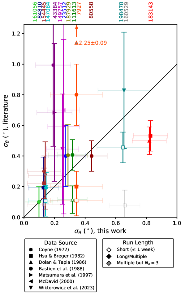
5.2.2 Comparison
The picture that emerges from Fig. 7 is one of surprisingly little disagreement. In particular Bastien et al. (1988)’s determinations are quite a good match for ours; with the only notably discrepant point being HD 7927. There are actually four literature determinations of HD 7927’s variability, and they disagree wildly. Our data on this target spans only a year. So, if the different estimates are to be reconciled it can only be through an appeal to episodic behaviour.
More broadly, it can be seen that variability determinations made from very short observing runs (open symbols in Fig. 7) yield low values (the exception is HD 198478 which exhibits obvious variability within a few nights). Amongst such determinations, we find good agreement with HD 147084 and HD 154445 which are two of the least variable stars in . In every other case there is disagreement with our data that spans years.
We do find agreement, largely within 1-, with almost everything that has been observed over a longer period. The biggest disagreements, still within 2-, are for HD 43384 which has some of the largest literature uncertainties, and HD 183143 for which we have only 7 observations over a year’s duration.
Despite the misgivings expressed by Clarke & Naghizadeh-Khouei (1994) and Naghizadeh-Khouei (1991), our analysis is consistent with the findings of earlier authors that many standards are in fact variable. A casual perusal of stellar polarimetry papers from the last 40 years will reveal that observers have largely ignored these reports of variability. This is partly because bright high polarization stars are not that common and alternative calibration methods not readily available. Therefore, the point is not to be able to declare a star variable or not based on statistical criteria, since this will not help observers much. There is enough evidence to suggest variability is common that we should consider it so. Yet, without quantification, this is an equally unhelpful statement. Any departure from spherical symmetry will produce a polarized signal, so it is a truism to write that everything is a polarimetric variable. The important question then is not which standards are variable? but rather what uncertainty should we ascribe to our measurements when using these standards? Our contention is that a careful analysis will assume the best estimate available, even if it is smaller than the formal detection threshold.
5.3 Astrophysical inferences
The data presented in this paper represents a rare opportunity to study the long-term small-scale polarimetric variability of high polarization stars with precision. In Table 6 – broken down as early-type supergiants, late-type supergiants, and other stars; and ordered by spectral type – the values of and are tabulated; The final column combines the two figures in a variability metric,
| (19) |
The groupings reveal B/A-type supergiants to be more variable as a category than either the F/G-type supergiants or the stars of other classes. In Figures 5 and 6 time series data is plotted, by star, in and , which we use along with the table and the QU diagrams in Fig. 3 to elucidate the nature of the variability below.
A thorough review of the QU patterns associated with different polarigenic mechanisms is given by Clarke (2010). In brief, periodic mechanisms, relating to binarity or persistent surface features – like magnetic spots – will be revealed by loops or figure-of-eight-type patterns. Polarization associated with a Be mechanism – material ejected from the equator followed by slow decretion from a disk – which has a preferred orientation, will fall predominantly along a straight ‘intrinsic line’. Polarization generated by randomly distributed clumps of gas within a (perhaps irregularly driven) stellar wind will manifest as a scatter plot. Whereas, an interstellar polarization drift would probably look like a random walk, but predominantly in .
| Standard | SpT | GCVS | |||
| (HD) | (ppm) | (ppm) | (ppm) | ||
| B/A-supergiants | |||||
| 198478 | B3 Ia | 644 | 595 | 877 | Cyg |
| 43384 | B3 Iab | 260 | 171 | 311 | Cyg |
| 80558 | B6 Ib | 604 | 420 | 736 | Cyg |
| 183143 | B7 Iae | 1673 | 1710 | 2392 | Cyg: |
| 111613 | A1 Ia | 256 | 281 | 380 | Cyg: |
| 160529 | A2 Ia | 1332 | 1604 | 2085 | Cyg |
| Mean | 1130 | ||||
| F/G-supergiants | |||||
| 7927 | F0 Ia | 0 | 367 | 367 | |
| 161471 | F2 Ia | 401 | 94 | 412 | |
| 187929 | F6 Ib | 275 | 142 | 309 | Cep |
| 84810 | G5 Iab | 0 | 60 | 60 | Cep |
| Mean | 287 | ||||
| Other classes | |||||
| 149757 | O9.5 Vn | 129 | 98 | 162 | Cas |
| 154445 | B1 V | 568 | 134 | 584 | |
| 161056 | B1.5 V | 569 | 108 | 579 | |
| 203532 | B3 IV | 0 | 81 | 81 | |
| 210121 | B7 II | 0 | 126 | 126 | |
| 23512 | A0 V | 274 | 191 | 334 | |
| 147084 | A4 II | 244 | 155 | 289 | |
| Mean | 308 | ||||
Notes – GN run (2018JUN) excluded from .
5.3.1 Cyg variables
Coyne (1972) was the first to (statistically) study the polarimetric variability of supergiant stars; which he found twice as variable as his control group. Together Fig. 3 and Table 6 are quite revealing in showing that it is the B/A-type supergiants – which are all Cyg variables – that are clearly more variable as a class, with all but one being formally 3- detected polarimetric variables. By and large their QU diagrams show no favoured direction nor clear pattern, something generally associated with a clumpy stellar wind mechanism (see refs. within Bailey et al., 2023).
In the era of space-photometry many early-type supergiants have been classified as Cyg variables on evidence of what is sometimes called stochastic low-frequency variability. In the GCVS catalog Cyg variables were originally classified as A- or B-type supergiants that displayed semi-regular radial velocity (RV) variability, said to be associated with the beating of many long period non-radial pulsations (Samus’ et al., 2017). Often, it is only assumed that the photometric and RV variability are associated. Nevertheless, many such stars are also known polarimetric variables, including for instance Cep (Hayes, 1975), Ori (Vitrichenko & Efimov, 1965), Rigel (Hayes, 1986) and Deneb itself (Cotton et al., 2024).
HD 80558, HD 111613, HD 183143, HD 183143: All four of these stars have past claims of variability. HD 183143 and HD 198478 were found to be variable in position angle by Hsu & Breger (1982). HD 183143 and HD 198478 are among the most clearly variable stars in our data; they have values of larger than 0.5∘. Dolan & Tapia (1986) later reported that HD 111613 and HD 183143 were variable in both and . HD 183143 shows perhaps the most dramatic shift in polarization we observed, and we also find it variable in . It is not surprising that it should be a polarimetric variable given the noteworthy emission in its spectral lines. It exhibits P Cygni profiles in Hα-δ indicative of a strong wind, that if clumped would be an asymmetric scattering medium. Bastien et al. (1988) reaffirmed HD 111613 and added HD 80558 as Cyg stars that were polarimetric variables. Clarke & Naghizadeh-Khouei (1994) criticised Bastien et al. (1988) but nevertheless agreed that HD 111613 was a polarimetric variable. We find HD 80558 to be variable at 3- significance in – easily seen in Fig. 3 – corresponding to an intrinsic variability of almost 0.4∘ – and almost 2- in . Thus, it seems the variability of these four stars is persistent.
HD 43384 has broad past evidence for variability (see Sec. 2.3). In particular, it was found to be variable in by Hsu & Breger (1982). However, it has the lowest value of of any of the six early-type supergiants we observed, and is the only one for which there is no formal variability detection. Matsumura et al. (1997) claim the star’s variability is periodic, but our data represent poor phase coverage for testing the reported period. So this is a potential cause of the disagreement. However, since we have just over a year’s data on this star, it is also possible this is simply insufficient for capturing episodic variability.
HD 160529 is the only B/A-supergiant without a prior variability claim; it is invariable in the short-run data presented by Hsu & Breger (1982). Repeat observations we made of the star in the same run also agree well. However, we see very large changes in and over years. Deneb, which is of the same spectral class and type, also exhibits polarimetric variability only on longer timescales than other Cyg variables (Cotton et al., 2024). As an LBV star, HD 160529 is undergoing mass loss that varies on a range of timescales associated with winds, pulsation and rotation (Stahl et al., 2003). As such, it is rather surprising that it has not previously been noted as a polarimetric variable. Another LBV star, P Cygni, has recently been the subject of a decade of spectropolarimetric study by Gootkin et al. (2020), who find that it displays a variety of polarimetric behaviour, in part associated with free-electron scattering off of clumps (mostly) uniformly distributed around the star. We deduce that the large polarimetric variability we see here in HD 160529 – amounting to 0.21 per cent; 0.64∘ – is associated with similar phenomena. Mass-loss from these stars is greatest during outburst. For HD 160529 this corresponds to an increase in temperature of 4000 K and a size increase of 180 . This process can take a number of years, consistent with the slow variation seen in Fig. 5 and Fig. 6.
Hayes (1984) made studies of the two early type Cyg stars Cam (O9.5 Ia) and Cas (B1 Ia). These two stars show both slow long term variability and faster short term variability in their polarization, in much the same way as do those early-type supergiants observed here with sufficient regularity. For instance, slow longer term variability is evident in HD 80558, faster short-term variability can be seen in both HD 80558 and HD 198478. We have not sampled all the B-type supergiants sufficiently on both timescales to test that these behaviours are simultaneously displayed, nonetheless it is a fair hypothesis. Hsu & Breger (1982) found early-type supergiants more variable on short time-scales than other standards and recommended against their use as such on that basis. Hayes (1984) concluded that the polarization variations he saw were the result of varying mass-loss in the stellar extended atmospheres and that he was witnessing the “waxing and waning of non-periodic clumpiness in the envelope,” such as to explain the variability at both timescales.
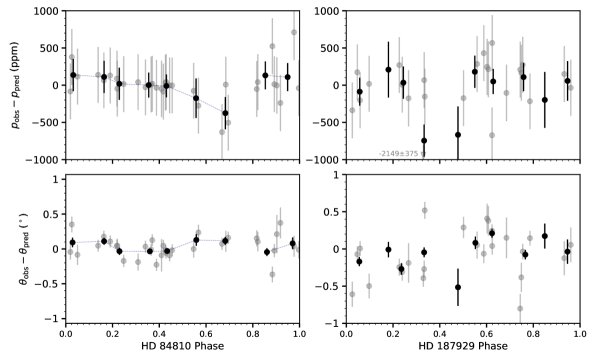
That similar polarimetric behaviour might be universal in early-type supergiants is suggested by Hayes (1986) similar findings regarding polarimetric variability in the later type (B8 Iae) Rigel. There, the variability was slower and the conclusion was that it resulted from localised disturbances in the stellar envelope originating at or below the photosphere. Cotton et al. (2024) recently observed analogous behaviour for (A2 Ia) Deneb and came to similar conclusions. The variability of (A2 Ia) HD 111613 seen by Bastien et al. (1988) is clearly slow in the same way, as is that we see in (A2 Ia) HD 160529. Together these data present a picture where the timescale of polarimetric variability in Cyg stars varies with spectral type. Given the contention that non-radial pulsations might be responsible for RV and photometric variability in similar stars (Bowman et al., 2019) and the associated debate about the plausibility of that hypothesis (Lenoir-Craig et al., 2022), we suggest that the time is right to examine the polarimetric variability of early-type supergiants as a class with a view to informing this question.
5.3.2 Suspected variables
Our observations of little intrinsic polarization amongst the F/G-supergiants is in keeping with expectations based on their cooler photospheres, which are less ionized, and produce less prominent winds. The standards of the other classes are of earlier types, but overall their variability is similar. There are no formal 3- detections of polarization variability amongst any of these other stars. However, the levels of variability we record are generally a match for Bastien et al. (1988)’s findings, and four stars show 2- detections; these might therefore be regarded as suspected variables. We briefly comment on each of these below:
HD 7927: We have already briefly discussed HD 7927 in Sec. 5.2. Bastien et al. (1988) found a greater variability for this star than we record, Hsu & Breger (1982)’s presented data gives a lower value. Bastien et al. (1988) also found the star to be significantly variable in , however we do not – our average error is about double theirs, though this does not wholly account for the discrepancy. It seems likely the star’s behaviour is episodic. Being of spectral type F0 Ia it does not meet the formal definition for an Cyg classification, though it is adjacent. As noted in Sec. 2.1 it displays the characteristics associated with the class, namely irregular RV and stochastic photometric variability, albeit at a low level. If the star does belong to the same class of objects then its polarimetric variability profile looks more like Rigel’s in Hayes (1986) than the earlier type supergiants studied in Hayes (1978, 1984).
HD 23512: Variability in for HD 23512 is 2- significant, corresponding to 0.256∘ – with which Bastien et al. (1988)’s results are consistent. This is surprising since as an ordinary A0 V star it should be one of the least intrinsically polarized (Cotton et al., 2016), a fact already alluded to by Hall (1951)131313At this time HD 23512 was the closest star with a polarization detection.. This suggests that its companion may be a polarimetric variable. The companion is responsible for 16 per cent of the combined flux, but being of small separation and discovered by Lunar occultation141414It should be noted that the discovery is relatively recent. Earlier occultation studies did not find a companion (references within Guthrie, 1987)., little else is known about it. Breger (1984) confirmed Hall (1951)’s initial finding that HD 23512 is much more polarized than any of the other bright stars in the cluster, but showed its wavelength dependence was typical. This leads us to speculate that the companion might instead be a bright background star. As discussed by Guthrie (1987), HD 23512 is unusual in other ways: it displays anomalously weak absorption at 2200 Å and in several other bands for a star of its spectral type, and is depleted in calcium. These factors may provide some clues as to the nature of the other star. If the ‘B’ component is predominantly responsible for the polarization variability, the scale of it would be 2000 ppm, which is not unreasonable for a supergiant or a Be star.
HD 187929: Bastien et al. (1988) describe variability consistent with our measurements. The star has a magnetic field detection, but it is too small to produce significant linear broadband polarization (Barron et al., 2022). Classically, Cep variables (Cepheids) should not be polarimetric variables as radial pulsations produce no net polarization change (Odell, 1979). However, Polyakova & Sudakov (1981) and Polyakova (1984, 1987, 1990) claim to have measured phase-dependant polarization that is bound by a three-lobed “rosette” in the QU diagrams of many such stars. Polyakova & Sudakov (1981) ascribe this to an artefact of calibration owing to broadband measurements of colour-variable objects, but Polyakova (1990) later suggested an intrinsic polarization mechanism due to a circumstellar envelope 20-30 per cent larger at the equator than the pole – Kervella et al. (2006) thought this worthy of investigation.
We plotted the and against phase for both Cep variables in Fig. 8, since nothing was obvious from the QU diagrams in Fig. 3. Surprisingly, there is a hint of phase dependant behaviour in the binned data of HD 84810 consistent with that described in the literature, albeit well below our formal detection thresholds – investigating this is beyond the scope of the paper. There is no clear phase-dependant behaviour for HD 187929; therefore, we discard the two aforementioned hypotheses as variable polarization mechanisms for it. Another possibility involves the star’s binarity. The unseen B9.8 V companion (Evans, 1991) has an unknown orbit. Both a long period orbit and one as short as 55 d that is face-on are viable based on current data (Benedict et al., 2022). A truly face-on orbit would result in a rotation of with no change in . Detailed calculations are required to determine if either photospheric reflection or entrained gas are good hypotheses in this case, though even a 55 d period seems like it would not produce a lot of polarization. If it does, further observations could reveal the geometry of the orbit (Brown et al., 1978; Cotton et al., 2020).
HD 210121: The final star displaying a variability more significant than 2- is HD 210121 – 0.264∘. This star has one of the smallest values, so this corresponds to an of only 126 ppm. If the star really is a bright giant, winds might be responsible. However, this polarization is small enough that many mechanisms could explain such variability. Any of non-radial pulsations, a binary mechanism, emission behaviour, or interstellar drift could be responsible, but no clear leads present themselves in the literature.
| Correction Removed | ||
| (∘) | (∘) | |
| Precession (original equinox) | 0.229 | 0.396 |
| New * | 0.112 | 0.796 |
| ( to ) | 0.021 | 0.331 |
| Weighting | 0.011 | 0.510 |
| Precession (2020 equinox) | 0.005 | 0.035 |
| (airmass) | 0.004 | 0.078 |
| Faraday Rotation | 0.002 | 0.007 |
| All | 0.312 | 1.030 |
Notes – * Uses literature values for as per Table 9.
5.4 Relative impact of corrections
In Sec’s 3.1 and 4 we have carried out a series of corrections aimed at more accurately calibrating the telescope position angle for each run. In table 7 we rank each correction by the median difference between our final determination, and what we’d get neglecting the specified corrections. For this we include all except the Pindari runs.
Assuming the new values of reported are the real values, the typical improvement in determination is 0.3∘. The most significant corrections are due to precession and the re-determined values. Here we have calculated for each star in a 2020 equinox. Our observations span a decade, from 2014 to 2023. It can be seen that making precession corrections is now essential to achieve 0.1∘ accuracy if working from older literature. However, using contemporary sources will be suitable for most applications.
The largest values for (airmass) correspond to runs with Clear rather than observations. For instruments where rotates with wavelength, narrower bands are better for calibration. If one wants to simplify their reduction routine, this analysis suggests they need not worry about wavelength correction post-fact to account for airmass, but it is a good idea to make band corrections before beginning if the literature data is in a different filter.
Applying the weightings associated with , , and is only important in a few cases – those where only a few standard measurements were obtained and one of them was one of the most variable stars. If one observes only the least variable standards, then weighting will generally not be needed. However, if forced to use less reliable standards, one should use the best weightings available, and observe as many different standards as possible – since a standard variable on long timescales may be invariable on short ones and because scales .
5.5 Recommendations for observers
| Standard | ||||
| (HD) | (∘) | (∘) | () | () |
| 7927 | 93.165 | 0.321 | 5.7 | 0.4 |
| 23512 | 30.706 | 0.256 | 3.6 | 0.5 |
| 43384 | 170.295 | 0.167 | 2.6 | 0.6 |
| 80558 | 162.512 | 0.384 | 1.4 | 0.6 |
| 84810 | 99.997 | 0.110 | 0.0 | 0.7 |
| 111613 | 80.836 | 0.266 | 0.0 | 0.2 |
| 147084 | 32.028 | 0.118 | 0.0 | 0.6 |
| 149757 | 126.218 | 0.211 | 5.0 | 0.5 |
| 154445 | 89.985 | 0.110 | 0.0 | 0.5 |
| 160529 | 18.748 | 0.640 | 3.5 | 0.7 |
| 161056 | 68.034 | 0.082 | 1.5 | 0.6 |
| 161471 | 2.087 | 0.123 | 1.1 | 0.7 |
| 183143 | 179.299 | 0.819 | 0.0 | 0.5 |
| 187929 | 93.703 | 0.241 | 7.3 | 0.5 |
| 198478 | 2.417 | 0.628 | 0.0 | 0.6 |
| 203532 | 124.360 | 0.175 | 2.4 | 2.7 |
| 210121 | 153.903 | 0.264 | 8.6 | 0.3 |
Notes – Values of are given for a 2020 equinox. Here the band nominally corresponds to 470 nm. The best standards are backed in gray.
We reiterate the best determinations for position angle parameters in Table 8, as they are important for our recommendations to observers seeking better position angle calibration. Both and its associated variability are derived in Sec. 4.3, the other parameters come from the literature as described in Appendix A. Using this data and applying the advice below will allow for better than 0.1∘ error in from a handful of observations in most circumstances. In order of importance our recommendations are:
- 1.
-
2.
Use the best available determination of for your standards, report the value assigned and provenance of the standards employed. Ideally all determinations should be made with the same . For the stars studied here, we recommend the values in Table 8. If other standards are needed, we prefer the values given in Hsu & Breger (1982), and then, if those are unavailable, determinations tied to Serkowski et al. (1975)’s calibration and determined from long run data.
-
3.
Use the available information in determining for your bandpass. In many cases a full bandpass model will not be required, but if carrying out one for this purpose, use the spectral types and values of , , , , and given in Table 1 for the stars studied here, or follow the methodologies laid out in Appendix B to determine values for others.
-
4.
Characterise the position angle error associated with your instrument independent of photon shot noise. To achieve this, one should observe at least one, preferably a few, of the least variable standards multiple times within a few nights, calculate the standard deviation of each, subtract the RMS shot-noise contributions, and take the median. Such a determination should be made and reported as part of commissioning an instrument on a new telescope. Without this information combining data between groups or even just runs to a high precision in is fraught.
-
5.
Choose the most reliable standards available based on reported variability. For the stars studied here, we recommend the values in Table 8. For other standards, taking from Bastien et al. (1988) is recommended. Where of a potential standard is unknown, the following equation might be used as a first approximation:
(20) where is in degrees, is the interstellar component of the polarization (equal to for an ideal standard), and should be taken as 1130 ppm for an Cyg variable, and 300 ppm otherwise, on the basis of the means in Table 6.
-
6.
Especially where the available standards might be less reliable, observe multiple standards (ideally ) for calibration and weight the result according to the RMS sum of measurement uncertainty and the best estimate of variability.
6 Conclusions
Long duration studies of high polarization stars are rare leading us to explore the astrophysical implications of our findings: Extreme stars are extremely polarized. The most polarized object in our study, the LBV star HD 160529, is found to also be one of the largest amplitude polarimetric variables. This star has not previously been noted as a polarimetric variable, seemingly it is variable only on longer timescales.
Large amplitude polarization variability is common and shows no preferred orientation in Cygni variables (HD 80558, HD 111613, HD 183143, HD 198478), a behaviour that may extend to the F0 Ia HD 7927 at lower levels. By analogy with historical studies, clumpy winds are the most likely polarigenic mechanism, but pulsation might also play a role and a dedicated observational program and investigation is recommended.
Later type supergiants and other ordinary stars that happen to be extremely reddened make more reliable standards. The best standards are HD 84810, HD 147084, HD 154445, HD 161056 and HD 161471, for which we attribute variability . However, polarization variability may also be present, at lower levels, where we make 2- detections. There is also evidence for variability in the literature or extended data for other stars in our sample (i.e. HD 43384 and HD 149757). The data analysed might be too thin to capture episodic behaviour in these cases; Hayes (1975) came to a similar conclusion after finding no variability for HD 149757.
The companion to HD 23512 may be a large amplitude polarimetric variable. HD 187929 displays position angle variability not correlated with the Cepheid phase, an observation that favours a companion in a face-on orbit.
Our results largely vindicate the findings of Bastien et al. (1988) who were criticised for a lack of statistical rigor by Clarke & Naghizadeh-Khouei (1994) in combining data from multiple sources. The methodology we apply alleviates the problems associated with combining data from disparate observing runs. Key to this is the application of a Co-ordinate Difference Matrix which works by amalgamating difference measurements of pairs of points.
By combining a decade’s worth of data we have been able to make more accurate and precise determinations of , as well as estimates of its variability, which are tabulated in Table 8. The other standard properties, as given in Tables 8 and 1, have been derived from literature we have curated to minimise the impacts of disagreement between different researchers; these should also be adopted. Along with these improvements, which are quantitatively assessed in Sec. 5.4, we provide specific recommendations for observers in Sec. 5.5 that will allow for better than 0.1∘ calibration in telescope position angle from a handful of observations in most circumstances.
Acknowledgements
This research has made use of the SIMBAD database, operated at CDS, Strasbourg, France; NASA’s Astrophysics Data System; and the VizieR catalogue access tool, CDS, Strasbourg, France (\doi10.26093/cds/vizier). Based on spectral data retrieved from the ELODIE archive at Observatoire de Haute-Provence (OHP). We acknowledge with thanks the variable star observations from the AAVSO International Database contributed by observers worldwide and used in this research.
JPM acknowledges support by the National Science and Technology Council of Taiwan under grant NSTC 112-2112-M-001-032-MY3. Funding for the construction of HIPPI-2 was provided by UNSW through the Science Faculty Research Grants Program. We thank the Friends of MIRA for their support.
We thank the former Director of the Australian Astronomical Observatory, Prof. Warrick Couch, the current Director of Siding Spring Observatory, Prof. Chris Lidman, and all of the staff at the AAT for their support of the HIPPI and HIPPI-2 projects. We thank Prof. Miroslav Filipovic for providing access to the Penrith Observatory. We thank all of the additional student volunteers at UNSW, MIRA, WSU and elsewhere, who assisted with observations at the various observatories. We thank Dr. Wm. Bruce Weaver for useful comments on the manuscript. We thank Dr. Sarbani Basu for help acquiring a reference.
Based in part on data obtained at Siding Spring Observatory. We acknowledge the traditional owners of the land on which the AAT stands, the Gamilaraay people, and pay our respects to elders past and present.
Based in part on data obtained at Western Sydney University, Penrith Observatory. We acknowledge the traditional owners of the land on which the WSU Penrith Observatory stands, the Dharug people, and pay our respects to elders past and present.
Data Availability
All of the data for this work is available in a catalogue described in Section 3.
References
- Abt & Levato (1978) Abt H. A., Levato H., 1978, PASP, 90, 201
- Abt et al. (1965) Abt H. A., Barnes R. C., Biggs E. S., Osmer P. S., 1965, ApJ, 142, 1604
- Adams et al. (1924) Adams W. S., Joy A. H., Sanford R. F., 1924, PASP, 36, 137
- Aiello et al. (1988) Aiello S., Barsella B., Chlewicki G., Greenberg J. M., Patriarchi P., Perinotto M., 1988, A&AS, 73, 195
- Albrecht (1921) Albrecht S., 1921, ApJ, 54, 161
- Arellano Ferro et al. (1988) Arellano Ferro A., Parrao L., Giridhar S., 1988, PASP, 100, 993
- Baechler et al. (2020) Baechler G., Dübgen F., Golnoosh E., Krekovíc M., Martin V., 2020, SIAM J. Matrix Anal. Appl., 41, 332
- Bagnulo et al. (2017) Bagnulo S., et al., 2017, A&A, 608, A146
- Bailey & Hough (1982) Bailey J., Hough J. H., 1982, PASP, 94, 618
- Bailey et al. (2010) Bailey J., Lucas P. W., Hough J. H., 2010, MNRAS, 405, 2570
- Bailey et al. (2015) Bailey J., Kedziora-Chudczer L., Cotton D. V., Bott K., Hough J. H., Lucas P. W., 2015, MNRAS, 449, 3064
- Bailey et al. (2017) Bailey J., Cotton D. V., Kedziora-Chudczer L., 2017, MNRAS, 465, 1601
- Bailey et al. (2019) Bailey J., Cotton D. V., Kedziora-Chudczer L., De Horta A., Maybour D., 2019, Nature Astronomy, 3, 636
- Bailey et al. (2020) Bailey J., Cotton D. V., Kedziora-Chudczer L., De Horta A., Maybour D., 2020, Publ. Astron. Soc. Australia, 37, e004
- Bailey et al. (2021) Bailey J., et al., 2021, MNRAS, 502, 2331
- Bailey et al. (2023) Bailey J., Cotton D. V., De Horta A., Kedziora-Chudczer L., Shastri O., 2023, MNRAS, 520, 1938
- Bailey et al. (2024) Bailey J., Howarth I. D., Cotton D. V., Kedziora-Chudczer L., De Horta A., Martell S. L., Eldridge C., Luckas P., 2024, MNRAS, 529, 374
- Balona & Dziembowski (1999) Balona L. A., Dziembowski W. A., 1999, MNRAS, 309, 221
- Balona & Kambe (1999) Balona L. A., Kambe E., 1999, MNRAS, 308, 1117
- Barron et al. (2022) Barron J. A., Wade G. A., Evans N. R., Folsom C. P., Neilson H. R., 2022, MNRAS, 512, 4021
- Bastien et al. (1988) Bastien P., Drissen L., Menard F., Moffat A. F. J., Robert C., St-Louis N., 1988, AJ, 95, 900
- Bastien et al. (2007) Bastien P., Vernet E., Drissen L., Ménard F., Moffat A. F. J., Robert C., St-Louis N., 2007, in Sterken C., ed., Astronomical Society of the Pacific Conference Series Vol. 364, The Future of Photometric, Spectrophotometric and Polarimetric Standardization. p. 529
- Behr (1959) Behr A., 1959, PhD thesis, Univ. Gottingen (Germany)
- Benedict et al. (2007) Benedict G. F., et al., 2007, AJ, 133, 1810
- Benedict et al. (2022) Benedict G. F., Barnes T. G., Evans N. R., Cochran W. D., Anderson R. I., McArthur B. E., Harrison T. E., 2022, AJ, 163, 282
- Berdyugin et al. (1995) Berdyugin A., Snare M. O., Teerikorpi P., 1995, A&A, 294, 568
- Berdyugin et al. (2018) Berdyugin A., Piirola V., Sakanoi T., Kagitani M., Yoneda M., 2018, A&A, 611, A69
- Bersier (1996) Bersier D., 1996, A&A, 308, 514
- Blinov et al. (2023) Blinov D., et al., 2023, A&A, 677, A144
- Bohm-Vitense & Love (1994) Bohm-Vitense E., Love S. G., 1994, ApJ, 420, 401
- Borra et al. (1981) Borra E. F., Fletcher J. M., Poeckert R., 1981, ApJ, 247, 569
- Boss (1910) Boss L., 1910, Preliminary General Catalogue of 6188 stars for the epoch 1900
- Boss et al. (1936) Boss B., Albrecht S., Jenkins H., Raymond H., Roy A. J., Varnum W. B., Wilson R. E., Boss L., 1936, General catalogue of 33342 stars for the epoch 1950 …
- Bott et al. (2016) Bott K., Bailey J., Kedziora-Chudczer L., Cotton D. V., Lucas P. W., Marshall J. P., Hough J. H., 2016, MNRAS, 459, L109
- Bott et al. (2018) Bott K., Bailey J., Cotton D. V., Kedziora-Chudczer L., Marshall J. P., Meadows V. S., 2018, AJ, 156, 293
- Bott et al. (2022) Bott K., Bailey J., Kedziora-Chudczer L., Wiktorowicz S., Nofi L., Kane S., 2022, in Bulletin of the American Astronomical Society. p. 407.04
- Bowman et al. (2019) Bowman D. M., et al., 2019, Nature Astronomy, 3, 760
- Breger (1984) Breger M., 1984, A&A, 137, 145
- Breger & Hsu (1982) Breger M., Hsu J. C., 1982, Bulletin d’Information du Centre de Donnees Stellaires, 23, 51
- Brown et al. (1978) Brown J. C., McLean I. S., Emslie A. G., 1978, A&A, 68, 415
- Carciofi et al. (2007) Carciofi A. C., Magalhães A. M., Leister N. V., Bjorkman J. E., Levenhagen R. S., 2007, ApJ, 671, L49
- Cardelli et al. (1989) Cardelli J. A., Clayton G. C., Mathis J. S., 1989, ApJ, 345, 245
- Castelli & Kurucz (2003) Castelli F., Kurucz R. L., 2003, in Piskunov N., Weiss W. W., Gray D. F., eds, ESA Special Publication Vol. 210, Modelling of Stellar Atmospheres. p. A20 (arXiv:astro-ph/0405087)
- Chen et al. (2024) Chen J., Zhang R., Zhou Y., Jain R., Xu Z., Rossi R., Chen C., 2024, arXiv e-prints, p. arXiv:2402.04754
- Chentsov (2004) Chentsov E. L., 2004, Astronomy Letters, 30, 325
- Cholakyan (1986) Cholakyan V. G., 1986, Astrophysics, 25, 531
- Cikota et al. (2018) Cikota A., et al., 2018, A&A, 615, A42
- Clarke (2010) Clarke D., 2010, Stellar Polarimetry. Wiley-VCH Verlag GmbH & Co. KGaA, Weinheim.
- Clarke & Al-Roubaie (1983) Clarke D., Al-Roubaie A., 1983, MNRAS, 202, 173
- Clarke & Naghizadeh-Khouei (1994) Clarke D., Naghizadeh-Khouei J., 1994, AJ, 108, 687
- Clemens & Tapia (1990) Clemens D. P., Tapia S., 1990, PASP, 102, 179
- Cotton et al. (2016) Cotton D. V., Bailey J., Kedziora-Chudczer L., Bott K., Lucas P. W., Hough J. H., Marshall J. P., 2016, MNRAS, 455, 1607
- Cotton et al. (2017) Cotton D. V., Bailey J., Howarth I. D., Bott K., Kedziora-Chudczer L., Lucas P. W., Hough J. H., 2017, Nature Astronomy, 1, 690
- Cotton et al. (2019a) Cotton D. V., et al., 2019a, MNRAS, 483, 1574
- Cotton et al. (2019b) Cotton D. V., et al., 2019b, MNRAS, 483, 3636
- Cotton et al. (2020) Cotton D. V., Bailey J., Kedziora-Chudczer L., De Horta A., 2020, MNRAS, 497, 2175
- Cotton et al. (2022a) Cotton D. V., et al., 2022a, Nature Astronomy, 6, 154
- Cotton et al. (2022b) Cotton D. V., Bailey J., Larson J., Weaver W. B., Perkins J., Henderson G., 2022b, Research Notes of the American Astronomical Society, 6, 209
- Cotton et al. (2024) Cotton D. V., Bailey J., Perkins J., Buzasi D. L., Boiko I., 2024, arXiv e-prints, p. arXiv:2404.17707
- Cox et al. (2007) Cox N., et al., 2007, Astronomy & Astrophysics, 465, 899
- Cox et al. (2017) Cox N. L. J., et al., 2017, A&A, 606, A76
- Coyne (1972) Coyne G. V., 1972, in Hack M., ed., Colloquium on Supergiant Stars. Third Colloquium on Astrophysics held in Trieste. pp 93–107
- Coyne & Gehrels (1966) Coyne G. V., Gehrels T., 1966, AJ, 71, 355
- Coyne et al. (1974) Coyne G. V., Gehrels T., Serkowski K., 1974, AJ, 79, 581
- Danks & Dennefeld (1994) Danks A. C., Dennefeld M., 1994, PASP, 106, 382
- Dattorro (2005) Dattorro J., 2005, Convex optimization & Euclidean distance geometry. MeBoo Publishing, Palo Alto, California, U.S.A.
- Dolan & Tapia (1986) Dolan J. F., Tapia S., 1986, PASP, 98, 792
- Dyck & Jennings (1971) Dyck H. M., Jennings M. C., 1971, AJ, 76, 431
- Dyck & Jones (1978) Dyck H. M., Jones T. J., 1978, AJ, 83, 594
- Dyck et al. (1971) Dyck H. M., Forbes F. F., Shawl S. J., 1971, AJ, 76, 901
- ESA (1997) ESA ., 1997, VizieR Online Data Catalog, p. I/239
- Ebenbichler et al. (2022) Ebenbichler A., et al., 2022, A&A, 662, A81
- Eggen (1982) Eggen O. J., 1982, PASP, 94, 952
- Eggleton & Tokovinin (2008) Eggleton P. P., Tokovinin A. A., 2008, MNRAS, 389, 869
- Evans (1991) Evans N. R., 1991, ApJ, 372, 597
- Evans & Howarth (2003) Evans C. J., Howarth I. D., 2003, MNRAS, 345, 1223
- Evans et al. (2013) Evans N. E., Bond H. E., Schaefer G. H., Mason B. D., Karovska M., Tingle E., 2013, AJ, 146, 93
- Faraday (1846) Faraday M., 1846, The London, Edinburgh, and Dublin Philosophical Magazine and Journal of Science, 28, 294
- Finkel (1964) Finkel J., 1964, Journal of Atmospheric and Terrestrial Physics, 26, 297
- Fitzpatrick & Massa (2007) Fitzpatrick E. L., Massa D., 2007, ApJ, 663, 320
- Frisch et al. (2022) Frisch P. C., et al., 2022, ApJS, 259, 48
- Gehrels & Silvester (1965) Gehrels T., Silvester A. B., 1965, AJ, 70, 579
- Gootkin et al. (2020) Gootkin K., et al., 2020, ApJ, 900, 162
- Granes & Herman (1972) Granes P., Herman R., 1972, in Hack M., ed., Colloquium on Supergiant Stars. Third Colloquium on Astrophysics held in Trieste. pp 58–67
- Gray & Garrison (1989) Gray R. O., Garrison R. F., 1989, ApJS, 69, 301
- Gray et al. (2001) Gray R. O., Napier M. G., Winkler L. I., 2001, AJ, 121, 2148
- Grunhut et al. (2010) Grunhut J. H., Wade G. A., Hanes D. A., Alecian E., 2010, MNRAS, 408, 2290
- Guthrie (1987) Guthrie B. N. G., 1987, QJRAS, 28, 289
- Hall (1949) Hall J. S., 1949, Science, 109, 166
- Hall (1951) Hall J. S., 1951, AJ, 56, 40
- Hall & Mikesell (1950) Hall J. S., Mikesell A. H., 1950, Publications of the U.S. Naval Observatory Second Series, 17, 3
- Hayes (1975) Hayes D. P., 1975, ApJ, 197, L55
- Hayes (1978) Hayes D. P., 1978, ApJ, 219, 952
- Hayes (1984) Hayes D. P., 1984, AJ, 89, 1219
- Hayes (1986) Hayes D. P., 1986, ApJ, 302, 403
- Heckert & Filliben (2003) Heckert N. A., Filliben J. A., 2003, NIST Handbook 148: Dataplot Reference Manual, Volume 2: Let Subcommands and Library Functions. National Institute of Standards and Technology
- Hiltner (1949) Hiltner W. A., 1949, Science, 109, 165
- Hiltner (1951) Hiltner W. A., 1951, ApJ, 114, 241
- Hindsley & Bell (1989) Hindsley R. B., Bell R. A., 1989, ApJ, 341, 1004
- Hoag et al. (1961) Hoag A. A., Johnson H. L., Iriarte B., Mitchell R. I., Hallam K. L., Sharpless S., 1961, Publications of the U.S. Naval Observatory Second Series, 17, 344
- Hobbs (1979) Hobbs L. M., 1979, PASP, 91, 690
- Hough et al. (2006) Hough J. H., Lucas P. W., Bailey J. A., Tamura M., Hirst E., Harrison D., Bartholomew-Biggs M., 2006, PASP, 118, 1302
- Houk (1978) Houk N., 1978, Michigan Catalogue of Two-dimensional Spectral Types for the HD stars
- Houk (1982) Houk N., 1982, Michigan Catalogue of Two-dimensional Spectral Types for the HD stars. Volume 3. Declinations 40∘ to 26∘.
- Howarth et al. (2023) Howarth I. D., Bailey J., Cotton D. V., Kedziora-Chudczer L., 2023, MNRAS, 520, 1193
- Hsu & Breger (1982) Hsu J. C., Breger M., 1982, ApJ, 262, 732
- Hubrig et al. (2011) Hubrig S., Oskinova L. M., Schöller M., 2011, Astronomische Nachrichten, 332, 147
- Humphreys (1978) Humphreys R. M., 1978, ApJS, 38, 309
- Jurkić et al. (2011) Jurkić T., Sarta Deković M., Dominis Prester D., Kotnik-Karuza D., 2011, Astrophysics and Space Science, 335, 113
- Kemp (1972) Kemp J. C., 1972, ApJ, 175, L35
- Kervella et al. (2006) Kervella P., Mérand A., Perrin G., Coudé du Foresto V., 2006, A&A, 448, 623
- Kraus et al. (2015) Kraus M., et al., 2015, Astronomy & Astrophysics, 581, A75
- Krekovic (2020) Krekovic M., 2020, PhD thesis, EPFL, doi:10.5075/epfl-thesis-9840
- Krełowski et al. (2021) Krełowski J., Galazutdinov G. A., Gnaciński P., Hakalla R., Szajna W., Siebenmorgen R., 2021, MNRAS, 508, 4241
- Lallement et al. (2019) Lallement R., Babusiaux C., Vergely J. L., Katz D., Arenou F., Valette B., Hottier C., Capitanio L., 2019, A&A, 625, A135
- Larson et al. (1996) Larson K. A., Whittet D. C. B., Hough J. H., 1996, ApJ, 472, 755
- Larson et al. (2000) Larson K. A., Wolff M. J., Roberge W. G., Whittet D. C. B., He L., 2000, ApJ, 532, 1021
- Lenoir-Craig et al. (2022) Lenoir-Craig G., et al., 2022, ApJ, 925, 79
- Lesh (1968) Lesh J. R., 1968, ApJS, 17, 371
- Levato et al. (1987) Levato H., Malaroda S., Morrell N., Solivella G., 1987, ApJS, 64, 487
- Lewis et al. (2022) Lewis F., Bailey J., Cotton D. V., Howarth I. D., Kedziora-Chudczer L., van Leeuwen F., 2022, MNRAS, 513, 1129
- Liu et al. (1991) Liu T., Janes K. A., Bania T. M., 1991, ApJ, 377, 141
- Liu et al. (2023) Liu Y., Nie L., Dong R., Chen G., 2023, Proceedings of the Institution of Mechanical Engineers, Part C: Journal of Mechanical Engineering Science, 237, 4203
- Luck (2014) Luck R. E., 2014, AJ, 147, 137
- Lupie & Nordsieck (1987) Lupie O. L., Nordsieck K. H., 1987, AJ, 93, 214
- Lyot (1929) Lyot B., 1929, PhD thesis, Universite Pierre et Marie Curie (Paris VI), France
- Markowitz (1951) Markowitz W., 1951, AJ, 56, 134
- Marshall et al. (2016) Marshall J. P., et al., 2016, ApJ, 825, 124
- Marshall et al. (2020) Marshall J. P., Cotton D. V., Scicluna P., Bailey J., Kedziora-Chudczer L., Bott K., 2020, MNRAS, 499, 5915
- Marshall et al. (2023) Marshall J. P., Cotton D. V., Bott K., Bailey J., Kedziora-Chudczer L., Brown E. L., 2023, MNRAS, 522, 2777
- Martin et al. (1999) Martin P. G., Clayton G. C., Wolff M. J., 1999, ApJ, 510, 905
- Mason et al. (2001) Mason B. D., Wycoff G. L., Hartkopf W. I., Douglass G. G., Worley C. E., 2001, AJ, 122, 3466
- Mathewson & Ford (1970) Mathewson D. S., Ford V. L., 1970, Mem. RAS, 74, 139
- Matsumura et al. (1997) Matsumura M., Seki M., Kawabata K., 1997, in IAU Joint Discussion. p. 25
- McDavid (2000) McDavid D., 2000, AJ, 119, 352
- Merrill & Burwell (1933) Merrill P. W., Burwell C. G., 1933, ApJ, 78, 87
- Mozaffari et al. (2019) Mozaffari S., Akbarzadeh M., Vogel T., 2019, in Structures Congress 2019. pp 353–361, doi:10.1061/9780784482247.032
- Nagata (1990) Nagata T., 1990, ApJ, 348, L13
- Naghizadeh-Khouei (1991) Naghizadeh-Khouei J., 1991, Master’s thesis, University of Glasgow (United Kingdom), https://theses.gla.ac.uk/id/eprint/78264
- Nakamura et al. (2010) Nakamura K., Hamana Y., Ishigami Y., Matsui T., 2010, Nuclear Instruments and Methods in Physics Research A, 623, 276
- Negueruela et al. (2004) Negueruela I., Steele I. A., Bernabeu G., 2004, Astronomische Nachrichten, 325, 749
- O’Donnell (1994) O’Donnell J. E., 1994, ApJ, 422, 158
- Odell (1979) Odell A. P., 1979, PASP, 91, 326
- Percy (1989) Percy J. R., 1989, Information Bulletin on Variable Stars, 3353, 1
- Piccone & Kobulnicky (2022) Piccone A. N., Kobulnicky H. A., 2022, ApJ, 924, 138
- Pigott (1785) Pigott E., 1785, Philosophical Transactions of the Royal Society of London Series I, 75, 127
- Piirola et al. (2014) Piirola V., Berdyugin A., Berdyugina S., 2014, in Ramsay S. K., McLean I. S., Takami H., eds, Society of Photo-Optical Instrumentation Engineers (SPIE) Conference Series Vol. 9147, Ground-based and Airborne Instrumentation for Astronomy V. p. 91478I, doi:10.1117/12.2055923
- Piirola et al. (2020) Piirola V., et al., 2020, A&A, 635, A46
- Piirola et al. (2021) Piirola V., Kosenkov I. A., Berdyugin A. V., Berdyugina S. V., Poutanen J., 2021, AJ, 161, 20
- Plachinda (2000) Plachinda S. I., 2000, A&A, 360, 642
- Polyakova (1984) Polyakova T. A., 1984, Pisma v Astronomicheskii Zhurnal, 10, 749
- Polyakova (1987) Polyakova T. A., 1987, Astrofizika, 26, 469
- Polyakova (1990) Polyakova T. A., 1990, Pisma v Astronomicheskii Zhurnal, 16, 916
- Polyakova & Sudakov (1981) Polyakova T. A., Sudakov S. V., 1981, Prisma v Astronomicheskii Zhurnal, 7, 106
- Pourbaix et al. (2004) Pourbaix D., et al., 2004, A&A, 424, 727
- Rachford et al. (2009) Rachford B. L., et al., 2009, ApJS, 180, 125
- Reed (2003) Reed B. C., 2003, AJ, 125, 2531
- Rieke & Lebofsky (1985) Rieke G. H., Lebofsky M. J., 1985, ApJ, 288, 618
- Rosenzweig & Anderson (1993) Rosenzweig P., Anderson L., 1993, ApJ, 411, 207
- Samus’ et al. (2017) Samus’ N. N., Kazarovets E. V., Durlevich O. V., Kireeva N. N., Pastukhova E. N., 2017, Astronomy Reports, 61, 80
- Schulz & Lenzen (1983) Schulz A., Lenzen R., 1983, A&A, 121, 158
- Serkowski (1968) Serkowski K., 1968, ApJ, 154, 115
- Serkowski (1974a) Serkowski K., 1974a, in Gehrels T., ed., IAU Colloq. 23: Planets, Stars, and Nebulae: Studied with Photopolarimetry. p. 135
- Serkowski (1974b) Serkowski K., 1974b, Methods of Experimental Physics, 12, 361
- Serkowski & Robertson (1969) Serkowski K., Robertson J. W., 1969, ApJ, 158, 441
- Serkowski et al. (1975) Serkowski K., Mathewson D. S., Ford V. L., 1975, ApJ, 196, 261
- Siebenmorgen et al. (2020) Siebenmorgen R., Krełowski J., Smoker J., Galazutdinov G., Bagnulo S., 2020, A&A, 641, A35
- Smith & Struve (1944) Smith B., Struve O., 1944, ApJ, 100, 360
- Stahl et al. (2003) Stahl O., Gäng T., Sterken C., Kaufer A., Rivinius T., Szeifert T., Wolf B., 2003, A&A, 400, 279
- Sterken et al. (1991) Sterken C., Gosset E., Juttner A., Stahl O., Wolf B., Axer M., 1991, A&A, 247, 383
- Telting et al. (2006) Telting J. H., Schrijvers C., Ilyin I. V., Uytterhoeven K., De Ridder J., Aerts C., Henrichs H. F., 2006, A&A, 452, 945
- Torres (2020) Torres G., 2020, ApJ, 901, 91
- Torres et al. (2021) Torres G., Latham D. W., Quinn S. N., 2021, ApJ, 921, 117
- Trahin et al. (2021) Trahin B., Breuval L., Kervella P., Mérand A., Nardetto N., Gallenne A., Hocdé V., Gieren W., 2021, A&A, 656, A102
- Treanor (1963) Treanor P. J., 1963, AJ, 68, 185
- Turner et al. (1987) Turner D. G., Leonard P. J. T., English D. A., 1987, AJ, 93, 368
- Underhill (1960) Underhill A. B., 1960, PASP, 72, 363
- Valencic et al. (2004) Valencic L. A., Clayton G. C., Gordon K. D., 2004, ApJ, 616, 912
- Van De Kamp (1967) Van De Kamp P., 1967, Principles of astrometry. Freeman & Co., San Francisco, U.S.A.
- Vitrichenko & Efimov (1965) Vitrichenko E. A., Efimov Y. S., 1965, Izvestiya Ordena Trudovogo Krasnogo Znameni Krymskoj Astrofizicheskoj Observatorii, 34, 114
- Voshchinnikov & Henning (2010) Voshchinnikov N. V., Henning T., 2010, A&A, 517, A45
- Voshchinnikov et al. (2012) Voshchinnikov N. V., Henning T., Prokopjeva M. S., Das H. K., 2012, A&A, 541, A52
- Voshchinnikov et al. (2013) Voshchinnikov N. V., Das H. K., Yakovlev I. S., Il’in V. B., 2013, Astronomy Letters, 39, 421
- Wade et al. (2002) Wade G. A., Chadid M., Shorlin S. L. S., Bagnulo S., Weiss W. W., 2002, A&A, 392, L17
- Walker et al. (2005) Walker G. A. H., et al., 2005, ApJ, 623, L145
- Wallerstein (1970) Wallerstein G., 1970, PASP, 82, 5
- Wegner (2003) Wegner W., 2003, Astronomische Nachrichten, 324, 219
- Welty & Fowler (1992) Welty D. E., Fowler J. R., 1992, ApJ, 393, 193
- West & Carpenter (1963) West C. B., Carpenter R. O., 1963, American Institute of Physics Handbook. McGraw-Hill, New York
- Whittet & van Breda (1980) Whittet D. C. B., van Breda I. G., 1980, MNRAS, 192, 467
- Whittet et al. (1992) Whittet D. C. B., Martin P. G., Hough J. H., Rouse M. F., Bailey J. A., Axon D. J., 1992, ApJ, 386, 562
- Wiktorowicz (2024) Wiktorowicz S., 2024, in AAS/Division for Extreme Solar Systems Abstracts. p. 624.03
- Wiktorowicz & Matthews (2008) Wiktorowicz S. J., Matthews K., 2008, PASP, 120, 1282
- Wiktorowicz & Nofi (2015) Wiktorowicz S. J., Nofi L. A., 2015, ApJ, 800, L1
- Wiktorowicz et al. (2023) Wiktorowicz S. J., et al., 2023, ApJS, 264, 42
- Wilking et al. (1980) Wilking B. A., Lebofsky M. J., Martin P. G., Rieke G. H., Kemp J. C., 1980, ApJ, 235, 905
- Wilking et al. (1982) Wilking B. A., Lebofsky M. J., Rieke G. H., 1982, AJ, 87, 695
- Wilson (1953) Wilson R. E., 1953, Carnegie Institute Washington D.C. Publication, 601, 0
- Witt et al. (1981) Witt A. N., Bohlin R. C., Stecher T. P., 1981, ApJ, 244, 199
- Wolf (1972) Wolf G. W., 1972, AJ, 77, 576
- Wolf et al. (1974) Wolf B., Campusano L., Sterken C., 1974, A&A, 36, 87
- Wolff et al. (1996) Wolff M. J., Nordsieck K. H., Nook M. A., 1996, AJ, 111, 856
- Wolstencroft & Smith (1984) Wolstencroft R. D., Smith R. J., 1984, MNRAS, 208, 461
- Yadav & Glatzel (2016) Yadav A. P., Glatzel W., 2016, MNRAS, 457, 4330
- de Geus et al. (1989) de Geus E. J., de Zeeuw P. T., Lub J., 1989, A&A, 216, 44
- de Vries & van Dishoeck (1988) de Vries C. P., van Dishoeck E. F., 1988, A&A, 203, L23
- van Genderen et al. (1989) van Genderen A. M., et al., 1989, A&AS, 79, 263
- van Panhuys Smith (1956) van Panhuys Smith E., 1956, ApJ, 124, 43
Appendix A Literature Position Angle Data
In this work a comparison to literature measurements is used to determine the position angle zero point. We predominantly work in the SDSS band, which for a typically reddened standard observation has nm. Most literature determinations of have been made in Johnson filters. The closest is band, which has nm. Here we predominantly rely on determinations made in/for that band by three sources (Serkowski et al., 1975; Hsu & Breger, 1982; Bagnulo et al., 2017). Combining the work from these sources gives the values in Table 9. HD 161471 is not listed in these works, instead we use Serkowski & Robertson (1969).
The change in position angle with time due to precession, , is described by Van De Kamp (1967) as,
| (21) |
where is in years and are the initial co-ordinates in degrees. In Table 9 we adjust the value to a 2020 equinox.
Hsu & Breger (1982) and Bagnulo et al. (2017) determine the change in position angle with wavelength, ; where this is available, or estimates are possible from other sources, we have made an adjustment corresponding to 30 nm. More rigour than this is not justified by the precision of the data, which is nominally 0.2∘ for Hsu & Breger (1982)’s position angle determinations, and more than this for (in ). We round to 0.1∘ in Table 9.
| Standard | References | |||
| (HD) | (∘) | () | () | |
| 7927 | 93.0 | 5.7 | 0.4 | HB82. |
| 23512 | 30.4 | 3.6 | 0.5 | HB82. |
| 43384 | 170.0 | 2.6 | 0.6 | B17, HB82, S75. |
| 80558 | 163.3 | 1.4 | 0.6 | B17, S75. |
| 84810 | 100.0 | 0.0 | 0.7 | HB82, S75. |
| 111613 | 80.8 | 0.0 | 0.2 | HB82, S75. |
| 147084 | 31.8 | 0.0 | 0.6 | HB82, S75. |
| 149757 | 127.2 | 5.0* | 0.5 | S75. |
| 154445 | 90.0 | 0.0 | 0.5 | HB82, S75. |
| 160529 | 20.0 | 3.5 | 0.7 | HB82. |
| 161056 | 67.3 | 1.5 | 0.6 | B17. |
| 161471 | 2.4 | 1.1** | 0.7 | SR69. |
| 183143 | 179.2 | 0.0 | 0.5 | HB82, S75. |
| 187929 | 93.7 | 7.3 | 0.5 | HB82, S75. |
| 198478 | 3.0 | 0.0 | 0.6 | HB82 |
| 203532 | 126.9 | 2.4 | 2.7 | B17, S75. |
| 210121 | 155.1 | 8.6 | 0.3 | B17. |
Appendix B Literature Polarization Data
FLC modulator calibration in HIPPI-class polarimeters requires data be checked against the polarization of standard stars. For this we use a bandpass model that requires polarization and extinction parameters for each star. So far this data has been assembled in an ad-hoc way (Bailey et al., 2020). Here we develop a more systematic approach that seeks to favour the most reliable polarization (Serkowski Law) data and homogenises the available extinction and reddening data on each standard star.
B.1 Serkowski Law parameters
The intrinsic polarization of high polarization standard stars is assumed to be negligible, and their polarization accomplished entirely by the interstellar medium151515This assumption is almost certainly never valid, as these stars are all very far away and thus extreme in some way. However, their distance ensures a large interstellar polarization and this dwarfing other polarigenics is what is relied upon.. Interstellar polarization is described by the empirically determined Serkowski Law (Serkowski, 1968),
| (22) |
where is the wavelength in m, the polarization, the maximum polarization, the wavelength corresponding to , and the dimensionless constant is the inverse half-width of the curve.
We can determine the most reliable values of and independently of , since according to Hsu & Breger (1982) and Bagnulo et al. (2017) that parameter does not significantly impact the determination of the other two. If properly calibrated, a spectropolarimeter offers the best precision for this, so long as is within its operating range. For this reason we prefer determinations made by Martin et al. (1999); Bagnulo et al. (2017) and Wolff et al. (1996) (in that order) where available. Bagnulo et al. (2017) use the FORS2 instrument to take data over the range 0.375 – 0.940 m, whereas Wolff et al. (1996) obtain data from 0.400 – 0.700 m and then supplement this with broadand infrared data from Bailey & Hough (1982) and Nagata (1990). Similarly, Martin et al. (1999) made fits to data from the FOS instrument on the Hubble Space Telescope supplemented with infrared ground based data (of which only Wilking et al., 1980 is relevant here).
Where a Serkowski Law fit is instead made to broadband measurements the accuracy of the determinations depends to a greater extent on the quality of the bandpass model used, the reddening law adopted and the bands in which data is obtained. Because in the Serkowski Law, infrared data is particularly important to getting a good fit. In acknowledgement of these factors we next prefer the work of Wilking et al. (1980); Wilking et al. (1982); Hsu & Breger (1982) and Serkowski et al. (1975) in that order.
The work of Serkowski et al. (1975) lists the most extensive set of observations. They apply a universal reddening law and are careful to report the details of their bandpass model. However, the longest passband used is , and their final reported values are actually a straight average of their own work and the earlier determinations of others, who were not always as thorough. Hsu & Breger (1982) obtained multiple observations of each star in and a longer 0.75 m band. They conducted a very careful study – their bandpass model took account of airmass and they also applied a more modern universal reddening law. Wilking et al. (1980); Wilking et al. (1982) obtained band data and added it to optical and UV data of a variety of earlier workers to achieve the widest wavelength range of the broadband works considered here.
The third Serkowski parameter, , has in some reported cases been fit, and in others assumed. Serkowski et al. (1975) assumed 1.15 – which was the best mean fit to their data and that of Coyne et al. (1974) – this value was also assumed by Hsu & Breger (1982). Wolff et al. (1996) and Martin et al. (1999) applied the relation found by Whittet et al. (1992),
| (23) |
This was the mean determination from fitting data obtained for 105 stars. Earlier Wilking et al. (1980), in fitting for each individual object, identified a very similar mean relationship,
| (24) |
which they revised in later work (Wilking et al., 1982) to,
| (25) |
Given the values for our standards, and the typical errors, there is no practical difference between equations 23, 24 and 25.
Bagnulo et al. (2017) also fit individually for each object; in doing so they obtained quite different values to earlier workers. This could be due to calibration discrepancies or differences in the regions of the ISM probed. However, their favoured explanation is a lack of infrared data, in line with the findings of Clarke & Al-Roubaie (1983), who showed that the relationship recovered by Whittet et al. (1992) depended on the wavelength range probed. This may point to a real, if subtle, feature of interstellar polarization that is masked by fitting a Serkowski curve to data that includes infrared bands.
This presents a difficulty for us in selecting appropriate values of to use in our calibration. Not all the standards have individually fit values available. Of those that do, the wavelength range of the fit data varies. Re-fitting all of the data in a consistent way is desirable but beyond the scope of this work. Another complicating factor is that different reddening laws, and reddening parameters have been adopted by different workers, which will also impact .
Our goal is consistency. For this reason we have decided to adopt the relationship of Whittet et al. (1992) as given in Eqn. 23, except where has been fit using a similar wavelength range – in practice, for the standards we have, this means only the Wilking et al. (1980) determinations are applicable. The difference between these values is negligible in half the cases, and very little data has been taken at infrared wavelengths with HIPPI-class instruments anyway, so the difference between the possible approaches here may be academic.
The final Serkowski parameters we adopt for the standards used in this paper, and more broadly are given in table 10.
| Standard | Reference | ||||
| (HD) | (%) | (m) | Calc.a | Fitb | |
| 7927 | 3.31 | 0.507 | Wolff et al. (1996) | 0.85 | |
| 23512 | 2.29 | 0.600 | Hsu & Breger (1982) | 1.01 | |
| 43384 | 3.06 | 0.566 | Bagnulo et al. (2017) | 0.97 | |
| 80558 | 3.34 | 0.597 | Bagnulo et al. (2017) | 1.00 | |
| 84810 | 1.62 | 0.570 | Hsu & Breger (1982) | 0.96 | |
| 111613 | 3.14 | 0.560 | Hsu & Breger (1982) | 0.94 | |
| 147084 | 4.41 | 0.684 | Martin et al. (1999) | 1.15 | |
| 149757 | 1.45 | 0.602 | Wolff et al. (1996) | 1.17 | |
| 154445 | 3.66 | 0.569 | Wolff et al. (1996) | 0.95 | |
| 160529 | 7.31 | 0.543 | Hsu & Breger (1982) | 0.91 | |
| 161056 | 4.01 | 0.584 | Martin et al. (1999) | 0.96 | |
| 161471 | 2.28 | 0.560 | Serkowski et al. (1975) | 0.94 | |
| 183143 | 6.16 | 0.550 | Wilking et al. (1980) | 1.15 | |
| 187929 | 1.73 | 0.552 | Wolff et al. (1996) | 0.93 | |
| 198478 | 2.75 | 0.515 | Wolff et al. (1996) | 0.88 | |
| 203532 | 1.39 | 0.574 | Bagnulo et al. (2017) | 0.86 | |
| 210121 | 1.38 | 0.434 | Bagnulo et al. (2017) | 0.73 | |
b From Wilking et al. (1980).
| Standard | SpT | Plx | References | References | ||
| (HD) | (mas) | (mag) | (mag) | |||
| 7927 | F0 | 0.2142 | 0.51 0.02 | EH03, B96, W96, S75. | 3.11 | H61. |
| 23512 | A0 | 7.3345 | 0.37 0.01 | FM07, S75. | 3.27 0.13 | FM07, G87, W81†. |
| 43384 | B3 | 0.5467 | 0.57 0.02 | VH10, R09, S75, L68. | 3.06 0.16 | R09, W03. |
| 80558 | B6 | 0.5375 | 0.59 0.03 | W03, WB80, S75. | 3.25 0.15 | W03, WB80. |
| 84810 | G5 | 1.9842 | 0.18 0.01 | B07, B96, HB89, (). | 3.06 | B07. |
| 111613 | A1 | 0.4534 | 0.40 0.01 | E22, S75. | 3.72 0.32 | E22, dG89*. |
| 147084 | A4 | 3.71 | 0.75 0.03 | G01, dG89, WB80, S75. | 3.67 0.26 | V13*, dG89*, RL85*, WB80. |
| 149757 | O9.5 | 8.91 | 0.32 0.01 | PK22, FM07, V04, W03, W96, OD94, | 2.93 0.20 | PK22, FM07, V04, W03, OD94, C89, dG89*, WB80. |
| C89, dG89 WB80, S75. | ||||||
| 154445 | B1 | 4.0229 | 0.40 0.03 | FM07, V04, W03, W96, OD94, C89, | 3.03 0.18 | FM07, V04, W03, OD94, C89, A88, WB80. |
| A88, WB80, S75. | ||||||
| 160529 | A2 | 0.5366 | 1.29 0.01 | WB80, S75. | 2.94 | WB80. |
| 161056 | B1.5 | 2.4404 | 0.60 0.05 | W03, OD94, WB80, S75. | 3.11 0.02 | W03, OD94, WB80. |
| 161471 | F2 | 1.69 | 0.26 0.07 | B96, C86, H79, S75. | 2.42 | L14**. |
| 183143 | B7 | 0.4296 | 1.24 0.03 | E22, W03, A88, S75. | 3.16 0.22 | E22, W03, A88. |
| 187929 | F6¶ | 3.6715 | 0.16 0.02 | B96, W96, E91, HB89, T87, S75. | 3.10 | C89‡. |
| 198478 | B3 | 0.5435 | 0.54 0.02 | V04, W03, W96, A88, S75. | 2.89 0.27 | V04, W03, A88. |
| 203532 | B3 | 3.4402 | 0.32 0.03 | FM07, V04, W03, WB80, S75. | 3.05 0.25 | FM07, V04, W03, WB80. |
| 210121 | B7 | 2.9971 | 0.35 0.05 | FM07, V04. | 2.22 0.29 | FM07, V04. |
References – A88: Aiello et al. (1988), B07: Benedict et al. (2007), B96: Bersier (1996), C86: Cholakyan (1986), C89: Cardelli et al. (1989), dG89: de Geus et al. (1989), E22: Ebenbichler et al. (2022), E91: Evans (1991), EH03: Evans & Howarth (2003), FM07: Fitzpatrick & Massa (2007), G01: Gray et al. (2001) via Cox et al. (2017), G87: Guthrie (1987), H61: Hoag et al. (1961), H79: Hobbs (1979), HB89: Hindsley & Bell (1989), L14: Luck (2014), L68: Lesh (1968) via Cox et al. (2017), OD94: O’Donnell (1994), PK22: Piccone & Kobulnicky (2022), R09: Rachford et al. (2009), RL85: Rieke & Lebofsky (1985), S75: Serkowski et al. (1975), T87: Turner et al. (1987), V04: Valencic et al. (2004), V13: Voshchinnikov et al. (2013), VH10: Voshchinnikov & Henning (2010), W03: Wegner (2003), W81: Witt et al. (1981), W96: Wolff et al. (1996), WB80: Whittet & van Breda (1980).
Notes – We have averaged all the values in Witt et al. (1981)’s Table 2 except Serkowski’s based on polarization, which are outliers; No specific value for this star could be found, we have adopted Cardelli et al. (1989)’s Galactic average (also found by e.g. Wegner, 2003); * These references give only , the value for in column 4 has been used to calculate ; ** Luck (2014) calculate for HD 161471, but it is a significant outlier compared to the other measurements, so we neglect it and use column 4 and their calculation for determining ; The value given in Serkowski et al. (1975) is an outlier and is neglected; HD 187929 is an F6 Ia B9.8 V binary.
B.2 Extinction parameters
As described in Bailey et al. (2020), our bandpass model applies a Castelli & Kurucz (2003) atmosphere model based on spectral type161616The model grid is coarse, and figures for an intermediate spectral type are linearly interpolated after complete calculation of the bracketing types.. For distant stars the spectral energy distribution can be reddened using the relationship described by Cardelli et al. (1989). For stars as distant as our standards, this is necessary for a thorough treatment.
Extinction and reddening are related,
| (26) |
where is the normalised extinction, is the extinction in the band, and the selective extinction. Our algorithm requires and .
Sometimes the extinction parameters have been reported with Serkowski parameter determinations. However, we have found these to be inconsistent, sometimes superseded by better measurements, and in others simply assumed. We therefore conducted a thorough, though non-exhaustive, search of the literature with the aim of determining appropriate mean values from a reliable sample. We give this data in Table 11. In some cases only has been reported, in such cases we have calculated using the mean we determine; these are marked with an asterisk is the table. The spectral types given in Table 11 are the most common indicated in the cited extinction literature.
Table 11 gives the standard deviation of and as the 1 value. With few exceptions, is well defined. The range of values reported in the literature is much wider; there are also fewer determinations and we have been forced to use whatever we can find. In particular there are few determinations of for the Cepheid variables (HD 84810 and HD 187929). Nevertheless, many of the adopted means match expectations well. The galactic mean is known to be 3.10 (Cardelli et al., 1989) and 12 of 17 stars fall in the range 2.89–3.29. We adopt 3.10 for HD 187929 for which we found no value in the literature.
Of the outliers, HD 147084 and HD 111613 have high values. Whittet & van Breda (1980) report a mean 3.9 for the Sco-Cen association, of which both these stars are members (Upper Sco and Lower Cen-Cru respectively; Whittet & van Breda’s measurement for HD 147084 is 3.82). So, the adopted values are reasonable. The other two outliers, HD 210121 and HD 161471, have lower values. Both are amongst the closer high polarization standards at about 450 and 600 pc respectively (parallax values, as currently listed in SIMBAD, are given in Table 11 for interest’s sake; these values are not used in our calculations). We might expect nearer stars to typically have less extinction since the diffuse Local Hot Bubble will make up more of the sight line to them, but many of the other standards are just as close. The determination for HD 210121 is based on two recent measurements from reliable sources (that are both low), so is likely to be robust.
On the other hand, the only value for HD 161471 comes from Luck (2014), whose value of 0.47 we had to exclude as an outlier. We therefore examined the extinction maps of Lallement et al. (2019), which indicate lower than typical extinction on HD 161471’s sight line, graphically integrating the extinction density along that sight line, while imprecise, gives answers consistent with Luck (2014)’s determination.
Appendix C Modulator Re-calibration
C.1 Original calibration efficiency check
| Modulator Manufacturer | Desig. | |||
| Meadowlark | ML† | 0.945 | 198 | |
| Boulder Nonlinear Systems | BNS* | 1.049 | 60 | |
| Micron Technologies | MT | HIPPI | 1.026 | 6 |
| Mini-HIPPI | 0.955 | 140 | ||
| MTE3‡ | HIPPI-2 | 1.002 | 13 |
Notes – * All BNS performance Eras combined. Calculated prior to 2023APR run. Calculated prior to N2023FEB run.
In this work we aim to assess the long term variability of established polarization standard stars as observed by HIPPI-class instruments. A number of different modulators, with different characteristics, have been used with these instrument. Consequently, we carried out a preliminary analysis (Table 12) to check the predicted polarization against our observations. The predictions depend on the literature adopted parameters of the stars. The determination of the observed polarization depends on our bandpass model, particularly the modulator efficiency.
The data presented in Table 12 is derived from modulator calibrations presented in Bailey et al. (2015, 2020) and Cotton et al. (2022a) and from standard star data indicated in our past works (Bailey et al., 2015, 2017, 2020; Cotton et al., 2022b; Bailey et al., 2023)171717Data for HD 43384 and HD 198478 has been taken with the ML and MT modulators (during era 3), but as we have not previously indicated favoured parameters nor used them for calibration purposes, those observations are not included in Table 12.. For this purpose only data taken with the ‘B’ modulator in either the SDSS band or with no filter (Clear), which has a similar effective wavelength, has been used – this is the data relevant to this study. Additionally, because these bands are used for calibration, there are many more such observations, and limiting this analysis to them is more robust for our purpose here.
In the Table 12 we have grouped together the different performance eras of the Boulder Nonlinear Systems (BNS) modulator, which each have a separate calibration but in some cases represent only a handful of or Clear observations. Runs with the Micron Technologies (MT) modulator have been divided by instrument, since these show a clear difference. Table 12 reveals a mismatch between the different modulators. The final line in the table represents data taken with the MT modulator with HIPPI-2 at MIRA, as descibed in Cotton et al. (2022b) and subsequently, where our calibration method varied, as described in the next section (C.2).
The efficiency differences represent minor sources of error in high precision observations involving small polarizations. Yet, if combining data on high polarization targets as in this work, the impact is significant. It motivated us to homogenise the standard data (Appendix B), and perform new modulator calibrations.
C.2 Recalibration methodology
Ferro-electric Liquid Crystal (FLC) modulators, as used in HIPPI-class polarimeters, have an efficiency as a function of wavelength, , that can be described by the terms: , the wavelength of peak efficiency; , the maximum efficiency; and , the product of terms describing the crystal birefringence (), and the plate thickness (). These terms are related by one of two expressions181818See the Appendix of Bailey et al. (2020) for a derivation.; near total polarization by,
| (27) |
and at smaller polarizations (10%) by,
| (28) |
where in both equations,
| (29) |
In past work (Bailey et al., 2015, 2020) we have used lab based data derived from injecting a polarized source beam through broad and narrow-band filters and applying Eqn. 27 to derive ; subsequently Eqn. 28 was used to fit the other parameters, based on multi-band observations of high polarization standard stars.
In Cotton et al. (2022b) we switched to fitting along with the other parameters to the observed data. This was possible because more multi-band standard data was taken specifically for this purpose. Whereas shorter runs prior to calibration did not allow such complete data sets in the other instances. We now have a greater amount of standard data and are in a position to re-evaluate the earlier calibrations based on a similar approach.
The filters used are fully described in (Bailey et al., 2015), Bailey et al. (2020) and Cotton et al. (2022a); they include SDSS and , Johnson-Cousins , (or a similar substitute), along with a 425 nm and 500 nm short pass filters (425SP and 500SP, respectively), and a 650 nm long pass filter (650LP). Each was paired with either the B or R PMTs described in Section 3. Note also that HIPPI used SDSS and filters manufactured by Omega Optics, whereas the other instruments used Astrodon Generation 2 equivalents. The two HIPPI-2 instruments used different band filters, with the southern instrument using a filter with a typical Johnson-like profile, and the northern instrument using a square profiled filter approximating the band, labelled (see Cotton et al., 2022a).
We use the Python SciPy routine curve_fit to match the observed polarizations to predictions using our bandpass model, with , and as the fit parameters. Previously we have error weighted the data, but here equal weighting (nominal 200 ppm error) is given to each observation in recognition of stellar variability likely being a greater source of error than shot noise.
C.3 Analysis and adopted parameters
C.3.1 Meadowlark
The original Meadowlark calibration (EA191919Referred to as E1 in Bailey et al. (2020).) was carried out with data from the Gemini run (N2018JUN) and two runs from early 2019 (2019FEB, 2019MAR). To check for any evolution of the modulator we first fit both the original data set (EA) and that collected since, broken down into two periods (EB and EC) for which we had sufficient multi-band data, with the results presented in Table 13. The EA determination of is different to that previously found from the lab based method (Bailey et al., 2020), but fitting makes the most difference; our lab-based method previously gave us a value close to 1, now we find only 0.936.
Table 13 appears to show evolution of parameters from era EA to EB to EC. However, when we removed two band observations from the 2019FEB run and refit N2018JUN as E0 and everything else as (E1), a satisfying fit was obtained for E1. The band data has a significant position angle rotation compared to all the other bands, which almost certainly indicates rotation within the band, suppressing the observed polarization. With those two observations removed, that data is no longer such a good match for the N2018JUN run, which has a redder and quite different fit. The telescope polarization at Gemini North was very large at blue wavelengths and not well fit in position angle, which probably accounts for this. Alternatively, the reflectance of the mirrors with wavelength might not be so well determined, and could be wrapped into the modulator parameters.
| Desig. | ||||
| (nm) | ( nm3) | |||
| From Bailey et al. (2020). | ||||
| EA | 455.2 1.9 | 2.677 0.103 | 1.000 | |
| Initial fits. | ||||
| EA | 31 | 455.1 1.4 | 2.035 0.112 | 0.936 0.010 |
| EB | 180 | 449.8 1.8 | 1.813 0.089 | 0.937 0.003 |
| EC | 28 | 447.2 1.9 | 1.506 0.076 | 0.925 0.005 |
| Adopted values. | ||||
| E0 | 17 | 454.6 1.9 | 2.121 0.161 | 0.930 0.014 |
| E1 | 220 | 447.2 1.1 | 1.651 0.053 | 0.935 0.002 |
Notes – Eras E0 and E1 are split up differently to EA, EB and EC.
EA: N2018JUN, 2019FEB (incl. band), 2019MAR.
EB: 2019APR, 2019JUN, 2019JUL, 2019AUG, 2019OCT, 2019DEC, 2020FEB, 2020JUN, 2020DEC, 2021JAN, 2021FEB, 2021APR, 2021DEC, 2022MAR, 2022APR, 2022JUN, 2022JUN2, 2023APR, 2023MAY.
EC: 2023APR, 2023MAY.
E0: N2018JUN
C.3.2 Boulder Nonlinear Systems
| Desig. | ||||
| (nm) | ( nm3) | |||
| From Bailey et al. (2020). | ||||
| E1 | 494.8 1.6 | 1.738 0.060 | 0.977 | |
| E2 | 506.3 2.9 | 1.758 0.116 | 0.977 | |
| E3 | 512.9 3.9 | 2.367 0.177 | 0.977 | |
| E4 | 517.5 16.1 | 2.297 0.924 | 0.977 | |
| E5 | 546.8 6.0 | 2.213 0.261 | 0.977 | |
| E6 | 562.7 4.7 | 2.319 0.193 | 0.977 | |
| E7 | 595.4 4.8 | 1.615 0.145 | 0.977 | |
| Initial fits. | ||||
| E1 | 35 | 492.8 1.5 | 1.956 0.086 | 0.985 0.006 |
| E2 | 21 | 501.0 3.6 | 1.715 0.229 | 0.976 0.013 |
| E3 | 22 | 515.9 2.1 | 2.187 0.133 | 1.000 0.010 |
| E4 | 9 | 525.0 11.7 | 1.985 0.503 | 1.000 0.020 |
| E5 | 12 | 547.4 5.9 | 1.954 0.277 | 0.956 0.018 |
| E6 | 11 | 564.0 6.7 | 2.309 0.262 | 0.986 0.016 |
| E7 | 20 | 583.6 3.8 | 1.920 0.131 | 0.981 0.008 |
| Adopted values*. | ||||
| E1 | 35 | 492.3 1.0 | 1.995 | 0.985 |
| E2 | 21 | 501.9 3.2 | 1.995 | 0.985 |
| E3 | 22 | 516.6 1.9 | 1.995 | 0.985 |
| E4 | 9 | 520.4 3.6 | 1.995 | 0.985 |
| E5 | 12 | 551.3 5.9 | 1.995 | 0.985 |
| E6 | 11 | 571.3 4.0 | 1.995 | 0.985 |
| E7 | 20 | 582.3 1.8 | 1.995 | 0.985 |
Notes – * and based on error weighted average of initial fits.
E1: 2014AUG, 2015MAY, 2015JUN, 2015OCT, 2015NOV.
E2: 2016FEB, 2016JUN, 2016DEC, 2017JUN, 2017AUG.
E3: 2018JAN, 2018FEB, 2018MAR, 2018MAY.
E4: 2018JUL.
E5: 2018AUG 2018-08-16 – 2018-08-23.
E6: 2018AUG 2018-08-24 – 2018-08-27.
E7: 2018AUG 2018-08-29 – 2018-09-02.
As previously reported (Bailey et al., 2020), the performance of this modulator evolved over time, particularly rapidly during the 2018AUG run, after which it was removed from service.
We initially fit the data as per the previously delineated performance eras, as shown in Table 14. From this it was noted that only the values were more than 1.5 from the error-weighted mean. Only a small number of stars were available for some of the Eras, reducing the robustness of the determinations, so it was decided to refit for each, but keeping and fixed to the error-weighted means. In general the reduced statistic was improved by this, which validates the approach.
The adopted values result in an that is greater than previously established for the BNS modulator. The opposite is true for the ML unit, as expected from Table 12.
C.3.3 Micron Technologies
| Desig. | ||||
| (nm) | ( nm3) | |||
| From Bailey et al. (2015)* and Cotton et al. (2022b). | ||||
| E0 | 505 5 | 1.75 0.05 | 0.98 | |
| E3 | 502.6 2.0 | 1.920 0.101 | 0.977 0.005 | |
| Initial fits. | ||||
| E0 | 7 | 502.9 | 1.913 | 1.000 0.009 |
| E1 | 36 | 494.9 3.7 | 2.005 0.235 | 0.928 0.012 |
| E2 | 109 | 494.9 | 2.005 | 0.908 0.002 |
| E3 | 59 | 502.9 2.1 | 1.913 0.147 | 0.979 0.005 |
| Secondary fits. | ||||
| E1 & E2 | 145 | 501.7 2.1 | 1.730 0.119 | 0.912 0.005 |
| E0 & E3 | 66 | 505.4 2.1 | 1.815 0.149 | 0.983 0.006 |
| Adopted values†. | ||||
| E1 & E2 | 141 | 503.6 | 1.747 | 0.917 0.002 |
| E0 & E3 | 39 | 503.6 | 1.747 | 0.977 0.003 |
Notes – * MT parameters based on observation were derived for Bailey et al. (2020) but the lab based data from Bailey et al. (2015) has been preferred until now. and based on error weighted average of secondary fits.
E0: 2014MAY.
E1: All UNSW runs.
E2: All Pindari runs.
E3: All MIRA OOS runs (N2022AUG, N2023FEB, N2023MAY to 2023-09-01).
The Micron Technologies modulator is the oldest unit and has seen service on many hundreds of nights. It has operated reliably throughout that time. Yet Table 12 foreshadows the issue we investigate here – divergent performance between the earliest (2014MAY) run and later Mini-HIPPI runs (both at UNSW and Pindari Observatory).
Our analysis is presented in Table 15. The difference between the prior fit to run N2022AUG (E3) and the initial fit results from a combination of the newly adopted standard star parameters and the addition of data from the N2023FEB and N2023MAY runs – which are wholly in the band. We also refitted, but did not tabulate, just the N2022AUG run () to gauge the effect of the updated stellar parameters in isolation: , , – within error of those reported in Cotton et al. (2022b).
Our analysis of other eras is complicated by the data available. Only standard observations were made during the Pindari observatory runs (E2). Only a single standard observation was made during the 2014MAY HIPPI run (E0), the other half dozen observations were either in or Clear. In general there is a dearth of multi-band data amongst these runs, and the situation is further complicated by the restricted number of standards available to the two small telescopes – the smallest used at Pindari Observatory in particular. This means we cannot reliably fit nor for era E0 nor E2 in isolation. Consequently, we initially fixed those values at those derived from the E1 (UNSW Mini-HIPPI runs) and E3 (MIRA HIPPI-2 runs) to gauge , as shown in Table 15. We fit E0 with both E3- (shown) and E1-seeds (not shown); was similar but the E3 seed resulted in a half the value.
Mini-HIPPI used a Glan-Taylor prism (Thorlabs GT5-A; Bailey et al., 2017), rather than the Wollaston prism employed by HIPPI/-2, the second beam of which is much less efficient202020According to Thorlabs, some of the ordinary component escapes through the side-port along with all of the extraordinary component of the input beam, and for this reason they do not recommend utilising the secondary beam of their Glan-Taylor prism.; this is not otherwise accounted for and is likely the reason for lower for E1 and E2. The similarly high values of for E0 and E3 indicates the modulator itself is unchanged.
Subsequently, we fit eras E1 and E2 together, and eras E0 and E3 together. These secondary fits with larger data sets showed no significant difference between them in terms of and . Therefore we determined their error-weighted averages and fixed those parameters to determine two values to adopt for for the MT modulator, when used with either Mini-HIPPI or HIPPI/-2.
Assuming the primary Glan-Taylor beam to have the same polarization efficiency as each beam in the Wollaston prism therefore implies for the secondary beam is 0.857. Or, put another way, the polarizing efficiency of the secondary beam is 87.7% that of the primary beam – in line with expectations.
C.4 Accuracy Assessment
| Filter | PMT | |||||||
| (nm) | (ppm) | (ppm) | (ppm) | |||||
| HIPPI/-2 | ||||||||
| * | B | 382.1 | 2 | 0.833 | 0.037 | 4767 | 4767 | 95 |
| 425SP | B | 406.1 | 29 | 0.973 | 0.077 | 1661 | 1020 | 95 |
| 500SP | B | 445.7 | 26 | 0.995 | 0.030 | 657 | 641 | 37 |
| 471.5 | 294 | 0.995 | 0.027 | 576 | 472 | 27 | ||
| Clear | B | 484.6 | 15 | 1.011 | 0.041 | 604 | 566 | 28 |
| 540.2 | 16 | 0.977 | 0.045 | 855 | 475 | 45 | ||
| 500SP‡ | R | 549.1 | 2 | 0.965 | 0.021 | 750 | 750 | 18 |
| B | 604.6 | 26 | 1.016 | 0.033 | 968 | 677 | 45 | |
| R | 625.6 | 13 | 0.978 | 0.024 | 784 | 513 | 33 | |
| 425SP‡ | R | 712.2 | 3 | 0.894 | 0.040 | 3691 | 3274 | 45 |
| 650LP | R | 727.4 | 11 | 1.017 | 0.026 | 984 | 697 | 30 |
| Mini-HIPPI | ||||||||
| 425SP | B | 399.6 | 2 | 1.013 | 0.045 | 868 | 868 | 196 |
| B | 475.0 | 112 | 0.994 | 0.030 | 458 | 431 | 73 | |
| Clear | B | 488.3 | 30 | 1.026 | 0.032 | 758 | 754 | 70 |
| B | 603.7 | 2 | 0.947 | 0.024 | 1195 | 1195 | 154 | |
Notes – * Observations excluded from fits; large rotation likely indicates suppressed polarization. Some observations made with a marked band filter. Filters have red leaks, see Bailey et al. (2020).
Some measures of the correspondence between the standard observations and bandpass predictions after the modulator recalibration are given in Table 16. The agreement is best for observations and the bands nearest to it, owing to the much greater number of observations made in . In aggregate the deviation from the predictions is no more than a few per cent212121Here we mean the fractional difference given as a percentage. in any of the regularly used bands, and typically less than one percent for HIPPI and HIPPI-2. These figures compare favourably to those presented for HIPPI-2 in Bailey et al. (2020).
The greatest deviation occurs for band, which we excluded from our fitting routines because a position angle rotation indicated the polarization was likely suppressed – the tabulated data supports this. The three observations made with the 425SP and 500SP filters (which both have a red leak we have characterised) with the R PMT are also in poor agreement. These were all made when the BNS modulator was evolving quickly, which probably explains this. Deficiencies in the components of the bandpass model will also show up here. For instance, the efficiency curves of the PMTs are based on manufacturer data and not well defined at the extremes of the wavelength range. Aside from the obvious (, 425SP, 650LP) we also expect the band paired with the B PMT to be slightly less accurate, since it includes a large contribution from the edge of the B PMT’s sensitivity range.
The standard deviation in is typically a few percent; this is better than our previous calibration (Bailey et al., 2020) by a factor of two. Contributors to the scatter include inaccuracy and imprecision in the literature determinations – which have only been reported to the nearest 100 ppm (0.01%); see Table 10 – as well as instrumental effects and any intrinsic variability of the stars.
Some of our band observations are clearly discrepant, and this manifests in a larger standard deviation. Inspection of the filter revealed a small mark near its centre which probably explains this.
The standard deviation is noticeably larger for the 425SP band. For hot and/or luminous stars with significant electron scattering in their atmospheres a greater magnitude of intrinsic polarization is to be expected from some mechanisms. However, bluer wavelengths are also most impacted by seeing noise and airmass changes during an observation. In the case of the instruments used here, the comparative steepness of the modulator efficiency curves in the blue will also be a factor. For most standards is around 0.5 to 0.6 m, which means inaccuracy in its determination will be magnified in the shortest wavebands.
Mean and median values for the difference between and are also given for comparison to the nominal measurement errors in Table 16. These are only intended as representative, since this metric will be very sensitive to stars with larger polarizations, and the mix of stars is heterogeneous. However, it does show the scale of unaccounted for scatter is similar for HIPPI/-2 and Mini-HIPPI, despite utilising completely different telescopes and sites and, gives a rough indication of what level of improvement in standard determinations is desirable and/or what intrinsic variability might be present. In particular, it is noteworthy that the median disagreement in the most reliable central bands is about 460 ppm (the number weighted average of the two medians).
Appendix D Selected Symbols
| Symbol | Description |
| Stokes parameters and related quantities | |
| Intensity | |
| , | Linear Stokes parameters, Equatorial frame |
| , | Normalized linear Stokes parameters (NLSP) |
| , | NLSP in instrument reference frame |
| , | NLSP rotated such that is in the direction of |
| Polarization magnitude | |
| Literature (nominal) value for | |
| Observed value | |
| Predicted value | |
| or change from earlier/literature value | |
| Interstellar polarization | |
| Polarization position angle measured N over E | |
| Literature (nominal) value for | |
| Observed value | |
| Predicted value | |
| Difference to arbitrary zero | |
| Telescope position angle | |
| Reference axis position angle (N for Equ.) | |
| Change in relative to literature/earlier value | |
| Change in relative to past calibration | |
| Offset between arbitrary reference frame and | |
| Errors, averages and uncertainties, etc. | |
| Average of x, where x is , , , , etc. | |
| Error in x | |
| Measured internal statistical error | |
| Error in instrumental/telescope set-up | |
| Error in telescope zero point | |
| Error associated with stellar variability | |
| [Weighted] standard deviation of x | |
| Median of x | |
| Number of observations | |
| Number of subruns | |
| Number of sets (runs w/ multiple repeat obs.) | |