Functoriality of Odd and Generalized Khovanov Homology in $\mathbb{R}^{3}\times I$

Abstract.

We extend the generalized Khovanov bracket to smooth link cobordisms in $\mathbb{R}^{3}\times I$ and prove that the resulting theory is functorial up to global invertible scalars. The generalized Khovanov bracket can be specialized to both even and odd Khovanov homology. Particularly by setting $\pi=-1$, we obtain that odd Khovanov homology is functorial up to sign. We end by showing that odd Khovanov homology is not functorial under smooth link cobordisms in $S^{3}\times I$.

1   Introduction

In his seminal paper [Kho99], Khovanov categorified the Jones polynomial [Jon85] by introducing a powerful new link invariant now known as Khovanov homology. Shortly after, Jacobsson [Jac04] proved Khovanov’s conjecture that Khovanov homology is functorial under smooth link cobordisms up to sign. Bar-Natan built upon this in [BN05] by providing an alternative formulation of Khovanov homology—in terms of an abstract cobordism category—which allowed him to give a shorter and more conceptual proof of Jacobsson’s result. Khovanov homology was later truly realized as a functor by multiple authors [Cap07, CMW09, Bla10, Bel+23, Vog20, San21], who addressed the sign indeterminacy in the definition of the Khovanov cobordism maps in various ways.

Over the past two decades, the functoriality properties of Khovanov and Lee homology [Lee05] have been used in many of the main applications of these theories. In particular, these applications include Rasmussen’s combinatorial proof of the topological Milnor conjecture [Ras04], Piccirillo’s proof that the Conway knot is not smoothly slice [Pic20], and the recent work of Hayden and Sundberg [HS22], which shows that Khovanov homology can distinguish smooth surfaces in the 4-ball that are topologically—but not smoothly—ambient isotopic. In addition, Morrison-Walker-Wedrich used the full functoriality of Khovanov homology (and more generally Khovanov-Rozansky $sl(N)$ homology [KR08, EK10]) to define the Lasagna skein modules for smooth 4-manifolds [MWW22].

Parallel to these developments, Ozsváth-Rasmussen-Szabó [ORS13] found an alternative categorification of the Jones polynomial, which they called odd Khovanov homology, and which is conjectured to provide the $E_{2}$ page of a spectral sequence abutting to Heegaard Floer homology [OS04]. While this odd Khovanov homology theory agrees with the original “even” theory when coefficients are taken in $\mathbb{Z}_{2}$, computations by Shumakovitch [Shu11] showed that—over rational coefficients—each theory can distinguish links that the other cannot.

A geometric framework for odd Khovanov homology, in the spirit of [BN05], was developed by Putyra in [Put13], who defined a generalized Khovanov bracket that specializes to both even and odd Khovanov homology (see [BW10] for a related construction). Putyra also conjectured that his generalized Khovanov bracket extends to a functor on smooth link cobordisms. In the present paper, we prove this conjecture:

Theorem 1.

The generalized Khovanov bracket is functorial under smooth link cobordims up to homotopy and overall invertible scalars.

In this theorem, we are assuming that Putyra’s cobordism category is defined over the ring $\Bbbk:=\mathbb{Z}[\pi]/(\pi^{2}-1)$ where $\pi$ denotes a formal variable. In particular, the invertible scalars that can appear are $\pm 1$ and $\pm\pi$. After setting $\pi=-1$, the generalized Khovanov bracket specializes to an odd Khovanov bracket, and thus Theorem 1 implies:

Corollary 1.

Odd Khovanov homology is functorial under smooth link cobordisms up to sign.

Odd Khovanov homology differs from even Khovanov homology in that, to construct the odd chain complex, one needs to make certain additional choices. Specifically, one needs to choose arrows at the crossings of the link diagram (called crossing orientations) along with a corresponding valid sign assignment. There are two overall types of valid sign assignments: type X and type Y. It was claimed in [ORS13, Lemma 2.4] that both types yield isomorphic odd Khovanov complexes, but the proof given there was incorrect. Putyra’s construction of the generalized Khovanov bracket was originally based on a generalization of type Y assignments [Put13], but it works equally well for type X assignments. We will prove the following, and as a byproduct, obtain a correct proof of [ORS13, Lemma 2.4]:

Theorem 2.

Type X and type Y assignments yield naturally isomorphic generalized Khovanov functors.

To prove Theorem 1, we will assign a chain map $\Phi_{F}$ to each smooth link cobordism $F\subset\mathbb{R}^{3}\times I$. The definition of this chain map was previously outlined by Putyra [Put13] and is based on presenting $F$ by a movie of link diagrams. To prove that $\Phi_{F}$ is well-defined, up to homotopy and invertible scalars, we must show that it is invariant under the 15 Carter-Saito movie moves [CS97] and additional movie moves that correspond to time-reordering distant portions of a link cobordism.

A key result in this context will be our Lemma 13, which asserts that the generalized Khovanov bracket of a link diagram $D$ has no interesting automorphisms induced by Reidemeister moves acting on certain types of tangles in $D$. This lemma provides a substitute for Bar-Natan’s approach via $Kh-$simple tangles [BN05], but its proof does not rely on any planar composition properties of the generalized Khovanov bracket. In particular, our proof is independent of recent constructions that extend odd Khovanov homology to tangles [NP20, SV23, Spy24].

While Lemma 13 is enough to prove invariance of $\Phi_{F}$ under movie moves 6-10, some of the other movie moves require explicit computations of the chain maps induced by the two sides of the move. Such is the case with movie moves 13 and 14, where we can simplify the proof of invariance by choosing appropriate sign assignments. A calculation loosely related to movie move 14 further shows that the odd Khovanov cobordism maps are not invariant under ribbon moves. This is in contrast to the even setting, where invariance under ribbon moves (cf. [Oga00]) was shown in [CSS06]. Another difference [MWW22] with the even setting is that odd Khovanov homology is only functorial in $\mathbb{R}^{3}\times I$ but not in $S^{3}\times I$:

Theorem 3.

There is an infinite family of smooth link cobordisms in $\mathbb{R}^{3}\times I$ which are mutually ambient isotopic in $S^{3}\times I$, but which induce different maps on odd Khovanov homology.

Because of its construction through exterior algebras, there is no obvious odd Lee homology. Moreover, any link cobordism that is a connected sum with a trivial, unlinked torus induces the zero map on odd Khovanov homology. This means that all of the arguments that were advanced in the even setting [Ras05, CSS06, Tan06] to show that certain cobordism maps are uninteresting fail in the odd setting.

This opens the possibility of using odd Khovanov homology to construct a nontrivial invariant for smooth 2-knots embedded in the 4-sphere. Specifically, let $K\subset S^{4}$ be such a 2-knot. After removing a small neighborhood of a point $p\in K$, this 2-knot becomes a slice disk for the unknot, $U$, or equivalently, a smooth link cobordism $\emptyset\rightarrow U$. This cobordism induces a map

$$\Phi\colon\mathbb{Z}\longrightarrow\Lambda^{*}(U)=\mathbb{Z}\{1,U\}$$

on odd Khovanov homology. For degree reasons, it follows that this map must send the generator $1\in\mathbb{Z}$ to an integer multiple

$$\Phi(1)=n1$$

We can thus define an invariant $n(K)\in\mathbb{N}$ by taking the absolute value of the integer $n$ from the above equation.

While the corresponding invariant derived from even Khovanov homology is always equal to $1$ [Ras05, Tan06], our invariant $n(K)$ can be any positive odd number. (The fact that it must be odd follows from a comparison with $\mathbb{Z}_{2}$-Khovanov homology using the universal coefficient theorem.) We conjecture:

Conjecture 1.

For every smooth 2-knot $K\subset S^{4}$, the number $n(K)$ is equal to the order of the first homology of the branched double-cover of $S^{4}$, branched along $K$.

In two upcoming papers [MW, MWa], we will further explore this conjecture. In the first of these, [MW], we will show that the reduced odd Khovanov homology of a knot or link $L$ is naturally a module over the exterior algebra

$$\Lambda^{*}H_{1}(\Sigma(L);\mathbb{Z}),$$

where $\Sigma(L)$ denote the branched double-cover of the 3-sphere $S^{3}$, branched along $L$. While this module structure is defined in purely diagrammatic terms, it will allow us to compute certain odd cobordism maps geometrically. In particular, we will use it to prove Conjecture 1 for all ribbon 2-knots, and to show that Levine-Zemke’s main result from [LZ19] (about ribbon concordances inducing injective maps on even Khovanov homology) goes through for odd Khovanov homology with rational coefficients. The action of $\Lambda^{*}H_{1}(\Sigma(L);\mathbb{Z})$ also provides a better understanding of an observation of Shumakovitch about the presence of torsion in the odd Khovanov homology of certain Pretzel knots [Shu11].

In our second upcoming paper, [MWa], we will describe an action of the Hecke algebra $H(-1,n)$ on the odd Khovanov homology of the $n$-cable of an even-framed link $L\subset\mathbb{R}^{3}$. Using a related functor, we will then prove Conjecture 1 for all even-twist spun knots. A similar approach should lead to a proof of Conjecture 1 for all odd-twist spun knots, in which case $n(K)$ should be equal to 1, and the action of $H(-1,n)$ should be replaced by a symmetric group action similar to the one from [GLW17].

1.1   Organization

The remainder of this paper is organized in the following manner. In Section 2 we recall the initial link cobordism category and the terminal cobordism category relevant to defining the generalized Khovanov homology functor. In Section 3 we recall the construction of generalized Khovanov homology as an invariant, prove the equivalence of type X and type Y theories, and define the chain maps that extend generalized Khovanov homology from an invariant into a functor. In Section 4 we prove the main theorem of this paper, the functoriality of generalized Khovanov homology up to invertible scalars in $\mathbb{R}^{3}\times I$. In Section 5 we prove that odd Khovanov homology is not functorial in $S^{3}\times I$.

2   Preliminaries

Convention 1.

For cobordisms, the front is the surface “closest” to the reader. Similarly, for movies, the front is the bottom of the frame. Additionally movies and cobordisms should be read from the bottom to the top of the page. The diagram at the bottom is initial with respect to time, and the diagram at the top is final or terminal.

2.1   The Source Category: $\mathcal{C}ob^{4}$

Our functor will map from the link cobordism category $\mathcal{C}ob^{4}$. The objects of $\mathcal{C}ob^{4}$ are oriented link diagrams, and the morphisms are link cobordisms up to smooth ambient isotopies. Without loss of generality we can impose the restriction that the projection ${\mathbb{R}}^{3}\times{\mathbb{R}}\rightarrow{\mathbb{R}}$ restricts to a Morse function on the cobordism, and that all critical points occur at different heights. While typically implicit we highlight the following ambient isotopies.

Definition 1.

A planar ambient isotopy cobordism is a link cobordism such that the restriction to any height produces an ambient isotopy of link diagrams.

The following is a type of movie move that will be of particular interest in this paper.

Definition 2.

A chronological movie move is a movie move generated by changing the order of distant critical points in a cobordism.

Carter and Saito ([CS91],[CS93]) translation of link cobordism equivalence into the movie setting can be summarized in the following manner.

Theorem 4.

Two movies represent smoothly ambient isotopic link cobordisms if and only if they differ by a finite sequence of chronological movie moves, planar ambient isotopy cobordisms, or the fifteen particular movie moves depicted in Figures 4.1, 4.2, 4.3, 4.4, 4.5, 4.6, and 4.7.

For Carter and Saito’s fifteen particular movie moves, the first ten movie moves are “do nothing moves” in that the given strip is equivalent to the identity cobordism from the first to the final frames. The final five moves are non-reversible, and must be considered as separate movie moves in the forward and backward directions. Like Reidemeister moves, where there are multiple versions of some of the moves associated with changing particular crossings, the movie moves also have multiple variants when applicable. In [BN05], the fifteen movie moves are divided into three subgroups, each with five members titled type I, type II, and type III movie moves. We will follow this convention. The type I movie moves correspond to cobordisms generated by doing and undoing the same Reidemeister move. The type III movie moves are the only ones that involve births or deaths.

2.2   The Target Category Cobordisms: $\mathcal{C}hron\mathcal{C}ob^{3}_{gen}$

The target categories of our functor were first developed by Putrya in [Put13] and further refined in [PL16]. While the following constructions are due to Putrya our notation is closer to Bar-Natan’s in [BN05]. First consider $\mathcal{C}hron\mathcal{C}ob^{3}$ the category whose objects are diagrams of circles in the plane and morphisms are chronological cobordisms with the same Morse theoretic regularity condition from before. The cobordisms are chronological in the sense that the descending manifold is locally oriented around critical points, and the critical points are endowed with a chronological order. Cobordisms in $\mathcal{C}hron\mathcal{C}ob^{3}$ are considered up to smooth ambient isotopies which preserve the chronology and the orientations on the descending manifolds. While merges have orientations, they are rarely relevant in our setting and will often be omitted. To simplify pictures of cobordisms, we will often also omit the orientations of the splits and deaths. In such cases, we will use the following convention:

Definition 3.

A sign is a global invertible scalar; typically $\pm 1$ or $\pm\pi$ for generalized Khovanov theory and $\pm 1$ for odd and even Khovanov theories.

Convention 2.

The default orientations are clockwise on deaths, forward on splits, and right on merges.

(1)

(2)

(3)

The cobordisms underlying the target category of the generalized Khovanov bracket live in the preadditive category $\mathcal{C}hron\mathcal{C}ob^{3}_{gen}$. The category $\mathcal{C}hron\mathcal{C}ob^{3}_{gen}$ is generated by ${\mathbb{Z}}$-linear combinations of the same generators of $\mathcal{C}hron\mathcal{C}ob^{3}$: planar ambient isotopy cobordisms, birth cobordisms, clockwise death cobordisms, counterclockwise death , merge cobordisms, and oriented split cobordisms.

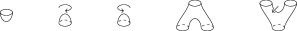
Figure 2.1. The cobordisms that generate $\mathcal{C}hron\mathcal{C}ob^{3}_{gen}$

We then mod out by orientation reversal relations, associativity and Frobenius relations, commutativity relations, cross and diamond relations, pruning relations, sphere (S) and torus (T) relations, and the four tube (4Tu) relation to arrive at $\mathcal{C}hron\mathcal{C}ob^{3}_{gen}$.

Remark 1.

When we refer to relations being associative and commutative, we mean in terms of the odd Frobenius algebra. When looking at actual cobordisms, almost all of the relations are commutativity relations in a sense, as they relate to some commutation in time of saddles or other elementary cobordisms.

Remark 2.

The cobordisms in this paper are always embedded. In [Put13] the author works with non-embedded cobordisms except for a brief period where it is strictly necessary that he work with embedded cobordisms. Working with non-embedded cobordisms simplifies the presentation of relations, in that one does not need to concern themselves with all the ways circles could be embedded in relation to one another. For the following section the non-embedded versions of relations are presented but should be interpreted as providing the relation to all of the ways circles could be embedded around one another.

Remark 3.

With regard to chronological changes, our basic cobordisms can be classified as either even or odd. Births and merges are even, while deaths and splits are odd. If a change in chronology exchanges the order of an even cobordism with any other cobordism, both cobordisms are equal. When two odd cobordisms are chronologically rearranged, multiplication by $\pi$ is incurred. With regard to orientation changes For tracking orientations splits and deaths induce multiplication by $\pi$ while merges incur no defect as a result the orientations will often be suppressed on merges.

Orientation Reversal Relations

(4)

(5)

(6)

Associativity and Frobenius Relations

(7)

(8)

(9)

Commutativity Relations

(10)

(11)

(12)

(13)

(14)

(15)

(16)

(17)

(18)

(19)

Cross and Diamond Relations

(20)

(21)

(22)

“Pruning” Relations

(23)

Sphere and Torus Relations

(24)

(25)

Four Tube Relation

(26)

Definition 4.

We say elements are $\pi$-commuting if exchanging their order induces multiplication by $\pi$. Furthermore we write $A\stackrel{{\scriptstyle\pi}}{{=}}B$—similarly for “$\simeq$”—to mean $A=B$ or $A=\pi B$.

2.3   Emergent Relations

One particular consequence of the relations described above is the handle (H) relation.

(27)

The following consequences of the (4Tu) relation will be used later

(28)

(29)

(30)

2.4   The Target Category: $\textnormal{Kom}^{b}(\textnormal{Mat}(\mathcal{C}hron\mathcal{C}ob^{3}_{gen}))$

Our final goal is to assign a homological algebra type object to each link cobordism. Objects in the category $\mathcal{C}hron\mathcal{C}ob^{3}_{gen}$ are those we will want to take chain complexes of, but before we do so we must guarantee that the category we are working with is additive. To this end, we replace $\mathcal{C}hron\mathcal{C}ob^{3}_{gen}$ with $\textnormal{Mat}(\mathcal{C}hron\mathcal{C}ob^{3}_{gen})$, where $\textnormal{Mat}(\mathcal{A})$ denotes the additive closure of the preadditive category $\mathcal{A}$. Its objects are finite (possibly empty) sequences of objects in $\mathcal{A}$, and its morphisms are given by matrices of morphisms in $\mathcal{A}$. The composition is modeled on ordinary matrix multiplication.

We can now consider the category $\textnormal{Kom}(\textnormal{Mat}(\mathcal{C}hron\mathcal{C}ob^{3}_{gen}))$ of bounded chain complexes and chain maps in $\textnormal{Mat}(\mathcal{C}hron\mathcal{C}ob^{3}_{gen})$. Let $\textnormal{Kom}^{b}(\textnormal{Mat}(\mathcal{C}hron\mathcal{C}ob^{3}_{gen}))$ denote the corresponding homotopy category in which homotopic chain maps are identified. If we further identified chain maps with their negatives and multiples by $\pi$—notated as $\textnormal{Kom}^{b}_{\pm,\pi}(\textnormal{Mat}(\mathcal{C}hron\mathcal{C}ob^{3}_{gen}))$—the generalized Khovanov bracket would be a functor from $\mathcal{C}ob^{4}$ to this category. It is simpler to work with $\textnormal{Kom}^{b}(\textnormal{Mat}(\mathcal{C}hron\mathcal{C}ob^{3}_{gen}))$ in which the generalized Khovanov bracket is only functorial up to multiplication by signs.

Remark 4.

The category where the odd Khovanov bracket resides is $\textnormal{Kom}^{b}(\textnormal{Mat}(\mathcal{C}hron\mathcal{C}ob^{3}_{odd}))$ which can be constructed either by setting $\pi=-1$ in $\textnormal{Kom}^{b}(\textnormal{Mat}(\mathcal{C}hron\mathcal{C}ob^{3}_{gen}))$ or by going through the same construction as for $\textnormal{Kom}^{b}(\textnormal{Mat}(\mathcal{C}hron\mathcal{C}ob^{3}_{gen}))$ but setting $\pi=-1$ in all of the relations. Similarly for the even Khovanov bracket except we set $\pi=1$ and arrive at $\textnormal{Kom}^{b}(\textnormal{Mat}(\mathcal{C}ob^{3}_{even}))$, by setting $\pi=1$ we essentially erase all chronological structure.

The odd Khovanov bracket is functorial up to sign in $\textnormal{Kom}^{b}(\textnormal{Mat}(\mathcal{C}hron\mathcal{C}ob^{3}_{odd}))$ and is actually a functor from $\mathcal{C}ob^{4}$ to $\textnormal{Kom}^{b}_{\pm}(\textnormal{Mat}(\mathcal{C}hron\mathcal{C}ob^{3}_{odd}))$, the category where chain maps are identified with their negatives.

2.5   Type X and Type Y Configurations

From the convention in 3, there emerges a pair of exceptional arrangements which, a priori, are neither commuting, anticommuting, nor $\pi$-commuting as they are annihilated by 2.

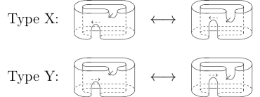
Figure 2.2. Cobordisms of type X and type Y configurations

In order to define an generalized Khovanov theory, one must artificially decide that one of these configurations commutes and that the other $\pi$-commutes. These two different generalized Khovanov theories are called type X or type Y based on which pair of cobordisms in Figure 2.2 $\pi$-commutes. It was first observed in [ORS13] that either choice produces the same final invariant, although their proof was incorrect. Putyra attempted in [Put13] to provide a corrected proof, but his proof also appears to be incorrect. This is Lemma 12, which we will prove in Section 3. We will use type Y sign assignments following Putyra in [Put13].

3   Generalized Khovanov Theory

Oriented links allow us to easily assign a direction to crossings (although it can still be defined for unoriented links using a variation on the right-hand rule). This convention is shown in Figure 3.1

Figure 3.1. Positive and negative crossings for directed links

We will now construct Putyra’s version of odd Khovanov homology. Then we will review portions of the proof of invariance, as they will be needed to extend odd Khovanov homology to link cobordisms and to prove that it is functorial. We will end this section by defining the chain maps that are assigned to each of the elementary cobordisms in $\mathcal{C}ob^{4}$.

3.1   Links with Oriented Crossings

Odd Khovanov homology is not computed from a simple link diagram, but from a link diagram that has been enhanced with orientations on the crossings. Each crossing has two possible orientations, which are displayed in Figure 3.2.

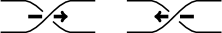
Figure 3.2. The two possible orientations on a crossing

Note that the arrows specifying the crossing orientation are chosen so that they connect the regions that lie to the left if one approaches the crossing along the overstrand from either side.

3.2   Crossing Resolution

A link diagram with $n$ crossings gives rise to $2^{n}$ planar diagrams corresponding to all possible combinations of replacing each crossing with the vertical or horizontal resolution, where the terms “vertical” and “horizontal” refer to the pictures in Figure 3.2. The rule for resolving a crossing is shown in Figure 3.3. If the crossings are labeled from 1 to $n$, then each diagram, $D_{\alpha}$, can be assigned a binary label $\alpha\in\{0,1\}^{n}$ with a 0 in the $i$^th place if the $i$^th crossing was replaced with the vertical resolution, and a 1 if it was replaced with the horizontal resolution.

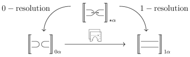
Figure 3.3. The vertical and horizontal resolution of a crossing

Convention 3.

To denote that an index is in superposition we use a $\star$ at that index.

We assign a cobordism $d_{{\dots}\star{\dots}}:D_{{\dots}0{\dots}}\rightarrow D_{{\dots}1{\dots}}$ to each pair of planar diagrams that differ by a single resolution. The cobordism $d_{{\dots}\star{\dots}}$ is a morphism in $\mathcal{C}ob^{3}$ whose initial frame is the vertical resolution and whose terminal frame is the horizontal resolution with a saddle between (as depicted in Figure 3.3). The saddle inherits its orientation from the resolved crossing’s orientation.

Convention 4.

Greek characters will be used to denote binary strings and the concatenation of Greek characters should be read as the concatenation of the binary strings. Furthermore, $\zeta$ will be used to denote the string consisting of only zeros.

Definition 5.

The degree of a resolution is the number of horizontal resolutions in the resulting diagram.

The degree of a resolution is thus the number of ones in the diagram’s binary label, and it is denoted $\deg(\alpha)$.

3.2.1   The Generalized Khovanov Bracket

Definition 6.

The cube of resolutions of a link diagram $D$ with $n$ crossings is an $n$ dimensional cube with the $2^{n}$ planar diagrams $D_{\alpha}$ for $\alpha\in\{0,1\}^{n}$ as its vertices and the corresponding cobordisms as its edges.

Each 2-dimensional face of the cube of resolutions corresponds to two vertices living in the superposition of their resolution, while all others are resolved. In order to define generalized Khovanov homology we need a chain complex. Therefore, all faces must anticommute so that the differential squares to zero. Each face falls into one of a few basic types and has an inherited sign $\sigma_{i,j}$ of either 1 or $\pi$ corresponding with the indices of the non-resolved crossings in $D_{\dots\star\dots\star\dots}$. The inherited signs appear following diagrams considered up to planar isotopy. Each tangle diagram can be closed with any crossingless tangle that connects oppositely decorated endpoints.

Figure 3.4. Commutivity of faces for type $Y$ sign assignments

  Commuting Faces (Group C) — $\sigma_{i,j}=1$

.

or

.   $\pi$-commuting Faces (Group $\pi$) — $\sigma_{i,j}=\pi$

.

or   X Face (Group X) — $\sigma_{i,j}=1$

or   Y Face (Group Y) — $\sigma_{i,j}=\pi$

or  

We need to make an assignment of a sign $\epsilon_{\dots\star\dots}$ to each edge such that

(31) $$\prod_{\{\iota_{i},\iota_{j}\}\in\{\{0,{\star}\},\{1,{\star}\},\{{\star},0\},\{{\star},1\}\}}\epsilon_{\dots\iota_{i}\dots\iota_{j}\dots}=-\sigma_{i,j}$$

Such a sign assignment can always be made ([ORS13],[Put13]), but it is not unique.

Definition 7.

The generalized Khovanov cube is the cube of resolutions with each edge multiplied by its assigned sign.

Definition 8.

The generalized Khovanov bracket is the grading-shifted flattening of the generalized Khovanov cube created by taking the direct sum of all vertices with the same degree.

The generalized Khovanov bracket is a chain complex, as all maps in the Khovanov cube raise the degree by one, and before collapsing the cube we ensured that all faces anticommute. The grading shift in the generalized Khovanov bracket is determined by the number of negative crossings in the link diagram. Note that we interpret the generalized Khovanov bracket as an object of the category $\textnormal{Kom}(\textnormal{Mat}(\mathcal{C}hron\mathcal{C}ob^{3}_{gen}))$.

Convention 5.

The unsigned cobordisms in the generalized Khovanov cube will be denoted with $d$ while the maps in the generalized Khovanov bracket are denoted with $\partial$.

Convention 6.

For a link diagram $L$ the generalized Khovanov bracket is denoted $\llbracket L\rrbracket$, additionally, the specific $\alpha$^th vertex is denoted by $\llbracket L\rrbracket_{\alpha}$ so that $\llbracket L\rrbracket_{\alpha}=D_{\alpha}$.

3.3   Odd and Generalized Khovanov TQFTs

We can construct odd or even Khovanov homology by starting with the generalized Khovanov bracket, setting $\pi$ to $-1$ or $1$, and applying the appropriate chronological TQFT functor [Put13]. Explicitly, the odd chronological TQFT functor can be defined as in [ORS13] and sends a resolution $R$ to the exterior algebra

$$F(R):=\Lambda^{*}V(R)$$

where $V(R)$ denotes the free $\mathbb{Z}$-module formally generated by the connected components of $R$. The map assigned to a planar saddle cobordism that merges two components $R_{1}$ and $R_{2}$ of $R$ is defined via the obvious quotient map $F(R)\rightarrow F(R)/(R_{1}=R_{2})$, whereas the map assigned to a split saddle is defined via the map $F(R)/(R_{1}=R_{2})\rightarrow F(R)$ induced by left-multiplication by $R_{1}-R_{2}$ (see [ORS13] for details). There is a generalized Khovanov TQFT functor that is usually defined in the language of [BN02], but that can be defined in analogy $F(R)$ by replacing the exterior algebra by the noncommutative polynomial ring over $\Bbbk$ in the components of $R$, modulo the relations

$$R_{1}R_{1}=0,\qquad R_{1}R_{2}=\pi R_{2}R_{1}$$

where $R_{1}$ and $R_{2}$ are components of $R$. These relations also imply

$$(R_{1}+\pi R_{2})R_{1}=\pi R_{2}R_{1}=R_{1}R_{2}=(R_{1}+\pi R_{2})R_{2},$$

and so the above map $F(R)/(R_{1}=R_{2})\rightarrow F(R)$ induced by left-multiplication by $R_{1}-R_{2}$ extends to the generalized setting if one instead multiplies by $R_{1}+\pi R_{2}$. In fact, the resulting map for a planar split saddle cobordism corresponds precisely to the generalized split map from [Put13].

3.4   Well Definedness of the Generalized Khovanov Bracket

To construct the generalized Khovanov bracket one must fix a diagram, fix an orientation on the crossings, and finally fix a sign assignment. To show that the generalized Khovanov bracket is well defined it is sufficient to show that these choices do not affect the homotopy type of the generalized Khovanov bracket.

3.5   Dependence on Sign Assignments and Crossing Orientations

The following lemma was shown in [ORS13, Put13]:

Lemma 1.

All valid sign assignments for a particular link diagram and fixed crossing orientations produce isomorphic generalized Khovanov brackets.

For later reference, we briefly recall the proof of this lemma.

Proof of Lemma 1..

Fix a link diagram $L$ with $n$ crossings, and let $Q$ denote the cube $[0,1]^{n}$, equipped with its usual CW structure. Further, let $o$ be a choice of crossing orientations for $L$. If we regard a sign assignment for $(L,o)$ as a cellular $1$-cochain $\epsilon\in C^{1}(Q;\Bbbk^{\times})$, then condition (31) can be written as

(32) $$\delta\epsilon=-\sigma_{L,o},$$

where $\sigma_{L,o}$ denotes the cellular 2-cochain on $Q$ defined by the $\sigma_{i,j}$. To prove the lemma, we now note that any two solutions $\epsilon$ and $\epsilon^{\prime}$ of (32) must differ by a cocycle and hence, since $Q$ is contractible, by a coboundary $\delta\eta$ of a cellular $0$-cochain $\eta\in C^{0}(Q;\Bbbk^{\times})$. The desired chain isomorphism between the generalized Khovanov brackets of $(L,o,\epsilon)$ and $(L,o,\epsilon^{\prime})$ is now given by the cubical chain map with components $\eta(\alpha)\operatorname{id}_{L_{\alpha}}\colon\llbracket L\rrbracket_{\alpha}\rightarrow\llbracket L\rrbracket_{\alpha}$ (where the term cubical means that the chain map has no nonzero components between different resolutions). ∎

In [ORS13, Put13], it was further shown that changing the orientation of a crossing does not change the generalized Khovanov bracket as long as one adjusts the sign assignment accordingly. Lemma 1 thus implies:

Lemma 2.

All choices of crossing orientations for a particular link diagram produce isomorphic generalized Khovanov brackets.

In summary, any two pairs $(o,\epsilon)$ and $(o^{\prime},\epsilon^{\prime})$ consisting of a choice crossing orientations and a valid sign assignment for a link diagram $L$ give rise to a cubical chain isomorphism

(33) $$f_{o,\epsilon}^{o^{\prime},\epsilon^{\prime}}\colon\llbracket L,o,\epsilon\rrbracket\rightarrow\llbracket L,o^{\prime},\epsilon^{\prime}\rrbracket,$$

where we are writing $\llbracket L,o,\epsilon\rrbracket$ for the generalized Khovanov bracket of $(L,o,\epsilon)$. By construction or by Lemma 3 below, this chain isomorphism is canonical up to an overall invertible scalar, and it satisfies the coherence conditions

(34) $$f_{o,\epsilon}^{o,\epsilon}=\operatorname{id}\qquad\mbox{and}\qquad f_{o^{\prime},\epsilon^{\prime}}^{o^{\prime\prime},\epsilon^{\prime\prime}}\circ f_{o,\epsilon}^{o^{\prime},\epsilon^{\prime}}=f_{o,\epsilon}^{o^{\prime\prime},\epsilon^{\prime\prime}}$$

up to an overall invertible scalar.

Lemma 3.

Let $f,g\colon\llbracket L,o,\epsilon\rrbracket\rightarrow\llbracket L,o^{\prime},\epsilon^{\prime}\rrbracket$ be cubical chain isomorphisms with components $f_{\alpha}=r_{\alpha}\operatorname{id}_{L_{\alpha}}$ and $g_{\alpha}=s_{\alpha}\operatorname{id}_{L_{\alpha}}$ for invertible scalars $r_{\alpha},s_{\alpha}\in\Bbbk^{\times}$. Then $f=cg$ for an invertible scalar $c\in\Bbbk^{\times}$.

Proof.

It suffices to show that if $f$ is a cubical chain isomorphism of the stated form, then the scalar $r_{\alpha}$ appearing at a fixed vertex $\alpha$ determines the scalars $r_{\beta}$ at all other vertices $\beta$, in the sense that $r_{\beta}/r_{\alpha}=c_{\alpha\beta}$ for a constant $c_{\alpha\beta}\in\Bbbk^{\times}$ which does not depend on $f$. Indeed, this will imply $r_{\beta}/s_{\beta}=(c_{\alpha\beta}r_{\alpha})/(c_{\alpha\beta}s_{\alpha})=r_{\alpha}/s_{\alpha}=:c$ for all $\beta$ and thus $f=cg$.

Since any two vertices in the resolution cube of $L$ can be connected by a path of edges, it further suffices to consider the case where the vertices $\alpha$ and $\beta$ are connected by an edge $e\colon\alpha\rightarrow\beta$. In this case, we have the following commuting square, in which the horizontal arrows are the differentials in $\llbracket L,o,\epsilon\rrbracket$ and $\llbracket L,o^{\prime},\epsilon^{\prime}\rrbracket$ and the vertical arrows are the relevant components of $f$:

By the remarks prior to Lemma 2, we can assume without loss of generality that $o=o^{\prime}$ and hence $d_{e}=d^{\prime}_{e}$. The commutativity of the square then implies $(r_{\beta}\epsilon_{e}-\epsilon^{\prime}_{e}r_{\alpha})d_{e}=0$ and hence, since the saddle $d_{e}$ has trivial annihilator, $r_{\beta}\epsilon_{e}=\epsilon^{\prime}_{e}r_{\alpha}$ or $r_{\beta}/r_{\alpha}=\epsilon^{\prime}_{e}/\epsilon_{e}=:c_{\alpha\beta}$. ∎

If $L$, $o$, and $Q=[0,1]^{n}$ are as in the proof of Lemma 1, then the notion of a valid sign assignment can be defined for any CW subcomplex $Q^{\prime}\subseteq Q$. Specifically, a valid sign assignment on such a subcomplex $Q^{\prime}$ is given by a cellular 1-cochain $\epsilon^{\prime}\in C^{1}(Q^{\prime};\Bbbk^{\times})$ such that $\epsilon^{\prime}=-\sigma_{L,o}|_{Q^{\prime}}$. For later use, we will prove the following lemma.

Lemma 4.

Let $Q^{\prime}\subseteq Q$ be a CW subcomplex with trivial first homology. Then any valid sign assignment on $Q^{\prime}$ extends to a valid sign assignment on $Q$.

Proof.

Let $\epsilon^{\prime}$ be a valid sign assignment on $Q^{\prime}$, and choose any valid sign assignment $\epsilon$ on $Q$. Then $\epsilon^{\prime}$ and $\epsilon|_{Q^{\prime}}$ differ by a cocycle on $Q^{\prime}$, and the assumption on $Q^{\prime}$ implies that this cocycle is a coboundary, $\delta\eta^{\prime}$, for a cellular $0$-cochain $\eta^{\prime}\in C^{0}(Q^{\prime};\Bbbk^{\times})$. To obtain a valid sign assignment on $Q$ that extends $\epsilon^{\prime}$, we now modify $\epsilon$ by $\delta\eta$, where $\eta\in C^{0}(Q;\Bbbk^{\times})$ is any extension of $\eta^{\prime}$ to $Q$. ∎

In the above proof, we can choose the 0-cochain $\eta$ to be trivial on all vertices of $Q\setminus Q^{\prime}$, in which case the modified $\epsilon$ agrees with the unmodified $\epsilon$ on all 1-cells of $Q$ whose closures are disjoint from $Q^{\prime}$. If we are given any valid sign assignment $\epsilon$ on $Q$, we can thus assume that the extended sign assignment from Lemma 4 agrees with $\epsilon$ on all such 1-cells.

3.6   Generalized Khovanov homology as a diagram and as a colimit

For a fixed link diagram $L$, let $M(L)$ denote the set of all pairs $(o,\epsilon)$ where $o$ is a choice of crossing orientations for $L$ and $\epsilon$ is a valid sign assignment for $(L,o)$:

$$M(L):=\left\{(o,\epsilon)\,\middle|\,\parbox{184.28871pt}{\centering$o$ a choice of crossing orientations for $L$ and $\delta\epsilon=-\sigma_{L,o}$\@add@centering}\,\right\}.$$

We can repackage the generalized Khovanov brackets $\llbracket L,o,\epsilon\rrbracket$ for the various possible choices of $(o,\epsilon)\in M(L)$ into a single link invariant $\llbracket L\rrbracket_{M}$, which is itself functorial. To define this invariant, let $M(L)^{\prime}$ denote the grouped whose objects are the elements of $M(L)$ and which has a single morphism between any two objects. Further, let $M(L)^{\prime\prime}$ be the set of all functors from the groupoid $M(L)^{\prime}$ to $\textnormal{Kom}^{b}_{\pm,\pi}(\mathcal{C}hron\mathcal{C}ob^{3}_{gen})$. We then define

$$\llbracket L\rrbracket_{M}\in M(L)^{\prime\prime}$$

as the functor which sends an object $(o,\epsilon)\in M(L)^{\prime}$ to the generalized Khovanov bracket of $(L,o,\epsilon)$ and the unique morphism $(o,\epsilon)\rightarrow(o^{\prime},\epsilon^{\prime})$ to the isomorphism from (33). Note that this indeed yields a functor because of the conditions in (34). Equivalently, we can view this functor as a diagram of shape $M(L)^{\prime}$ in the category $\textnormal{Kom}^{b}_{\pm,\pi}(\mathcal{C}hron\mathcal{C}ob^{3}_{gen})$.

As we shall see, the chain maps assigned to elementary link cobordisms intertwine with the isomorphisms from (33). We can rephrase this property by introducing a category $M^{\prime\prime}$ of functors valued in $\textnormal{Kom}^{b}_{\pm,\pi}(\mathcal{C}hron\mathcal{C}ob^{3}_{gen})$, where the morphisms between two such functors with source categories $I$ and $J$ is given by the natural transformations between the lifts of these functors to the product category $I\times J$. A smooth link cobordism between two links with diagrams $L_{0},L_{1}\subset\mathbb{R}^{2}$ then induces a morphism $\llbracket L_{0}\rrbracket_{M}\rightarrow\llbracket L_{1}\rrbracket_{M}$ in this category.

By adapting an idea from [BHL19], we can further extend the construction of $\llbracket L\rrbracket_{M}$ to arbitrary links in $\mathbb{R}^{3}$, including those that are not in general position with respect to the projection onto the $xy$-plane. For this, consider an arbitrary link $L\subset\mathbb{R}^{3}$, and let $N(L)$ denote the set of all triples $(\phi,o,\epsilon)$ such that $\phi$ is an ambient isotopy of $\mathbb{R}^{3}$ taking the link $L=\phi_{0}(L)$ to a link $\phi_{1}(L)$ in general position; and $(o,\epsilon)$ is an element of $M(D)$ where $D$ is the link diagram of $\phi_{1}(L)$.

Given two triples $(\phi,o,\epsilon),(\phi^{\prime},o^{\prime},\epsilon^{\prime})\in N(L)$, we can perform the isotopies $\phi_{1-t}$ and $\phi^{\prime}_{t}$ one after the other to obtain an isotopy from $\phi_{1}(L)$ to $\phi^{\prime}_{1}(L)$. The latter isotopy corresponds to a link cobordism, which induces a chain isomorphism

(35) $$f_{\phi,o,\epsilon}^{\phi^{\prime},o^{\prime},\epsilon^{\prime}}\colon\llbracket D,o,\epsilon\rrbracket\longrightarrow\llbracket D^{\prime},o^{\prime},\epsilon^{\prime}\rrbracket$$

where $D$ and $D^{\prime}$ denote planar diagrams of the links $\phi_{1}(L)$ and $\phi^{\prime}_{1}(L)$, respectively. As we did for $M(L)$, we can now replace $N(L)$ by the corresponding groupoid $N(L)^{\prime}$. The generalized Khovanov brackets of the $(D,o,\epsilon)$ together with the isomorphisms from (35) then determine a diagram of shape $N(L)^{\prime}$ or, equivalently, an element

$$\llbracket L\rrbracket_{N}\in N(L)^{\prime\prime}$$

in the set $N(L)^{\prime\prime}$ of functors from $N(L)^{\prime}$ to to $\textnormal{Kom}^{b}_{\pm,\pi}(\mathcal{C}hron\mathcal{C}ob^{3}_{gen})$. By the results of this paper, $\llbracket L\rrbracket_{N}$ is functorial in the sense that any smooth link cobordism between two links $L_{0},L_{1}\subset\mathbb{R}^{3}$ induces a morphism $\llbracket L_{0}\rrbracket_{N}\rightarrow\llbracket L_{1}\rrbracket_{N}$ in the category $M^{\prime\prime}$ defined above.

We can obtain a more concrete link invariant by fixing a bidegree $(i,j)\in\mathbb{Z}^{2}$ and replacing each generalized Khovanov bracket $\llbracket D,o,\epsilon\rrbracket$ that appears in the above construction by the corresponding generalized Khovanov homology group in bidegree $(i,j)$. After modding out by the multiplicative action of $\Bbbk^{\times}$, these generalized Khovanov homology groups become sets $S(D,o,\epsilon,i,j)$, and thus the invariant $\llbracket L\rrbracket_{N}$ becomes a diagram in the category of sets. Taking the colimit of this diagram now yields a set

$$S(L,i,j):=\left.\left(\quad\,\,\,\,\bigsqcup_{\mathclap{(\phi,o,\epsilon)\in N(L)}}S(D,o,\epsilon,i,j)\right)\middle/\left(x\sim g_{\phi,o,\epsilon}^{\phi^{\prime},o^{\prime},\epsilon^{\prime}}(x)\right)\right.$$

where $g_{\phi,o,\epsilon}^{\phi^{\prime},o^{\prime},\epsilon^{\prime}}$ denotes the map $S(D,o,\epsilon,i,j)\rightarrow S(D^{\prime},o^{\prime},\epsilon^{\prime},i,j)$ that corresponds to the isomorphism from (35). The set $S(L,i,j)$ can be defined for arbitrary links in $\mathbb{R}^{3}$, but not for arbitrary links in $S^{3}$. By the results of this paper, it is functorial in the sense that any smooth link cobordism $F\colon L\rightarrow L^{\prime}$ in $\mathbb{R}^{3}\times[0,1]$ induces a map $S(L,i,j)\rightarrow S(L^{\prime},i,j+\chi(F))$.

Note that in the remainder of this paper, we will almost always ignore the constructions of this subsection and instead work with the generalized Khovanov bracket $\llbracket L\rrbracket:=\llbracket L,o,\epsilon\rrbracket$ for a fixed link diagram $L\subset\mathbb{R}^{2}$ and a fixed choice of $(o,\epsilon)\in M(L)$.

3.7   Invariance under Reidemeister moves

Since we will need the relevant chain maps later, we will briefly summarize the proof that the generalized Khovanov bracket is invariant under Reidemeister moves, up to homotopy equivalence.

Note that in the pictures in this subsection, all critical points are assumed to be oriented as in Convention 2, so that deaths are oriented clockwise, and saddles are oriented to the right or to the front. In diagrams (36) and (37) below, we further assume that the terms sitting vertically above each other are equipped with the same internal sign assignments, and in diagram (39), we make the same assumption about the terms that are connected by an identity map.

Lemmas 5 through 7 below were shown by Putyra [Put13].

Lemma 5 (Reidemeister I invariance).

The chain maps depicted in (36) and (37) form strong deformation retractions from the top complexes to the bottom complexes.

(36)

(37)

If in the above diagrams the orientation of the crossing is flipped, then the orientations of the saddles in the differentials will be flipped as well, but the orientations of the saddles in the chain maps would still the be the ones dictated by Convention 2.

In diagram (36), $S(L_{0},\alpha)$ is the integer

(38) $$S(L_{0},\alpha):=\frac{c(L_{0},\alpha)+c(L_{0},\zeta)+deg(\alpha)}{2}$$

where $L_{0}$ denotes the link diagram in the bottom row, and $c(L_{0},\alpha)$ and $c(L_{0},\zeta)$ denote respectively the numbers of circles in the resolution $\alpha$ and in the all-zero resolution $\zeta$.

The function $S(L_{0},-)$ appeared in similar form in [Man14]. It is defined such that across a merge differential in the resolution cube of $L_{0}$, the increase in the degree and the decrease in the number of components cancel out, while across a split differential, they add up to increment $S(L_{0},\alpha)$ by $1$. The term $c(L_{0},\zeta)$ is to ensure that $S(L_{0},\alpha)$ is an integer. Note that the choice of this term is somewhat arbitrary. We could instead replace it by its negative, or replace $\zeta$ by any fixed resolution of $L_{0}$, such as the oriented resolution. This would at most change the chain maps in (36) by an overall factor of $\pi$.

Lemma 6 (Reidemeister II invariance).

The chain maps depicted in (39) form a strong deformation retraction from the bottom complex to the top complex.

(39)

In the above definition of $f$, the constant $a$ takes on the value 1 if the right crossing is oriented downward—as shown in the diagram—and the value $\pi$ if it is oriented upward. The saddles in $f$ and $g$ inherit their orientations from the directions of the arrows at the left and right crossing, respectively, and the death in $f$ is always oriented clockwise.

To prove invariance under Reidemeister III moves, Putyra uses that the generalized Khovanov brackets on the two sides of the move can be viewed as mapping cones, as shown below.

(40)

(41)

The homotopy type of a mapping cone of a chain map does not change if one composes the chain map with a homotopy equivalence. Lemma 6 thus implies that the above mapping cones are homotopy equivalent to the ones below (where the rightmost maps in (42) and (43) are induced by inverse Reidemeister II moves):

(42)

(43)

Now let $\Phi_{L}$ and $\Phi_{R}$ denote the composed chain maps that appear in the cones on the right-hand sides of (42) and (43), respectively. After choosing sign assignments appropriately, we can assume that $\Phi_{L}$ and $\Phi_{R}$ have the same source complex and the same target complex. Invariance under Reidemeister III moves then follows from the lemma below.

Lemma 7 (Reidemeister III invariance).

$\Phi_{L}$ and $\Phi_{R}$ are identical, up to a possible overall invertible scalar.

Since Putyra’s proof of this lemma omitted some of the details, we here give a more thorough argument, based on the proof of a corresponding result from [ORS13].

Proof of Lemma 7.

The diagrams in (44) and (45) below depict the maps $\Phi_{L}$ and $\Phi_{R}$ more explicitly. For the present argument, we need to consider the maps which travel up these diagrams. There is a second version of the Reidemeister III move where the crossing that travels over the lowest strand is reversed, so that the roles of its $0$- and $1$-resolution are exchanged. For that version of the move, one would need to consider the maps traveling down the diagrams, but the argument would otherwise be essentially identical.

(44)

(45)

A careful investigation of the chain maps in (39), (44), and (45) now reveals that the nonzero components of $\Phi_{L}$ and $\Phi_{R}$ (and of the maps in reverse direction) are given by the following underlying cobordisms:

(46)

(47)

This shows that the maps $\Phi_{L}$ and $\Phi_{R}$ are the same when coefficients in $\Bbbk^{\times}$ are stripped away. What remains is to show that the coefficients in the cone in (42) are consistent with those in the cone in (43). To see this, note that the cone on the right-hand side of (42) contains two obvious quotient complexes, which are both cubical. The first of these is given by the bottom layer of (44), whereas the second one is obtained from the entire mapping cone by removing the term that sits at the rightmost vertex in the bottom layer of (44).

Corresponding to these two quotient complexes, we consider two $(n-1)$-dimensional cubes $Q\cong[0,1]^{n-1}$ and $Q^{\prime}\cong[0,1]^{n-1}$, where $n$ denotes the number of crossings in the link diagrams that show up on either side of the Reidemeister III move. Let $P\coloneqq Q\cup Q^{\prime}$ be the CW complex obtained by gluing the cubes $Q$ and $Q^{\prime}$ along the two $(n-2)$-dimensional subcubes that correspond to the two edges on the left side of the bottom layer of (44).

It is easy to see that the signs coming from (42) define a valid sign assignment on $P$, in an obvious sense. We can think of this sign assignment as a cellular 1-cochain $\epsilon\in C^{1}(P;\Bbbk^{\times})$, and there is a similar cellular 1-cochain $\epsilon^{\prime}\in C^{1}(P;\Bbbk^{\times})$ coming from the signs in (43). Because of our choices, it follows that $\epsilon$ and $\epsilon^{\prime}$ must differ by a relative cocycle in $Z^{1}(P,Q\cup T;\Bbbk^{\times})$, where $T\cong[0,1]^{n-2}$ corresponds to the top-most term in (44). The lemma now follows because $Z^{1}(P,Q\cup T;\Bbbk^{\times})\cong H^{1}(P/(Q\cup T);\Bbbk^{\times})\cong H^{1}(S^{1};\Bbbk^{\times})\cong\Bbbk^{\times}$. ∎

While in principle, there could be many different homotopy equivalences between the complexes on the two sides of a Reidemeister move, the specific homotopy equivalences considered in this subsection are unique (or unique up to overall invertible scalars). In each of the moves, we placed some restrictions on the relationship between the chosen sign assignments before and after the move. These restrictions can easily be lifted by composing the chain maps discussed in this subsection with the isomorphisms from (33). The resulting chain maps are still unique up to invertible scalars and natural with respect to the choice of $(o,\epsilon)$, and thus induce well-defined morphisms $\llbracket L_{0}\rrbracket_{M}\rightarrow\llbracket L_{1}\rrbracket_{M}$ in the category $M^{\prime\prime}$ from the previous subsection.

3.8   Equivalence of type X and type Y assignments

We still need to prove Theorem 2 about the equivalence of type X and type Y theories.

In the following, let $D\subset\mathbb{R}^{2}$ be a link diagram in the $xy$-plane representing a link $L\subset\mathbb{R}^{3}$. Moreover, let $D^{\prime}$ be the diagram of the rotated link $L^{\prime}:=\rho_{1}(L)$, where $\rho_{t}\colon\mathbb{R}^{3}\rightarrow\mathbb{R}^{3}$ is the rotation by $180t$ degrees about the $y$-axis $\lambda\subset\mathbb{R}^{3}$. Note that, on the level of diagrams in the $xy$-plane, $D^{\prime}$ can be obtained from $D$ by first reflecting $D$ along $\lambda$, and then reversing the over/undercrossing information at each crossing of the resulting reflected diagram.

Let $o$ be a choice of crossing orientations for $D$, and $o^{\prime}$ be the corresponding reflected choice for $D^{\prime}$. Moreover, let $\epsilon$ and $\epsilon^{\prime}$ be fixed type X sign assignments for $(D,o)$ and $(D^{\prime},o^{\prime})$, respectively. The links $\rho_{t}(L)$ for $t\in[0,1]$ define an ambient isotopy from $L$ to $L^{\prime}$, and there is thus an induced homotopy equivalence

(48) $$\llbracket D,o,\epsilon\rrbracket\simeq\llbracket D^{\prime},o^{\prime},\epsilon^{\prime}\rrbracket,$$

which is defined uniquely up to homotopy and invertible scalars. Now consider any smooth link cobordism $F\colon L_{0}\rightarrow L_{1}$, and let

(49) $$F^{\prime}:=(\rho_{1}\times\operatorname{id}_{I})(F)\subset\mathbb{R}^{3}\times I$$

denote the corresponding rotated link cobordism between the rotated links $L_{0}^{\prime}$ and $L_{1}^{\prime}$. Further, let $\Phi^{Y}_{F}$ and $\Phi^{Y}_{F^{\prime}}$ denote the type X maps that $F$ and $F^{\prime}$ induce between the generalized Khovanov brackets of type Y. We then claim:

Lemma 8.

The homotopy equivalence in (48) is natural, in the sense that it intertwines the maps $\Phi^{Y}_{F}$ and $\Phi^{Y}_{F^{\prime}}$ up to homotopy and an overall invertible scalar.

Proof.

This follows directly from the functoriality of the generalized Khovanov bracket because the relevant compositions that need to be compared to establish the naturality of (48) are induced by ambient isotopic link cobordisms. ∎

Now note that the crossings of $D^{\prime}$ correspond canonically to those of $D$, and, under this correspondence, the type Y assignment $\epsilon^{\prime}$ for $(D^{\prime},o^{\prime})$ can be seen as a type X assignment for the original diagram $(D,o)$. We also have

(50) $$\mathcal{R}(\llbracket D^{\prime},o^{\prime},\epsilon^{\prime}\rrbracket)=\llbracket D,o,\epsilon^{\prime}\rrbracket,$$

where $\mathcal{R}$ denotes the endofunctor of $\textnormal{Kom}^{b}(\mathcal{C}hron\mathcal{C}ob^{3}_{gen})$ given by reflecting objects across $\lambda\subset\mathbb{R}^{2}$, and chronological cobordisms $S\subset\mathbb{R}^{2}\times I$ (including the orientations of their critical points) across $\lambda\times I\subset\mathbb{R}^{2}\times I$. Given a link cobordism $F$, let $\Phi^{X}_{F}$ denote the type X map that $F$ induces on the generalized Khovanov bracket of type X. Assuming that $F^{\prime}$ is the rotated link cobordism as in equation (49), we have:

Lemma 9.

The equality in (50) is natural, in the sense that $\mathcal{R}(\Phi^{Y}_{F^{\prime}})$ coincides with $\Phi^{X}_{F}$ up to an overall invertible scalar.

Proof.

It suffices to prove this when $F$ is an elementary link cobordism. If $F$ is a birth, then the statement is obvious. If $F$ is a death, then $\mathcal{R}(\Phi^{Y}_{F^{\prime}})$ and $\Phi^{X}_{F}$ differ by a factor of $\pi$ because $\mathcal{R}$ reverses the orientation of each planar death cobordism that appears in the chain map $\Phi^{Y}_{F^{\prime}}$.

If $F$ is a saddle cobordism, then the chain maps $\Phi^{X}_{F}$ and $\Phi^{Y}_{F^{\prime}}$ are defined via type X and type Y assignments $\widetilde{\epsilon}$ and $\widetilde{\epsilon}^{\prime}$ on the cubes of larger link diagrams $(\widetilde{D},\widetilde{o})$ and $(\widetilde{D}^{\prime},\widetilde{o}^{\prime})$, respectively. In this case, the lemma follows because $\mathcal{R}$ takes $\llbracket\widetilde{D},\widetilde{o},\widetilde{\epsilon}\rrbracket$ to $\llbracket\widetilde{D}^{\prime},\widetilde{o}^{\prime},\widetilde{\epsilon}^{\prime}\rrbracket$.

It remains to consider the case where $F$ is induced by a Reidemeister move. For a negative Reidemeister I move, the maps $\mathcal{R}(\Phi^{Y}_{F^{\prime}})$ and $\Phi^{X}_{F}$ are the same as in each map the orientation reversals on split saddles and deaths will cancel. For a positive Reidemeister I move, the maps $\mathcal{R}(\Phi^{Y}_{F^{\prime}})$ and $\Phi^{X}_{F}$ differ by $\pi$ as orientation reversals on splits and deaths appear alone. For a Reidemeister II move, the maps $\mathcal{R}(\Phi^{Y}_{F^{\prime}})$ and $\Phi^{X}_{F}$ feature the same orientations on the saddle in the non-identity maps in the map with a death, the orientation change on the death is canceled by the change in the “a” term, and overall the maps are the same.

Finally, the components of the Reidemeister III chain maps are given by identity maps, Reidemeister II chain maps, and compositions af homotopies, differentials, and Reidemeister II chain maps. we have already seen that components coming from differentials and Reidemeister II chain maps are the same in $\mathcal{R}(\Phi^{Y}_{F^{\prime}})$ and $\Phi^{X}_{F}$.

The see that the same is true for components coming from homotopies, we note that the relevant homotopies are given by the death in $f$ accompanied by the sign $-a\pi\epsilon_{0,0\star\alpha}$, and by the birth in $g$, accompanied by the sign $-\epsilon_{0,1\star\alpha}$, where we are referring to the notations from (39). The same analysis that we used for the maps $f$ and $g$ thus Shows that the components coming from these homotopies Are also the same in $\mathcal{R}(\Phi^{Y}_{F^{\prime}})$ and $\Phi^{X}_{F}$.

∎

If we could show that $\mathcal{R}$ is naturally isomorphic to the identity functor, then Theorem 2 would follow from equations (48) and (50) and from the preceding lemmas. We will instead show a weaker property of $\mathcal{R}$.

For an object $C\subset\mathbb{R}^{2}$ of the embedded category, let $S_{C}\colon C\rightarrow\mathcal{R}(C)$ denote a cobordism which connects each component of $C$ to the corresponding reflected component of $\mathcal{R}(C)$ using a genus zero cobordism with no critical points.

Lemma 10.

Any choice of map $S_{C}$ is equal to any other choice.

Proof.

The diagram $C$ in $\mathbb{R}^{3}$ consists of nested circles. We can enumerate the circles in $C$, and divide the circles into disjoint sets corresponding to which other circle they are directly nested inside. The diagram $\mathcal{R}(C)$ can inherit the enumeration from $C$ and thus for each set of circles $B_{i}$ with $k_{i}$ circles, the cobordism $S_{C}$ associates an element of $\mathcal{B}_{k_{i}}$ the braid group with $k_{i}$ generators. Overall to $C$, $S_{C}$ associates an element of the group $\displaystyle\prod_{i\in I}\mathcal{B}_{k_{i}}$. If all the circle in a set $B_{i}$ have no circles nested inside them, the four-tube relation gives us the following:

(51)

In the braid group this corresponds with the extra relation that generators square to identity. Making this additional identification we are left with $\mathcal{S}_{k_{i}}$ the symmetric group with $k_{i}$ generators. If we could do this for each $B_{i}$, $S_{C}$ would induce an element of $\displaystyle\prod_{i\in I}\mathcal{S}_{k_{i}}$ in turn indicating that all choices for $S_{C}$ are equivalent as they correspond to the identity permutation of the circles.

If we look at the relation from before there is a gray region in the core of the right cobordism. We can fill fill this region in with a cobordism indicating that the additional relation also applies to pairs of circles, as long as one them contains no other circles.

In the event that two circles in the set $B_{i}$ themselves contain circles consider the following decomposition

(52)

In essence working from the inside out, the cobordisms inside of a cobordism can be “absorbed” into the wall of the outer cobordism we can then leave the “B” portion of the decomposition below and push the “A” portion above the twisted cobordisms. After we apply the earlier relation, we can slide all of the “B” and “A” sections back together without incurring any signs as we never need to change the orientation on a saddle or change the chronology. ∎

We cannot build a chain map between $\llbracket D^{\prime},o^{\prime},\epsilon^{\prime}\rrbracket$ and $\mathcal{R}(\llbracket D^{\prime},o^{\prime},\epsilon^{\prime}\rrbracket$ by just using the map $S_{C}$ on each resolved crossing diagram $C$ as it would not commute with the differential. If we make appropriate choices of $S_{C}$ it is clear that a merge cobordism will commute with the reflection map, while a split cobordism induces a $\pi$ associated with the reflection reversing the orientation on the split. It follows that there is a cubical chain isomorphism

(53) $$\Psi\colon\llbracket D^{\prime},o^{\prime},\epsilon^{\prime}\rrbracket\longrightarrow\mathcal{R}(\llbracket D^{\prime},o^{\prime},\epsilon^{\prime}\rrbracket)$$

with components $\Psi_{\alpha}:=\pi^{S(D^{\prime},\alpha)}S_{D^{\prime}_{\alpha}}$ where the exponent $S(D^{\prime},\alpha)\in\mathbb{Z}$ is defined as in (38).

Lemma 11.

The chain isomorphism in (53) is natural, in the sense that it intertwines the maps $\Phi^{Y}_{F^{\prime}}$ and $\mathcal{R}(\Phi^{Y}_{F^{\prime}})$ up to an overall invertible scalar.

Proof.

We leave the proof of the lemma to the reader as it is simlar to the computations in Subsection 4.4. It is sufficient to verify that for $F$ an elementary link cobordism $\Phi^{Y}_{F^{\prime}}\stackrel{{\scriptstyle\pi}}{{=}}\Psi_{\alpha}^{-1}\circ\mathcal{R}(\Phi^{Y}_{F^{\prime}})\circ\Psi_{\alpha}$. It is helpful to note that the process of reflecting a death cobordism induces multiplication by $\pi$ as it reverses the orientation on the death. ∎

Combing equations (48), (50), and (53), we now obtain a homotopy equivalence

(54) $$\llbracket D,o,\epsilon\rrbracket\,\simeq\,\llbracket D^{\prime},o^{\prime},\epsilon^{\prime}\rrbracket\,\stackrel{{\scriptstyle\Psi}}{{\cong}}\,\mathcal{R}(\llbracket D^{\prime},o^{\prime},\epsilon^{\prime}\rrbracket)\,=\,\llbracket D,o,\epsilon^{\prime}\rrbracket$$

between the type Y complex $\llbracket D,o,\epsilon\rrbracket$ and the type X complex $\llbracket D,o,\epsilon^{\prime}\rrbracket$. Moreover, Lemmas 8, 9, and 11 imply that this homotopy equivalence is natural, which proves Theorem 2 As an immediate corollary, we obtain a correct proof of the following lemma, which was first stated as Lemma 2.4 in [ORS13].

Lemma 12.

Type X and type Y sign assignments yield isomorphic odd Khovanov complexes.

Proof.

By (54), the odd Khovanov complexes of $(D,o,\epsilon)$ and $(D,o,\epsilon^{\prime})$ are homotopy equivalent. The two complexes are also bounded complexes of finitely generated free abelian groups, which share the same chain ranks. An argument related to the Smith normal form of an integer matrix now shows that two such complexes are homotopy equivalent if and only if they are isomorphic. The lemma thus follows. ∎

Note that the isomorphism from the proof of Lemma 12 might not be natural.

3.9   Definition of the Generalized Khovanov Functor

In this subsection, we will define the generalized Khovanov chain maps assigned to each elementary link cobordism. Note that the definition of such maps was already sketched in [Put13].

For a link cobordism $F$ from the link diagram $L_{0}$ to the link diagram $L_{1}$, we will denote the associated chain map on the generalized Khovanov bracket by $\Phi=\Phi_{F}\colon\llbracket L_{0}\rrbracket\rightarrow\llbracket L_{1}\rrbracket$. The chain maps that we will assign to birth, death, and saddle cobordisms will preserve the cubical structure of the Khovanov bracket, meaning that their nonzero components will be between corresponding vertices in the cubes of $L_{0}$ and $L_{1}$. For such maps $\Phi$, the particular component going from $\llbracket L_{0}\rrbracket_{\alpha}$ to $\llbracket L_{1}\rrbracket_{\alpha}$ will be denoted $\Phi_{\alpha}$, while the planar cobordism underlying $\Phi_{\alpha}$ will be denoted $\varphi_{\alpha}$.

3.9.1   Birth Cobordisms

Let $F\colon L_{0}\rightarrow L_{1}$ be a four-dimensional birth cobordism, so that $L_{1}$ is the disjoint union of $L_{0}$ with a circle. For each $\alpha$ we define $\varphi_{\alpha}$ as the identity cobordism on the components of $\llbracket L_{0}\rrbracket_{\alpha}$ together with planar birth cobordism ending in the new circle in $\llbracket L_{1}\rrbracket_{\alpha}$. As births are even, the $\varphi_{\alpha}$ already commute with the differentials, and we thus obtain a chain map $\Phi\colon\llbracket L_{0}\rrbracket\rightarrow\llbracket L_{1}\rrbracket$ by setting $\Phi_{\alpha}:=\varphi_{\alpha}$.

3.9.2   Death Cobordisms

Let $F\colon L_{0}\rightarrow L_{1}$ be a four-dimensional death cobordism, so that $L_{0}$ is the disjoint union of $L_{1}$ with a circle. For each $\alpha$ we define $\varphi_{\alpha}$ as the identity cobordism on components of $\llbracket L_{0}\rrbracket_{\alpha}$ that are also present in $\llbracket L_{1}\rrbracket_{\alpha}$ and as a planar death cobordism on the lone circle in $\llbracket L_{0}\rrbracket_{\alpha}$. Unlike births, deaths can either commute or $\pi$-commute with differentials. To make them commute, we need to multiply the $\varphi_{\alpha}$ by $\pi^{S(L_{0},\alpha)}$, where $S(L_{0},\alpha)$ denotes the quantity from equation (38). Thus, the chain map $\Phi\colon\llbracket L_{0}\rrbracket\rightarrow\llbracket L_{1}\rrbracket$ assigned to an elementary death cobordism has components $\Phi_{\alpha}:=\pi^{S(L_{0},\alpha)}\varphi_{\alpha}$.

3.9.3   Saddle Cobordisms

Let $F\colon L_{0}\rightarrow L_{1}$ be a four-dimensional saddle cobordism. For each $\alpha$, the planar diagrams $\llbracket L_{0}\rrbracket_{\alpha}$ and $\llbracket L_{1}\rrbracket_{\alpha}$ are related by a saddle in the neighborhood where $L_{0}$ and $L_{1}$ differ. Consider the larger link diagram $L$ which has one extra crossing in this neighborhood, so that replacing this crossing by its 0- or 1-resolution yields the diagrams $L_{0}$ and $L_{1}$, respectively. By construction, the resolution cube of $L$ contains the resolution cubes of $L_{0}$ and $L_{1}$ as codimension-1 subcubes, and by Lemma 4, we can find a sign assignment for the resolution cube of $L$ which restricts to the given sign assignments for $L_{0}$ and $L_{1}$. Consider the components $\partial_{\alpha\star}\colon\llbracket L_{0}\rrbracket_{\alpha}\rightarrow\llbracket L_{1}\rrbracket_{\alpha}$ of the differential in $\llbracket L\rrbracket$ that pass between the two subcubes. These components are of the form

(55) $$\partial_{\alpha\star}=\epsilon_{\alpha\star}d_{\alpha\star}$$

for planar saddle cobordisms $d_{\alpha\star}\colon\llbracket L_{0}\rrbracket_{\alpha}\rightarrow\llbracket L_{1}\rrbracket_{\alpha}$, where the coefficients $\epsilon_{\alpha,\star}\in\Bbbk^{\times}$ ensure that the $\partial_{\alpha\star}$ anticommute with the differentials in $\llbracket L_{0}\rrbracket$ and $\llbracket L_{1}\rrbracket$. We can thus define a chain map $\Phi\colon\llbracket L_{0}\rrbracket\rightarrow\llbracket L_{1}\rrbracket$ by setting $\Phi_{\alpha}:=(-1)^{\deg(\alpha)}\partial_{\alpha\star}$.

We claim that the above definition specifies the saddle map $\Phi$ uniquely up to an overall invertible scalar. Indeed, let $Q\cong[0,1]^{n+1}$ denote the hypercube corresponding to $L$, and $Q_{0}$ and $Q_{1}$ denote the subcubes corresponding to $L_{0}$ and $L_{1}$. For fixed sign assignments on $Q_{0}$ and $Q_{1}$, any two choices for the $\epsilon_{\alpha\star}$ in (55) then differ by a relative 1-cocycle in $Z^{1}(Q,Q_{0}\cup Q_{1};\Bbbk^{\times})$. The claim now follows because

$$Z^{1}(Q,Q_{0}\cup Q_{1};\Bbbk^{\times})\cong H^{1}(Q/(Q_{0}\cup Q_{1});\Bbbk^{\times})\cong H^{1}(S^{1};\Bbbk^{\times})\cong\Bbbk^{\times}.$$

We further observe that changing the orientation of the extra crossing in $L$ leaves the chain complex of $L$ and hence the chain map $\Phi$ unchanged if one adjusts the sign assignment for $L$ appropriately (this follows essentially from the proof Lemma 2.3 in [ORS13]). Similarly, changing the orientation of a crossing in $L_{0}$ or $L_{1}$ leaves $\Phi$ unchanged if one changes the sign assignments for $L$ appropriately. Finally, $\Phi$ is natural in the choice of the sign assignments for $L_{0}$ and $L_{1}$, and thus it induces a morphism $\llbracket L_{0}\rrbracket_{M}\rightarrow\llbracket L_{1}\rrbracket_{M}$ in the category $M^{\prime\prime}$ from Subsection 3.6 (the latter is also trivially true for the chain maps that we assigned to birth and death cobordisms).

We briefly consider the special case in which $L_{0}$ is a union of two disjoint link diagrams and $F$ merges these diagrams into a connected sum diagram $L_{1}$. In this case, we can use the same sign assignments for $L_{0}$ and $L_{1}$ because these diagrams have the same commutativity cocylces $\sigma_{i,j}$. To construct the saddle map $\Phi$, we then do note need to pass to the larger link diagram $L$. Instead, the components of $\Phi$ are given by the same underlying saddle cobordisms $\varphi_{\alpha}\colon\llbracket L_{0}\rrbracket_{\alpha}\rightarrow\llbracket L_{1}\rrbracket_{\alpha}$ as in the general case, but now all of these saddles are merges, and the $\epsilon_{\alpha\star}$ are trivial (i.e., $\Phi_{\alpha}:=\varphi_{\alpha}=d_{\alpha\star}$). The case where $L_{0}$ is a connected sum and $F$ splits this diagram into the corresponding disjoint union of two diagrams is similar. We can again use the same sign assignments for $L_{0}$ and $L_{1}$, but now all of the cobordisms $\varphi_{\alpha}\colon\llbracket L_{0}\rrbracket_{\alpha}\rightarrow\llbracket L_{1}\rrbracket_{\alpha}$ are split saddles, and the coefficients $\epsilon_{\alpha\star}$ are given explicitly by the same terms that we used for death cobordisms (i.e., $\Phi_{\alpha}:=\pi^{S(L_{0},\alpha)}\varphi_{\alpha}=\pi^{S(L_{0},\alpha)}d_{\alpha\star}$).

3.9.4   Reidemeister Type Cobordisms

To Reidemeister I and II type cobordisms, we assign the chain maps shown in (36), (37), and (39). To Reidemeister III type cobordisms, we assign the chain map induced by the homotopy equivalences in (42) and (43). Note that this chain map has the following general form:

(56)

4   The Functoriality of Generalized Khovanov Homology up to Sign

We now have all the elements in place to prove the following theorem.

Theorem 5.

Odd Khovanov homology extends to a functor from the category $\mathcal{C}ob^{4}$ to the category $\textnormal{Kom}^{b}_{\pm,\pi}(\textnormal{Mat}(\mathcal{C}hron\mathcal{C}ob^{3}_{gen}))$.

An immediate consequence of Theorem 5 is the main result of the paper, which is realized by setting $\pi=-1$ in the generalized Khovanov Bracket.

Corollary 2.

Odd Khovanov homology extends to a functor from the category $\mathcal{C}ob^{4}$ to the category $\textnormal{Kom}^{b}_{\pm}(\textnormal{Mat}(\mathcal{C}hron\mathcal{C}ob^{3}_{odd}))$.

In Section 3 we specified what generalized Khovanov homology assigns to movies of link cobordisms. The entirety of this section is devoted to the proof of Theorem 5, where we show how our construction respects all the possible basic ambient isotopies of $\mathcal{C}ob^{4}$. We will begin with a discussion of the type I movie moves, followed by a general argument to show that each side of the type II movie moves produces homotopic chain maps. Next, we will examine type III movie moves with individual arguments in the forward direction, in the reverse direction, and for alternative variants. Finally, we will show the functoriality of odd Khovanov homology with respect to chronological movie moves. We do not need to spend additional time ensuring our functor respects equivalences of planar ambient isotopy cobordisms. Such equivalences are equalities in both $\mathcal{C}ob^{4}$ and $\mathcal{C}ob^{3}$, and are thus respected by our functor.

4.1   Type I Movie Moves

Type

I

Movie

Moves

$=\left[\addstackgap[0.25em]{\begin{tabular}[]{c}\leavevmode\hbox{$\vbox{\hbox{\resizebox{}{}{{\leavevmode\hbox{\set@color{\includegraphics[scale={0.0375}]{Figures/S04-1F001.pdf}}}}}}}$}\\ MM1\end{tabular}}\begin{tabular}[]{c}\leavevmode\hbox{$\vbox{\hbox{\resizebox{}{}{{\leavevmode\hbox{\set@color{\includegraphics[scale={0.0375}]{Figures/S04-1F002.pdf}}}}}}}$}\\ MM2\end{tabular}\begin{tabular}[]{c}\leavevmode\hbox{$\vbox{\hbox{\resizebox{}{}{{\leavevmode\hbox{\set@color{\includegraphics[scale={0.0375}]{Figures/S04-1F003.pdf}}}}}}}$}\\ MM3\end{tabular}\begin{tabular}[]{c}\leavevmode\hbox{$\vbox{\hbox{\resizebox{}{}{{\leavevmode\hbox{\set@color{\includegraphics[scale={0.0375}]{Figures/S04-1F004.pdf}}}}}}}$}\\ MM4\end{tabular}\begin{tabular}[]{c}\leavevmode\hbox{$\vbox{\hbox{\resizebox{}{}{{\leavevmode\hbox{\set@color{\includegraphics[scale={0.0375}]{Figures/S04-1F005.pdf}}}}}}}$}\\ MM5\end{tabular}\right]$

Figure 4.1. Movie moves 1 through 5

The left-hand sides of the first five movie moves are given by doing and undoing a Reidemeister move, while the right-hand sides (which are not shown in Figure 4.1) are given by trivial movies of identity cobordisms. Since the chain maps assigned to Reidemeister moves are homotopy equivalences, it is clear that the left-hand sides induce chain maps homotopic to the identity, and thus our functor respects these movie moves.

4.2   Type II Movie Moves

Type

II

Movie

Moves

$=\left[\begin{tabular}[]{c}\leavevmode\hbox{$\vbox{\hbox{\resizebox{}{}{{\leavevmode\hbox{\set@color{\includegraphics[scale={0.0375}]{Figures/S04-1F006.pdf}}}}}}}$}\\ MM6\end{tabular}\begin{tabular}[]{c}\leavevmode\hbox{$\vbox{\hbox{\resizebox{}{}{{\leavevmode\hbox{\set@color{\includegraphics[scale={0.0375}]{Figures/S04-1F007.pdf}}}}}}}$}\\ MM7\end{tabular}\begin{tabular}[]{c}\leavevmode\hbox{$\vbox{\hbox{\resizebox{}{}{{\leavevmode\hbox{\set@color{\includegraphics[scale={0.0375}]{Figures/S04-1F008.pdf}}}}}}}$}\\ MM8\end{tabular}\begin{tabular}[]{c}\leavevmode\hbox{$\vbox{\hbox{\resizebox{}{}{{\leavevmode\hbox{\set@color{\includegraphics[scale={0.0375}]{Figures/S04-1F009.pdf}}}}}}}$}\\ MM9\end{tabular}\addstackgap[0.25em]{\begin{tabular}[]{c}\leavevmode\hbox{$\vbox{\hbox{\resizebox{}{}{{\leavevmode\hbox{\set@color{\includegraphics[scale={0.0375}]{Figures/S04-1F010.pdf}}}}}}}$}\\ MM10\end{tabular}}\right]$

Figure 4.2. Movie moves 6 through 10

Any link diagram on which a movie move is carried out consists of two tangles glued together: namely the inside part $t$ where the movie move is carried out, and an outside part $T$ which is carried through the movie by identity. Type II movie moves permit a slightly stricter decomposition wherein the inside tangle is isotopic to a braid diagram.

The left-hand sides of these movie moves are shown in Figure 4.2 and are given by sequences of Reidemeister moves that start and end on identical frames, while the right-hand sides are given by trivial movies of identity cobordisms. To show invariance under these moves, we will establish a general lemma pertaining to the case where the inside tangle is a braid diagram. More generally, we will allow the inside tangle to be of the form $t=C\cup\beta\subset B\cup A$ where

• $B$ is a disk region and $A$ is an annular region surrounding it,

• $C\subset B$ is a crossingless tangle with no closed components,

• $\beta\subset A$ is an affine braid, consisting of strands that are monotonous in the radial coordinate on $A$ and that connect the points of $\partial C$ to points on the outer boundary of $A$.

We then have:

Lemma 13.

Let $F$ be a link cobordism with a link diagram $D$ as both its initial and terminal frame. Furthermore, suppose $F$ is generated by performing a sequence of Reidemeister moves on a tangle $t\subset D$ of the form $t=C\cup\beta$ where $C$ and $\beta$ are as above. Then the chain map that $F$ induces on $\llbracket D\rrbracket$ is homotopic to $\pm\textnormal{id}$ or $\pm\pi\textnormal{id}$.

Proof.

Let $t=C\cup\beta=:C\beta$ be as in the lemma, and $T$ the arbitrary tangle on the outside. The link cobordism $F$ is the identity cobordism on the tangle $T$, and on the tangle $C\beta$ it is a cobordism $f$ generated by the sequence of Reidemeister moves. Let $\Phi=\Phi_{F}$ be the map that $F$ induces on the generalized Khovanov bracket of $D$:

(57)

To prove the lemma, we must show that $\Phi\simeq c\operatorname{id}$ for a $c\in\Bbbk^{\times}$. Consider the alternative diagram $D^{\prime}$ of the same link obtained by gluing the affine braid $\beta^{-1}\beta$ onto $T$, as shown in (58). The sequence of Reidemeister moves considered previously gives rise to a cobordism $F^{\prime}$ from $D^{\prime}$ to $D^{\prime}$, and this cobordism induces a map $\Phi^{\prime}$ on the generalized Khovanov bracket of $D^{\prime}$:

(58)

We can also consider the cobordism $G$ from $D$ to $D^{\prime}$ which is the identity cobordism on $C\beta$ and a cobordism $g$ comprised of many Reidemeister II type cobordisms from $T$ to $\beta^{-1}\beta T$. Let $\Psi$ be the homotopy equivalence that $G$ induces between the generalized Khovanov brackets of $D$ and $D^{\prime}$:

(59)

The chain maps induced by $F$, $F^{\prime}$, and $G$ fit into the following diagram:

(60)

Claim 1.

The preceding diagram commutes up to homotopy and overall invertible scalars.

We will wait until the end of the proof to prove this claim. The claim implies that to prove Lemma 13, it is sufficient to show:

Claim 2.

$\Phi^{\prime}\simeq c\operatorname{id}$ for $c\in\Bbbk^{\times}$.

To prove the latter claim, we consider an alternative decomposition of $D^{\prime}$ in which the affine braid $\beta\beta^{-1}$ is glued onto the perimeter of $C$ as shown in the bottom half of (61). Let $G^{\prime}$ be the link cobordism from $D$ to $D^{\prime}$ which is given by the identity cobordism of $\beta T$ and by a cobordism $g^{\prime}$ comprised of many Reidemeister II type cobordisms from $C$ to $C\beta\beta^{-1}$.

The link cobordism $G^{\prime}$ induces an alternative homotopy equivalence $\Psi^{\prime}$ between the generalized Khovanov brackets of $D$ and $D^{\prime}$:

(61)

Now consider the following automorphism of $\llbracket D\rrbracket$ where $\left(\Psi^{\prime}\right)^{-1}$ is the homotopy inverse of $\Psi^{\prime}$:

(62) $$\Phi^{\prime\prime}\coloneqq\left(\Psi^{\prime}\right)^{-1}\circ\Phi^{\prime}\circ\Psi^{\prime}$$

By the definition of $\Phi^{\prime\prime}$, the following diagram commutes up to homotopy.

(63)

To prove the Claim 2, it is thus sufficient to show the following.

Claim 3.

$\Phi^{\prime\prime}=c\operatorname{id}$ for $c\in\Bbbk^{\times}$.

To prove the latter, we will use that the nontrivial part of the chain map $\Phi^{\prime\prime}$ is localized to the left-hand tangle $C$ in the decomposition of $D$. That is, there is a cobordism $F^{\prime\prime}$—that induces $\Phi^{\prime\prime}$ on the generalized Khovanov bracket—given by composing $G^{\prime}$ played in reverse with $F^{\prime}$ and $G^{\prime}$.

(64)

Now note that the link cobordism $F^{\prime\prime}$ acts entirely on the crossingless tangle $C$. In particular, this implies that the nonzero components of the induced chain map $\Phi^{\prime\prime}$ preserve the resolutions of all crossings of $\beta T$. Since $D$ has no other crossings, this further implies that the chain map $\Phi^{\prime\prime}$ preserves the cubical structure of $\llbracket D\rrbracket$, and is thus given by components $\Phi_{\alpha}^{\prime\prime}\colon\llbracket D\rrbracket_{\alpha}\rightarrow\llbracket D\rrbracket_{\alpha}$. We further note:

• $\Phi^{\prime\prime}$ is a homotopy equivalence since it is a composition of homotopy equivalences.

• The corresponding homotopies also preserve the cubical structure.

• Since homotopies need to have homological degree $-1$, this implies that these homotopies must be zero maps.

• It follows that the homotopy equivalence $\Phi^{\prime\prime}$ is actually a chain isomorphism.

• It follows that each $\Phi^{\prime\prime}_{\alpha}$ is an isomorphism.

• Since $F^{\prime\prime}$ is an identity cobordism on $\beta T$, the components $\Phi^{\prime\prime}_{\alpha}$ must be given by identity cobordisms above the resolutions $(\beta T)_{\alpha}$.

• The portion of $\Phi^{\prime\prime}_{\alpha}$ that lies above $C$ must necessarily be a scalar multiple of the identity cobordism of $C$ for an invertible scalar $r_{\alpha}\in\Bbbk^{\times}$. This follows because $\Phi^{\prime\prime}_{\alpha}$ is an isomorphism (of quantum degree zero) and $C$ has no closed components.

In conclusion, we see that $\Phi^{\prime\prime}$ is a chain isomorphism which has the structure described in Lemma 3. It thus follows that $\Phi^{\prime\prime}=c\operatorname{id}$ for an overall scalar $c\in\Bbbk^{\times}$.

All that is left is to prove Claim 1. Since $\Psi$ is induced by a sequence of Reidemeister II moves, we can assume without loss of generality that each of the affine braids $\beta$ and $\beta^{-1}$ contains a single crossing, and $\Psi$ is induced by a single Reidemeister II move. To prove Claim 1, we then need to consider the composition

$$\Psi^{-1}\circ\Phi^{\prime}\circ\Psi$$

where $\Psi^{-1}$ denotes the homotopy inverse of $\Psi$ from (39). An examination of the chain maps in (39) shows that they are given by identity components and the components $f$ and $g$ from (39) (not to be confused with the equally-named cobordisms considered before). Thus, the above composition is equal to

$$\Phi^{\prime}_{10}+f\circ\Phi^{\prime}_{01}\circ g$$

where $\Phi^{\prime}_{10}$ and $\Phi^{\prime}_{01}$ denote the restrictions of $\Phi^{\prime}$ to the lower and upper vertex in the middle of the square at the bottom of (39), respectively. Now note that at the locations where $f$ and $g$ are nontrivial, $\Phi^{\prime}_{01}$ is given by identity cobordisms, and thus each component of $f\circ\Phi^{\prime}_{01}\circ g$ contains a 2-sphere coming from the death in $f$ and the birth in $g$. Because of the (S) relation, this means that these components are zero, whence

$$\Psi^{-1}\circ\Phi^{\prime}\circ\Psi=\Phi^{\prime}_{10}.$$

Finally, $\Phi^{\prime}$ and $\Phi$ are induced by the same sequence of Reidemeister moves. This implies that the chain maps $\Phi^{\prime}_{10}$ and $\Phi$ coincide, except when $F$ contains a positive Reidemeister I move, in which case they may differ by a global factor of $\pi$ coming from the factors of $\pi$ in (36). Either way, Claim 1 follows. ∎

The lemma just shown immediately implies invariance under type II movie moves up to homotopy and overall invertible scalars. It can be seen as a replacement for Bar-Natan’s results about $Kh-$simple tangles from [BN05]. We remark that an argument vaguely related to our proof of Lemma 13 has appeared in [Sal18] in a somewhat different context, although we were unaware of the latter when we first found our proof.

4.3   Type III Movie Moves

The last five movie moves involve births or deaths in addition to Reidemeister type cobordisms. Additionally, these movie moves viewed either forward or in reverse must be treated as independent moves.

Convention 7.

The following conventions will be used throughout the proof of invariance under movie moves 11 through 15.

1. The initial frame of a movie is the $0$^th frame.

2. Specific resolutions of the $i\textsuperscript{th}\,$ frame $D_{i}$ will be denoted by $D_{i,\alpha}$.

3. For components of differentials within $\llbracket D_{i}\rrbracket$, we will use $d_{i,{\star}\alpha}$ to denote the underlying planar cobordism and $\partial_{i,{\star}\alpha}\coloneqq\epsilon_{i,{\star}\alpha}d_{i,{\star}\alpha}$ for the actual component.

4. For components of chain maps from $\llbracket D_{i}\rrbracket$ to $\llbracket D_{i+1}\rrbracket$, we will use $\varphi_{i,\alpha}^{i+1,\beta}$ to denote the underlying planar cobordisms and $\Phi_{i,\alpha}^{i+1,\beta}\coloneqq\epsilon_{i,\alpha}^{i+1,\beta}\varphi_{i,\alpha}^{i+1,\beta}$ for the actual component.

5. Within a movie move, we may affix an arrow to any of the following symbols $\mathbin{\Diamond}\in\{D,d,\epsilon,\partial,\varphi,\Phi\}$ to denote if it comes from the left movie ($\overleftarrow{\mathbin{\Diamond}}$) or the right movie ($\overrightarrow{\mathbin{\Diamond}}$).

We will often use that the maps assigned to link cobordisms are natural in the choice of the additional data $(o,\epsilon)\in M(L)$. To show that these maps these maps are invariant under a particular movie move, it is therefore sufficient to consider a particular choice of $(o,\epsilon)$.

4.3.1   Movie Move 11

Figure 4.3. Movie move 11

All variations of movie move 11, viewed in either direction and up to orientations are the relations we referred to as “pruning” relations earlier which at most induce multiplication by $\pi$. The direction we view the cobordism and orientations placed on the critical points determine if a $\pi$ appears in the relation. These are global decisions, thus $\overleftarrow{\Phi}\stackrel{{\scriptstyle\pi}}{{=}}\overrightarrow{\Phi}$.

4.3.2   Movie Move 12

Figure 4.4. Movie move 12

Let $\overleftarrow{\Phi}$ and $\overrightarrow{\Phi}$ be the chain maps assigned to the two sides of Figure 4.4, and $B$ denote the birth chain map that corresponds to the first transition in each movie. Moreover, let $R$ denote the homotopy inverse of the Reidemeister I map that appears in $\overleftarrow{\Phi}$. Note that since $R$ is a proper left-inverse of this Reidemeister I map, we have $R\circ\overleftarrow{\Phi}=B$.

On the other hand, $R\circ\overrightarrow{\Phi}$ is a chain map that preserves the cubical structure, and whose components are locally given by morphisms $\emptyset\rightarrow\bigcirc$ of quantum degree $1$. Now note that the only such morphisms are scalar multiples of planar birth cobordisms, and an argument similar to the one used in the proof of Lemma 13 shows that the multiple appearing at one vertex of the cube determines the multiple at all other vertices (this uses that any planar cobordism consisting of a birth and a distant saddle has trivial annihilator in $\Bbbk$). Thus,

$$R\circ\overrightarrow{\Phi}=aB=aR\circ\overleftarrow{\Phi}$$

for a global scalar $a\in\Bbbk$, and so $\overrightarrow{\Phi}\simeq a\overleftarrow{\Phi}$. Reversing the roles of $\overleftarrow{\Phi}$ and $\overrightarrow{\Phi}$, we also get $\overleftarrow{\Phi}\simeq b\overrightarrow{\Phi}$ for a global scalar $b\in\Bbbk$. Consequently, $\overleftarrow{\Phi}\simeq ab\overleftarrow{\Phi}$, and post-composing with $R$ yields $B\simeq abB$. Since the latter homotopy is cubical, we further have $B=abB$, and restricting to any vertex of the cube now yields $ab=1$ because planar birth cobordisms have trivial annihilator in $\Bbbk$. In conclusion,

$$\overrightarrow{\Phi}\simeq a\overleftarrow{\Phi}$$

for an invertible scalar $a\in\Bbbk$. The same argument also works mutatis mutandis for all other version of movie move 12.

4.3.3   Movie Move 13

Figure 4.5. Movie move 13

Movie Move 13 Forward:

.

Let $L$ be the larger link diagram that appears on the left-hand side of equation (65). The chain maps that appear in the two cones of this equation correspond precisely to the maps induced by the saddles on the two sides of Figure 4.5.

(65)

We will orient the crossings as in the following diagram. This produces canonical orientations on all saddles.

(66)

Consider the generalized Khovanov cube of the larger link diagram $L$ with signs $\psi^{1}_{\alpha},\psi^{2}_{\alpha},\psi^{3}_{\alpha},\psi^{4}_{\alpha}\in\Bbbk^{\times}$ on the shown edges.

(67)

In this cube, we can choose identical internal sign assignments for the three diagrams that correspond to the left three vertices of the square in (67). Since the left two edge maps in (67) are always merges, the faces that they can form when paired with maps from an outside crossing will be either type i, ii, iv, or v. This means they are commuting faces, and thus we can choose $\psi^{1}_{\alpha}=\psi^{2}_{\alpha}=(-1)^{deg(\alpha)}$. The right two edge maps in (67) have essentially the same underlying saddle cobordism, and thus for any valid sign assignment, we can get a new valid sign assignment by exchanging each $\psi^{3}_{\alpha}$ with each $\psi^{4}_{\alpha}$.

To compute the saddle maps from the movie move, we can therefore make the following assignments, where the extra terms involving $deg(\alpha)$ are to ensure that these maps commute with the differentials.

(68) $$\begin{array}[]{cc}\overleftarrow{\epsilon}_{1,{\star}\alpha}=\overrightarrow{\epsilon}_{1,{\star}\alpha}=\psi_{\alpha}^{1}=(-1)^{\deg(\alpha)}&\overleftarrow{\epsilon}_{1,0\alpha}^{2,0\alpha}=\overrightarrow{\epsilon}_{1,0\alpha}^{2,0\alpha}=(-1)^{\deg(\alpha)}\psi_{\alpha}^{1}=1\\ \overleftarrow{\epsilon}_{1,1\alpha}^{2,1\alpha}=\overrightarrow{\epsilon}_{1,1\alpha}^{2,1\alpha}=(-1)^{\deg(\alpha)+1}\psi_{\alpha}^{3}&\overleftarrow{\epsilon}_{2,{\star}\alpha}=\overrightarrow{\epsilon}_{2,{\star}\alpha}=\psi_{\alpha}^{4}\end{array}$$

We arrive at the following diagrams describing the chain maps induced by the two sides of the movie move.

(69)

(70)

Note that $\overleftarrow{D}_{0,\alpha}$ and $\overrightarrow{D}_{0,\alpha}$ are isotopic and thus produce the same values on the $S$-map. Using the (4Tu) and (2H) relations, we arrive at the following equation for a fixed degree $\alpha$

(71)

To see that this is zero, we look at the two possible ways to close the tangle. If the closure is then

(72)

which equals zero by a variation of the (4Tu) relation. Alternatively if we use the other closure, , then

(73)

which also becomes zero if we apply the (H) relation and then the same variation of the (4Tu) relation. If we define the overall sign assignment as discussed for each $\alpha$, we thus obtain $\overleftarrow{\Phi}=-\overrightarrow{\Phi}$.

Movie Move 13 Reverse:

.

In the reverse direction, we can still view the saddles in the left and right movies as coming from larger link diagrams, but not from the same larger link diagram:

(74)

We will use the following crossing orientation so that both sides of the movie feature a type vi or a type x face for any fixed resolution $\alpha$ of the outside crossings.

(75)

The chain maps induced by the two sides of the movie move are now given by the following diagrams, where the split cobordisms $\overleftarrow{\varphi}_{0,0\alpha}^{1,0\alpha}$ and $\overrightarrow{\varphi}_{0,0\alpha}^{1,0\alpha}$ have canonical orientations (pointing towards the reader) because of the above orientation choice.

(76)

(77)

As in the forward direction, we use the same internal sign assignments for any vertices whose associated diagrams are ambient isotopic, or ambient isotopic up to adding a small circle. The cobordisms $\overleftarrow{\varphi}_{0,{\star}\alpha}$ and $\overrightarrow{\varphi}_{0,{\star}\alpha}$ in the bottom rows of (76) and (77) are essentially the same. Likewise, $\overleftarrow{\varphi}_{0,1\alpha}^{1,1\alpha}$ and $\overrightarrow{\varphi}_{0,1\alpha}^{1,1\alpha}$ are essentially the same.

The merge cobordisms $\overleftarrow{\varphi}_{1,{\star}\alpha}$ and $\overrightarrow{\varphi}_{1,{\star}\alpha}$ are not identical, but together with maps from external crossings, they form faces that are either type i, ii, iv, or v, and are thus always commuting, and therefore can share sign assignments. Similarly, in relation to maps that come from a given external crossing, the split cobordisms $\overleftarrow{\varphi}_{0,0\alpha}^{1,0\alpha}$ and $\overrightarrow{\varphi}_{0,0\alpha}^{1,0\alpha}$ are either both commuting—forming a type iv or v face—or both $\pi$-commuting, forming a type vii or viii face. It follows that for any given valid sign assignment for (76), we can define a valid sign assignment for (77) by

(78) $$\begin{array}[]{cccc}\overrightarrow{\epsilon}_{0,{\star}\alpha}=\overleftarrow{\epsilon}_{0,{\star}\alpha}&\overrightarrow{\epsilon}_{0,0\alpha}^{1,0\alpha}=\overleftarrow{\epsilon}_{0,0\alpha}^{1,0\alpha}&\overrightarrow{\epsilon}_{0,1\alpha}^{1,1\alpha}=\overleftarrow{\epsilon}_{0,1\alpha}^{1,1\alpha}&\overrightarrow{\epsilon}_{1,{\star}\alpha}=\overleftarrow{\epsilon}_{1,{\star}\alpha}\end{array}$$

This in turn yields the following equation.

(79)

The sign assignment defined for a given $\alpha$ propagates to the entire cube, thus $\overleftarrow{\Phi}=\pi\overrightarrow{\Phi}$.

Movie Move 13 Alternative Variants:

.

There are additional variants of this move that must be considered. The move is built off of a saddle and a Reidemeister I move, so we need to consider the movie moves shown in (80) and (81), where negative crossings appear in the Reidemeister I moves in place of the positive crossings.

(80)

(81)

The arguments will still work as before, but now the maps will be supported in degree one, not zero. In the forward direction, the larger link diagrams resemble the two versions of a Reidemeister II move, which were present in the original reverse direction. Therefore we use a similar argument to the original reverse direction. Likewise, in the reverse direction, the larger link diagram resembles that from the original forward direction, but with opposite crossings. The argument thus follows that of the original, forward direction.

4.3.4   Movie Move 14

Figure 4.6. Movie move 14

For our computations, we will use a version of this move where all frames are rotated $90^{\circ}$ clockwise.

Movie Move 14 Forward:

.

The final diagram of both sides decomposes into the following square with the same shared sign assignment on both sides of the move:

(82)

We will endow the crossings with the following orientations so that the above square forms a type x face.

(83)

We will further equip the two vertices in the middle of (82) with the same internal sign assignments. Note that this is possible because of Lemma 4, and because the diagrams corresponding to these vertices represent ambient isotopic tangles up to changing the location of the trivial circle. Since the two right maps in (82) are always merges, and always commute with maps from outside crossings, we can choose $\epsilon_{2,1\star\alpha}=\epsilon_{2,\star 1\alpha}$ (and similarly $\epsilon_{2,\star 0\alpha}=-\pi\epsilon_{2,0\star\alpha}$ since the square in (82) is of type x).

As each side of the move begins with no crossings in the tangle, the chain maps assigned to the two sides of the move are supported only in the zero degree. We will consider the diagrams of each side of the move restricted to the relevant degree.

(84)

(85)

Using our orientation conventions, the Reidemeister II chain maps naturally induce the canonical orientation on the saddle on the left-hand side of the move, while they generate a non-canonically oriented saddle on the right-hand side. We can correct this orientation on the saddle at no cost, as the saddle is always a merge cobordism. In particular, the cobordisms underlying the right maps in each diagram simplify in the following manner.

(86)

(87)

By our sign choices, we further have $(\epsilon_{2,\star 1\alpha})(\epsilon_{2,1\star\alpha})=1$. Thus, for each $\alpha$ we have the following equation

(88)

and thus $\overleftarrow{\Phi}=-\overrightarrow{\Phi}$.

Movie Move 14 Reverse:

.

In the reverse direction, an almost identical argument applies, but there is one additional consideration. Namely, we have

(89)

(90)

In the above equations, the simplifications involve eliminating a split followed by a death, which can induce a factor of $\pi$. These factors of $\pi$ do not impose any issues for our argument as a factor of $\pi$ is incurred on both sides of the move. All other parts of the argument in the forward direction apply to the reverse direction.

Movie Move 14 Alternative Variant:

.

There is an additional variant of movie move 14 in which the circle passes under the strand instead of over. The argument for the initial variant also applies in this alternative setting.

4.3.5   Movie Move 15

Figure 4.7. Movie move 15

Invariance under movie move 15 follows immediately from Lemma 7 because the maps assigned to the two sides of this move are precisely the maps $\Phi_{L}$ and $\Phi_{R}$ from the lemma (or the reverse directions of these maps, which can be treated similarly).

4.4   Chronological Movie Moves

The link cobordism category allows ambient isotopies that produce changes in the chronology of the planar cobordisms that appear in the induced chain maps. Therefore, in order to show the functoriality of generalized Khovanov homology up to sign, we must show that exchanging the order of pairs of distant link cobordisms at most induces an overall change in sign.

4.4.1   Commuting Births with Death Cobordisms

Birth cobordisms commute with death cobordisms in $\mathcal{C}hron\mathcal{C}ob^{3}_{gen}$, but the power of $\pi$ in the death cobordism chain map is determined by the number of circles in the diagram. Therefore, the generalized Khovanov chain map changes by a factor of $\pi$ when commuting birth link cobordisms with death link cobordisms.

4.4.2   Commuting Births with Birth, Saddle, or Reidemeister II and III Type Cobordisms

Birth cobordisms commute with all cobordisms in $\mathcal{C}hron\mathcal{C}ob^{3}_{gen}$. Furthermore, the signs and powers of $\pi$ that are attached to all elementary link cobordisms which are not deaths nor Reidemeister I type cobordisms do not depend on the number of circles in the diagram. Therefore, the generalized Khovanov bracket respects commuting birth link cobordisms with such elementary link cobordisms.

4.4.3   Commuting Births with Reidemeister I Type Cobordisms

The powers of $\pi$ assigned to a positive Reidemeister I type cobordism are the same as those assigned to a death cobordism. Therefore, the generalized Khovanov chain map changes by a factor of $\pi$ when commuting births and positive Reidemeister I type cobordisms (as it did when commuting births and deaths). On the other hand, the negative Reidemeister I type cobordism chain map does not have any correcting factors of $\pi$, and the generalized Khovanov chain map remains unchanged when commuting births with such cobordisms.

4.4.4   Commuting a Pair of Death Cobordisms

Exchanging the chronology of a pair of death link cobordisms induces a factor $\pi$, as this factor is induced on the underlying cobordisms, and the powers of $\pi$ attached to either configuration otherwise are the same.

4.4.5   Commuting Deaths with Saddle Cobordisms

We will show in Lemma 14 that global factors control whether or not exchanging the order of a death link cobordism and a general saddle induces a factor of $\pi$ on the generalized Khovanov chain map. As a consequence, the generalized Khovanov chain map respects the exchange up to an overall factor of $\pi$.

Lemma 14.

Changing the chronological order of a death and a saddle does not introduce a factor of $\pi$ if the saddle increases the number of circles in the zero resolution, and introduces a factor of $\pi$ otherwise.

Proof.

We need to consider the following movie move, where in each of the two movies, the two sides represent a saddle cobordism and a distant death cobordism.

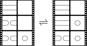
Figure 4.8. Death and saddle chronological movie move

Associated with these movies, we have the following induced maps in each degree $\alpha$.

(91)

(92)

Recall that the chain map assigned to a saddle was defined by considering a larger link diagram. Once we specify an $\alpha$, the saddle that appears in the above maps is either a split or a merge. If the saddle is a split, then the underlying cobordisms $\pi$-commute $\left(\overleftarrow{\varphi}_{1,\alpha}^{2,\alpha}\overleftarrow{\varphi}_{0,\alpha}^{1,\alpha}=\pi\overrightarrow{\varphi}_{1,\alpha}^{2,\alpha}\overrightarrow{\varphi}_{0,\alpha}^{1,\alpha}\right)$. Otherwise, the saddle is a merge and the underlying cobordisms commute $\left(\overleftarrow{\varphi}_{1,\alpha}^{2,\alpha}\overleftarrow{\varphi}_{0,\alpha}^{1,\alpha}=\overrightarrow{\varphi}_{1,\alpha}^{2,\alpha}\overrightarrow{\varphi}_{0,\alpha}^{1,\alpha}\right)$. Note that the saddle maps $\overleftarrow{\Phi}_{1,\alpha}^{2,\alpha}$ and $\overrightarrow{\Phi}_{0,\alpha}^{1,\alpha}$ are built off of essentially the same cube, whence $\overleftarrow{\epsilon}_{1,\alpha}^{2,\alpha}=\overrightarrow{\epsilon}_{0,\alpha}^{1,\alpha}$. To see the change in the powers of $\pi$ appearing in the death maps, we must study the difference $S(\overrightarrow{L}_{1},\alpha)-S(\overleftarrow{L}_{0},\alpha)$. Recalling the definition of the $S$-map, it is easy to see that this difference takes the following values, depending on whether the saddle is a split or a merge on the resolution $\alpha$ and on the all-zero resolution $\zeta$:

$S(\overrightarrow{L}_{1},\alpha)-S(\overleftarrow{L}_{0},\alpha)$	split saddle on $\alpha$	merge saddle on $\alpha$
split saddle on $\zeta$	1	0
merge saddle on $\zeta$	0	$-1$

In summary, we see that, regardless of a choice of $\alpha$, if the saddle is a split with respect to $\zeta$, then $\overleftarrow{\Phi}_{1,\alpha}^{2,\alpha}\overleftarrow{\Phi}_{0,\alpha}^{1,\alpha}=\overrightarrow{\Phi}_{1,\alpha}^{2,\alpha}\overrightarrow{\Phi}_{0,\alpha}^{1,\alpha}$, and if the saddle is a merge with respect to $\zeta$, then $\overleftarrow{\Phi}_{1,\alpha}^{2,\alpha}\overleftarrow{\Phi}_{0,\alpha}^{1,\alpha}=\pi\overrightarrow{\Phi}_{1,\alpha}^{2,\alpha}\overrightarrow{\Phi}_{0,\alpha}^{1,\alpha}$. ∎

4.4.6   Commuting Deaths with Reidemeister I Type Cobordisms

We will show that the inverse Reidemeister I maps $\pi$-commute with death map. Since the Reidemeister I maps are homotopy equivalences, this will imply that the forward versions of these maps also $\pi$-commute with death maps, up to homotopies.

We will first consider inverse positive Reidemeister I maps. Specifically, consider the nonzero portion of the following chain maps. The chain map $\overleftarrow{\Phi}$ is induced by an inverse positive Reidemeister I type cobordism followed by a distant death cobordism. The chain map $\overrightarrow{\Phi}$ is induced by a death cobordism followed by an inverse positive Reidemeister I type cobordism.

(93)

(94)

The underlying cobordisms in the above chain maps $\pi$-commute as both maps contain a single death cobordism. On the left-hand side, the additional powers of $\pi$ cancel as the same power of $\pi$ is applied to both terms. On the right-hand side, $deg(\alpha)$ contributes the same to both $S(\overrightarrow{L}_{0},0\alpha)$ and $S(\overrightarrow{L}_{2},\alpha)$. Moreover, the diagram $\overrightarrow{L}_{2}$ has two fewer circles than $\overrightarrow{L}_{0}$ in both the all-zero resolution and the resolution $\alpha$, so that $S(\overrightarrow{L}_{2},\alpha)=S(\overrightarrow{L}_{0},0\alpha)-2$. Thus, in total $\overleftarrow{\Phi}=\pi\overrightarrow{\Phi}$.

For inverse negative Reidemeister I maps, the argument is almost the same. The difference is that now the underlying cobordisms properly commute with planar death cobordisms, and that the negative Reidemeister I map does not involve powers of $\pi$. In addition, $S(\overrightarrow{L}_{0},0\alpha)$ is replaced by $S(\overrightarrow{L}_{0},1\alpha)$, because the nonzero components of the negative Reidemeister I map are supported in the 1-resolution of the crossing involved in the Reidemeister move. As a result, the overall change in the power of $\pi$ is determined by $S(\overrightarrow{L}_{0},1\alpha)-S(\overleftarrow{L}_{1},\alpha)$, which in this case can be seen to be equal to $1$. Thus, we again have $\overleftarrow{\Phi}=\pi\overrightarrow{\Phi}$.

4.4.7   Commuting Deaths with Reidemeister II Type Cobordisms

Commutativity of deaths with Reidemeister II type cobordisms could be shown by using the same argument that we used to prove the Claim 1 in the proof of Lemma 13. We will instead present a different argument that we can later extend to Reidemeister III type cobordisms. As with Reidemeister I chain maps, its enough to show that either the Reidemeister II chain map or its homotopy inverse commutes with death chain maps. For concreteness, we will focus on the inverse Reidemeister II chain map.

Recall that the components of this chain map are given by two types of planar cobordisms: identity cobordisms and death-and-saddle cobordisms. We will first show that the components containing deaths and saddles commute with the components of the death chain map, up to a possible global factor of $\pi$. For a fixed $\alpha$, the relevant compositions are shown below, where the scalar $\epsilon_{\alpha}$ is the same on both sides.

(95)

(96)

If the saddle is a merge, then the death-and-saddle cobordism has odd superdegree, and hence it $\pi$-commutes with the planar death cobordism that appears in the death chain map. Otherwise, the saddle is a split, and the two planar cobordisms commute because now the death-and-saddle cobordism has even superdegree. To study the relative powers of $\pi$ that show up in the death chain maps, note that

$$S(\overrightarrow{L}_{1},\alpha)-S(\overleftarrow{L}_{0},01\alpha)=a+b$$

where

$$a:=\frac{c(\overrightarrow{L}_{1},\alpha)-c(\overleftarrow{L}_{0},01\alpha)}{2}\qquad\mbox{and}\qquad b:=\frac{c(\overrightarrow{L}_{1},\zeta)-c(\overleftarrow{L}_{0},00\zeta)-1}{2}.$$

If the saddle is a merge, then $a=-1$, as both the death and the merge decrease the number of circles by one. Meanwhile, if the saddle is a split, then $a=0$, as the number of circles is maintained. It follows that $\pi^{a}$ is equal to $\pi$ precisely when the saddle is a merge—i.e., precisely when the underlying planar cobordisms $\pi$-commute. Thus, the death-and-saddle-components of the inverse Reidemeister II chain map pick up a (global) net factor of $\pi^{b}$ when they are commuted past a component of the death chain map. The same result also holds for the identity-components of the inverse Reidemeister II chain map. Indeed, every identity cobordism commutes with planar death cobordisms, and since every identity cobordism maintains the number of circles, the quantity denoted $a$ in the corresponding sum $a+b$ is equal to zero.

4.4.8   Commuting Deaths with Reidemeister III Type Cobordisms

The proof of commtuativity with Reidemeister III Type cobordisms is an extension of the previous proof. Specifically, all components of the Reidemeister III chain map are compositions of the following elementary maps: identity maps, components of Reidemeister II type chain maps, components of differentials, and components of homotopies coming from the proof of Reidemeister II invariance. Suppose $F\colon D_{\alpha}\rightarrow D^{\prime}_{\beta}$ is one of the elementary components just described, where $D_{\alpha}$ and $D^{\prime}_{\beta}$ are two resolutions. We wish to show that $F$ commutes with the components of the death chain map, up to a global power of $\pi$.

To see this, we note that when computing the difference between the $S$-maps associated with $D_{\alpha}$ and $D^{\prime}_{\beta}$, we can replace $deg(\alpha)$ and $deg(\beta)$ by the corresponding homological degrees, from which they differ by global shifts. We can likewise ignore any contributions coming from the all-zero resolutions, as these, too, result in global shifts. The relevant quantity that needs to be considered is thus

$$\Delta(F):=\frac{c(D^{\prime}_{\beta})-c(D_{\alpha})+\sigma(F)}{2}$$

where $c(D^{\prime}_{\beta})$ and $c(D_{\alpha})$ denote the numbers of circles in $D^{\prime}_{\beta}$ and $D_{\alpha}$, respectively, and $\sigma(F)$ is equal to $1$, $0$, or $-1$, depending on whether $F$ is a component of a differential, a chain map, or a homotopy. It is now easy to verify that, for each of the elementary components described before, $\Delta(F)$ is congruent to $1$ modulo $2$ precisely when the planar cobordism underlying $F$ has odd superdegree. Indeed, for components of Reidemeister II chain maps and identity chain maps, this was already shown before, and for components of differentials, this follows from the construction of the $S$-map. Moreover, for components of homotopies, this holds because it holds for the components of the corresponding chain maps and differentials. Arguing as we did for the Reidemeister II chain map, we now conclude that the components of the Reidemeister III chain map commute with the ones of the death chain map, up to a possible global factor of $\pi$.

4.4.9   Commuting a Pair of Saddle Cobordisms

We will show that commuting two saddle cobordisms induces an overall sign. Consider the odd Khovanov bracket of the larger link with two additional crossings corresponding with the two saddles. If we fix a resolution of outside crossings, then the square corresponding with the resolution of the two distinguished vertices anticommutes:

(97) $$\Psi_{{\star}1\alpha}\Psi_{0{\star}\alpha}=-\Psi_{1{\star}\alpha}\Psi_{{\star}0\alpha}$$

The two ways we travel around the face correspond with the rearrangement of the saddles’ order. To produce the final saddle chain maps, we need to multiply by signs on odd degrees so that the maps commute with the differentials.

(98)

This yields the following equation.

(99) $$\begin{split}\overleftarrow{\Phi}_{1,\alpha}^{2,\alpha}\overleftarrow{\Phi}_{0,\alpha}^{1,\alpha}&=(-1)^{\deg(\alpha)}\Psi_{{\star}1\alpha}(-1)^{\deg(\alpha)}\Psi_{0{\star}\alpha}\\ &=-\left[(-1)^{\deg(\alpha)}\Psi_{1{\star}\alpha}(-1)^{\deg(\alpha)}\Psi_{{\star}0\alpha}\right]\\ &=-\overrightarrow{\Phi}_{1,\alpha}^{2,\alpha}\overrightarrow{\Phi}_{0,\alpha}^{1,\alpha}\end{split}$$

Therefore, generally for commuting two saddle cobordisms, $\overleftarrow{\Phi}=-\overrightarrow{\Phi}$.

4.4.10   Commuting Saddles with Reidemeister Type Cobordisms

Will show that a saddle chain map and a Reidemeister chain map commute or anticommute. Consider the larger link diagram $L$ with an additional crossing corresponding to the saddle. Then look at the map on the Khovanov bracket given by performing the Reidemeister move on $L$, yielding a new larger link diagram $L^{\prime}$. Since this map is a chain map, it intertwines with the differentials in $\llbracket L\rrbracket$ and $\llbracket L^{\prime}\rrbracket$, and hence with the components of these differentials that correspond to the saddle maps. The actual saddle maps are obtained from these components by multiplying by prefactors of the form $(-1)^{deg(\alpha)}$ and $(-1)^{deg(\beta)}$, where $\alpha$ and $\beta$ denote indices of vertices in (layers of) the cubes of $L$ and $L^{\prime}$. The main observation is now that the components of the Reidemeister chain map preserve the homological degree, and thus preserve $deg(\alpha)$ up to an overall shift. In the relevant calculations, we can therefore assume that $deg(\beta)=deg(\alpha)+c$ for an overall constant $c$. It follows that the Reidemeister chain map commutes with the saddle chain map if $c$ is even and anticommutes otherwise.

4.4.11   Commuting a Pair of Reidemeister Type Cobordisms

We are left to show that changing the chronological order of a pair of distant Reidemeister type cobordisms at most incurs an overall factor of $\pm 1$ or $\pm\pi$. Let $F$ and $G$ be two cobordisms arising from Reidemeister moves performed in disjoint disks $D_{F}$ and $D_{G}$. Further, let $L$ be the initial link diagram for these cobordisms. We first observe the following.

Lemma 15.

Let $x_{F}$ and $x_{G}$ be distinguished points on the boundaries of $D_{F}$ and $D_{G}$ away from the strands of $L$. There exists a disk $D\subset\mathbb{R}^{2}$ containing both $D_{F}$ and $D_{G}$ such that $\partial D_{F}\cup\partial D_{G}$ is contained in $\partial D$ except for arbitrarily small neighborhoods around the distinguished points, and such that the tangle $L\cap D$ differs from $L\cap(D_{F}\cup D_{G})$ by adding finitely many extra strands and no extra crossings.

Proof.

Choose a non-self-intersecting path $p\subset\mathbb{R}^{2}$ from $x_{F}$ to $x_{G}$ that avoids the crossings of $L$ and meets $D_{F}$ and $D_{G}$ only at its endpoints, and that intersects $L$ transversely at finitely many places. The desired disk $D$ is then given by $D=D_{F}\cup D_{G}\cup P$, where $P\subset\mathbb{R}^{2}$ is a narrow band obtained by thickening $p$. ∎

Depending on the Reidemeister move performed on each of the disks $D_{F}$ and $D_{G}$, we will now choose the points $x_{F}$ and $x_{G}$ on the boundaries of $D_{F}$ and $D_{G}$ according to the rules of acceptable point placement shown in Figure 4.9.

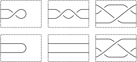
Figure 4.9. The ticked boundary indicates where the path should connect to the disk containing each Reidemeister move

Let $D$ be the larger disk produced by applying the Lemma 15 to our link diagram $L$ with the disks $D_{F}$ and $D_{G}$ and the chosen points $x_{F}$ and $x_{G}$. We have ostensibly dug a tunnel from the disk containing the tangle $L\cap D_{F}$ to the disk containing the tangle $L\cap D_{G}$ in order to produce a single larger tangle $T:=L\cap D$. Consider the commutator of cobordisms $H\coloneqq FGF^{-1}G^{-1}$, which begins and ends at identical diagrams, and which is nontrivial only above $D$. The tangle $T$ satisfies the assumptions of Lemma 13, and thus this lemma implies that $H$ induces a chain map homotopic to $\pm\textnormal{id}$ or $\pm\pi\textnormal{id}$. It follows that either order of composing $F$ and $G$ produces homotopic chain maps up to a global invertible scalar.

5   Non-invariance in $S^{3}\times I$

In this section, we prove Theorem 3 by giving a family of examples showing that the odd cobordism maps are not invariant under smooth ambient isotopies in $S^{3}\times I$. As mentioned in the introduction, the same examples will also show that the odd cobordism maps are not invariant under ribbon moves.

Following [Kan22], let $U_{2}=A\sqcup B$ denote a 2-component unlink consisting of an inner component $A$ and an outer component $B$, and let $D_{1}$ and $D_{2}$ be the disks shown below.

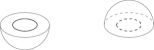
Figure 5.1. The disks $D_{1}$ and $D_{2}$ on the left and right respectively

Note that each of these disks is disjoint from $A$, and can thus be viewed as a Seifert surface for $B$ in $S^{3}\setminus A$. As such, the disks $D_{1}$ and $D_{2}$ are ambient isotopic because we can transform one into the other by pushing it through the point $\infty\in S^{3}$. By pushing the interior of each disk into the 4th dimension, we can further regard $D_{1}$ and $D_{2}$ as link cobordisms $\emptyset\rightarrow B$, and adding the identity cobordism of $A$, we obtain link cobordisms $F_{1},F_{2}\colon A\rightarrow U_{2}$. These cobordisms are still ambient isotopic in $S^{3}\times I$, but we claim that they induce different maps on odd Khovanov homology.

To see this, note that $F_{1}$ and $F_{2}$ are represented by the following movies:

Figure 5.2. The cobordisms $F_{1}$ and $F_{2}$ on the left and right respectively

The first half of each movie is given by the birth of a new component, whereas in the second half, this component is moved over or under the other component (so that the two components switch places). Using notation from [ORS13], the odd Khovanov homology groups of $A$ and $U_{2}$ are given by $OKh(A)=\operatorname{Span}\{1,A\}$ and $OKh(U_{2})=\operatorname{Span}\{1,A,B,A\wedge B\}$. A direct calculation now shows that the maps

$$OKh(A)\longrightarrow OKh(U_{2})$$

induced by $F_{1}$ and $F_{2}$ are given by

$$1\mapsto 1,\qquad A\mapsto A\pm(A-B)$$

where the sign denoted $\pm$ is different for $F_{1}$ and $F_{2}$, and where we are ignoring possible overall signs. On the generator $A$, the values of the two maps thus differ by $\pm 2(A-B)\neq 0$ or by $\pm 2A\neq 0$, depending on whether the overall signs are assumed to be the same or different.

We can easily generalize this example to obtain an infinite family of link cobordisms, as described in Theorem 3. To this end, let $R\colon U_{2}\rightarrow U_{2}$ be the link cobordism $R=R_{2}\circ R_{1}^{-1}$, where the cobordisms $R_{1}$ and $R_{2}$ are given by the second halves of the movies of $F_{1}$ and $F_{2}$, respectively. Then the cobordisms $F_{n}:=R^{(n-1)}\circ F_{1}$ are all ambient isotopic in $S^{3}\times I$, but the maps that they induce on odd Khovanov homology are different since they are given by

$$1\mapsto 1,\qquad A\mapsto A+(3-2n)(A-B)$$

(the computations are left the reader since a conceptual interpretation of the above formulas will be given in [MWa]).

References

- [BHL19] John Baldwin, Matt Hedden and Andrew Lobb “On the functoriality of Khovanov–Floer theories” In Advances in Mathematics 345, 2019, pp. 1162–1205
- [BN02] Dror Bar-Natan “On Khovanov’s categorification of the Jones polynomial” In Algebraic & Geometric Topology, 2002, pp. 2–16
- [BN05] Dror Bar-Natan “Khovanov’s homology for tangles and cobordisms” In Geometry & Topology 9.3 Mathematical Sciences Publishers, 2005, pp. 1443–1499 DOI: 10.2140/gt.2005.9.1443
- [BW10] Anna Beliakova and Emmanuel Wagner “On link homology theories from extended cobordisms” In Quantum Topology 1, 2010, pp. 379–398
- [Bel+23] Anna Beliakova, Matthew Hogancamp, Krzysztof K Putyra and Stephan M Wehrli “On the functoriality of tangle homology” In Algebraic & Geometric Topology 23.3 Mathematical Sciences Publishers, 2023, pp. 1303–1361
- [Bla10] Christian Blanchet “An oriented model for Khovanov homology” In Journal of Knot Theory and Its Ramifications 19.02 World Scientific Pub Co Pte Ltd, 2010, pp. 291–312
- [Cap07] Carmen Caprau “An tangle homology and seamed cobordisms”, 2007 arXiv:0707.3051
- [CS91] J. Scott Carter and Masahico Saito “Syzygies among elementary string interactions in 2+1 dimensions” In Letters in Mathematical Physics 23, 1991, pp. 287–300
- [CS93] J. Scott Carter and Masahico Saito “Reidemeister moves for surface isotopies and their interpretation as moves to movies” In Journal of Knot Theory and Its Ramifications 02.03, 1993, pp. 251–284
- [CS97] J. Scott Carter and Masahico Saito “Knotted Surfaces and Their Diagrams” American Mathematical Society, 1997
- [CSS06] Scott Carter, Masahico Saito and Shin Satoh “Ribbon-moves for 2-knots with 1-handles attached and Khovanov-Jacobsson numbers” In Proc. Amer. Math. Soc. 134, 2006, pp. 2779–2783
- [CMW09] David Clark, Scott Morrison and Kevin Walker “Fixing the functoriality of Khovanov homology” In Geometry & Topology 13.3 Mathematical Sciences Publishers, 2009, pp. 1499–1582
- [EK10] Ben Elias and Dan Krasner “Rouquier complexes are functorial over braid cobordisms” In Homology, Homotopy and Applications 12, 2010, pp. 109–146
- [GLW17] J. Elisenda Grigsby, Anthony M. Licata and Stephan M. Wehrli “Annular Khovanov homology and knotted Schur–Weyl representations” In Compositio Mathematica 154.3 Wiley, 2017, pp. 459–502 DOI: 10.1112/s0010437x17007540
- [HS22] Kyle Hayden and Isaac Sundberg “Khovanov homology and exotic surfaces in the 4-ball”, 2022 arXiv:2108.04810
- [Jac04] Magnus Jacobsson “An invariant of link cobordisms from Khovanov homology” In Algebraic & Geometric Topology 4.2 Mathematical Sciences Publishers, 2004, pp. 1211–1251 DOI: 10.2140/agt.2004.4.1211
- [Jon85] Vaughan F. R. Jones “A polynomial invariant for knots via von Neumann algebras” In Bulletin (New Series) of the American Mathematical Society 12.1 American Mathematical Society, 1985, pp. 103 –111
- [Kan22] Sungkyung Kang “Link homology theories and ribbon concordances” In Quantum Topology 13, 2022, pp. 183–205
- [Kho99] Mikhail Khovanov “A categorification of the Jones polynomial” In Duke Mathematical Journal 101, 1999, pp. 359–426 URL: https://api.semanticscholar.org/CorpusID:119585149
- [KR08] Mikhail Khovanov and Lev Rozansky “Matrix factorizations and link homology” In Fundamenta Mathematicae 199, 2008, pp. 1–91
- [Lee05] Eun Soo Lee “An endomorphism on the Khovanov invariant” In Advances in Mathematics 197, 2005, pp. 554–586
- [LZ19] Adam Simon Levine and Ian Zemke “Khovanov homology and ribbon concordances” In Bulletin of the London Mathematical Society 51.6 Wiley, 2019, pp. 1099–1103 DOI: 10.1112/blms.12303
- [Man14] Andrew Manion “A sign assignment in totally twisted Khovanov homology” In Algebraic & Geometric Topology 14.2 Mathematical Sciences Publishers, 2014, pp. 753–767 DOI: 10.2140/agt.2014.14.753
- [MW] Jacob Migdail and Stephan Wehrli “A module structure on odd Khovanov homology and the odd invariant for ribbon 2-knots” in preparation
- [MWa] Jacob Migdail and Stephan Wehrli “An action of the Hecke algebra on the odd Khovanov homology of certain cables” in preparation
- [MWW22] Scott Morrison, Kevin Walker and Paul Wedrich “Invariants of 4-manifolds from Khovanov-Rozansky link homology” In Geometry & Topology 26, 2022, pp. 3367–3420
- [NP20] Grégoire Naisse and Krzysztof Putyra “Odd Khovanov homology for tangles”, 2020 eprint: arxiv:2003.14290
- [Oga00] Eiji Ogasa “Ribbon-moves of 2-knots: the Farber-Levine pairing and the Atiyah-Patodi-Singer-Casson-Gordon-Ruberman -invariants of 2-knots”, 2000 eprint: arxiv:0004007
- [ORS13] P. S. Ozsváth, Jacob Rasmussen and Zoltán Szabó “Odd Khovanov homology” In Algebraic & Geometric Topology 13.3 Mathematical Sciences Publishers, 2013, pp. 1465–1488 DOI: 10.2140/agt.2013.13.1465
- [OS04] Peter Ozsváth and Zoltán Szabó “Holomorphic disks and topological invariants for closed three-manifolds” In Annals of Mathematics 159, 2004, pp. 1027–1158
- [Pic20] Lisa Piccirillo “The Conway knot is not slice” In Annals of Mathematics 191.2 Department of Mathematics of Princeton University, 2020, pp. 581 –591 DOI: 10.4007/annals.2020.191.2.5
- [PL16] Krzysztof Putyra and Wojciech Lubawski “Mirror links have dual odd and generalized Khovanov homology” In Algebraic & Geometric Topology 16.4 Mathematical Sciences Publishers, 2016, pp. 2021–2044 DOI: 10.2140/agt.2016.16.2021
- [Put13] Krzysztof Karol Putyra “A 2-category of chronological cobordisms and odd Khovanov homology” In Banach Center Publications 103, 2013, pp. 291–355 DOI: 10.4064/bc103-0-12
- [Ras04] Jacob Rasmussen “Khovanov homology and the slice genus” In Inventiones mathematicae 182, 2004, pp. 419–447 URL: https://api.semanticscholar.org/CorpusID:14442088
- [Ras05] Jacob Rasmussen “Khovanov’s invariant for closed surfaces”, 2005 eprint: arxiv:0502527
- [Sal18] Adam Saltz “Strong Khovanov-Floer Theories and Functoriality”, 2018 arXiv: https://arxiv.org/abs/1712.08272
- [San21] Taketo Sano “Fixing the functoriality of Khovanov homology: A simple approach” In Journal of Knot Theory and Its Ramifications 30.11 World Scientific Pub Co Pte Ltd, 2021
- [SV23] Léo Schelstraete and Pedro Vaz “Odd Khovanov homology and higher representation theory”, 2023 arXiv: https://arxiv.org/abs/2311.14394
- [Shu11] Alexander N. Shumakovitch “Patterns in odd Khovanov homology” In Journal of Knot Theory and Its Ramifications 20.1, 2011, pp. 203–222
- [Spy24] Dean Spyropoulos “Jones-Wenzl projectors and odd Khovanov homology”, 2024 arXiv: https://arxiv.org/abs/2410.09269
- [Tan06] Kokoro Tanaka “Khovanov-Jacobsson numbers and invariants of surface knots derived from Bar-Natan’s theory” In Proc. Amer. Math. Soc. 134, 2006
- [Vog20] Pierre Vogel “Functoriality of Khovanov homology” In Journal of Knot Theory and Its Ramifications 29.04 World Scientific Pub Co Pte Ltd, 2020