Continuous Risk Factor Models: Analyzing Asset Correlations through Energy Distance

Abstract

This paper introduces a novel approach to financial risk analysis that does not rely on traditional price and market data, instead using market news to model assets as distributions over a metric space of risk factors. By representing asset returns as integrals over the scalar field of these risk factors, we derive the covariance structure between asset returns. Utilizing encoder-only language models to embed this news data, we explore the relationships between asset return distributions through the concept of Energy Distance, establishing connections between distributional differences and excess returns co-movements. This data-agnostic approach provides new insights into portfolio diversification, risk management, and the construction of hedging strategies. Our findings have significant implications for both theoretical finance and practical risk management, offering a more robust framework for modelling complex financial systems without depending on conventional market data.

I Introduction

In finance, professional and industry standards support a structured approach to risk management, emphasizing the identification and systematic management of diverse risk factors. Through frameworks like ISO 31000, ERM, CFA Standard II(A), and COSO, risk is seen as a mixture of factors that can be systematically identified and managed through diversification, hedging, and other risk management strategies (CFA Institute,, 2017). The Capital Asset Pricing Model (CAPM), Arbitrage Pricing Theory (APT) and multifactor models formalize this idea by positing that asset prices exist as linear combinations of risk factors, each with a corresponding risk premium (Daniel and Titman,, 1997, Fama and French,, 1996, Ross,, 1976). While APT makes no argument regarding the causal, semantic or hierarchical relationships between these factors, this paper looks to explore the role of uncertainty or allocation decisions over semantically related risk factors and itś implications for excess return co-movements. .

I-A Literature Review

Spatial Arbitrage Pricing Theory (sAPT) has been employed extensively in Financial Econometrics to model spatial interaction or spatial correlation between assets, using:

$$R_{i}-R_{f}=\rho_{i}\sum_{j\neq i}^{N}w_{i,j}(R_{j}-R_{f})+\beta_{i}(R_{m}-R_{f})+\sum_{f=1}^{F}\lambda_{f}F_{f}+\epsilon_{i}$$ (1)

where:

• $R_{i}$ represents the return of asset $i$,

• $w_{i,j}$ represents the influence of asset $j$ on asset $i$ based on their spatial proximity or economic interaction based on parameter $\rho_{i}$,

• $\beta_{i}$ is the sensitivity of asset $i$ to the market return $R_{m}$,

• $\lambda_{f}$ represents the exposure to factor mimicking portfolio $f$, $F_{f}$ is the return of factor mimicking portfolio $f$,

• $\rho_{i,j}$ captures the degree of interaction between assets $i$ and $j$, which can be influenced by various spatial or economic factors, and

• $\epsilon_{i}$ is an idiosyncratic error term.

While authors like Fernandez, (2011) have demonstrated the potential of applying sAPT to accounting and financial metrics, Kou et al., (2018) and Bera et al., (2016) extended sAPT to a geographic feature space, using spatial econometric techniques to quantify how local economic conditions allow risk to propagate among geographically neighboring assets. Building on studies by Menzly and Ozbas, (2010) on return comovements across industry-level supplier networks, research by Scherbina and Schlusche, (2013), Schwenkler and Zheng, (2020), and Ge et al., (2023) have used the theoretical foundations in sAPT to characterise excess return contagion across networks of article co-mentions.

While both the geographic and network approaches rely on sAPT, they offer different explanations for the causal structure of risk in financial markets. Authors like Kou et al., (2018) and Bera et al., (2016) suggest that risk emerges from spatial interactions between assets or from shared economic factors tied to specific geographies. In contrast, studies employing network econometrics argue that links between firms facilitate the contagion of risks across the market through the business alliances, partnerships, banking and financing, customer-supplier, and production similarity relationships mentioned in these business articles.

The role of news sentiment in finance has been extensively explored, with research showing its significant impact on market dynamics and stock prices (Tetlock,, 2007, Garcıa,, 2013). While these studies have relied on hand-crafted rules and sentiment dictionaries, more recent works in the field Natural Language Processing (NLP) have posited the benefits of Unsupervised and Self-Supervised Deep Learning-based methods in modelling sentiment Radford et al., (2017). Building on this work, many researchers, including Peng et al., (2021), Pei and Zhang, (2021), Chopra and Ghosh, (2021), Desola et al., (2019) and Araci, (2019), have all contributed language models fine-tuned on financial corpora aimed at tasks in sentiment analysis, returns forecasting, and hypernym classification (Isma¨ıl et al.,, 2020, Mansar et al.,, 2021, Kang et al.,, 2021, Bordea et al.,, 2016).

The literature presents a dichotomy between spatial and network approaches to understanding risk propagation in financial markets. While spatial econometric models, such as sAPT, emphasize geographic and regional economic linkages, network econometrics highlights risk contagion through firm-level relationships, such as business alliances or supply chains. Despite their differences, both approaches face limitations in capturing the full complexity of risk dynamics, particularly when overlooking semantic content in news articles or treating assets as static points in space rather than distributions influenced by multifaceted operations and market conditions.

Our research aims to bridge these perspectives by introducing a new approach that leverages Energy Distances to model covariances in excess returns. By considering firms as distributions in embedding space and incorporating the semantic content of firm-specific news through Semantic Textual Similarity, we provide a richer characterization of economic risk factors and their interrelationships. This approach allows us to constrain and quantify excess return co-movements more effectively, integrating both spatial and network insights while accounting for a broader spectrum of material risk factors, which may include Environmental, Social and Governenance (ESG), sentiment, and operational risks. In doing so, our work contributes to a more nuanced understanding of risk propagation, enhancing opportunities for risk management and portfolio optimization.

In Section II, we present our model and leverage the properties of the Energy Distance to derive constraints on the covariances of excess returns, forming the basis of our hypothesis. In Section III, we test this hypothesis by analyzing financial news data using encoder-only language models, followed by a post-hoc analysis that provides interpretive insights into the results. Lastly, in Section IV, we discuss the broader implications of our findings for financial risk management, emphasizing their potential applications in enhancing risk assessment, improving portfolio diversification, and informing decision-making processes.

II A Continuous Space of Risk Factors

In this paper, we depart from the assumption in sAPT that exists as points in a scalar field of risk factors, and instead consider assets as distributions over this space. This allows us to model the return of an asset as an integral over the risk factor space, capturing the asset’s sensitivity to different risk factors.

Mathematically, this concept can be formalized by representing the random excess return $\tilde{R_{i}}$ of asset $i$ as an integral over a continuous risk factor space $\Omega$:

$$\tilde{R_{i,t}}=\int_{\Omega}\beta_{i}(\omega)\lambda_{t}(\omega)d\omega+\epsilon_{i,t}$$ (2)

where:

• $\tilde{R_{i,t}}$ is $R_{i,t}-r_{f}$, the excess return of asset $i$ over the risk-free rate at time $t$.

• $\beta_{i}(\omega)$ is a valid probability density function that captures the sensitivity (factor loading) of asset $i$ to the risk factor at point $\omega$ in the risk factor space.

• $\lambda_{t}(\omega)$ is the market risk premium associated with risk factor $\omega$ at time $t$, and may be expressed as $\lambda(\omega,t)$ to emphasize its time-varying nature.

• $\Omega$ represents the entire continuous spectrum of risk factors.

• $\omega$ denotes a specific point within the risk factor space.

• $\epsilon_{i,t}$ is the idiosyncratic component of asset $i$’s return at time $t$.

Figure 1: Risk Factor Space $\Omega$ with $\lambda_{t}(\omega)$ and $\beta_{i}(\omega)$. The color gradient represents the market risk premium $\lambda_{t}(\omega)$, while the dashed contour lines represent the sensitivity functions $\beta_{i}(\omega)$ for two different assets. The integral equation $\tilde{R_{i,t}}=\int_{\Omega}\beta_{i}(\omega)\lambda_{t}(\omega)d\omega+\epsilon_{i,t}$ formalizes how these components interact to determine asset returns.

In this framework, the market risk premium function $\lambda_{t}(\omega)$ is assumed to be smooth. Smoothness can be formalized by the differentiability of $\lambda(\omega,t)$ with respect to both $\omega$ and $t$, ensuring that small changes in either the risk factor $\omega$ or time $t$ result in small corresponding changes in the risk premium. Specifically, $\lambda(\omega,t)\in C^{1}(\Omega\times\mathbb{R}^{+})$, meaning it has continuous first derivatives with respect to both $\omega$ and $t$:

$$\frac{\partial\lambda(\omega,t)}{\partial\omega}\quad\text{and}\quad\frac{\partial\lambda(\omega,t)}{\partial t}$$ (3)

are continuous across $\Omega\times\mathbb{R}^{+}$. This ensures that $\lambda(\omega,t)$ is a smooth function of both the risk factor and time.

II-A Derivation of Covariance between Asset Returns

In order to understand the risk of a portfolio of assets, we need to understand the covariance between the returns of different assets. This allows us to quantify the extent to which the returns of two assets move together, and therefore how diversification can reduce the risk of a portfolio.

Continuing from our previous formulation in equation 2, we consider the covariance between the returns of assets $i$ and $j$ at time $t$. The covariance is defined as:

$$\operatorname{Cov}(\tilde{R_{i,t}},\tilde{R_{j,t}})=E[\tilde{R_{i,t}}\tilde{R_{j,t}}]-E[\tilde{R_{i,t}}]E[\tilde{R_{j,t}}]$$ (4)

Given our earlier expression for the expected return of asset $i$:

$$E[\tilde{R_{i,t}}]=\int_{\Omega}\beta_{i}(\omega)\lambda_{t}(\omega)d\omega,$$ (5)

and similarly for asset $j$:

$$E[\tilde{R_{j,t}}]=\int_{\Omega}\beta_{j}(\omega)\lambda_{t}(\omega)d\omega.$$ (6)

To compute $E[\tilde{R_{i,t}}\tilde{R_{j,t}}]$, we consider the product of the returns:

$$\tilde{R_{i,t}}\tilde{R_{j,t}}=\left(\int_{\Omega}\beta_{i}(\omega)\lambda_{t}(\omega)d\omega\right)\left(\int_{\Omega}\beta_{j}(\omega^{\prime})\lambda_{t}(\omega^{\prime})d\omega^{\prime}\right).$$ (7)

Expanding this expression, we have:

$$\tilde{R_{i,t}}\tilde{R_{j,t}}=\int_{\Omega}\int_{\Omega}\beta_{i}(\omega)\beta_{j}(\omega^{\prime})\lambda_{t}(\omega)\lambda_{t}(\omega^{\prime})d\omega d\omega^{\prime}.$$ (8)

Assuming $\lambda_{t}(\omega)$ is deterministic and thus $\lambda_{t}(\omega)=E[\lambda_{t}(\omega)]$, we get:

$$E[\tilde{R_{i,t}}\tilde{R_{j,t}}]=\int_{\Omega}\int_{\Omega}\beta_{i}(\omega)\beta_{j}(\omega^{\prime})E[\lambda_{t}(\omega)\lambda_{t}(\omega^{\prime})]d\omega d\omega^{\prime}.$$ (9)

Substituting back into the covariance formula:

$$\operatorname{Cov}(\tilde{R_{i,t}},\tilde{R_{j,t}})= \int_{\Omega}\int_{\Omega}\beta_{i}(\omega)\beta_{j}(\omega^{\prime})E[\lambda_{t}(\omega)\lambda_{t}(\omega^{\prime})]d\omega d\omega^{\prime}$$

$$-\left(\int_{\Omega}\beta_{i}(\omega)E[\lambda_{t}(\omega)]d\omega\right)$$

$$\quad\times\left(\int_{\Omega}\beta_{j}(\omega^{\prime})E[\lambda_{t}(\omega^{\prime})]d\omega^{\prime}\right).$$

Recognizing that:

$$E[\lambda_{t}(\omega)\lambda_{t}(\omega^{\prime})]=E[\lambda_{t}(\omega)]E[\lambda_{t}(\omega^{\prime})]+\operatorname{Cov}(\lambda_{t}(\omega),\lambda_{t}(\omega^{\prime})),$$ (10)

we can rewrite the covariance expression as:

$$\operatorname{Cov}(\tilde{R_{i,t}},\tilde{R_{j,t}})= \int_{\Omega}\int_{\Omega}\beta_{i}(\omega)\beta_{j}(\omega^{\prime})\Big{(}E[\lambda_{t}(\omega)]E[\lambda_{t}(\omega^{\prime})]$$

$$\quad+\operatorname{Cov}(\lambda_{t}(\omega),\lambda_{t}(\omega^{\prime}))\Big{)}d\omega d\omega^{\prime}$$

$$-\left(\int_{\Omega}\beta_{i}(\omega)E[\lambda_{t}(\omega)]d\omega\right)$$

$$\quad\times\left(\int_{\Omega}\beta_{j}(\omega^{\prime})E[\lambda_{t}(\omega^{\prime})]d\omega^{\prime}\right).$$

Simplifying, the terms involving the products of expectations cancel out:

$$\operatorname{Cov}(\tilde{R_{i,t}},\tilde{R_{j,t}}) =\int_{\Omega}\int_{\Omega}\beta_{i}(\omega)\beta_{j}(\omega^{\prime})\operatorname{Cov}(\lambda_{t}(\omega),\lambda_{t}(\omega^{\prime}))d\omega d\omega^{\prime}.$$ (11)

This expression demonstrates that the covariance between the returns of assets $i$ and $j$ is a double integral over the risk factor space $\Omega\times\Omega$, weighted by the product of their sensitivity functions $\beta_{i}(\omega)$ and $\beta_{j}(\omega^{\prime})$, and the covariance of the market risk premiums $\lambda_{t}(\omega)$ at different points in the risk factor space.

To further elucidate this relationship, suppose that the market risk premium $\lambda_{t}(\omega)$ exhibits a covariance structure $\sigma_{\lambda}^{2}(\omega,\omega^{\prime})$, such that:

$$\operatorname{Cov}(\lambda_{t}(\omega),\lambda_{t}(\omega^{\prime}))=\sigma_{\lambda}^{2}(\omega,\omega^{\prime}).$$ (12)

Substituting this into our covariance expression, we get:

$$\operatorname{Cov}(\tilde{R_{i,t}},\tilde{R_{j,t}})=\int_{\Omega}\int_{\Omega}\beta_{i}(\omega)\beta_{j}(\omega^{\prime})\sigma_{\lambda}^{2}(\omega,\omega^{\prime})d\omega d\omega^{\prime}.$$ (13)

with the variance of the asset returns given by:

$$\operatorname{Var}(\tilde{R_{i,t}})=\int_{\Omega}\int_{\Omega}\beta_{i}(\omega)\beta_{i}(\omega^{\prime})\sigma_{\lambda}^{2}(\omega,\omega^{\prime})d\omega d\omega^{\prime}.$$ (14)

This result highlights that the covariance between the returns of assets $i$ and $j$ depends on the overlap of their sensitivity functions $\beta_{i}(\omega)$ and $\beta_{j}(\omega)$ weighted by the variance of the risk premiums across the risk factor space, and that the variance of an asset’s return is determined by the overlap of its sensitivity function with itself.

II-B Covariances under a Kernel Approximation

In this section, we derive the covariance between the returns of two assets, $\tilde{R}_{i,t}$ and $\tilde{R}_{j,t}$, within the framework of continuous risk factors and a general kernel function modeling the covariance structure of the market risk premium $\lambda_{t}(\omega)$. Our objective is to show that, under appropriate conditions, the covariance can be expressed as

$$\operatorname{Cov}(\tilde{R}_{i,t},\tilde{R}_{j,t})=\sigma_{\lambda}^{2}\int_{\Omega}\beta_{i}(\omega)\beta_{j}(\omega)\,d\omega+u_{t},$$ (15)

where $\sigma_{\lambda}^{2}$ is a constant representing the variance of the market risk premium at each point $\omega$, $\beta_{i}(\omega)$ and $\beta_{j}(\omega)$ are the sensitivity functions of assets $i$ and $j$ respectively, and $u_{t}$ is a residual term that may be zero or modeled as Gaussian noise.

The general expression for the covariance between the excess returns of assets $i$ and $j$ is given by

$$\operatorname{Cov}(\tilde{R}_{i,t},\tilde{R}_{j,t})=\int_{\Omega}\int_{\Omega}\beta_{i}(\omega)\beta_{j}(\omega^{\prime})\operatorname{Cov}[\lambda_{t}(\omega),\lambda_{t}(\omega^{\prime})]\,d\omega\,d\omega^{\prime},$$ (16)

where $\operatorname{Cov}[\lambda_{t}(\omega),\lambda_{t}(\omega^{\prime})]$ denotes the covariance between the market risk premiums at two points $\omega$ and $\omega^{\prime}$ in the risk factor space $\Omega$.

We model this covariance using a kernel function $f_{t}(\omega,\omega^{\prime})$:

$$\operatorname{Cov}[\lambda_{t}(\omega),\lambda_{t}(\omega^{\prime})]=f_{t}(\omega,\omega^{\prime}),$$ (17)

where $f_{t}(\omega,\omega^{\prime})$ is a continuous, symmetric, and positive semi-definite function. Substituting this into equation (16), we obtain

$$\operatorname{Cov}(\tilde{R}_{i,t},\tilde{R}_{j,t})=\int_{\Omega}\int_{\Omega}\beta_{i}(\omega)\beta_{j}(\omega^{\prime})f_{t}(\omega,\omega^{\prime})\,d\omega\,d\omega^{\prime}.$$ (18)

To simplify this expression, we consider that the kernel function $f_{t}(\omega,\omega^{\prime})$ is dominated by its diagonal terms, i.e., when $\omega=\omega^{\prime}$. This assumption is justified in scenarios where the covariance between $\lambda_{t}(\omega)$ and $\lambda_{t}(\omega^{\prime})$ decreases rapidly as the distance $|\omega-\omega^{\prime}|$ increases, implying that risk factors are significantly correlated only when they are close in the risk factor space.

Under this assumption, we approximate the kernel function as

$$f_{t}(\omega,\omega^{\prime})\approx\sigma_{\lambda}^{2}\delta(\omega-\omega^{\prime}),$$ (19)

where $\delta(\omega-\omega^{\prime})$ is the Dirac delta function, and $\sigma_{\lambda}^{2}$ captures the variance of the market risk premium at each point $\omega$.

Substituting this approximation into equation (18), we have

$$\operatorname{Cov}(\tilde{R}_{i,t},\tilde{R}_{j,t}) \approx\sigma_{\lambda}^{2}\int_{\Omega}\int_{\Omega}\beta_{i}(\omega)\beta_{j}(\omega^{\prime})\delta(\omega-\omega^{\prime})\,d\omega\,d\omega^{\prime}$$

$$=\sigma_{\lambda}^{2}\int_{\Omega}\beta_{i}(\omega)\beta_{j}(\omega)\,d\omega,$$ (20)

where we have used the sifting property of the Dirac delta function:

$$\int_{\Omega}\delta(\omega-\omega^{\prime})g(\omega^{\prime})\,d\omega^{\prime}=g(\omega).$$

Equation (20) matches the desired covariance expression in equation (15) with $u_{t}=0$.

Recognizing that the kernel function may not be exactly a Dirac delta function due to residual covariances between different risk factors, we decompose $f_{t}(\omega,\omega^{\prime})$ into two components:

$$f_{t}(\omega,\omega^{\prime})=\sigma_{\lambda}^{2}\delta(\omega-\omega^{\prime})+\epsilon_{t}(\omega,\omega^{\prime}),$$ (21)

where $\epsilon_{t}(\omega,\omega^{\prime})$ captures the off-diagonal elements representing the residual covariance between different points in $\Omega$.

Substituting this decomposition into equation (18), we obtain

$$\operatorname{Cov}(\tilde{R}_{i,t},\tilde{R}_{j,t}) =\sigma_{\lambda}^{2}\int_{\Omega}\beta_{i}(\omega)\beta_{j}(\omega)\,d\omega+\int_{\Omega}\int_{\Omega}\beta_{i}(\omega)\beta_{j}(\omega^{\prime})\epsilon_{t}(\omega,\omega^{\prime})\,d\omega\,d\omega^{\prime}$$

$$=\sigma_{\lambda}^{2}\int_{\Omega}\beta_{i}(\omega)\beta_{j}(\omega)\,d\omega+u_{t},$$ (22)

where we define the residual term $u_{t}$ as

$$u_{t}=\int_{\Omega}\int_{\Omega}\beta_{i}(\omega)\beta_{j}(\omega^{\prime})\epsilon_{t}(\omega,\omega^{\prime})\,d\omega\,d\omega^{\prime}.$$ (23)

The term $u_{t}$ represents the contribution to the covariance from the residual correlations embodied in $\epsilon_{t}(\omega,\omega^{\prime})$. Depending on the characteristics of $\epsilon_{t}(\omega,\omega^{\prime})$, $u_{t}$ may be negligible or can be modeled as a Gaussian noise term if $\epsilon_{t}(\omega,\omega^{\prime})$ exhibits appropriate stochastic properties.

Thus, under the assumption that the covariance between market risk premiums is predominantly determined by the diagonal terms and that the off-diagonal contributions are captured by $u_{t}$, we derive the covariance expression in equation (15).

This result underscores that the covariance between the excess returns of assets $i$ and $j$ primarily depends on the overlap of their sensitivity functions $\beta_{i}(\omega)$ and $\beta_{j}(\omega)$ across the risk factor space $\Omega$. Assets with sensitivity functions concentrated in similar regions of $\Omega$ will exhibit higher covariance due to their shared exposure to common risk factors.

Understanding this covariance structure has significant implications for portfolio construction and risk management. It suggests that diversification benefits can be achieved by selecting assets with non-overlapping or negatively correlated sensitivity functions, thereby reducing the covariance between their returns. By analyzing the sensitivity functions, portfolio managers can strategically adjust the portfolio’s exposure to different regions in the risk factor space to effectively manage risk and optimize returns.

II-C Correlation between Asset Returns

The Pearson correlation coefficient between the returns of assets $i$ and $j$ at time $t$ is defined as:

$$\operatorname{Corr}(\tilde{R_{i,t}},\tilde{R_{j,t}})=\frac{\operatorname{Cov}(\tilde{R_{i,t}},\tilde{R_{j,t}})}{\sqrt{\operatorname{Var}(\tilde{R_{i,t}})\operatorname{Var}(\tilde{R_{j,t}})}}.$$ (24)

We begin by considering the full covariance structure between $\tilde{R_{i,t}}$ and $\tilde{R_{j,t}}$, which can be expressed as a double integral over the risk factor space $\Omega$:

$$\operatorname{Cov}(\tilde{R_{i,t}},\tilde{R_{j,t}})=\int_{\Omega}\int_{\Omega}\beta_{i}(\omega)\beta_{j}(\omega^{\prime})\operatorname{Cov}[\lambda_{t}(\omega),\lambda_{t}(\omega^{\prime})]d\omega d\omega^{\prime}.$$ (25)

Similarly, the variances of the returns for assets $i$ and $j$ are given by:

$$\operatorname{Var}(\tilde{R_{i,t}})=\int_{\Omega}\int_{\Omega}\beta_{i}(\omega)\beta_{i}(\omega^{\prime})\operatorname{Cov}[\lambda_{t}(\omega),\lambda_{t}(\omega^{\prime})]d\omega d\omega^{\prime},$$ (26)

and

$$\operatorname{Var}(\tilde{R_{j,t}})=\int_{\Omega}\int_{\Omega}\beta_{j}(\omega)\beta_{j}(\omega^{\prime})\operatorname{Cov}[\lambda_{t}(\omega),\lambda_{t}(\omega^{\prime})]d\omega d\omega^{\prime}.$$ (27)

Using a general kernel function $f_{t}(d(\omega,\omega^{\prime}))$, which models the covariance between the market risk premiums at different points $\omega$ and $\omega^{\prime}$ in the risk factor space:

$$\operatorname{Cov}[\lambda_{t}(\omega),\lambda_{t}(\omega^{\prime})]=\sigma_{\lambda}^{2}f_{t}(d(\omega,\omega^{\prime})).$$ (28)

We can now capture how the correlation between risk premiums decays or varies based on the distance $d(\omega,\omega^{\prime})$ between points in the risk factor space. Substituting this into the covariance and variance expressions, we have:

$$\operatorname{Cov}(\tilde{R_{i,t}},\tilde{R_{j,t}})=\sigma_{\lambda}^{2}\int_{\Omega}\int_{\Omega}\beta_{i}(\omega)\beta_{j}(\omega^{\prime})f_{t}(d(\omega,\omega^{\prime}))d\omega d\omega^{\prime},$$ (29)

and

$$\operatorname{Var}(\tilde{R_{i,t}})=\sigma_{\lambda}^{2}\int_{\Omega}\int_{\Omega}\beta_{i}(\omega)\beta_{i}(\omega^{\prime})f_{t}(d(\omega,\omega^{\prime}))d\omega d\omega^{\prime},$$ (30)

$$\operatorname{Var}(\tilde{R_{j,t}})=\sigma_{\lambda}^{2}\int_{\Omega}\int_{\Omega}\beta_{j}(\omega)\beta_{j}(\omega^{\prime})f_{t}(d(\omega,\omega^{\prime}))d\omega d\omega^{\prime}.$$ (31)

Which assuming, either the constant or Dirac delta kernel functions, allows us to collapse the double integrals to:

$$\operatorname{Corr}(\tilde{R_{i,t}},\tilde{R_{j,t}})=\frac{\int_{\Omega}\beta_{i}(\omega)\beta_{j}(\omega)d\omega}{\sqrt{\int_{\Omega}\beta_{i}^{2}(\omega)d\omega\cdot\int_{\Omega}\beta_{j}^{2}(\omega)d\omega}}$$ (32)

Which represents the normalized inner product of the sensitivity functions $\beta_{i}(\omega)$ and $\beta_{j}(\omega)$ in the $L^{2}$ space over $\Omega$.

II-D Special Cases of Divergence and Correlation

In our analysis of asset return correlations within the continuous risk factor framework, we examine three noteworthy special cases: perfect positive correlation, zero correlation and correlation defined through some positive semi-definite kernel. These cases provide valuable insights into the relationship between asset sensitivity functions and their corresponding return correlations.

In the case of perfect correlation, we look to show that $\operatorname{Corr}(\tilde{R_{i,t}},\tilde{R_{j,t}})=1$ if and only if $\beta_{i}(\omega)=\beta_{j}(\omega)$ for all $\omega\in\Omega$. Using the Cauchy-Schwarz inequality:

$$\int_{\Omega}f(\omega)g(\omega),d\omega\leq\sqrt{\int_{\Omega}f^{2}(\omega),d\omega}\cdot\sqrt{\int_{\Omega}g^{2}(\omega),d\omega},$$ (33)

equality holds if and only if $f(\omega)$ and $g(\omega)$ are linearly dependent. In our context, if $\beta_{i}(\omega)=\beta_{j}(\omega)$ for all $\omega\in\Omega$, then:

$$\int_{\Omega}\beta_{i}(\omega)\beta_{j}(\omega),d\omega=\int_{\Omega}\beta_{i}^{2}(\omega),d\omega=\int_{\Omega}\beta_{j}^{2}(\omega),d\omega.$$ (34)

Using this result in the expression for the correlation between the returns simplifies to:

$$\operatorname{Corr}(\tilde{R_{i,t}},\tilde{R_{j,t}})=\frac{\int_{\Omega}\beta_{i}^{2}(\omega),d\omega}{\sqrt{\int_{\Omega}\beta_{i}^{2}(\omega),d\omega\cdot\int_{\Omega}\beta_{i}^{2}(\omega),d\omega}}=1.$$ (35)

If $\operatorname{Corr}(\tilde{R_{i,t}},\tilde{R_{j,t}})=1$, the Cauchy-Schwarz inequality must hold with equality, implying $\beta_{i}(\omega)=c\beta_{j}(\omega)$ for some constant $c$. Given that both $\beta_{i}(\omega)$ and $\beta_{j}(\omega)$ are probability density functions (integrating to 1), it follows that $c=1$, and thus $\beta_{i}(\omega)=\beta_{j}(\omega)$ must hold. Therefore, showing that:

$$\operatorname{Corr}(\tilde{R_{i,t}},\tilde{R_{j,t}})=1\quad\text{if and only if}\quad\beta_{i}(\omega)=\beta_{j}(\omega).$$ (36)

In the case of zero correlation, we adopt an information-theoretic approach using the Kullback-Leibler (KL) divergence. The KL divergence quantifies the dissimilarity between two probability distributions. For our sensitivity functions $\beta_{i}(\omega)$ and $\beta_{j}(\omega)$, the KL divergence is defined as:

$$D_{KL}(\beta_{i}\parallel\beta_{j})=\int_{\Omega}\beta_{i}(\omega)\log\left(\frac{\beta_{i}(\omega)}{\beta_{j}(\omega)}\right),d\omega.$$ (37)

When the KL divergence between $\beta_{i}(\omega)$ and $\beta_{j}(\omega)$ approaches infinity, it indicates that the two functions have negligible overlap in the risk factor space. Consequently, the integral:

$$\int_{\Omega}\beta_{i}(\omega)\beta_{j}(\omega),d\omega\to 0$$ (38)

Thus, assuming the Dirac delta function as our kernel function, when the KL divergence is infinite, indicating extreme dissimilarity between $\beta_{i}(\omega)$ and $\beta_{j}(\omega)$, the correlation between the two asset returns must be zero.

II-E The Energy Distance between Risk Factors

To quantify the disparity between the distributions of asset returns in this continuous risk factor framework, we employ the concept of Energy Distance, defined between two random variables with cumulative distribution functions $F_{i}(\omega)$ and $F_{j}(\omega)$ by:

$$D^{2}(F_{i},F_{j})=2\int_{\Omega}(F_{i}(\omega)-F_{j}(\omega))^{2}d\omega,$$ (39)

This metric measures the squared $L_{2}$ distance between the CDFs of the two assets, effectively capturing the distributional differences between them across the continuous risk factor space $\Omega$.

To establish a relationship between the Energy Distance $D^{2}(F_{i},F_{j})$ and the Pearson correlation coefficient $\operatorname{Corr}(\tilde{R_{i,t}},\tilde{R_{j,t}})$, we proceed by expressing the Energy Distance in terms of the differences between the sensitivity functions.

The difference between the CDFs is then:

$$F_{i}(\omega)-F_{j}(\omega)=\int_{-\infty}^{\omega}[\beta_{i}(u)-\beta_{j}(u)]du.$$ (40)

Let us define $h(u)=\beta_{i}(u)-\beta_{j}(u)$ and $H(\omega)=\int_{-\infty}^{\omega}h(u)du$. The Energy Distance becomes:

$$D^{2}(F_{i},F_{j})=2\int_{\Omega}[H(\omega)]^{2}d\omega.$$ (41)

To connect $D^{2}(F_{i},F_{j})$ to the $L^{2}$ norm of $h(u)$, we utilize Parseval’s identity from Fourier analysis, which relates the integral of the square of a function to the integral of the square of its Fourier transform. The Fourier transform of $H(\omega)$ is:

$$\hat{H}(s)=\frac{\hat{h}(s)}{is},$$ (42)

where $\hat{h}(s)$ is the Fourier transform of $h(u)$. Applying Parseval’s identity:

$$\int_{-\infty}^{\infty}|H(\omega)|^{2}d\omega=\int_{-\infty}^{\infty}\left|\frac{\hat{h}(s)}{is}\right|^{2}ds=\int_{-\infty}^{\infty}\frac{|\hat{h}(s)|^{2}}{s^{2}}ds.$$ (43)

Similarly, the $L^{2}$ norm of $h(u)$ is:

$$\int_{-\infty}^{\infty}|h(u)|^{2}du=\int_{-\infty}^{\infty}|\hat{h}(s)|^{2}ds.$$ (44)

Comparing these expressions, we observe that:

$$D^{2}(F_{i},F_{j}) =2\int_{-\infty}^{\infty}\frac{|\hat{h}(s)|^{2}}{s^{2}}ds$$

$$\geq 2\int_{-\infty}^{\infty}|\hat{h}(s)|^{2}ds$$

$$=2\int_{-\infty}^{\infty}|h(u)|^{2}du.$$

This inequality holds because $s^{-2}\geq 0$ for all $s\neq 0$, and it implies that the Energy Distance is at least twice the $L^{2}$ norm of the difference between the sensitivity functions:

$$D^{2}(F_{i},F_{j})\geq 2\int_{\Omega}[\beta_{i}(u)-\beta_{j}(u)]^{2}du.$$ (45)

Next, we examine the Pearson correlation coefficient between the returns $\tilde{R_{i,t}}$ and $\tilde{R_{j,t}}$, given by:

$$\operatorname{Corr}(\tilde{R_{i,t}},\tilde{R_{j,t}})=\frac{\int_{\Omega}\beta_{i}(\omega)\beta_{j}(\omega)d\omega}{\sqrt{\int_{\Omega}\beta_{i}^{2}(\omega)d\omega\cdot\int_{\Omega}\beta_{j}^{2}(\omega)d\omega}}.$$ (46)

To relate this to the $L^{2}$ norm of $h(u)$, we use the identity:

$$\int_{\Omega}\beta_{i}(\omega)\beta_{j}(\omega)d\omega=\frac{1}{2}\Big{(} \int_{\Omega}\beta_{i}^{2}(\omega)d\omega$$

$$+\int_{\Omega}\beta_{j}^{2}(\omega)d\omega$$

$$-\int_{\Omega}[\beta_{i}(\omega)-\beta_{j}(\omega)]^{2}d\omega\Big{)}.$$

This expression shows that as $\int_{\Omega}[\beta_{i}(\omega)-\beta_{j}(\omega)]^{2}d\omega$ increases, the numerator of the correlation coefficient decreases.

Continuing from where we left off, we can establish a more direct relationship between the Energy Distance $D^{2}(F_{i},F_{j})$ and the Pearson correlation coefficient $\operatorname{Corr}(\tilde{R_{i,t}},\tilde{R_{j,t}})$ by expressing both in terms of the integrals of the sensitivity functions $\beta_{i}(\omega)$ and $\beta_{j}(\omega)$.

First, recall the expressions we have derived:

$$D^{2}(F_{i},F_{j})\geq 2\int_{\Omega}[\beta_{i}(\omega)-\beta_{j}(\omega)]^{2}d\omega$$ (47)

and

$$\operatorname{Corr}(\tilde{R_{i,t}},\tilde{R_{j,t}})=\frac{\int_{\Omega}\beta_{i}(\omega)\beta_{j}(\omega)d\omega}{\sqrt{\int_{\Omega}\beta_{i}^{2}(\omega)d\omega\cdot\int_{\Omega}\beta_{j}^{2}(\omega)d\omega}}.$$ (48)

To facilitate the relationship between these two metrics, let’s introduce the following notations:

$$A=\int_{\Omega}\beta_{i}^{2}(\omega)d\omega,\quad B=\int_{\Omega}\beta_{j}^{2}(\omega)d\omega,\quad\text{and}\quad C=\int_{\Omega}\beta_{i}(\omega)\beta_{j}(\omega)d\omega.$$ (49)

With these definitions, the Pearson correlation coefficient can be rewritten as:

$$\operatorname{Corr}(\tilde{R_{i,t}},\tilde{R_{j,t}})=\frac{C}{\sqrt{AB}}.$$ (50)

Next, expand the integral of the squared difference between the sensitivity functions:

$$\int_{\Omega}[\beta_{i}(\omega)-\beta_{j}(\omega)]^{2}d\omega=\int_{\Omega}\beta_{i}^{2}(\omega)d\omega+\int_{\Omega}\beta_{j}^{2}(\omega)d\omega-2\int_{\Omega}\beta_{i}(\omega)\beta_{j}(\omega)d\omega=A+B-2C.$$ (51)

Substituting this into the inequality for the Energy Distance, we obtain:

$$D^{2}(F_{i},F_{j})\geq 2(A+B-2C).$$ (52)

Now, express $C$ in terms of the correlation coefficient:

$$C=\operatorname{Corr}(\tilde{R_{i,t}},\tilde{R_{j,t}})\sqrt{AB}.$$ (53)

Substituting this back into the inequality for $D^{2}(F_{i},F_{j})$:

$$D^{2}(F_{i},F_{j})\geq 2\left(A+B-2\operatorname{Corr}(\tilde{R_{i,t}},\tilde{R_{j,t}})\sqrt{AB}\right).$$ (54)

Thus if $A=B$, then $D^{2}(F_{i},F_{j})=0$ and:

$$0\geq 2\left(A+A-2\operatorname{Corr}(\tilde{R_{i,t}},\tilde{R_{j,t}})\sqrt{AA}\right).$$ (55)

would only hold if and only if $\operatorname{Corr}(\tilde{R_{i,t}},\tilde{R_{j,t}})=1$.

II-F Transforming Correlations under Market Efficiency

In our previous derivations, we assumed that the market risk premiums $\lambda_{t}(\omega)$ are uncorrelated across the risk factor space $\Omega$. In this section, we look to show why under market efficiency, correlations across our scalar field have no impact on the pairwise Energy Distance between assetś sensitivity functions.

Let $T:\Omega\rightarrow\tilde{\Omega}$ be an invertible transformation mapping the original risk factor space $\Omega$ to a new space $\tilde{\Omega}$. In this transformed space, the market risk premiums are defined as $\tilde{\lambda}_{t}(\tilde{\omega})=\lambda_{t}(T^{-1}(\tilde{\omega}))$, and the sensitivity functions become $\tilde{\beta}_{i}(\tilde{\omega})=\beta_{i}(T^{-1}(\tilde{\omega}))\left|\frac{\partial T^{-1}(\tilde{\omega})}{\partial\tilde{\omega}}\right|$, where $\left|\frac{\partial T^{-1}(\tilde{\omega})}{\partial\tilde{\omega}}\right|$ is the determinant of the Jacobian matrix of the inverse transformation. The transformation $T$ is designed such that in $\tilde{\Omega}$, the market risk premiums $\tilde{\lambda}_{t}(\tilde{\omega})$ exhibit high correlations across different points $\tilde{\omega}$, even if $\lambda_{t}(\omega)$ are uncorrelated in $\Omega$. This effectively clusters risk factors into a compressed representation where firms perceive and manage risks at an aggregated level.

In this transformed space, firms optimize their sensitivity functions $\tilde{\beta}_{i}(\tilde{\omega})$ to minimize the variance of their returns for a given expected return. The optimization problem for firm $i$ is formulated as

$$\tilde{\beta}_{i}^{\star}(\tilde{\omega})=\min_{\tilde{\beta}_{i}(\tilde{\omega})}\quad \operatorname{Var}(\tilde{R}_{i,t})+\gamma C\big{(}\tilde{\beta}_{i}(\tilde{\omega}),\tilde{\beta}_{i}^{0}(\tilde{\omega})\big{)}$$ (56)

subject to $$\mathbb{E}[\tilde{R}_{i,t}]=\int_{\tilde{\Omega}}\tilde{\beta}_{i}(\tilde{\omega})\mathbb{E}\big{[}\tilde{\lambda}_{t}(\tilde{\omega})\big{]}\,d\tilde{\omega}=\mu_{i}.$$ (57)

where $\mu_{i}$ is the target expected return of firm $i$, $\tilde{R}_{i,t}$ is the return in the transformed space, and $\gamma C\big{(}\tilde{\beta}_{i}(\tilde{\omega}),\tilde{\beta}_{i}^{0}(\tilde{\omega})\big{)}$ is some penalty function that encourages the sensitivity functions to remain close to an initial endowment sensitivity function $\tilde{\beta}_{i}^{0}(\tilde{\omega})$. The penalty term $C\big{(}\tilde{\beta}_{i}(\tilde{\omega}),\tilde{\beta}_{i}^{0}(\tilde{\omega})\big{)}$ is designed to capture the cost of deviation from an initial endowed sensitivity function, which reflect the cost in changing the firm’s risk exposure profile. This cost exists due to the operational and strategic adjustments required to realign the firm’s operations and risk management practices with the new sensitivity functions.

Under the given optimization, assuming all firms are risk neural and faced with the same cost function under free market conditions, all firms with the same initial endowment sensitivity function $\tilde{\beta}_{i}^{0}(\tilde{\omega})$ will converge to the same sensitivity function $\tilde{\beta}_{i}^{*}(\tilde{\omega})$.

We now consider a scenario involving two firms, Firm A and Firm B as follows:

$$\tilde{\beta}_{A}^{0}(\tilde{\omega})=\alpha\tilde{\beta}_{B}^{0}(\tilde{\omega})+(1-\alpha)\tilde{\beta}_{U}^{0}(\tilde{\omega}),$$

where $0<\alpha<1$, $\tilde{\beta}_{B}^{0}(\tilde{\omega})$ is Firm B’s initial endowment, and $\tilde{\beta}_{U}^{0}(\tilde{\omega})$ is an uncorrelated sensitivity function, satisfying

$$\int_{\tilde{\Omega}}\tilde{\beta}_{B}^{0}(\tilde{\omega})\tilde{\beta}_{U}^{0}(\tilde{\omega})\,d\tilde{\omega}=0,$$

and,

$$Cov[\tilde{R_{B}},\tilde{R_{U}}]=0$$

This formulation ensures that Firm A’s initial endowment is a linear combination of Firm B’s endowment and an entirely uncorrelated component.

As these components are entirely uncorrelated, after optimization the sensivity functions of Firm A will be:

$$\tilde{\beta}_{A}^{\star}(\tilde{\omega})=\alpha^{*}\tilde{\beta}_{B}^{\star}(\tilde{\omega})+(1-\alpha^{*})\tilde{\beta}_{U}^{\star}(\tilde{\omega}),$$

with $\alpha^{*}$ being the new weighting determined under optimization. As the sensitivity functions of Firm A is still a linear combination of Firm B’s and an uncorrelated component, both the distance $D(\tilde{\beta}_{A}(\tilde{\omega}),\tilde{\beta}_{B}(\tilde{\omega}))$ and the correlation $\operatorname{Corr}(\tilde{R_{A}},\tilde{R_{B}})$ will depend only on the weighting $\alpha^{*}$, allowing us to undergo the projection $T^{-1}$ to the space $\Omega$, in which all $\operatorname{Cov}(\lambda_{t}{\omega,\omega^{\prime}})=0$ and the distance between distributions is determined by their mixing parameters $\alpha^{*}$.

III Application

Although asset returns $\tilde{R_{i,t}}$ are observable in financial markets, the variables $\lambda_{t}(\omega)$ (the market price of risk at time $t$ for factor $\omega$), $\beta_{i}(\omega)$ (the sensitivity of asset $i$ to factor $\omega$), and the risk factor space $\Omega$ itself are latent and not directly observable. We do not impose specific functional forms on $\lambda_{t}(\omega)$ or make assumptions about the structure of the risk factor space $\Omega$. Consequently, we do not claim to know the exact distribution of returns in the market. However, by leveraging the framework of Energy Distance, we can develop a statistical test to assess the relationships between asset returns and their underlying risk factors.

We formulate the following null and alternative hypotheses based on the Energy Distance inequality:

$$H_{0}:D^{2}(F_{i},F_{j})<2\left(A+B-2\operatorname{Corr}(\tilde{R_{i,t}},\tilde{R_{j,t}})\sqrt{AB}\right),$$ (58)

$$H_{1}:D^{2}(F_{i},F_{j})\geq 2\left(A+B-2\operatorname{Corr}(\tilde{R_{i,t}},\tilde{R_{j,t}})\sqrt{AB}\right),$$ (59)

where:

• $D^{2}(F_{i},F_{j})$ is the squared Energy Distance between the distributions $F_{i}$ and $F_{j}$ of the latent risk factors for assets $i$ and $j$.

• $A=\int_{\Omega}\beta_{i}^{2}(\omega)d\omega$ and $B=\int_{\Omega}\beta_{j}^{2}(\omega)d\omega$ represent the variances of the sensitivity functions for assets $i$ and $j$, respectively.

• $\operatorname{Corr}(\tilde{R_{i,t}},\tilde{R_{j,t}})$ is the Pearson correlation coefficient between the returns of assets $i$ and $j$.

The Energy Distance $D^{2}(F_{i},F_{j})$ quantifies the disparity between the risk factor distributions of the two assets. The right-hand side of the inequality involves observable quantities derived from asset returns, providing a link between the latent risk factors and observable market data.

To evaluate these hypotheses, we employ Mantel’s one-sided test, which assesses the correlation between two distance matrices (Mantel,, 1967). In our context, the first matrix is based on the Energy Distances between assets, reflecting differences in their latent risk factor distributions. The second matrix is constructed from distances implied by the observed return correlations and variances. The Mantel test statistic is calculated as:

$$Z_{M}=\frac{\sum_{i=1}^{N}\sum_{j=1}^{N}w_{ij}d_{ij}}{\sqrt{\sum_{i=1}^{N}\sum_{j=1}^{N}w_{ij}^{2}\sum_{i=1}^{N}\sum_{j=1}^{N}d_{ij}^{2}}},$$ (60)

where:

• $w_{ij}=D(F_{i},F_{j})$ is the Energy Distance between assets $i$ and $j$.

• $d_{ij}=\sigma_{i}^{2}+\sigma_{j}^{2}-2\operatorname{Corr}(\tilde{R_{i,t}},\tilde{R_{j,t}})\sigma_{i}\sigma_{j}$ represents the distance based on observed returns, with $\sigma_{i}^{2}$ and $\sigma_{j}^{2}$ being the variances of assets $i$ and $j$, respectively.

The p-value is determined through permutation testing, allowing us to assess the statistical significance of the observed association between the two distance matrices.

Using this approach, we look to prove whether the Energy Distance between assets places an upper bound on the correlations between their returns, as predicted by the continuous risk factor framework. Given such a bound, we can infer that assets with more similar distributions in the latent risk factor space exhibit higher correlations in their returns, validating the theoretical foundations of our model, providing insights into the emergence of asset return correlations from underlying risk factors.

III-A Methodology

To estimate the distance between latent risk factors, $d(\omega,\omega^{\prime})$, we utilize the Nomic-Embed-Text-v1 model—a bi-encoder transformer architecture with 137 million parameters designed for generating high-quality text embeddings (Nussbaum et al.,, 2024). This model employs a BERT-style architecture featuring bidirectional attention, rotary positional embeddings, and Flash Attention mechanisms for efficient processing of long sequences (Dao et al.,, 2022, Devlin et al.,, 2019, Su et al.,, 2023). It was pre-trained using a contrastive loss function over 235 million curated text pairs and fine-tuned on tasks aimed at semantic textual similarity. The training corpus includes diverse data sources such as Wikipedia articles, Amazon product reviews, and Reddit discussions, enabling the model to capture rich semantic relationships across various contexts.

For each asset, we aggregate document embeddings derived from news articles related to that asset. The similarity between assets is then measured using the angular distance between their aggregated embeddings:

$$d(\mathbf{u},\mathbf{v})=\frac{1}{\pi}\cos^{-1}\left(\frac{\mathbf{u}\cdot\mathbf{v}}{\|\mathbf{u}\|\|\mathbf{v}\|}\right),$$ (61)

where $\mathbf{u}$ and $\mathbf{v}$ are the aggregated embedding vectors for assets $i$ and $j$, respectively. The angular distance satisfies the triangle inequality, making it a suitable metric for measuring distances in high-dimensional embedding spaces.

Our dataset comprises 66,000 news articles covering 53 companies listed on the Nasdaq, published between 2018 and 2022. These 53 companies are chosen, based on the results in Neto, (2024), to ensure all companies have at least 64 news articles in each year in the sample period and are listed in the Appendix in Subsection .B. These news articles serve as proxies for the latent sensitivity functions $\beta_{i}(\omega)$, under the premise that news content reflects discussion and analysis of information influencing asset sensitivities to underlying risk factors. By capturing the semantic content of the news articles through embeddings, we approximate the distribution of each asset’s sensitivities across the risk factor space.

While bi-encoders offer efficient computation of embeddings, cross-encoders—which jointly encode pairs of documents—could provide more nuanced modeling of relationships between asset pairs. However, due to computational constraints, we focus on bi-encoders in this study.

The embeddings for each asset are aggregated over time to estimate the distribution of $\beta_{i}(\omega)$ across the risk factor space $\Omega$. Specifically, we average the embeddings of all news articles associated with each asset to obtain a representative vector. The angular distances between these aggregated embeddings are then used to compute the Energy Distances required for the Mantel test.

III-B Results

The Mantel test yielded a Mantel correlation coefficient of 0.412 with a corresponding p-value of 0.0001. This significant result allows us to reject the null hypothesis that the Energy Distance between assets does not constrain the observed return correlations. Instead, we find strong evidence supporting the alternative hypothesis that the Energy Distance inequality holds in our data. Specifically, the positive Mantel correlation indicates that assets with more similar distributions in the latent risk factor space—approximated through their aggregated news embeddings—tend to exhibit higher correlations in their returns.

This finding implies that the Energy Distance between assets serves as an upper bound on the correlations between their returns. The relationship suggests that as the similarity between the latent risk factor distributions of two assets increases, the correlation between their returns also tends to increase. This observation holds asymptotically, reinforcing the theoretical underpinnings of our approach.

From a practical standpoint, these results suggest that modelling the semantic content of news articles can provide valuable insights into the covariance structure between assets. By capturing the shared information and market sentiments reflected in news coverage, we can infer significant aspects of how assets co-move in response to underlying risk factors.

This has important implications for financial risk management and portfolio construction. Incorporating latent risk factors derived from textual data can enhance the accuracy of risk forecasts by accounting for information not captured by traditional quantitative models. Additionally, understanding the semantic relationships between assets can inform diversification strategies, helping investors construct portfolios that are better insulated against common sources of risk.

III-C Post-hoc Analysis

To gain deeper insights into what the Energy Distance metric captures between assets, we conducted a post-hoc analysis using dimensionality reduction techniques. Specifically, we applied Metric Multidimensional Scaling (MDS) to project the firms into a two-dimensional latent space based on the computed Energy Distances (Kruskal,, 1964).

The Metric Multidimensional Scaling (MDS) technique employs the stress loss function to measure and minimize the discrepancy between the original pairwise Energy Distances and their representation in a lower-dimensional space. The stress function is mathematically defined as:

$$\text{Stress}_{D}(z_{1},z_{2},\dots,z_{n})=\sqrt{\sum_{i\neq j=1,\dots,n}\left(d_{ij}-\|z_{i}-z_{j}\|\right)^{2}}$$ (62)

In this formula, $d_{ij}$ represents the Energy Distance between assets $i$ and $j$ in the original high-dimensional dataset, while $\|z_{i}-z_{j}\|$ denotes the Euclidean distance between their corresponding points $z_{i}$ and $z_{j}$ in the projected two-dimensional latent space. The stress function aggregates the squared differences between all pairs of distances, providing a single scalar value that quantifies the overall fidelity of the low-dimensional representation.

Optimizing the stress function ensures that the distances in the two-dimensional space closely mirror the original Energy Distances. This optimization process results in a configuration of points where the essential geometric relationships among the assets are preserved as accurately as possible. Consequently, the low-dimensional visualization becomes a faithful representation of the pairwise Energy Distance between assets. This visualization help interpret underlying structures or patterns that may not be immediately apparent from operations on the high-dimensional pairwise Energy Distance matrix.

Figure 2: Metric-MDS projection of firmś pairwise Energy Distance annotated by ticker and coloured by sector.

Figure 2 displays the two-dimensional projections of the firmś Pairwise Energy Distances using Metric-MDS. In this plot, we observe a tendency for firms within the same sector to cluster together. Notably, sectors such as Technology and Healthcare exhibit clearer groupings, suggesting that the Energy Distance is capturing sector-specific characteristics embedded in the semantic content of news articles. Additionally, the dispersion of certain sectors, such as Consumer Discretionary, may reflect the diversity in business models within that sector - with video on-demand steaming serving NFLX (Netfix Inc) exposed to vastly different risk factors to airline holding company AAL (American Airlines Group Inc) in the same sector.

Interestingly, some cross-sector relationships can also be observed. For example, Netflix (NFLX) from the Consumer Discretionary sector and Comcast (CMCSA) from the Telecommunications sector appear in close proximity, suggesting that the semantic content linking these firms may be influenced by broader market or macroeconomic factors, leading to inter-sector dependencies. Both firms operate heavily within the media and entertainment industries, where they share exposure to similar risks, such as disruptions caused by labor strikes from unions like the Writers Guild of America (WGA), which affects content production and distribution. Additionally, both companies were significantly impacted by COVID-19, which caused shifts in consumer behavior, such as increased demand for streaming services and home entertainment, while also disrupting production schedules. Moreover, competition over content, evolving consumer preferences, and regulatory concerns (such as net neutrality) also create a shared risk environment, reinforcing their proximity despite being from different sectors. These factors highlight how inter-sector relationships are often driven by common challenges and opportunities that transcend traditional sector boundaries.

There are also notable outliers, such as Cisco (CSCO), which clusters with Technology companies like Qualcomm (QCOM), Broadcom (AVGO), and Intel (INTC), but is positioned far from other Telecommunications firms such as Comcast (CMCSA) and T-Mobile (TMUS). This could be attributed to Cisco’s strong interdependence with the cloud data center and enterprise networking sectors, where it collaborates closely with semiconductor hardware design companies. Cisco’s core business in networking hardware, which relies heavily on components developed by companies like Qualcomm and Intel, likely explains its proximity to these firms. The shared focus on designing and building infrastructure for data centers and large-scale enterprise networks links Cisco more closely with technology and hardware firms than with consumer-facing telecommunications companies. This highlights how inter-firm relationships and technological dependencies can sometimes override traditional sector classifications in clustering.

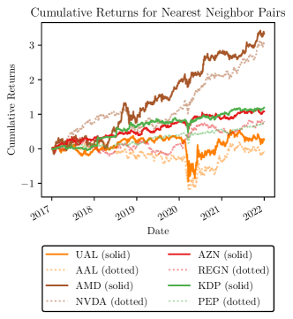
Figure 3: Cummulative Returns for assets with the closest Energy Distances.

Figure 3 illustrates the cumulative returns over time for nearest neighbor pairs, with solid and dotted lines representing each firm in a pair. Strong correlation in returns is observed across all pairs, suggesting that the Energy Distance metric successfully identifies firms with similar return trajectories.

For example, United Airlines (UAL) and American Airlines (AAL) show highly correlated movements, particularly reflecting the volatility experienced during the COVID-19 pandemic. Similarly, AMD (Advanced Micro Devices Inc) and NVIDIA (NVDA) exhibit closely aligned performance trends, likely driven by their shared presence in the semiconductor industry.

Overall, this visualization highlights the high degree of correlation within each pair, affirming that the Energy Distance metric captures meaningful relationships in terms of return behavior.

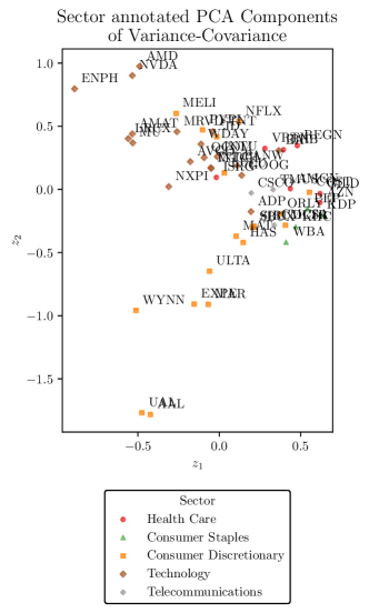
Figure 4: PCA projection of firms variance-covariance matrix annotated by ticker and coloured by sector. To aid in visual analysis, the components have undergone an linear transformation to minimize the L2 distance between the PCA projection of tickers and those presented in Figure 2.

In Figure 4, we show a biplot of the PCA projection of the firms’ variance-covariance matrix. In this plot, the firms are colored by their respective sectors, and the points are annotated with their tickers. To quantitatively assess the clustering tendency, we computed the Silhouette scores for the sector-level clusters based on the projected coordinates (Rousseeuw,, 1987)

The Silhouette score is a widely used metric to assess the quality of clustering by quantifying how well each data point lies within its cluster compared to other clusters. It provides a measure of how similar a point is to its own cluster (cohesion) relative to the closest neighboring cluster (separation). A high Silhouette score indicates that the data points are well-clustered, while a low or negative score suggests that the points may be assigned to the wrong cluster or are located between clusters.

For each data point $i$, the Silhouette score $s(i)$ is computed as follows. First, the cohesion, denoted as $a(i)$, is calculated as the average distance between the point $i$ and all other points within the same cluster $C_{I}$:

$$a(i)=\frac{1}{|C_{I}|-1}\sum_{j\in C_{I},i\neq j}d(i,j)$$

where $d(i,j)$ represents the distance between points $i$ and $j$, and $|C_{I}|$ is the number of points in cluster $C_{I}$. This measures how well the point $i$ is assigned to its own cluster. The separation, denoted as $b(i)$, is the minimum average distance between the point $i$ and all points in any other cluster $C_{J}$ (where $C_{J}\neq C_{I}$):

$$b(i)=\min_{J\neq I}\frac{1}{|C_{J}|}\sum_{j\in C_{J}}d(i,j)$$

This measures the dissimilarity between the point $i$ and its neighboring clusters. The Silhouette score $s(i)$ is then defined as:

$$s(i)=\frac{b(i)-a(i)}{\max\{a(i),b(i)\}}$$

If $E[s(i)]$ is close to 0, it suggests that, on average, firms from different sectors are not well-separated and may lie near the boundaries between sectors. A negative value of $E[s(i)]$ would indicate that, on average, firms are more similar to those in neighboring sectors, suggesting overlap or misclassification between sectors based on their projected positions.

Method	Silhouette Score
Energy Distance (original space)	0.085
Metric-MDS	0.057
PCA	-0.023

Table I: Silhouette scores for asset Sectors using different methods.

In Table I, the Silhouette score computed directly from the Energy Distance matrix is $0.085$, indicating a moderate level of clustering by sector. The Metric-MDS projection yields a slightly lower Silhouette score of $0.057$, while the PCA projection results in a negative score of $-0.023$, suggesting poor clustering of Sectors in the space.

These results suggest that the Energy Distance metric effectively captures sectoral similarities between firms based on the semantic content of news articles. The moderate Silhouette scores imply that firms within the same sector tend to have more similar distributions in the latent risk factor space $\Omega$, as reflected by their news embeddings. The fact that Metric-MDS preserves some of this clustering in two dimensions further supports the notion that the Energy Distance is aligned with sectoral classifications.

III-D Interpretation and Implications

The findings from our post-hoc analysis provide valuable insights into the nature of the Energy Distance metric in the context of financial assets. The clustering of firms by sector suggests that the Energy Distance, computed from the semantic content of news articles, captures meaningful economic relationships between assets. Specifically, firms operating within the same sector are likely influenced by similar industry-specific risk factors, which are reflected in the news coverage and, consequently, in their embeddings.

This observation reinforces the validity of using news embeddings as proxies for the latent sensitivity functions $\beta_{i}(\omega)$. By capturing sectoral and thematic information, the embeddings help approximate the distribution of assets in the continuous risk factor space $\Omega$. The alignment between the Energy Distance and sector classifications implies that our approach effectively identifies common risk factors that drive asset returns.

From a financial perspective, these insights have significant implications for risk management and portfolio construction. Understanding the latent relationships between assets based on semantic analysis allows investors to identify hidden correlations that may not be apparent from historical return data alone. This can enhance portfolio diversification by avoiding unintended concentrations in certain risk factors. Additionally, incorporating such latent information can improve the accuracy of risk forecasts and stress testing, leading to more robust investment strategies.

III-E Applications in Financial Risk Management

While traditional asset pricing models rely heavily on market data to estimate covariance and correlations, the continuous risk factor model proposed in this paper offers a distinct advantage: it does not depend on observable asset prices. Instead, by leveraging latent risk factor distributions, this approach opens the door to a broader set of applications, particularly in scenarios where market data is incomplete, unreliable, or altogether absent.

This is particularly relevant in cases where assets are newly listed or where historical price data is sparse, such as with recent IPOs or newly established markets. Moreover, the model’s potential extends to assets that have been de-listed, thinly traded, or illiquid, situations where price volatility or the lack of trading activity makes traditional risk estimation methods unreliable. For example, private equity investments, where market prices are often unavailable, can benefit from this model’s capacity to infer risk factors based on non-price-based data.

Further, sovereign wealth funds and large institutional investors, which frequently hold stakes in illiquid assets such as infrastructure projects or private ventures, face challenges in pricing these investments for risk management purposes. In these cases, traditional models that rely on active market data often fall short. By contrast, the continuous risk factor model, supported by textual data such as news content or fundamental analysis, provides a promising alternative for estimating the covariance structure without requiring frequent price updates. This could also prove valuable in emerging markets or in situations where trading has been temporarily suspended due to regulatory issues, natural disasters, or market crises.

Such applications suggest that the method is not only theoretically robust but also practically versatile. By offering a tool that circumvents the need for price-based data, the model holds potential for investors and fund managers in circumstances where market data is either unreliable or non-existent. This flexibility makes it a valuable addition to the existing toolkit for portfolio diversification and risk management, particularly for institutional investors managing complex portfolios with illiquid or non-traditional assets.

IV Conclusion

In this study, we introduced a novel approach to modelling the relationships between asset returns and their underlying risk factors using the framework of Energy Distance and advanced natural language processing techniques. By leveraging semantic embeddings derived from news articles, we approximated the latent sensitivity functions $\beta_{i}(\omega)$ for each asset and computed the Energy Distances between them.

Our empirical results demonstrate a significant correlation between the Energy Distance and the observed return correlations of assets, as confirmed by Mantel’s test. This indicates that the Energy Distance provides an upper bound on asset correlations, aligning with theoretical expectations. The post-hoc analysis further revealed that the Energy Distance captures sectoral similarities among firms, suggesting that our method effectively identifies common risk factors embedded in the semantic content of news.

These findings have important implications for financial risk management and portfolio construction. By incorporating semantic information from textual data, investors can gain deeper insights into the latent risk factors driving asset returns. This approach enhances the understanding of the covariance structure between assets, potentially leading to improved diversification strategies and more accurate risk assessments.

The continuous risk factor model outlined in this paper offers significant potential for financial risk management, particularly in situations where market data is unreliable or unavailable. This includes newly listed assets, illiquid or thinly traded securities, private equity investments, and assets managed by institutional investors such as sovereign wealth funds. By bypassing the need for direct price observation and leveraging latent risk factors, this method provides a versatile alternative to traditional risk models, offering a robust framework for managing portfolios in a broader range of financial contexts.

Appendix .A Variance of an Assetś Returns

Using the result from Section II-A, the expression for the variance of $\tilde{R_{i,t}}$ can now be derived as follows. Recall that the return of asset $i$ is given by:

$$\tilde{R_{i,t}}=\int_{\Omega}\beta_{i}(\omega)\lambda_{t}(\omega)d\omega,$$ (63)

where $\beta_{i}(\omega)$ represents the factor loading for asset $i$ and $\lambda_{t}(\omega)$ is the factor realization at time $t$. To compute the variance of $\tilde{R_{i,t}}$, we apply the definition of variance:

$$\operatorname{Var}(\tilde{R_{i,t}})=E[\tilde{R_{i,t}}^{2}]-(E[\tilde{R_{i,t}}])^{2}.$$ (64)

First, we need to evaluate $E[\tilde{R_{i,t}}^{2}]$, which involves squaring the return expression. Squaring $\tilde{R_{i,t}}$ yields a double integral:

$$\tilde{R_{i,t}}^{2}=\left(\int_{\Omega}\beta_{i}(\omega)\lambda_{t}(\omega)d\omega\right)^{2}=\int_{\Omega}\int_{\Omega}\beta_{i}(\omega)\beta_{i}(\omega^{\prime})\lambda_{t}(\omega)\lambda_{t}(\omega^{\prime})d\omega d\omega^{\prime}.$$ (65)

Taking the expectation of this expression gives:

$$E[\tilde{R_{i,t}}^{2}]=\int_{\Omega}\int_{\Omega}\beta_{i}(\omega)\beta_{i}(\omega^{\prime})E[\lambda_{t}(\omega)\lambda_{t}(\omega^{\prime})]d\omega d\omega^{\prime}.$$ (66)

Using the identity for the expectation of the product of random variables:

$$E[\lambda_{t}(\omega)\lambda_{t}(\omega^{\prime})]=\operatorname{Cov}(\lambda_{t}(\omega),\lambda_{t}(\omega^{\prime}))+E[\lambda_{t}(\omega)]E[\lambda_{t}(\omega^{\prime})],$$ (67)

we can split the expectation into two terms. Under the assumption that $\lambda_{t}(\omega)$ and $\lambda_{t}(\omega^{\prime})$ are uncorrelated across different states $\omega\neq\omega^{\prime}$, as in the case of the dirac delta function or constant covariance function, the covariance term vanishes. This simplifies the expectation for $\omega=\omega^{\prime}$ to:

$$E[\lambda_{t}^{2}(\omega)]=\operatorname{Var}[\lambda_{t}(\omega)]+\left(E[\lambda_{t}(\omega)]\right)^{2}.$$ (68)

Thus, the expectation $E[\tilde{R_{i,t}}^{2}]$ simplifies to:

$$E[\tilde{R_{i,t}}^{2}]=\int_{\Omega}\beta_{i}^{2}(\omega)\left(\operatorname{Var}[\lambda_{t}(\omega)]+\left(E[\lambda_{t}(\omega)]\right)^{2}\right)d\omega.$$ (69)

Next, we subtract $(E[\tilde{R_{i,t}}])^{2}$, where $E[\tilde{R_{i,t}}]$ is given by:

$$E[\tilde{R_{i,t}}]=\int_{\Omega}\beta_{i}(\omega)E[\lambda_{t}(\omega)]d\omega.$$ (70)

Squaring this yields:

$$(E[\tilde{R_{i,t}}])^{2}=\left(\int_{\Omega}\beta_{i}(\omega)E[\lambda_{t}(\omega)]d\omega\right)^{2}.$$ (71)

Finally, subtracting this from $E[\tilde{R_{i,t}}^{2}]$ cancels out the terms involving $\left(E[\lambda_{t}(\omega)]\right)^{2}$, leaving:

$$\operatorname{Var}(\tilde{R_{i,t}})=\int_{\Omega}\beta_{i}^{2}(\omega)\operatorname{Var}[\lambda_{t}(\omega)]d\omega.$$ (72)

This result shows that the variance of the return $\tilde{R_{i,t}}$ is a weighted sum of the variances of the factor realizations $\lambda_{t}(\omega)$, with the weights given by the square of the factor loadings $\beta_{i}(\omega)$.

Appendix .B Dictionary of Nasdaq Symbols

Symbol	Company Name	Sector
BIIB	Biogen Inc. Common Stock	Health Care
WBA	Walgreens Boots Alliance, Inc. Common Stock	Consumer Staples
HAS	Hasbro, Inc. Common Stock	Consumer Discretionary
NXPI	NXP Semiconductors N.V. Common Stock	Technology
NVDA	NVIDIA Corporation Common Stock	Technology
DLTR	Dollar Tree Inc. Common Stock	Consumer Discretionary
AMD	Advanced Micro Devices, Inc. Common Stock	Technology
ISRG	Intuitive Surgical, Inc. Common Stock	Health Care
AZN	AstraZeneca PLC American Depositary Shares	Health Care
JD	JD.com, Inc. American Depositary Shares	Consumer Discretionary
EA	Electronic Arts Inc. Common Stock	Technology
MTCH	Match Group, Inc. Common Stock	Technology
ALGN	Align Technology, Inc. Common Stock	Health Care
AVGO	Broadcom Inc. Common Stock	Technology
ORLY	O’Reilly Automotive, Inc. Common Stock	Consumer Discretionary
ENPH	Enphase Energy, Inc. Common Stock	Technology
LRCX	Lam Research Corporation Common Stock	Technology
KHC	The Kraft Heinz Company Common Stock	Consumer Staples
SIRI	SiriusXM Holdings Inc. Common Stock	Consumer Discretionary
WDAY	Workday, Inc. Class A Common Stock	Technology
MRVL	Marvell Technology, Inc. Common Stock	Technology
AMGN	Amgen Inc. Common Stock	Health Care
MAT	Mattel, Inc. Common Stock	Consumer Discretionary
TMUS	T-Mobile US, Inc. Common Stock	Telecommunications
WYNN	Wynn Resorts, Limited Common stock	Consumer Discretionary
INTC	Intel Corporation Common Stock	Technology
GOOG	Alphabet Inc. Class C Capital Stock	Technology
ULTA	Ulta Beauty, Inc. Common Stock	Consumer Discretionary
GILD	Gilead Sciences, Inc. Common Stock	Health Care
CSCO	Cisco Systems, Inc. Common Stock (DE)	Telecommunications
AMAT	Applied Materials, Inc. Common Stock	Technology
PYPL	PayPal Holdings, Inc. Common Stock	Consumer Discretionary
ZS	Zscaler, Inc. Common Stock	Technology
FTNT	Fortinet, Inc. Common Stock	Technology
LULU	lululemon athletica inc. Common Stock	Consumer Discretionary
QCOM	QUALCOMM Incorporated Common Stock	Technology
PEP	PepsiCo, Inc. Common Stock	Consumer Staples
SBUX	Starbucks Corporation Common Stock	Consumer Discretionary
AAL	American Airlines Group Inc. Common Stock	Consumer Discretionary
REGN	Regeneron Pharmaceuticals, Inc. Common Stock	Health Care
INTU	Intuit Inc. Common Stock	Technology
UAL	United Airlines Holdings, Inc. Common Stock	Consumer Discretionary
COST	Costco Wholesale Corporation Common Stock	Consumer Discretionary
KDP	Keurig Dr Pepper Inc. Common Stock	Consumer Staples
CMCSA	Comcast Corporation Class A Common Stock	Telecommunications
ADP	Automatic Data Processing, Inc. Common Stock	Technology
NFLX	Netflix, Inc. Common Stock	Consumer Discretionary
MELI	MercadoLibre, Inc. Common Stock	Consumer Discretionary
MU	Micron Technology, Inc. Common Stock	Technology
VRTX	Vertex Pharmaceuticals Incorporated Common Stock	Health Care
MAR	Marriott International Class A Common Stock	Consumer Discretionary
EXPE	Expedia Group, Inc. Common Stock	Consumer Discretionary
PANW	Palo Alto Networks, Inc. Common Stock	Technology

References

- Araci, (2019) Araci, D. (2019). FinBERT: Financial Sentiment Analysis with Pre-trained Language Models.
- Bera et al., (2016) Bera, A. K., Sebnem, E., and Kececi, N. F. (2016). Spatial Dependence in Financial Data: Importance of the Weights Matrix. Arthaniti-Journal of Economic Theory and Practice, 15(2):29–42.
- Bordea et al., (2016) Bordea, G., Lefever, E., and Buitelaar, P. (2016). SemEval-2016 Task 13: Taxonomy Extraction Evaluation (TExEval-2). pages 1081–1091.
- CFA Institute, (2017) CFA Institute (2017). CFA Program Curriculum 2018 Level II. John Wiley & Sons.
- Chopra and Ghosh, (2021) Chopra, A. and Ghosh, S. (2021). Term Expansion and FinBERT fine-tuning for Hypernym and Synonym Ranking of Financial Terms.
- Daniel and Titman, (1997) Daniel, K. and Titman, S. (1997). Evidence on the characteristics of cross sectional variation in stock returns. The Journal of Finance, 52(1):1–33.
- Dao et al., (2022) Dao, T., Fu, D. Y., Ermon, S., Rudra, A., and Ré, C. (2022). FlashAttention: Fast and Memory-Efficient Exact Attention with IO-Awareness. volume 35, pages 16344–16359.
- Desola et al., (2019) Desola, V., Hanna, K., and Nonis, P. (2019). FinBERT: pre-trained model on SEC filings for financial natural language tasks.
- Devlin et al., (2019) Devlin, J., Chang, M.-W., Lee, K., and Toutanova, K. (2019). BERT: Pre-training of Deep Bidirectional Transformers for Language Understanding. arXiv:1810.04805 [cs].
- Fama and French, (1996) Fama, E. F. and French, K. R. (1996). Multifactor Explanations of Asset Pricing Anomalies. The Journal of Finance, 51(1):55–84.
- Fernandez, (2011) Fernandez, V. (2011). Spatial linkages in international financial markets. Quantitative Finance, 11(2):237–245.
- Garcıa, (2013) Garcıa, D. (2013). Sentiment during recessions. The Journal of Finance, 68(3):1267–1300.
- Ge et al., (2023) Ge, S., Li, S., and Linton, O. (2023). News-Implied Linkages and Local Dependency in the Equity Market. Journal of Econometrics, 235(2):779–815.
- Isma¨ıl et al., (2020) Isma¨ıl, I., Maarouf, E., Mansar, Y., Mouilleron, V., and Valsamou-Stanislawski, D. (2020). The FinSim 2020 Shared Task: Learning Semantic Representations for the Financial Domain.
- Kang et al., (2021) Kang, J., Bellato, S., Gan, M., and Maarouf, I. E. (2021). FinSim-3: The 3rd Shared Task on Learning Semantic Similarities for the Financial Domain.
- Kou et al., (2018) Kou, S., Peng, X., and Zhong, H. (2018). Asset Pricing with Spatial Interaction. Management Science, 64(5):2083–2101.
- Kruskal, (1964) Kruskal, J. B. (1964). Multidimensional scaling by optimizing goodness of fit to a nonmetric hypothesis. Psychometrika, 29(1):1–27.
- Mansar et al., (2021) Mansar, Y., Kang, J., and Maarouf, I. E. (2021). The finsim-2 2021 shared task: Learning semantic similarities for the financial domain. In Companion Proceedings of the Web Conference 2021, pages 288–292.
- Mantel, (1967) Mantel, N. (1967). The detection of disease clustering and a generalized regression approach. Cancer research, Cancer research(2):209–220.
- Menzly and Ozbas, (2010) Menzly, L. and Ozbas, O. (2010). Market Segmentation and Cross-predictability of Returns. The Journal of Finance, 65(4):1555–1580.
- Neto, (2024) Neto, E. C. (2024). Computationally efficient permutation tests for the multivariate two-sample problem based on energy distance or maximum mean discrepancy statistics. arXiv:2406.06488 [stat].
- Nussbaum et al., (2024) Nussbaum, Z., Morris, J. X., Duderstadt, B., and Mulyar, A. (2024). Nomic Embed: Training a Reproducible Long Context Text Embedder.
- Pei and Zhang, (2021) Pei, Y. and Zhang, Q. (2021). GOAT at the FinSim-2 task: Learning Word Representations of Financial Data with Customized Corpus. In The Web Conference 2021 - Companion of the World Wide Web Conference, WWW 2021, pages 307–310. Association for Computing Machinery, Inc.
- Peng et al., (2021) Peng, B., Chersoni, E., Hsu, Y.-Y., and Huang, C.-R. (2021). Is Domain Adaptation Worth Your Investment? Comparing BERT and FinBERT on Financial Tasks. Punta Cana and online, pages 37–44.
- Radford et al., (2017) Radford, A., Jozefowicz, R., and Sutskever, I. (2017). Learning to Generate Reviews and Discovering Sentiment. arXiv:1704.01444 [cs].
- Ross, (1976) Ross, S. (1976). The arbitrage pricing theory. Journal of Economic Theory, 13(3):341–360.
- Rousseeuw, (1987) Rousseeuw, P. J. (1987). Silhouettes: A graphical aid to the interpretation and validation of cluster analysis. Journal of Computational and Applied Mathematics, 20:53–65.
- Scherbina and Schlusche, (2013) Scherbina, A. and Schlusche, B. (2013). Economic Linkages Inferred from News Stories and the Predictability of Stock Returns. SSRN Electronic Journal.
- Schwenkler and Zheng, (2020) Schwenkler, G. and Zheng, H. (2020). The network of firms implied by the news.
- Su et al., (2023) Su, J., Lu, Y., Pan, S., Murtadha, A., Wen, B., and Liu, Y. (2023). RoFormer: Enhanced Transformer with Rotary Position Embedding. arXiv:2104.09864 [cs].
- Tetlock, (2007) Tetlock, P. C. (2007). Giving Content to Investor Sentiment: The Role of Media in the Stock Market. The Journal of Finance, 62(3):1139–1168.
Appendix \thechapter.A Variance of an Assetś Returns