COMAL: A Convergent Meta-Algorithm for Aligning LLMs with General Preferences

Abstract

Many alignment methods, including reinforcement learning from human feedback (RLHF), rely on the Bradley-Terry reward assumption, which is insufficient to capture the full range of general human preferences. To achieve robust alignment with general preferences, we model the alignment problem as a two-player zero-sum game, where the Nash equilibrium policy guarantees a 50% win rate against any competing policy. However, previous algorithms for finding the Nash policy either diverge or converge to a Nash policy in a modified game, even in a simple synthetic setting, thereby failing to maintain the 50% win rate guarantee against all other policies. We propose a meta-algorithm, Convergent Meta Alignment Algorithm (COMAL), for language model alignment with general preferences, inspired by convergent algorithms in game theory. Theoretically, we prove that our meta-algorithm converges to an exact Nash policy in the last iterate. Additionally, our meta-algorithm is simple and can be integrated with many existing methods designed for RLHF and preference optimization with minimal changes. Experimental results demonstrate the effectiveness of the proposed framework when combined with existing preference policy optimization methods.

1 Introduction

Large Language Models (LLMs) (Brown et al., 2020; OpenAI, 2023; Dubey et al., 2024) have fundamentally transformed the fields of natural language processing and artificial intelligence. They excel in tasks ranging from text generation and translation to complex question answering and interactive dialogue systems. As these models become more integrated into daily life, a key challenge is ensuring they achieve high levels of alignment with human values and preferences.

One of the most widely adopted approaches to addressing this challenge is Reinforcement Learning from Human Feedback (RLHF) (Christiano et al., 2017; Ouyang et al., 2022). This framework consists of two steps: first, learning a reward model from a dataset containing human preferences, and second, optimizing the LLM using the proximal policy optimization (PPO) algorithm (Schulman et al., 2017). Recently,  Rafailov et al. (2024) observed that the first step can be bypassed, proposing the direct preference optimization (DPO) algorithm, directly optimizing the LLM from the dataset.

However, the aforementioned approaches crucially rely on the assumption that human preferences can be expressed using the Bradley-Terry (BT) model (Bradley and Terry, 1952). Unfortunately, the BT model is too restrictive to capture the richness and complexity of human preferences. Specifically, the BT model can only induce transitive preferences – i.e., if more people favor A over B, and B over C, then more people must favor A over C. Such transitivity may not hold in the presence of diverse populations and is also incompatible with evidence from human decision-making (May, 1954; Tversky, 1969).

To overcome this limitation, recent research has begun to explore alignment under general preferences.  Munos et al. (2024) formulate this alignment problem as a symmetric two-player zero-sum game, where both players’ strategies are LLMs, and their payoffs are determined by the win rate against the opponent’s LLM according to the preference model. The objective is to identify a Nash equilibrium policy that guarantees at least a 50% win rate against any other policy (Munos et al., 2024; Swamy et al., 2024; Azar et al., 2024; Calandriello et al., 2024), a property we refer to as robust alignment. However, all the proposed algorithms either diverge or converge to the Nash policy of a modified game, thereby failing to maintain the 50% win rate guarantee against all other policies.

Our Contribution.

We introduce a novel meta-algorithm, Convergent Meta Alignment Algorithm (COMAL), inspired by the conceptual prox-method, a convergent algorithm for solving two-player zero-sum games (Nemirovski, 2004). Our first observation is that many existing algorithms, including PPO (Schulman et al., 2017), DPO (Rafailov et al., 2024), IPO (Azar et al., 2024), SPPO (Wu et al., 2024), REBEL (Gao et al., 2024), DRO (Richemond et al., 2024), INPO (Zhang et al., 2024), etc., can be interpreted as implementations of the $\operatorname{Prox}$ operator (Nemirovski, 2004). COMAL employs the $\operatorname{Prox}$ operator as its fundamental building block and provably converges to the Nash equilibrium policy in the last iterate, assuming the $\operatorname{Prox}$ operator can be computed exactly, thus achieving robust alignment. This approach allows us to leverage many existing algorithms in a black-box manner. While several algorithms, e.g., IPO, SPPO, etc., in the literature demonstrate average-iterate convergence to the Nash equilibrium policy, they all diverge in the last iterate. Unfortunately, iterate averaging can be cumbersome, particularly when deep-learning components are involved, as it may not be feasible to average the outputs of LLMs. For the more desirable last-iterate convergence (Munos et al., 2024; Zhang et al., 2024), existing algorithms only guarantee convergence to a KL-regularized Nash equilibrium, which does not have the robust alignment property. Compared to these algorithms, COMAL is the first to provably converge to a Nash equilibrium policy in the last iterate, thus guaranteeing robust alignment.

In addition to our theoretical analysis, we validate the effectiveness of COMAL through both synthetic and LLM-based experiments.

Synthetic experiments.

We construct a $3\times 3$ two-player zero-sum preference game and compare COMAL with a wide range of algorithms proposed in the literature. The result clearly shows that COMAL is the only algorithm that converges to the Nash equilibrium of the game in the last iterate.

LLM-based experiments.

Furthermore, we evaluate the performance of COMAL against existing preference optimization algorithms under a practical setting, where a pre-trained LLM, Qwen2-1.5B (Yang et al., 2024) is fine-tuned using different algorithms on the UltraFeedback (Cui et al., 2023) dataset, which is commonly used for alignment fine-tuning of LLMs. We run iterative algorithms up to 42 iterations and compare both the best and the last checkpoints. Our experimental results demonstrate the advantages of COMAL: it consistently achieves a win rate strictly above 50% compared to baseline algorithms, including DPO (Rafailov et al., 2024) and iterative algorithms such as iterative IPO (Azar et al., 2024) and INPO (Zhang et al., 2024).

2 Background

We use $\Delta(\mathcal{Z})$ to denote a distribution over a set $\mathcal{Z}$. We denote $x\in\mathcal{X}$ as an instruction where $\mathcal{X}$ is the instruction set. We assume a fixed distribution $\rho\in\Delta(\mathcal{X})$ over the instruction set. We denote $\mathcal{Y}$ as the response set and $y\in\mathcal{Y}$ as one response. Given any instruction $x\in\mathcal{X}$, an LLM policy $\pi$ specifies the output distribution $\pi(\cdot\mid x)\in\Delta(\mathcal{Y})$. For distributions $p,q\in\Delta(\mathcal{Z})$, the Kullback-Leibler (KL) divergence is defined as $\operatorname{KL}(p||q):=\sum_{z\in\mathcal{Z}}p(z)\log\frac{p(z)}{q(z)}$. The sigmoid function is $\sigma(x):=\frac{e^{x}}{e^{x}+1}$. We use $\mathrm{supp}(p)$ to denote the support of a distribution $p$.

Preference Models

In this paper, we focus on general preference models.

Definition 1 (General Preference Model).

A general preference model $\mathbb{P}:\mathcal{X}\times\mathcal{Y}\times\mathcal{Y}\rightarrow[0,1]$ satisfies $\mathbb{P}(y_{1}\succ y_{2}\mid x)=1-\mathbb{P}(y_{2}\succ y_{1}\mid x)$. When we query $\mathbb{P}$ with $(x,y_{1},y_{2})$, it outputs $1$ with probability $\mathbb{P}(y_{1}\succ y_{2}\mid x)$ meaning $y_{1}$ is preferred over $y_{2}$, and it outputs $0$ otherwise.

We define $\mathbb{P}(\pi_{1}\succ\pi_{2}):=\mathbb{E}_{x\sim\rho}{\mathchoice{\left[\mathbb{E}_{y_{1}\sim\pi_{1},y_{2}\sim\pi_{2}}{\mathchoice{\left[\mathbb{P}(y_{1}\succ y_{2}\mid x)\right]}{[\mathbb{P}(y_{1}\succ y_{2}\mid x)]}{[\mathbb{P}(y_{1}\succ y_{2}\mid x)]}{[\mathbb{P}(y_{1}\succ y_{2}\mid x)]}}\right]}{[\mathbb{E}_{y_{1}\sim\pi_{1},y_{2}\sim\pi_{2}}{\mathchoice{\left[\mathbb{P}(y_{1}\succ y_{2}\mid x)\right]}{[\mathbb{P}(y_{1}\succ y_{2}\mid x)]}{[\mathbb{P}(y_{1}\succ y_{2}\mid x)]}{[\mathbb{P}(y_{1}\succ y_{2}\mid x)]}}]}{[\mathbb{E}_{y_{1}\sim\pi_{1},y_{2}\sim\pi_{2}}{\mathchoice{\left[\mathbb{P}(y_{1}\succ y_{2}\mid x)\right]}{[\mathbb{P}(y_{1}\succ y_{2}\mid x)]}{[\mathbb{P}(y_{1}\succ y_{2}\mid x)]}{[\mathbb{P}(y_{1}\succ y_{2}\mid x)]}}]}{[\mathbb{E}_{y_{1}\sim\pi_{1},y_{2}\sim\pi_{2}}{\mathchoice{\left[\mathbb{P}(y_{1}\succ y_{2}\mid x)\right]}{[\mathbb{P}(y_{1}\succ y_{2}\mid x)]}{[\mathbb{P}(y_{1}\succ y_{2}\mid x)]}{[\mathbb{P}(y_{1}\succ y_{2}\mid x)]}}]}}$ as the win rate of $\pi_{1}$ over $\pi_{2}$ under preference model $\mathbb{P}$. We denote the preference distribution $\lambda_{\mathbb{P}}(y,y^{\prime})$ as a binary distribution:

$$\lambda_{\mathbb{P}}(y,y^{\prime})=\begin{cases}(y,y^{\prime})\text{ with probability $\mathbb{P}[y\succ y^{\prime}]$}\\ (y^{\prime},y)\text{ with probability $1-\mathbb{P}[y\succ y^{\prime}]$}\\ \end{cases}$$ (1)

A special case of the general preference model is the Bradley-Terry (BT) model, which assumes a reward function parameterizes the preference.

Definition 2 (Bradley-Terry Model).

A preference model $\mathbb{P}$ satisfies the Bradley-Terry (BT) assumption if there exists a reward function $r^{*}:\mathcal{X}\times\mathcal{Y}\rightarrow\mathbb{R}$ such that

$$\mathbb{P}(y_{1}\succ y_{2}\mid x)=\frac{\exp{\mathchoice{\left(r^{*}(x,y_{1})\right)}{(r^{*}(x,y_{1}))}{(r^{*}(x,y_{1}))}{(r^{*}(x,y_{1}))}}}{\exp{\mathchoice{\left(r^{*}(x,y_{1})\right)}{(r^{*}(x,y_{1}))}{(r^{*}(x,y_{1}))}{(r^{*}(x,y_{1}))}}+\exp{\mathchoice{\left(r^{*}(x,y_{2})\right)}{(r^{*}(x,y_{2}))}{(r^{*}(x,y_{2}))}{(r^{*}(x,y_{2}))}}}=\sigma(r^{*}(x,y_{1})-r^{*}(x,y_{2})).$$

2.1 Alignment under the Bradley-Terry Model Assumption

RLHF

The canonical formulation of Reinforcement Learning from Human Feedback (RLHF) is to first learn a reward function $r$ under the BT model and then find the optimal KL regularized policy $\pi^{*}$ with respect to the learned reward function $r$:

$$\pi^{*}:=\arg\max_{\pi}\mathbb{E}_{x\sim\rho,y\sim\pi(\cdot\mid x)}{\mathchoice{\left[r(x,y)-\eta^{-1}\operatorname{KL}(\pi(\cdot\mid x)||\pi_{\mathrm{ref}}(\cdot\mid x))\right]}{[r(x,y)-\eta^{-1}\operatorname{KL}(\pi(\cdot\mid x)||\pi_{\mathrm{ref}}(\cdot\mid x))]}{[r(x,y)-\eta^{-1}\operatorname{KL}(\pi(\cdot\mid x)||\pi_{\mathrm{ref}}(\cdot\mid x))]}{[r(x,y)-\eta^{-1}\operatorname{KL}(\pi(\cdot\mid x)||\pi_{\mathrm{ref}}(\cdot\mid x))]}},$$ (2)

where $\eta^{-1}>0$ controls the regularization, and $\pi_{\mathrm{ref}}$ is the initial reference model, usually the policy $\pi_{\mathrm{sft}}$ obtained from pre-training and supervised fine-tuning.

DPO

Rafailov et al. (2024) observe that the regularized optimization problem (2) has a closed-form solution: for any $x$ and $y$,

$$\pi^{*}(y\mid x)=\frac{\pi_{\mathrm{ref}}(y\mid x)\exp{\mathchoice{\left(\eta r(x,y)\right)}{(\eta r(x,y))}{(\eta r(x,y))}{(\eta r(x,y))}}}{Z_{x}},$$ (3)

where $Z_{x}=\mathbb{E}_{y\sim\pi_{\mathrm{ref}}(\cdot\mid x)}{\mathchoice{\left[\exp(\frac{1}{\eta}r(y,x))\right]}{[\exp(\frac{1}{\eta}r(y,x))]}{[\exp(\frac{1}{\eta}r(y,x))]}{[\exp(\frac{1}{\eta}r(y,x))]}}$ is the normalization constant known as the partition function. In (3), we see that $\pi^{*}$ implicitly parameterizes the reward function $r$. Rafailov et al. (2024) propose direct preference optimization (DPO) to learn the optimal policy using the maximum likelihood objective directly:

$$\ell_{\mathrm{DPO}}(\pi;\pi_{\mathrm{ref}})=-\mathbb{E}_{(x,y_{w},y_{l})\sim\mathcal{D}}{\mathchoice{\left[\log\sigma{\mathchoice{\left(\eta^{-1}\log\frac{\pi(y_{w}\mid x)}{\pi_{\mathrm{ref}}(y_{w}\mid x)}-\eta^{-1}\log\frac{\pi(y_{l}\mid x)}{\pi_{\mathrm{ref}}(y_{l}\mid x)}\right)}{(\eta^{-1}\log\frac{\pi(y_{w}\mid x)}{\pi_{\mathrm{ref}}(y_{w}\mid x)}-\eta^{-1}\log\frac{\pi(y_{l}\mid x)}{\pi_{\mathrm{ref}}(y_{l}\mid x)})}{(\eta^{-1}\log\frac{\pi(y_{w}\mid x)}{\pi_{\mathrm{ref}}(y_{w}\mid x)}-\eta^{-1}\log\frac{\pi(y_{l}\mid x)}{\pi_{\mathrm{ref}}(y_{l}\mid x)})}{(\eta^{-1}\log\frac{\pi(y_{w}\mid x)}{\pi_{\mathrm{ref}}(y_{w}\mid x)}-\eta^{-1}\log\frac{\pi(y_{l}\mid x)}{\pi_{\mathrm{ref}}(y_{l}\mid x)})}}\right]}{[\log\sigma{\mathchoice{\left(\eta^{-1}\log\frac{\pi(y_{w}\mid x)}{\pi_{\mathrm{ref}}(y_{w}\mid x)}-\eta^{-1}\log\frac{\pi(y_{l}\mid x)}{\pi_{\mathrm{ref}}(y_{l}\mid x)}\right)}{(\eta^{-1}\log\frac{\pi(y_{w}\mid x)}{\pi_{\mathrm{ref}}(y_{w}\mid x)}-\eta^{-1}\log\frac{\pi(y_{l}\mid x)}{\pi_{\mathrm{ref}}(y_{l}\mid x)})}{(\eta^{-1}\log\frac{\pi(y_{w}\mid x)}{\pi_{\mathrm{ref}}(y_{w}\mid x)}-\eta^{-1}\log\frac{\pi(y_{l}\mid x)}{\pi_{\mathrm{ref}}(y_{l}\mid x)})}{(\eta^{-1}\log\frac{\pi(y_{w}\mid x)}{\pi_{\mathrm{ref}}(y_{w}\mid x)}-\eta^{-1}\log\frac{\pi(y_{l}\mid x)}{\pi_{\mathrm{ref}}(y_{l}\mid x)})}}]}{[\log\sigma{\mathchoice{\left(\eta^{-1}\log\frac{\pi(y_{w}\mid x)}{\pi_{\mathrm{ref}}(y_{w}\mid x)}-\eta^{-1}\log\frac{\pi(y_{l}\mid x)}{\pi_{\mathrm{ref}}(y_{l}\mid x)}\right)}{(\eta^{-1}\log\frac{\pi(y_{w}\mid x)}{\pi_{\mathrm{ref}}(y_{w}\mid x)}-\eta^{-1}\log\frac{\pi(y_{l}\mid x)}{\pi_{\mathrm{ref}}(y_{l}\mid x)})}{(\eta^{-1}\log\frac{\pi(y_{w}\mid x)}{\pi_{\mathrm{ref}}(y_{w}\mid x)}-\eta^{-1}\log\frac{\pi(y_{l}\mid x)}{\pi_{\mathrm{ref}}(y_{l}\mid x)})}{(\eta^{-1}\log\frac{\pi(y_{w}\mid x)}{\pi_{\mathrm{ref}}(y_{w}\mid x)}-\eta^{-1}\log\frac{\pi(y_{l}\mid x)}{\pi_{\mathrm{ref}}(y_{l}\mid x)})}}]}{[\log\sigma{\mathchoice{\left(\eta^{-1}\log\frac{\pi(y_{w}\mid x)}{\pi_{\mathrm{ref}}(y_{w}\mid x)}-\eta^{-1}\log\frac{\pi(y_{l}\mid x)}{\pi_{\mathrm{ref}}(y_{l}\mid x)}\right)}{(\eta^{-1}\log\frac{\pi(y_{w}\mid x)}{\pi_{\mathrm{ref}}(y_{w}\mid x)}-\eta^{-1}\log\frac{\pi(y_{l}\mid x)}{\pi_{\mathrm{ref}}(y_{l}\mid x)})}{(\eta^{-1}\log\frac{\pi(y_{w}\mid x)}{\pi_{\mathrm{ref}}(y_{w}\mid x)}-\eta^{-1}\log\frac{\pi(y_{l}\mid x)}{\pi_{\mathrm{ref}}(y_{l}\mid x)})}{(\eta^{-1}\log\frac{\pi(y_{w}\mid x)}{\pi_{\mathrm{ref}}(y_{w}\mid x)}-\eta^{-1}\log\frac{\pi(y_{l}\mid x)}{\pi_{\mathrm{ref}}(y_{l}\mid x)})}}]}},$$

where $\mathcal{D}$ is a data set containing win-loss pair of responses $\{y_{w},y_{l}\}$ given prompt $x$.

2.2 Robust Alignment with General Preference Models

The BT model assumption is insufficient to capture the full range of general human preferences (Munos et al., 2024; Swamy et al., 2024). To achieve robust alignment with general preferences, we model the policy optimization problem as a two-player zero-sum game with the objective function as follows:

$$J(\pi_{1},\pi_{2}):=\mathbb{P}(\pi_{1}\succ\pi_{2})-\frac{1}{2}=\mathbb{E}_{x\sim\rho}{\mathchoice{\left[\mathbb{E}_{y_{1}\sim\pi_{1},y_{2}\sim\pi_{2}}{\mathchoice{\left[\mathbb{P}(y_{1}\succ y_{2}\mid x)\right]}{[\mathbb{P}(y_{1}\succ y_{2}\mid x)]}{[\mathbb{P}(y_{1}\succ y_{2}\mid x)]}{[\mathbb{P}(y_{1}\succ y_{2}\mid x)]}}\right]}{[\mathbb{E}_{y_{1}\sim\pi_{1},y_{2}\sim\pi_{2}}{\mathchoice{\left[\mathbb{P}(y_{1}\succ y_{2}\mid x)\right]}{[\mathbb{P}(y_{1}\succ y_{2}\mid x)]}{[\mathbb{P}(y_{1}\succ y_{2}\mid x)]}{[\mathbb{P}(y_{1}\succ y_{2}\mid x)]}}]}{[\mathbb{E}_{y_{1}\sim\pi_{1},y_{2}\sim\pi_{2}}{\mathchoice{\left[\mathbb{P}(y_{1}\succ y_{2}\mid x)\right]}{[\mathbb{P}(y_{1}\succ y_{2}\mid x)]}{[\mathbb{P}(y_{1}\succ y_{2}\mid x)]}{[\mathbb{P}(y_{1}\succ y_{2}\mid x)]}}]}{[\mathbb{E}_{y_{1}\sim\pi_{1},y_{2}\sim\pi_{2}}{\mathchoice{\left[\mathbb{P}(y_{1}\succ y_{2}\mid x)\right]}{[\mathbb{P}(y_{1}\succ y_{2}\mid x)]}{[\mathbb{P}(y_{1}\succ y_{2}\mid x)]}{[\mathbb{P}(y_{1}\succ y_{2}\mid x)]}}]}}-\frac{1}{2}.$$ (4)

In this game, the max-player controls $\pi_{1}$ and tries to maximize $J(\pi_{1},\pi_{2})$ while the min-player controls $\pi_{2}$ and tries to minimize $J(\pi_{1},\pi_{2})$. We focus only on policies with $\Pi:=\{\pi:\mathrm{supp}(\pi)\subseteq\mathrm{supp}(\pi_{\mathrm{sft}})\}$ in the support of the initial SFT policy. A Nash equilibrium policy $(\pi_{1}^{\star},\pi_{2}^{\star})$ satisfies

$$\pi_{1}^{\star},\pi_{2}^{\star}\in\operatorname*{argmax}_{\pi_{1}\in\Pi}\operatorname*{argmin}_{\pi_{2}\in\Pi}J(\pi_{1},\pi_{2}),\quad J(\pi_{1},\pi_{2}^{\star})\leq J(\pi_{1}^{\star},\pi_{2}^{\star})\leq J(\pi_{1}^{\star},\pi_{2}),\forall\pi_{1},\pi_{2}\in\Pi.$$

Since $J(\pi_{1},\pi_{2})$ is symmetric, the game has a symmetric Nash equilibrium $(\pi^{\star},\pi^{\star})$. Moreover, the Nash equilibrium policy $\pi^{\star}$ guarantees that for any other policy $\pi$, its win rate is at least $\mathbb{P}(\pi^{\star}\succ\pi)\geq\mathbb{P}(\pi^{\star}\succ\pi^{\star})=50\%$. We call this property robust alignment. Our goal is to find a policy with robust alignment.

Existing online iterative preference optimization methods designed for or applicable to the original game, including iterative IPO (Azar et al., 2024) and SPPO (Wu et al., 2024), are based on Multiplicative Weights Update (MWU, definition in Section 3.2), and thus diverge in the last iterate as we show in Section 4. There is also a line of works including Nash-MD (Munos et al., 2024; Ye et al., 2024), Online IPO (Calandriello et al., 2024), INPO (Zhang et al., 2024) aim to find the Nash equilibrium of a modified KL-regularized game:

The additional KL regularization terms in the objective are introduced for training stability. However, the Nash equilibrium of the modified game no longer achieves robust alignment, i.e., it has a win rate of at least 50% against any competing policy. We present comparison of these algorithms in Table 1.

Moreover, most existing theoretical convergence guarantees only hold for the average iterate, i.e., the uniform mixture of training iterates, which is not used in practice. We focus on designing algorithms with provable last-iterate convergence to Nash equilibrium, which aligns with practice and is more space-efficient (Munos et al., 2024).

As we show in the next section, our meta-algorithm COMAL can also be implemented with black-box access to algorithms that solve the regularized game $J_{\tau}(\pi_{1},\pi_{2},\pi_{\mathrm{ref}})$.

Table 1: Property comparison of different preference optimization algorithms. The algorithms are compared based on whether they work for general preferences, whether they exhibit last-iterate convergence in two-player zero-sum games, and whether the output policy achieves robust alignment, i.e., a 50% win rate against other policies. ✓\ : convergence only in the modified KL-regularized game $J_{\tau}(\pi_{1},\pi_{2},\pi_{\mathrm{ref}})$ (5) but not in $J(\pi_{1},\pi_{2})$ (4).

Algorithm	General Preference	Last-Iterate Convergence	Robust Alignment
DPO (Rafailov et al., 2024)	✗	✗	✗
IPO (Azar et al., 2024)	✓	✗	✗
SPPO (Wu et al., 2024)	✓	✗	✗
Nash-MD (Munos et al., 2024)	✓	✓\	✗
INPO (Zhang et al., 2024)	✓	✓\	✗
COMAL (Algorithm 1)	✓	✓	✓

3 A Convergent Meta-Algorithm for Alignment

We propose a simple meta-algorithm, Convergent Meta Alignment Algorithm (COMAL, Algorithm 1), for robustly aligning LLMs with general preferences by solving the unregularized game $J(\pi_{1},\pi_{2})$ (4). In Section 3.1 and 3.2, we present the theoretical foundations of COMAL and analyze its convergence properties. Section 3.3 describes its practical implementation that integrates COMAL with existing preference learning methods.

3.1 COMAL

COMAL (Algorithm 1) is an online iterative algorithm inspired by the classic conceptual prox-method (Nemirovski, 2004) first introduced in the optimization theory community. This method has recently been applied to finding a Nash equilibrium in zero-sum games (Perolat et al., 2021; Abe et al., 2024) and has had notable success in training advanced game AI models (Perolat et al., 2022).

Input: Initial policy $\pi_{\mathrm{sft}}$, preference oracle $\mathbb{P}$, regularization $\tau>0$, number of iterations $T\geq 1$

Output: Optimized policy $\pi^{T}$

Initialize $\pi^{1},\pi_{\mathrm{ref}}\leftarrow\pi_{\mathrm{sft}}$

for $t=1,2,\ldots,T-1$ do

       $\pi^{t+1}\leftarrow\operatorname*{argmax}_{\pi_{1}}\min_{\pi_{2}}J_{\tau}(\pi_{1},\pi_{2},\pi_{\mathrm{ref}})$ using Algorithm 2 (discussed in Section 3.2)

       $\pi_{\mathrm{ref}}\leftarrow\pi^{t+1}$

return $\pi^{T}$

Algorithm 1 Convergent Meta Alignment Algorithm (COMAL) for solving $J(\pi_{1},\pi_{2})$ (4)

Update Rule of COMAL

In each iteration $t$, COMAL uses a regularized game solver (Algorithm 2) to update the next-iteration policy $\pi^{t+1}$ as the Nash equilibrium policy of a regularized game $J_{\tau}(\pi_{1},\pi_{2},\pi_{\mathrm{ref}})$ using the current policy as reference $\pi_{\mathrm{ref}}=\pi^{t}$. We defer further discussion of Algorithm 2 to Section 3.2 for clarity. The rationale behind COMAL is simple: update the reference policy when no further progress can be made, which occurs when the algorithm reaches the Nash equilibrium of the regularized game. Denote $\pi^{\star}$ a Nash equilibrium of the original game. We show that KL divergence to $\pi^{\star}$ is monotonically decreasing: $\operatorname{KL}(\pi^{\star}||\pi^{t+1})\leq\operatorname{KL}(\pi^{\star}||\pi^{t})$. Since $\pi^{t+1}$ is closer to the Nash equilibrium than $\pi^{t}$, COMAL updates the reference policy from $\pi^{t}$ to $\pi^{t+1}$ for further optimization. We also note that in COMAL, $\operatorname{KL}(\pi^{\star}||\pi^{t+1})\leq\operatorname{KL}(\pi^{\star}||\pi^{t})$ holds for any $\tau>0$, allowing us to choose the regularization parameter $\tau_{t}>0$ adaptively during the training process, without requiring it to decrease over time.

Implementation of COMAL

Each iteration of COMAL requires solving a zero-sum game with additional KL regularization $J_{\tau}(\pi_{1},\pi_{2},\pi_{\mathrm{ref}})$. We will show momentarily that many existing policy optimization methods for alignment can be applied to the KL regularized game and have exponentially fast convergence. We also present one practical implementation of COMAL integrated with INPO (Zhang et al., 2024) as the regularized game solver in Algorithm 4.

Last-Iterate Convergence

We prove that the meta-algorithm COMAL achieves last-iterate convergence to a Nash equilibrium, thereby ensuring robust alignment, which, to our knowledge, is the first result of its kind in the context of LLM alignment. The proof is in Appendix B.

Theorem 1.

We assume that there exists a Nash equilibrium $\pi^{\star}$ of $J(\pi_{1},\pi_{2})$ (defined in (4)) such that $\mathrm{supp}(\pi^{\star})=\mathrm{supp}(\pi_{\mathrm{sft}})$. In every iteration $t\geq 1$, it holds that $\operatorname{KL}(\pi^{\star}||\pi^{t+1})\leq\operatorname{KL}(\pi^{\star}||\pi^{t})$. Moreover, COMAL has last-iterate convergence, i.e., $\lim_{t\rightarrow\infty}\pi^{t}$ exists and is a Nash equilibrium.

3.2 Solving a Regularized Game

We present Mirror Descent (MD) in Algorithm 2 to compute a Nash equilibrium of the regularized game $J_{\tau}(\pi_{1},\pi_{2},\pi_{\mathrm{ref}})$. MD uses the prox operator as building blocks and we later show how to implement the prox operator using existing policy optimization algorithms. For simplicity, we consider policy $\pi\in\Delta(\mathcal{Y})$ and omit the dependence on the instruction $x$. All discussions can be extended to the contextual setting in a straightforward way.

Input: Reference policy $\pi_{\mathrm{ref}}$, preference oracle $\mathbb{P}$, regularization $\tau>0$, step size $\eta>0$, number of iterations $K\geq 1$

Output: Regularized Nash equilibrium policy $\mu_{K}$

Initialize $\mu^{1}\leftarrow\pi_{\mathrm{ref}}$

for $k=1,2,\ldots,K-1$ do

       $g^{k}_{\tau}\leftarrow\nabla_{\mu}{\mathchoice{\left(\mathbb{P}(\mu\succ\mu_{k})-\tau\operatorname{KL}(\mu||\pi_{\mathrm{ref}})\right)}{(\mathbb{P}(\mu\succ\mu_{k})-\tau\operatorname{KL}(\mu||\pi_{\mathrm{ref}}))}{(\mathbb{P}(\mu\succ\mu_{k})-\tau\operatorname{KL}(\mu||\pi_{\mathrm{ref}}))}{(\mathbb{P}(\mu\succ\mu_{k})-\tau\operatorname{KL}(\mu||\pi_{\mathrm{ref}}))}}=\mathbb{P}(\cdot\succ\mu_{k})-\tau{\mathchoice{\left(\log\frac{\mu_{k}(\cdot)}{\pi_{\mathrm{ref}}(\cdot)}+1\right)}{(\log\frac{\mu_{k}(\cdot)}{\pi_{\mathrm{ref}}(\cdot)}+1)}{(\log\frac{\mu_{k}(\cdot)}{\pi_{\mathrm{ref}}(\cdot)}+1)}{(\log\frac{\mu_{k}(\cdot)}{\pi_{\mathrm{ref}}(\cdot)}+1)}}$ // Gradient

       $\mu^{k+1}\leftarrow\operatorname{Prox}(\mu_{k},\eta g^{k}_{\tau})$

return $\mu_{K}$

Algorithm 2 Regularized game solver for $J_{\tau}(\pi_{1},\pi_{2},\pi_{\mathrm{ref}})$ – $\operatorname*{argmax}_{\pi_{1}}\min_{\pi_{2}}J_{\tau}(\pi_{1},\pi_{2},\pi_{\mathrm{ref}})$

Mirror Descent and Multiplicative Weights Update

Mirror Descent (MD) is a classical family of optimization algorithms (Nemirovskij and Yudin, 1983). An important member of this family is the Multiplicative Weights Update (MWU) algorithm (Arora et al., 2012), which is MD with negative entropy regularization. For a maximization problem $\max_{\pi}f(\pi)$, given an existing policy $\pi^{t}$, MWU computes the update $\pi^{t+1}$ as follows:

$$\pi^{t+1}:=\operatorname*{argmax}_{\pi}{\mathchoice{\left\langle\nabla f(\pi^{t}),\pi\right\rangle}{\langle\nabla f(\pi^{t}),\pi\rangle}{\langle\nabla f(\pi^{t}),\pi\rangle}{\langle\nabla f(\pi^{t}),\pi\rangle}}-\eta^{-1}\cdot\operatorname{KL}(\pi||\pi^{t}).$$ (6)

Note that RLHF in (2) is equivalent to MWU if we interpret $f(\pi)$ as the expected reward under $\pi$ $\operatorname{\mathbb{E}}_{y\sim\pi}[r(y)]$, and the gradient $\nabla f$ corresponds directly to $r$.

We note that the update rule of MWU can be succinctly expressed using the prox operator as shown in Algorithm 2. Therefore, our analysis will consider the general case of the Prox Operator.

Prox operator.

Fix a $1$-strongly convex function $\varphi:\mathcal{Z}\rightarrow\mathbb{R}$ over a closed convex set $\mathcal{Z}\subset\mathbb{R}^{n}$. The Bregman divergence induced by $\varphi$ is

$$D_{\varphi}(\cdot||\cdot):\mathcal{Z}\times\mathcal{Z}\rightarrow\mathbb{R}_{\geq 0},$$

$$D_{\varphi}(z||z^{\prime}):=\varphi(z)-\varphi(z^{\prime})-{\mathchoice{\left\langle\nabla\varphi(z^{\prime}),z-z^{\prime}\right\rangle}{\langle\nabla\varphi(z^{\prime}),z-z^{\prime}\rangle}{\langle\nabla\varphi(z^{\prime}),z-z^{\prime}\rangle}{\langle\nabla\varphi(z^{\prime}),z-z^{\prime}\rangle}}.$$

Given a reference point $z\in\mathcal{Z}$ and a vector $g\in\mathbb{R}^{n}$, the prox operator $\operatorname{Prox}(z,g)$ generalizes the notion of a gradient ascent step from $z$ in the direction of $g$.

Definition 3 (Prox Operator).

For a strongly convex regularizer $\varphi$, the prox operator is defined as

$$\operatorname{Prox}(z,g):=\operatorname*{argmax}_{z^{\prime}}{\mathchoice{\left\langle g,z^{\prime}\right\rangle}{\langle g,z^{\prime}\rangle}{\langle g,z^{\prime}\rangle}{\langle g,z^{\prime}\rangle}}-D_{\varphi}(z^{\prime}||z)=\operatorname*{argmax}_{z^{\prime}}{\mathchoice{\left\langle g+\nabla\varphi(z),z^{\prime}\right\rangle}{\langle g+\nabla\varphi(z),z^{\prime}\rangle}{\langle g+\nabla\varphi(z),z^{\prime}\rangle}{\langle g+\nabla\varphi(z),z^{\prime}\rangle}}-\varphi(z^{\prime}).$$

When $\varphi(z)=\frac{1}{2}{\mathchoice{\left\|z\right\|}{\|z\|}{\|z\|}{\|z\|}}_{2}^{2}$ is the $\ell_{2}$ regularizer, the prox operator $\operatorname{Prox}(z,g)=\Pi_{\mathcal{Z}}[z+g]$ is the exactly the projected gradient ascent step. In this paper, without additional notes, we choose $\varphi=\sum_{i=1}^{n}z[i]\ln z[i]$ as the negative entropy regularizer and the corresponding Bregman divergence $D_{\varphi}$ is the KL divergence. The update rule of MWU in (6) is equivalent to $\pi^{t+1}=\operatorname{Prox}(\pi^{t},\eta\nabla f(\pi^{t}))$

Exponentially Fast Convergence

Denote $\pi^{\star}_{\tau}$ the Nash equilibrium of the KL regularized game $J_{\tau}(\pi_{1},\pi_{2},\pi_{\mathrm{ref}})$, which is $\tau$-strongly monotone. We can apply existing results to show that MWU (Algorithm 2) achieves linear last-iterate convergence rate: the KL divergence to the Nash equilibrium $\pi^{\star}_{\tau}$ decreases exponentially fast. The proof is in Appendix C.

Theorem 2.

For step size $0<\eta\leq\frac{\tau}{\tau^{2}+0.5}$, Algorithm 2 guarantees for every $k\geq 1$, $\operatorname{KL}(\pi^{\star}_{\tau}||\mu^{k+1})\leq(1-\frac{\eta\tau}{2})^{k}\operatorname{KL}(\pi^{\star}_{\tau}||\pi_{\mathrm{ref}})$.

3.3 Practical methods for computing the prox operator

We show how to implement COMAL in practical large-scale applications like LLM alignment by computing the prox operator. Specifically, we observe that many existing algorithms designed for RLHF and preference optimization with neural network parameters can be adapted to solve the prox operator $\operatorname{Prox}(\pi,\eta g)$ ($\eta>0$ is the step size). These algorithms include RL algorithms like PPO (Schulman et al., 2017) and loss-minimization algorithms like, DPO (Rafailov et al., 2024), IPO (Azar et al., 2024), SPPO (Wu et al., 2024), REBEL (Gao et al., 2024), DRO (Richemond et al., 2024), INPO (Zhang et al., 2024). Each of them may be preferred in certain settings. Due to space limit, we only present IPO and INPO here but defer discussion of other methods to Appendix D.

Our contribution here is not proposing new algorithms but unifying existing diverse preference methods through the perspective of computing the prox operator. This perspective opens the possibility of applying other algorithms from online learning and optimization to robust LLM alignment. We include implementations for two other last-iterate convergent algorithms, the Mirror-Prox algorithm (Nemirovski, 2004) and the Optimistic Multiplicative Weights Update algorithm (Rakhlin and Sridharan, 2013; Syrgkanis et al., 2015), in Appendix E.

IPO for computing $\operatorname{Prox}$ for unregularized preferences

Before we provide the a practical implementation of Algorithm 2, we first show that the IPO loss could be used to solve $\pi_{\theta}=\operatorname{Prox}(\pi,\eta g_{\mu})$ where $g$ is the unregularized win-rate against a reference policy $\mu$ such that $g_{\mu}(y)=\mathbb{P}[y\succ\mu]:=\mathbb{E}_{y^{\prime}\sim\mu}[\mathbb{P}[y\succ y^{\prime}]]$. Given a dataset of win-lose pairs sampled from $\mu$: $\{y_{w},y_{l}\sim\mu\}$, the (population) IPO loss (Azar et al., 2024) is

$$\ell_{\mathrm{IPO}}(\theta):=\mathbb{E}_{\begin{subarray}{c}(y_{w},y_{l})\sim\mu\\ (y^{+},y^{-})\sim\lambda_{\mathbb{P}}(y_{w},y_{l})\eqref{eq:lamda}\end{subarray}}{\mathchoice{\left[{\mathchoice{\left(\log\frac{\pi_{\theta}(y^{+})}{\pi_{\theta}(y^{-})}-\log\frac{\pi(y^{+})}{\pi(y^{-})}-\frac{\eta}{2}\right)}{(\log\frac{\pi_{\theta}(y^{+})}{\pi_{\theta}(y^{-})}-\log\frac{\pi(y^{+})}{\pi(y^{-})}-\frac{\eta}{2})}{(\log\frac{\pi_{\theta}(y^{+})}{\pi_{\theta}(y^{-})}-\log\frac{\pi(y^{+})}{\pi(y^{-})}-\frac{\eta}{2})}{(\log\frac{\pi_{\theta}(y^{+})}{\pi_{\theta}(y^{-})}-\log\frac{\pi(y^{+})}{\pi(y^{-})}-\frac{\eta}{2})}}^{2}\right]}{[{\mathchoice{\left(\log\frac{\pi_{\theta}(y^{+})}{\pi_{\theta}(y^{-})}-\log\frac{\pi(y^{+})}{\pi(y^{-})}-\frac{\eta}{2}\right)}{(\log\frac{\pi_{\theta}(y^{+})}{\pi_{\theta}(y^{-})}-\log\frac{\pi(y^{+})}{\pi(y^{-})}-\frac{\eta}{2})}{(\log\frac{\pi_{\theta}(y^{+})}{\pi_{\theta}(y^{-})}-\log\frac{\pi(y^{+})}{\pi(y^{-})}-\frac{\eta}{2})}{(\log\frac{\pi_{\theta}(y^{+})}{\pi_{\theta}(y^{-})}-\log\frac{\pi(y^{+})}{\pi(y^{-})}-\frac{\eta}{2})}}^{2}]}{[{\mathchoice{\left(\log\frac{\pi_{\theta}(y^{+})}{\pi_{\theta}(y^{-})}-\log\frac{\pi(y^{+})}{\pi(y^{-})}-\frac{\eta}{2}\right)}{(\log\frac{\pi_{\theta}(y^{+})}{\pi_{\theta}(y^{-})}-\log\frac{\pi(y^{+})}{\pi(y^{-})}-\frac{\eta}{2})}{(\log\frac{\pi_{\theta}(y^{+})}{\pi_{\theta}(y^{-})}-\log\frac{\pi(y^{+})}{\pi(y^{-})}-\frac{\eta}{2})}{(\log\frac{\pi_{\theta}(y^{+})}{\pi_{\theta}(y^{-})}-\log\frac{\pi(y^{+})}{\pi(y^{-})}-\frac{\eta}{2})}}^{2}]}{[{\mathchoice{\left(\log\frac{\pi_{\theta}(y^{+})}{\pi_{\theta}(y^{-})}-\log\frac{\pi(y^{+})}{\pi(y^{-})}-\frac{\eta}{2}\right)}{(\log\frac{\pi_{\theta}(y^{+})}{\pi_{\theta}(y^{-})}-\log\frac{\pi(y^{+})}{\pi(y^{-})}-\frac{\eta}{2})}{(\log\frac{\pi_{\theta}(y^{+})}{\pi_{\theta}(y^{-})}-\log\frac{\pi(y^{+})}{\pi(y^{-})}-\frac{\eta}{2})}{(\log\frac{\pi_{\theta}(y^{+})}{\pi_{\theta}(y^{-})}-\log\frac{\pi(y^{+})}{\pi(y^{-})}-\frac{\eta}{2})}}^{2}]}}.$$

Azar et al. (2024) have shown that the minimizer of the $\ell_{\mathrm{IPO}}(\theta,\mu)$ satisfies

$$\pi_{\theta}(y)\propto\pi(y)\exp{\mathchoice{\left(-\eta\mathbb{P}[y\succ\mu]\right)}{(-\eta\mathbb{P}[y\succ\mu])}{(-\eta\mathbb{P}[y\succ\mu])}{(-\eta\mathbb{P}[y\succ\mu])}}\Leftrightarrow\pi_{\theta}=\operatorname{Prox}(\pi,\eta g_{\mu}).$$

Thus we can compute the prox operator $\operatorname{Prox}(\pi,\eta g_{\mu})$ where $g_{\mu}=\mathbb{P}(\cdot\succ\mu)$ by minimizing the IPO loss against policy $\mu$.

INPO for computing $\operatorname{Prox}$ for regularized preferences

The Iterative Nash Policy Optimization (INPO) loss (Zhang et al., 2024) is a generalization of the IPO loss to the regularized preference setting. We show that INPO could be used to compute $\operatorname{Prox}(\mu,\eta g^{\tau}_{\mu})$, where $g^{\tau}_{\mu}:=\nabla_{\pi}J_{\tau}(\pi,\mu,\pi_{\mathrm{ref}})=\mathbb{P}(\cdot\succ\mu)-\tau\log\frac{\mu(\cdot)}{\pi_{\mathrm{ref}}(\cdot)}$ is the gradient of the regularized objective (5). Given a win-loss pair data set $\{y_{w},y_{l}\sim\mu\}$, the INPO loss is

$\begin{aligned} &\ell_{\mathrm{INPO}}(\pi):=\mathbb{E}_{\begin{subarray}{c}(y_{w},y_{l})\sim\mu\\ (y^{+},y^{-})\sim\lambda_{\mathbb{P}}(y_{w},y_{l})\eqref{eq:lamda}\end{subarray}}{\mathchoice{\left[{\mathchoice{\left(\log\frac{\pi(y^{+})}{\pi(y^{-})}-\eta\tau\log\frac{\pi_{\mathrm{ref}}(y^{+})}{\pi_{\mathrm{ref}}(y^{-})}-(1-\eta\tau)\log\frac{\mu(y^{+})}{\mu(y^{-})}-\frac{\eta}{2}\right)}{(\log\frac{\pi(y^{+})}{\pi(y^{-})}-\eta\tau\log\frac{\pi_{\mathrm{ref}}(y^{+})}{\pi_{\mathrm{ref}}(y^{-})}-(1-\eta\tau)\log\frac{\mu(y^{+})}{\mu(y^{-})}-\frac{\eta}{2})}{(\log\frac{\pi(y^{+})}{\pi(y^{-})}-\eta\tau\log\frac{\pi_{\mathrm{ref}}(y^{+})}{\pi_{\mathrm{ref}}(y^{-})}-(1-\eta\tau)\log\frac{\mu(y^{+})}{\mu(y^{-})}-\frac{\eta}{2})}{(\log\frac{\pi(y^{+})}{\pi(y^{-})}-\eta\tau\log\frac{\pi_{\mathrm{ref}}(y^{+})}{\pi_{\mathrm{ref}}(y^{-})}-(1-\eta\tau)\log\frac{\mu(y^{+})}{\mu(y^{-})}-\frac{\eta}{2})}}^{2}\right]}{[{\mathchoice{\left(\log\frac{\pi(y^{+})}{\pi(y^{-})}-\eta\tau\log\frac{\pi_{\mathrm{ref}}(y^{+})}{\pi_{\mathrm{ref}}(y^{-})}-(1-\eta\tau)\log\frac{\mu(y^{+})}{\mu(y^{-})}-\frac{\eta}{2}\right)}{(\log\frac{\pi(y^{+})}{\pi(y^{-})}-\eta\tau\log\frac{\pi_{\mathrm{ref}}(y^{+})}{\pi_{\mathrm{ref}}(y^{-})}-(1-\eta\tau)\log\frac{\mu(y^{+})}{\mu(y^{-})}-\frac{\eta}{2})}{(\log\frac{\pi(y^{+})}{\pi(y^{-})}-\eta\tau\log\frac{\pi_{\mathrm{ref}}(y^{+})}{\pi_{\mathrm{ref}}(y^{-})}-(1-\eta\tau)\log\frac{\mu(y^{+})}{\mu(y^{-})}-\frac{\eta}{2})}{(\log\frac{\pi(y^{+})}{\pi(y^{-})}-\eta\tau\log\frac{\pi_{\mathrm{ref}}(y^{+})}{\pi_{\mathrm{ref}}(y^{-})}-(1-\eta\tau)\log\frac{\mu(y^{+})}{\mu(y^{-})}-\frac{\eta}{2})}}^{2}]}{[{\mathchoice{\left(\log\frac{\pi(y^{+})}{\pi(y^{-})}-\eta\tau\log\frac{\pi_{\mathrm{ref}}(y^{+})}{\pi_{\mathrm{ref}}(y^{-})}-(1-\eta\tau)\log\frac{\mu(y^{+})}{\mu(y^{-})}-\frac{\eta}{2}\right)}{(\log\frac{\pi(y^{+})}{\pi(y^{-})}-\eta\tau\log\frac{\pi_{\mathrm{ref}}(y^{+})}{\pi_{\mathrm{ref}}(y^{-})}-(1-\eta\tau)\log\frac{\mu(y^{+})}{\mu(y^{-})}-\frac{\eta}{2})}{(\log\frac{\pi(y^{+})}{\pi(y^{-})}-\eta\tau\log\frac{\pi_{\mathrm{ref}}(y^{+})}{\pi_{\mathrm{ref}}(y^{-})}-(1-\eta\tau)\log\frac{\mu(y^{+})}{\mu(y^{-})}-\frac{\eta}{2})}{(\log\frac{\pi(y^{+})}{\pi(y^{-})}-\eta\tau\log\frac{\pi_{\mathrm{ref}}(y^{+})}{\pi_{\mathrm{ref}}(y^{-})}-(1-\eta\tau)\log\frac{\mu(y^{+})}{\mu(y^{-})}-\frac{\eta}{2})}}^{2}]}{[{\mathchoice{\left(\log\frac{\pi(y^{+})}{\pi(y^{-})}-\eta\tau\log\frac{\pi_{\mathrm{ref}}(y^{+})}{\pi_{\mathrm{ref}}(y^{-})}-(1-\eta\tau)\log\frac{\mu(y^{+})}{\mu(y^{-})}-\frac{\eta}{2}\right)}{(\log\frac{\pi(y^{+})}{\pi(y^{-})}-\eta\tau\log\frac{\pi_{\mathrm{ref}}(y^{+})}{\pi_{\mathrm{ref}}(y^{-})}-(1-\eta\tau)\log\frac{\mu(y^{+})}{\mu(y^{-})}-\frac{\eta}{2})}{(\log\frac{\pi(y^{+})}{\pi(y^{-})}-\eta\tau\log\frac{\pi_{\mathrm{ref}}(y^{+})}{\pi_{\mathrm{ref}}(y^{-})}-(1-\eta\tau)\log\frac{\mu(y^{+})}{\mu(y^{-})}-\frac{\eta}{2})}{(\log\frac{\pi(y^{+})}{\pi(y^{-})}-\eta\tau\log\frac{\pi_{\mathrm{ref}}(y^{+})}{\pi_{\mathrm{ref}}(y^{-})}-(1-\eta\tau)\log\frac{\mu(y^{+})}{\mu(y^{-})}-\frac{\eta}{2})}}^{2}]}}.\end{aligned}$

It has been proved that the minimizer of the INPO loss is $\operatorname{Prox}(\mu,\eta g^{\tau}_{\mu})$ (Zhang et al., 2024). Thus we can use INPO in Algorithm 2 as a regularized game solver, as we show in Algorithm 3.

Input: Reference policy $\pi_{\mathrm{ref}}$, regularization $\tau>0$, step size $\eta>0$, number of rounds $K\geq 1$, preference oracle $\mathbb{P}$.

Output: Approximate regularized Nash equilibrium policy $\mu^{K}$

Initialize $\mu^{1}\leftarrow\pi_{\mathrm{ref}}$

for $k=1,2,\ldots,K-1$ do

       Generate response pairs $\{y^{(i)}_{1},y^{(i)}_{2}\}_{i=1}^{n}$ where $y^{(i)}_{1},y^{(i)}_{2}\sim\mu^{k}$

       Query preference oracle $\mathbb{P}$ to get preference data $\mathcal{D}_{k}=\{y^{(i)}_{w},y^{(i)}_{l}\}_{i=1}^{n}$

       Compute $\mu^{k+1}=\operatorname*{argmin}_{\pi\in\Pi}\mathbb{E}_{(y_{w},y_{l})\sim\mathcal{D}_{k}}\ell_{\mathrm{INPO}}(\pi)$ where

$\begin{aligned} &\ell_{\mathrm{INPO}}(\pi):=\mathbb{E}_{\begin{subarray}{c}(y^{+},y^{-})\sim\lambda_{\mathbb{P}}(y_{w},y_{l})\\ \eqref{eq:lamda}\end{subarray}}{\mathchoice{\left[{\mathchoice{\left(\log\frac{\pi(y^{+})}{\pi(y^{-})}-\eta\tau\log\frac{\pi_{\mathrm{ref}}(y^{+})}{\pi_{\mathrm{ref}}(y^{-})}-(1-\eta\tau)\log\frac{\mu^{t}(y^{+})}{\mu^{t}(y^{-})}-\frac{\eta}{2}\right)}{(\log\frac{\pi(y^{+})}{\pi(y^{-})}-\eta\tau\log\frac{\pi_{\mathrm{ref}}(y^{+})}{\pi_{\mathrm{ref}}(y^{-})}-(1-\eta\tau)\log\frac{\mu^{t}(y^{+})}{\mu^{t}(y^{-})}-\frac{\eta}{2})}{(\log\frac{\pi(y^{+})}{\pi(y^{-})}-\eta\tau\log\frac{\pi_{\mathrm{ref}}(y^{+})}{\pi_{\mathrm{ref}}(y^{-})}-(1-\eta\tau)\log\frac{\mu^{t}(y^{+})}{\mu^{t}(y^{-})}-\frac{\eta}{2})}{(\log\frac{\pi(y^{+})}{\pi(y^{-})}-\eta\tau\log\frac{\pi_{\mathrm{ref}}(y^{+})}{\pi_{\mathrm{ref}}(y^{-})}-(1-\eta\tau)\log\frac{\mu^{t}(y^{+})}{\mu^{t}(y^{-})}-\frac{\eta}{2})}}^{2}\right]}{[{\mathchoice{\left(\log\frac{\pi(y^{+})}{\pi(y^{-})}-\eta\tau\log\frac{\pi_{\mathrm{ref}}(y^{+})}{\pi_{\mathrm{ref}}(y^{-})}-(1-\eta\tau)\log\frac{\mu^{t}(y^{+})}{\mu^{t}(y^{-})}-\frac{\eta}{2}\right)}{(\log\frac{\pi(y^{+})}{\pi(y^{-})}-\eta\tau\log\frac{\pi_{\mathrm{ref}}(y^{+})}{\pi_{\mathrm{ref}}(y^{-})}-(1-\eta\tau)\log\frac{\mu^{t}(y^{+})}{\mu^{t}(y^{-})}-\frac{\eta}{2})}{(\log\frac{\pi(y^{+})}{\pi(y^{-})}-\eta\tau\log\frac{\pi_{\mathrm{ref}}(y^{+})}{\pi_{\mathrm{ref}}(y^{-})}-(1-\eta\tau)\log\frac{\mu^{t}(y^{+})}{\mu^{t}(y^{-})}-\frac{\eta}{2})}{(\log\frac{\pi(y^{+})}{\pi(y^{-})}-\eta\tau\log\frac{\pi_{\mathrm{ref}}(y^{+})}{\pi_{\mathrm{ref}}(y^{-})}-(1-\eta\tau)\log\frac{\mu^{t}(y^{+})}{\mu^{t}(y^{-})}-\frac{\eta}{2})}}^{2}]}{[{\mathchoice{\left(\log\frac{\pi(y^{+})}{\pi(y^{-})}-\eta\tau\log\frac{\pi_{\mathrm{ref}}(y^{+})}{\pi_{\mathrm{ref}}(y^{-})}-(1-\eta\tau)\log\frac{\mu^{t}(y^{+})}{\mu^{t}(y^{-})}-\frac{\eta}{2}\right)}{(\log\frac{\pi(y^{+})}{\pi(y^{-})}-\eta\tau\log\frac{\pi_{\mathrm{ref}}(y^{+})}{\pi_{\mathrm{ref}}(y^{-})}-(1-\eta\tau)\log\frac{\mu^{t}(y^{+})}{\mu^{t}(y^{-})}-\frac{\eta}{2})}{(\log\frac{\pi(y^{+})}{\pi(y^{-})}-\eta\tau\log\frac{\pi_{\mathrm{ref}}(y^{+})}{\pi_{\mathrm{ref}}(y^{-})}-(1-\eta\tau)\log\frac{\mu^{t}(y^{+})}{\mu^{t}(y^{-})}-\frac{\eta}{2})}{(\log\frac{\pi(y^{+})}{\pi(y^{-})}-\eta\tau\log\frac{\pi_{\mathrm{ref}}(y^{+})}{\pi_{\mathrm{ref}}(y^{-})}-(1-\eta\tau)\log\frac{\mu^{t}(y^{+})}{\mu^{t}(y^{-})}-\frac{\eta}{2})}}^{2}]}{[{\mathchoice{\left(\log\frac{\pi(y^{+})}{\pi(y^{-})}-\eta\tau\log\frac{\pi_{\mathrm{ref}}(y^{+})}{\pi_{\mathrm{ref}}(y^{-})}-(1-\eta\tau)\log\frac{\mu^{t}(y^{+})}{\mu^{t}(y^{-})}-\frac{\eta}{2}\right)}{(\log\frac{\pi(y^{+})}{\pi(y^{-})}-\eta\tau\log\frac{\pi_{\mathrm{ref}}(y^{+})}{\pi_{\mathrm{ref}}(y^{-})}-(1-\eta\tau)\log\frac{\mu^{t}(y^{+})}{\mu^{t}(y^{-})}-\frac{\eta}{2})}{(\log\frac{\pi(y^{+})}{\pi(y^{-})}-\eta\tau\log\frac{\pi_{\mathrm{ref}}(y^{+})}{\pi_{\mathrm{ref}}(y^{-})}-(1-\eta\tau)\log\frac{\mu^{t}(y^{+})}{\mu^{t}(y^{-})}-\frac{\eta}{2})}{(\log\frac{\pi(y^{+})}{\pi(y^{-})}-\eta\tau\log\frac{\pi_{\mathrm{ref}}(y^{+})}{\pi_{\mathrm{ref}}(y^{-})}-(1-\eta\tau)\log\frac{\mu^{t}(y^{+})}{\mu^{t}(y^{-})}-\frac{\eta}{2})}}^{2}]}}\end{aligned}$

return $\mu^{K}$

Algorithm 3 INPO (Zhang et al., 2024) for solving $J_{\tau}(\pi_{1},\pi_{2},\pi_{\mathrm{ref}})$

Practical Implementation of COMAL

We present an implementation of COMAL in Algorithm 4 using the INPO (Zhang et al., 2024) as a subgame solver. We remark that COMAL can also be implemented using PPO or many other preference learning algorithms, as we show in Section 3.3 and Appendix D. Given the implementation of these existing methods, our meta-algorithm requires minimal change but achieves last-iterate convergence to a Nash equilibrium.

Input: Initial policy $\pi_{\mathrm{sft}}$, regularization $\{\tau_{t}>0\}$, step size $\{\eta_{t}>0\}$, number of iterations $T\geq 1$, number of inner optimization steps $\{K_{t}\geq 1\}$, preference oracle $\mathbb{P}$.

Output: Optimized policy $\pi^{T}$

Initialize $\pi^{1},\pi_{\mathrm{ref}}\leftarrow\pi_{\mathrm{sft}}$

for $t=1,2,\ldots,T-1$ do

       $\pi^{t+1}\leftarrow\mathrm{INPO}(\pi_{\mathrm{ref}},\tau_{t},\eta_{t},K_{t},\mathbb{P})$ defined in Algorithm 3

       $\pi_{\mathrm{ref}}\leftarrow\pi^{t+1}$

return $\pi^{T}$

Algorithm 4 Practical Implementation of COMAL integrated with INPO (Algorithm 3)

4 Synthetic Experiments

We conduct experiments on a simple bandit problem with $\mathcal{Y}=\{y_{a},y_{b},y_{c}\}$ and non-BT preference model over $\mathcal{Y}$. Specifically, we set $\mathbb{P}[y_{b}\succ y_{a}]=\mathbb{P}[y_{c}\succ y_{b}]=0.9$ and $\mathbb{P}[y_{a}\succ y_{c}]=0.8$. Observe that the preference is intransitive and exhibits a preference cycle $y_{c}\succ y_{b}\succ y_{a}\succ y_{c}$. The setup for the synthetic experiment is included in Appendix F.

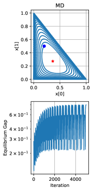
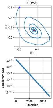
Figure 1: Dyanmics on a simple $3$-dimensional preference game. The unique Nash equilibrium is $[4/11,3/11,4/11]$ represented as red star. We initialize all algorithms at the blue dot point $[0.2,0.5,0.3]$.

Experiments using noiseless gradient

We present numerical results of mirror-descent (MD) algorithms (equivalent to MWU) and COMAL (Algorithm 1) in Figure 1. We can see that the MD algorithm diverges from the unique Nash equilibrium and suffers a large equilibrium gap, while COMAL achieves fast last-iterate convergence to the Nash equilibrium, aligned with our theoretical results (Theorem 1).

Experiements using preference samples

Since the popular iterative DPO algorithm does not contain a gradient step, we also conduct experiments with only Oracle query access to the preference model. We compare the performance of various algorithms, including iterative DPO, iterative IPO, SPPO, and INPO and present results in Figure 2. The sample-only setting is also more aligned with what happens in practice. We use a sufficient number of samples in each iteration for every algorithm. As a result, the COMAL performs the same as in the noiseless gradient setting, while the iterative IPO algorithm becomes equivalent to the MD algorithm. We note the following:

Iterative DPO: We observe that iterative DPO diverges and cycles between extreme policies (e.g., outputting $y_{a}$ with probability close to $1$). This is aligned with  (Azar et al., 2024), where they found DPO will converge to the deterministic policy regardless of the regularization parameter in extreme preference settings. The cycling behavior of iterative DPO may be explained as follows: in each iteration, DPO converges to a nearly deterministic policy output $y$; then the new preference data shows that $y^{\prime}\neq y$ is more preferred; finally, iterative DPO cycles over $\mathcal{Y}$ since the preference itself exhibits a cycle and there is no clear winner.

Iterative IPO (Azar et al., 2024; Calandriello et al., 2024): The IPO loss is a variant of the DPO loss, but it does not rely on the BT model assumption and works for a general preference model. However, as we have discussed before, (exactly) minimizing the IPO loss is equivalent to performing one MD step, and thus, iterative IPO is equivalent to MD up to sampling error. As a result, we observe that iterative IPO also exhibits cycling behavior.

SPPO (Wu et al., 2024): The SPPO algorithm (see Appendix D) is not exactly the same as MWU since SPPO assumes the partition function is always $Z=\log\frac{\eta}{2}$ which may not be the case. We observe that SPPO exhibits very similar cycling behavior as MD. We conclude that SPPO approximates MD very well in this instance and exhibits similar behavior.

INPO (Zhang et al., 2024): The INPO algorithm is designed for finding the Nash equilibrium of the KL regularized game $J_{\tau}(\pi_{1},\pi_{2},\pi_{\mathrm{ref}})$. As we proved in Theorem 2, INPO does not diverge and exhibits last-iterate convergence. However, it converges to a point that differs from the Nash equilibrium of the game $J(\pi_{1},\pi_{2})$ and, as a result, lacks the robust alignment property.

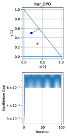
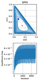
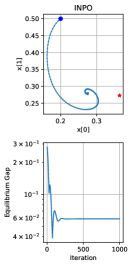
Figure 2: Dyanmics on a simple $3$-dimensional preference game. The unique Nash equilibrium is $[4/11,3/11,4/11]$ represented as red star. We initialize all algorithms at the blue dot point $[0.2,0.5,0.3]$.

5 LLM-Based Experiments

Apart from the controlled synthetic experiments, we conduct experiments with a pre-trained LLM, Qwen2-1.5B (Yang et al., 2024), on a commonly used dataset UltraFeedback (Cui et al., 2023) to show the effectiveness of COMAL under the practical preference optimization setting.

5.1 Experimental Settings

Datasets We use the UltraFeedback dataset, specifically its binarized version for preference fine-tuning. It contains 64K data examples consisting of a user instruction and a positive-negative output pair annotated by GPT-4. The instructions in this dataset span a wide range of types, making it well-suited for studying preference optimization in practical settings. Since we focus on online and iterative preference optimization, only the instructions are used because the output pairs will be generated and annotated online. In addition, to reduce the computational cost, the instructions are randomly split into 6 equal-size subsets. Each subset therefore contains around 10K instructions and is used in one training iteration.

Preference Oracle The preference oracle we used is Llama-3-OffsetBias-8B (Park et al., 2024), which is a pairwise preference model that predicts which output is better given an instruction and a pair of outputs. Fine-tuned from Meta-Llama-3-8B-Instruct (Dubey et al., 2024), it achieves strong performance on various human preference alignment benchmarks in RewardBench (Lambert et al., 2024). We selected it as the preference oracle for its balance of computational efficiency and alignment with human preferences, making it suitable for iterative preference optimization.

Preference Data Generation To construct the preference data, i.e., output pairs with a preference annotation specifying which one is better, we adopt the setting of Zhang et al. (2024) by sampling 5 candidate outputs for each instruction with a temperature of 0.8 and applying the preference oracle to compare all the output pairs constructed. The best and the worst candidate outputs, derived from the pairwise comparison results, are then selected to form a data point.

Baselines We include the following baselines for comparisons with COMAL: (1) SFT, which fine-tunes the pre-trained Qwen2-1.5B on the UltraChat dataset, with the resulting checkpoint serving as the starting point and/or reference policy for the other training algorithms; (2) vanilla DPO (Rafailov et al., 2024) and (3) vanilla IPO (Azar et al., 2024), where one training iteration is performed over the entire instruction set of UltraFeedback with output pairs sampled from the SFT policy; (4) INPO (Zhang et al., 2024), where each iteration of training is performed on a single data split; (5) iterative IPO, which follows a training setting similar to INPO but without the KL regularization with respect to the reference policy.

Evaluations We use the instructions in a widely used benchmark, AlpacaEval (Li et al., 2023), to construct the test set, since these instructions are diverse and cover various task scenarios. However, instead of using GPT-4, the default evaluator for the AlpacaEval benchmark, we chose to use the same preference oracle used during data generation, Llama-3-OffsetBias-8B, as the evaluator. This decision was made to maintain a controlled experimental setting, ensuring that the preference oracle the model learns to fit is also the one used to evaluate its performance.

Training Details We follow the training recipe proposed in Tunstall et al. (2023) for the experiments. Specifically, at each training iteration, the models are fine-tuned for 3 epochs with a batch size of 32 and maximum learning rate of $5\times 10^{-7}$, using a linear learning rate scheduler where 10% of the steps are for warmup and the rest for linearly decreasing the rate. The checkpoints are selected based on their validation loss on the UltraFeedback dataset. The training is performed on 8 NVIDIA A6000 Ada GPUs with 48GB memory, and one training iteration over the 10K instructions takes around 5 hours. Due to the relatively high computational requirements and the large number of training iterations we tested (up to 42), we opted to use a moderately sized LLM and did not conduct an exhaustive hyper-parameter search, instead referencing settings from previous work when appropriate. To the best of our knowledge, multi-iteration training like ours has rarely been explored in previous work. For example, INPO (Zhang et al., 2024) only performed optimization for up to 3 iterations, which is equivalent to just one full round over UltraFeedback’s instructions.

Hyper-Parameters We conduct a grid search for the strength of the KL regularization, $\eta^{-1}$, in both vanilla DPO and IPO. We found that DPO achieves the best performance when $\eta^{-1}$ is set to 0.01, while IPO achieves the best performance when $\eta^{-1}$ is set within the range of 0.002 - 0.01. We then choose the value of $\eta^{-1}$ to be 0.002 to encourage larger learning steps. This value of $\eta$ is also used for iterative IPO. For INPO, we compare two settings where $\eta^{-1}$ is set to 0.002 and 0.01, corresponding to a small and a large regularization respectively. INPO has another hyper-parameter $\tau$ which controls the strength of the KL regularization from the reference policy. We determine its value following the setting of Zhang et al. (2024), where $\eta\tau$ is set to a fixed ratio, $1/3$. Regarding COMAL, which is implemented based on INPO as outlined in Algorithm 4, $\eta^{-1}$ is also set to 0.002 at the beginning of the training. The reference policy used in COMAL is updated when the first optimization step begins to converge or overfit, and $\eta^{-1}$ is increased to 0.01 to improve training stability.

5.2 Result Analysis

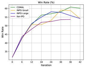
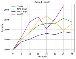
Figure 3: Comparisons of Iterative IPO (Iter-IPO), INPO, and COMAL. The average win rates of the trained checkpoints against the best checkpoints of each training algorithm, and the average lengths of the outputs are compared. For INPO, two variations with a small regularization ($\eta^{-1}=0.002$, INPO-Small) and a large regularization ($\eta^{-1}=0.01$, INPO-Large) are compared.

Figure 3 presents the training dynamics of three iterative preference optimization algorithms we compared: iterative IPO (Iter-IPO), INPO with a small and a large regularization (INPO-Small and INPO-Large), and COMAL, which are demonstrated by their checkpoints’ win rates against the best checkpoints produced by 7 different algorithms: SFT, IPO, DPO, Iter-IPO, INPO-Small, INPO-Large, COMAL, and the average lengths of their outputs. For INPO and COMAL, the model is trained for up to 42 iterations, equivalent to 7 training rounds over the entire instruction set since it has been split into 6 subsets. We note that:

(1) Iter-IPO shows a quicker improvement rate at the beginning of the training, but its performance begins to lag behind other algorithms after the first training round with a rapid increase in output length, which indicates the inherent instability of this training algorithm.

(2) INPO achieves stronger performance and larger improvement rates compared to Iter-IPO. However, the win rates of both INPO-Small and INPO-Large start to decrease after 5 training rounds. We suspect this suggests that INPO has started to converge and/or overfit. Moreover, for INPO-Small, its performance shows only a minor improvement and even a slight decline during training rounds 2 to 4 (iterations 12 - 24). Therefore, for COMAL, which shares the same training trajectory as INPO-Small for the first two training rounds, we update the reference policy at the beginning of the third training round, following the optimization process described in Algorithm 4.

(3) COMAL is able to further improve the model performance with the updated reference policy. Notably, its performance continues to improve up until the 6th training round, when the other algorithms begin to degrade, demonstrating the benefit of updating the reference policy.

Table 2 provides pairwise comparisons between the best checkpoints of the iterative preference optimization algorithms and a few baselines. It demonstrates the clear advantage of COMAL, which is able to achieve a win rate that is strictly above 50% against all the other checkpoints. The comparison of the final checkpoints of different algorithms after the last iteration is presented in Appendix H, where COMAL is able to achieve significantly better performance thanks to its stability.

Table 2: Performance comparison of different training algorithms. The row v.s. column win rate (%) is reported. The best checkpoints produced by each training algorithm are compared. For INPO, we report two variations with a small regularization ($\eta^{-1}=0.002$, INPO-Small) and a large regularization ($\eta^{-1}=0.01$, INPO-Large).

Row/Column	SFT	DPO	IPO	Iter-IPO	INPO-Large	INPO-Small	COMAL	Avg
Iter-IPO	67.33	62.36	58.76	50.00	48.20	44.72	44.10	53.64
INPO-Large	77.02	69.81	67.83	51.80	50.00	46.21	44.84	58.22
INPO-Small	73.66	66.21	66.46	55.28	53.79	50.00	48.70	59.16
COMAL	74.53	70.56	68.82	55.90	55.16	51.30	50.00	60.90

6 Related Work

Alignment under Preference models

Most existing approaches adopt the Bradley-Terry (BT) preference model (Bradley and Terry, 1952; Christiano et al., 2017), which involves first learning a preference model and then optimizing the objective function with a KL divergence penalty relative to the original language model. For example, RLHF (Ouyang et al., 2022) aims to ensure that LLMs follow instructions by initially learning a BT model and subsequently fine-tuning the model based on the learned reward while regularizing it with the original LLM.

Building on this framework, Rafailov et al. (2024) introduces Direct Preference Optimization (DPO) that maintains the assumption of the BT model for preferences but eliminates the preference learning step by reformulating the objective and optimizing it directly. Additionally, Ethayarajh et al. (2024) diverges from the traditional BT-based methods by deriving algorithms that bypass the preference modeling step altogether. Instead, they model user preferences based on Kahneman and Tversky’s utility theory.

Alignment Solution Concepts under General Preferences

Azar et al. (2024) is the first to consider general preferences. They propose the IPO algorithm, an offline algorithm that directly optimizes the win rate of the model penalized by the KL divergence with respect to the original model. Munos et al. (2024) also consider general preferences and aim to find the von Neumann winner, which corresponds to the Nash equilibrium of a game played between the two LLMs over the win rate. They propose a variant of the Mirror Descent (MD) algorithm called Nash-MD and show last-iterate convergence in the KL-regularized game. Concurrently, Swamy et al. (2024) study the same solution concept focusing more on sequential games. Calandriello et al. (2024) proved that the objective of the the IPO algorithm coincides with the Nash policy under a proper choice of the parameter that controls the regularization.

Iterative Self-Play Algorithms

Apart from the aforementioned works, recent research has also proposed practical implementations of Mirror Descent (MD) algorithms, which can be used to learn Nash equilibria through self-play. Rosset et al. (2024) propose Direct Nash Optimization (DNO), where, at each iteration, the model regresses predicted preferences against actual preferences using cross-entropy loss. Similarly, Wu et al. (2024) introduces the Self-Play Preference Optimization (SPPO) method, Gao et al. (2024) introduces Reinforcement Learning via Regressing Relative Rewards (REBEL), and Richemond et al. (2024) introduces the Direct Reward Optimization (DRO) which regresses the loss using the $\ell_{2}$ distance at each iteration. Since these algorithms simulate the MD update, when applied in a two-player zero-sum game, they only have average-iterate convergence but all diverge in the last iterate. Moreover, all these methods require the estimation of the win rate, which can be computationally expensive.

Most closely related to our work is Iterative Nash Policy Optimization (INPO) by Zhang et al. (2024), which continues to use $\ell_{2}$ distance regression. However, by further reformulating and simplifying the objective in a manner similar to IPO, INPO eliminates the need to estimate the expected win rate. The primary distinction between our approach and INPO is that INPO is designed for the KL-regularized game and is equivalent to MD; while our algorithm COMAL is inspired by the Conceptual Prox algorithm and guarantees last-iterate convergence in the original game. This fundamental difference allows COMAL to achieve more favorable convergence properties and outperform INPO, achieving a win rate strictly greater than 50% against it.

Last-Iterate Convergence in Games

Mirror Descent fails to converge in simple zero-sum games, often resulting in cycling behavior (Mertikopoulos et al., 2018). In contrast, several algorithms have been shown to achieve last-iterate convergence including the Proximal Point (PP) method (Rockafellar, 1976), Extra-Gradient (EG) (Korpelevich, 1976), Optimistic Gradient Descent (OGD) (Popov, 1980; Rakhlin and Sridharan, 2013), and the Conceptual Prox/Mirror Prox methods (Nemirovski, 2004). The asymptotic convergence properties of these algorithms have been extensively studied (Popov, 1980; Facchinei and Pang, 2003; Iusem et al., 2003; Nemirovski, 2004; Daskalakis and Panageas, 2018). Recently, there has been a growing focus on establishing finite-time convergence guarantees for these methods, addressing the practical necessity of understanding their performance within a limited number of iterations (see e.g., (Mokhtari et al., 2020b, a; Golowich et al., 2020b, a; Bauschke et al., 2021; Wei et al., 2021; Cai et al., 2022; Gorbunov et al., 2022; Cai and Zheng, 2023a, b; Cai et al., 2023, 2024b, 2024a) and references therein).

7 Conclusion

We have proposed COMAL, a meta-algorithm for preference optimization that provably converges to the Nash equilibrium policy in the last iterate. We have provided a theoretical analysis of the properties of COMAL and have empirically demonstrated its effectiveness under both synthetic and real-world experimental settings. We believe COMAL has significant potential to enhance the performance of LLMs in the alignment fine-tuning setting, due to its theoretical guarantees and flexibility, as it can be integrated with existing learning algorithms while overcoming their limitations.

Appendix A Properties of the Prox Operator

Recall that $\operatorname{Prox}(z,g)=\operatorname*{argmax}_{z^{\prime}\in\mathcal{Z}}{\mathchoice{\left\langle g,z^{\prime}\right\rangle}{\langle g,z^{\prime}\rangle}{\langle g,z^{\prime}\rangle}{\langle g,z^{\prime}\rangle}}-D_{\varphi}(z^{\prime}||z)=\operatorname*{argmax}_{z^{\prime}\in\mathcal{Z}}{\mathchoice{\left\langle g+\nabla\varphi(z),z^{\prime}\right\rangle}{\langle g+\nabla\varphi(z),z^{\prime}\rangle}{\langle g+\nabla\varphi(z),z^{\prime}\rangle}{\langle g+\nabla\varphi(z),z^{\prime}\rangle}}-\varphi(z^{\prime})$. The following properties of the prox operator are well-known in the literature(e.g., [Nemirovski, 2004])

Lemma 1.

$\operatorname{Prox}(z,g)=z^{\prime}$ if and only if ${\mathchoice{\left\langle g+\nabla\varphi(z)-\nabla\varphi(z^{\prime}),z^{\prime}-z^{*}\right\rangle}{\langle g+\nabla\varphi(z)-\nabla\varphi(z^{\prime}),z^{\prime}-z^{*}\rangle}{\langle g+\nabla\varphi(z)-\nabla\varphi(z^{\prime}),z^{\prime}-z^{*}\rangle}{\langle g+\nabla\varphi(z)-\nabla\varphi(z^{\prime}),z^{\prime}-z^{*}\rangle}}\geq 0$ for all $z^{*}\in\mathcal{Z}$.

Corollary 1.

Let $\operatorname{Prox}(z,g)=z^{\prime}$, then

$${\mathchoice{\left\langle g,z^{*}-z^{\prime}\right\rangle}{\langle g,z^{*}-z^{\prime}\rangle}{\langle g,z^{*}-z^{\prime}\rangle}{\langle g,z^{*}-z^{\prime}\rangle}}\leq D_{\varphi}(z^{*}||z)-D_{\varphi}(z^{*}||z^{\prime})-D_{\varphi}(z^{\prime}||z),\quad\forall z^{*}\in\mathcal{Z}$$

Appendix B Proof of Theorem 1

The proof of Theorem 1 is largely inspired by existing results for the conceptual prox algorithm in the literature [Facchinei and Pang, 2003, Nemirovski, 2004]. We first consider the case where each step of COMAL, $\pi^{t+1}\leftarrow\operatorname*{argmax}_{\pi_{1}}\min_{\pi_{2}}J_{\tau}(\pi_{1},\pi_{2},\pi_{\mathrm{ref}})$, can be solved exactly in Section B.1. We then extend the proof to the case where we only solve the regularized game approximately in Section B.2. In both cases, we prove last-iterate convergence to Nash equilibrium, i.e., $\lim_{t\rightarrow\infty}\pi^{t}$ exists and is a Nash equilibrium. The proof for the latter case seems to be the first in the literature.

In Theorem 1, we make the following assumption.

Assumption 1.

We assume there exists a Nash equilibrium $\pi^{\star}$ such that $\mathrm{supp}(\pi^{\star})=\mathrm{supp}(\pi_{\mathrm{sft}})$.

This assumption is mild and much weaker than the “Bounded Log Density" assumptions used in previous works [Rosset et al., 2024, Zhang et al., 2024], which directly assumes $|\log\frac{\pi^{t}}{\pi_{\mathrm{sft}}}|$ is bounded.

B.1 Last-Iterate Convergence under Exact Solutions

Recall that $\Pi:=\{\pi:\mathrm{supp}(\pi)\subseteq\mathrm{supp}(\pi_{\mathrm{sft}})\}$. Then $\operatorname{KL}(\pi||\pi_{\mathrm{sft}})\leq D:=\max_{y:\pi_{\mathrm{sft}}(y)>0}\log\pi_{\mathrm{sft}}(y)$ is bounded for any $\pi\in\Pi$. We first prove $\operatorname{KL}(\pi^{\star}||\pi^{t+1})\leq\operatorname{KL}(\pi^{\star}||\pi^{t})$ for any $t\geq 1$.

Lemma 2.

Let $\pi^{\star}$ be an Nash equilibrium of $J(\pi_{1},\pi_{2})$. Then for any $\tau>0$, if

$$(\pi,\pi)=\operatorname*{argmax}_{\pi_{1}\in\Pi}\operatorname*{argmin}_{\pi_{2}\in\Pi}J_{\tau}(\pi_{1},\pi_{2},\pi_{\mathrm{ref}}),$$

then

$$\operatorname{KL}(\pi^{\star}||\pi)\leq\operatorname{KL}(\pi^{\star}||\pi_{\mathrm{ref}})-\operatorname{KL}(\pi||\pi_{\mathrm{ref}})$$

Proof.

By definition of the prox operator, we have

$$\pi =\operatorname*{argmax}_{\pi_{1}\in\Pi}J_{\tau}(\pi_{1},\pi,\pi_{\mathrm{ref}})$$

$$=\operatorname*{argmax}_{\pi_{1}\in\Pi}\mathbb{P}(\pi_{1}\succ\pi)-\tau\operatorname{KL}(\pi_{1},\pi_{\mathrm{ref}})$$

$$=\operatorname{Prox}(\pi_{\mathrm{ref}},\frac{1}{\tau}\mathbb{P}(\cdot\succ\pi)).$$ (7)

Using Corollary 1, we have for any $\pi^{\prime}\in\Pi$,

$$\frac{1}{\tau}{\mathchoice{\left(\mathbb{P}(\pi^{\prime}\succ\pi)-\mathbb{P}(\pi\succ\pi)\right)}{(\mathbb{P}(\pi^{\prime}\succ\pi)-\mathbb{P}(\pi\succ\pi))}{(\mathbb{P}(\pi^{\prime}\succ\pi)-\mathbb{P}(\pi\succ\pi))}{(\mathbb{P}(\pi^{\prime}\succ\pi)-\mathbb{P}(\pi\succ\pi))}}\leq\operatorname{KL}(\pi^{\prime}||\pi_{\mathrm{ref}})-\operatorname{KL}(\pi^{\prime}||\pi)-\operatorname{KL}(\pi||\pi_{\mathrm{ref}}).$$ (8)

Plugging $\pi^{\prime}=\pi^{\star}$ into the above inequality and noting that $\mathbb{P}(\pi\succ\pi)=\frac{1}{2}$, we get

$$\frac{1}{\tau}{\mathchoice{\left(\mathbb{P}(\pi^{\star}\succ\pi)-\frac{1}{2}\right)}{(\mathbb{P}(\pi^{\star}\succ\pi)-\frac{1}{2})}{(\mathbb{P}(\pi^{\star}\succ\pi)-\frac{1}{2})}{(\mathbb{P}(\pi^{\star}\succ\pi)-\frac{1}{2})}}\leq\operatorname{KL}(\pi^{\star}||\pi_{\mathrm{ref}})-\operatorname{KL}(\pi^{\star}||\pi)-\operatorname{KL}(\pi||\pi_{\mathrm{ref}}).$$

Since $\pi^{\star}$ is a Nash equilibrium and thus $\mathbb{P}(\pi^{\star}\succ\pi)\geq\frac{1}{2}$, the lefthand side of the above inequality is $\geq 0$. Then we have

$$\operatorname{KL}(\pi^{\star}||\pi)\leq\operatorname{KL}(\pi^{\star}||\pi_{\mathrm{ref}})-\operatorname{KL}(\pi||\pi_{\mathrm{ref}}).$$

∎

Lemma 2 implies the following properties on the trajectory $\{\pi^{t}\}$.

Corollary 2.

Denote $\pi^{\star}$ an Nash equilibrium such that $\mathrm{supp}(\pi^{\star})=\mathrm{supp}(\pi_{\mathrm{sft}})$ as guaranteed by 1. Then the following holds for the trajectory $\{\pi^{t}\}$ produced by COMAL:

• $\operatorname{KL}(\pi^{\star}||\pi^{t+1})\leq\operatorname{KL}(\pi^{\star}||\pi^{t})$ for all $t\geq 1$.

• $\sum_{t=1}^{\infty}\operatorname{KL}(\pi^{t+1}||\pi^{t})\leq\operatorname{KL}(\pi^{\star}||\pi_{\mathrm{sft}})<+\infty$.

• For all $t\geq 1$, it holds that for $y\in\mathrm{supp}(\pi_{\mathrm{sft}})$, $\pi^{t}(y)\geq c>0$ where $c$ is some constant $c$ depends only on $\pi^{\star}$ and $\pi_{\mathrm{sft}}$. This also holds even for any limit point of $\{\pi^{t}\}$.

Proof.

The first item is direct from Lemma 2. The second item is also direct by applying Lemma 2 for $t\geq 1$:

$$\sum_{t=1}^{\infty}\operatorname{KL}(\pi^{t+1}||\pi^{t})\leq\sum_{t=1}^{\infty}\operatorname{KL}(\pi^{\star}||\pi^{t})-\operatorname{KL}(\pi^{\star}||\pi^{t+1})\leq\operatorname{KL}(\pi^{\star}||\pi_{\mathrm{sft}})\leq D<\infty.$$

Now we consider the third item. Define $D:=\operatorname{KL}(\pi^{\star}||\pi_{\mathrm{sft}})$ and $p_{\min}:=\min_{y\in\mathrm{supp}(\pi^{\star})}\pi^{\star}(y)$. By 1, $p_{\min}>0$. Then

$$\operatorname{KL}(\pi^{\star}||\pi^{t})\leq D \Rightarrow p_{\min}\log\frac{p_{\min}}{\pi^{t}(y)}\leq D,\forall y\in\mathrm{supp}(\pi^{\star})$$

$$\Rightarrow\pi^{t}(y)\geq\frac{p_{\min}}{\exp(D/p_{\min})},\forall y\in\mathrm{supp}(\pi^{\star}).$$

Since the above holds for all $\pi^{t}$, it also holds for any limit point of $\{\pi^{t}\}$. ∎

Since the sequence $\{\pi^{t}\}$ is bounded (all lies in the simplex), it has at least one limit point $\hat{\pi}$. The next lemma shows that a limit point must be a Nash equilibrium.

Lemma 3.

If $\hat{\pi}$ is a limit point of $\{\pi^{t}\}$, then $\hat{\pi}$ is a Nash equilibrium of $J(\pi_{1},\pi_{2})$.

Proof.

By item 2 in Corollary 2, we have $\lim_{t\rightarrow\infty}\operatorname{KL}(\pi^{t+1}||\pi^{t})=0$. This implies $\lim_{t\rightarrow\infty}{\mathchoice{\left\|\pi^{t+1}-\pi^{t}\right\|}{\|\pi^{t+1}-\pi^{t}\|}{\|\pi^{t+1}-\pi^{t}\|}{\|\pi^{t+1}-\pi^{t}\|}}=0$. As $\hat{\pi}$ is a limit point of $\{\pi^{t}\}$, we let $\{\pi^{k}:k\in\kappa\}$ be the subsequence that converges to $\hat{\pi}$. Then by Section B.1, we have

$$\lim_{k\in\kappa,k\rightarrow\infty}\pi^{k+1}=\lim_{k\in\kappa,k\rightarrow\infty}\operatorname{Prox}(\pi^{k},\frac{1}{\tau}\mathbb{P}(\cdot\succ\pi^{k+1}))$$

$$\Rightarrow \hat{\pi}=\operatorname{Prox}(\hat{\pi},\frac{1}{\tau}\mathbb{P}(\cdot\succ\hat{\pi})).$$

Thus $\hat{\pi}$ is a fixed point of $\operatorname{Prox}(\pi,\frac{1}{\tau}\mathbb{P}(\cdot\succ\pi)$. Moreover, by item 3 in Corollary 2, we have $\mathrm{supp}(\hat{\pi})=\mathrm{supp}(\pi_{\mathrm{sft}})$. Now consider both the max and min player running MWU initialized with $\pi^{1}=\hat{\pi}$. Then we have $\pi^{t}=\hat{\pi}$ for all $t\geq 1$. By Equation 8, we have for any $\pi^{\prime}\in\Pi$,

$$\frac{1}{\tau}\sum_{t=1}^{\infty}{\mathchoice{\left(\mathbb{P}(\pi^{\prime}\succ\hat{\pi})-\frac{1}{2}\right)}{(\mathbb{P}(\pi^{\prime}\succ\hat{\pi})-\frac{1}{2})}{(\mathbb{P}(\pi^{\prime}\succ\hat{\pi})-\frac{1}{2})}{(\mathbb{P}(\pi^{\prime}\succ\hat{\pi})-\frac{1}{2})}}\leq\operatorname{KL}(\pi^{\prime}||\hat{\pi})<\infty,$$

where the inequality holds since $\mathrm{supp}(\pi^{\prime})\subseteq\mathrm{supp}(\hat{\pi})$. As a result, we get

$$\mathbb{P}(\pi^{\prime}\succ\hat{\pi})\leq\frac{1}{2},\forall\pi^{\prime}\in\Pi\Leftrightarrow\mathbb{P}(\hat{\pi}\succ\pi^{\prime})\geq\frac{1}{2},\forall\pi^{\prime}\in\Pi$$

Thus $\hat{\pi}$ is a Nash equilibrium of $J(\pi_{1},\pi_{2})$. ∎

Proof of Theorem 1

By Lemma 3, we know a limit point $\hat{\pi}$ is a Nash equilibrium. Then by Corollary 2, $\{\operatorname{KL}(\hat{\pi}||\pi^{t})\geq 0\}$ is a decreasing sequence. Thus $\{\operatorname{KL}(\hat{\pi}||\pi^{t})\}$ converges. Let $\{\pi^{k}:k\in\kappa\}$ be a subsequence that converges to $\hat{\pi}$. Then we have

$$\lim_{t\rightarrow\infty}\operatorname{KL}(\hat{\pi}||\pi^{t})=\lim_{k\in\kappa,k\rightarrow\infty}\operatorname{KL}(\hat{\pi}||\pi^{k})=\operatorname{KL}(\hat{\pi}||\hat{\pi})=0.$$

Thus we have $\lim_{t\rightarrow\infty}\pi^{t}=\hat{\pi}$ is a Nash equilibrium. This completed the proof of Theorem 1.

B.2 Last-Iterate Convergence under Approximate Solutions

This section considers the case where we can not solve the regularized game $J_{\tau}(\pi_{1},\pi_{2},\pi_{\mathrm{ref}})$ exactly but only compute an approximate solution. Specifically, we consider the following inexact COMAL update: denote $\hat{\pi}^{t+1}=\operatorname*{argmax}_{\pi_{1}\in\Pi}\min_{\pi_{2}\in\Pi}J_{\tau}(\pi_{1},\pi_{2},\pi^{t})$ the exactly solution; the algorithm updates the next iterate $\pi^{t+1}$ as an $\varepsilon_{t}$-approximate solution such that

$$\operatorname{KL}(\hat{\pi}^{t+1},\pi^{t+1})\leq\varepsilon_{t}=O{\mathchoice{\left(\frac{1}{t^{4}}\right)}{(\frac{1}{t^{4}})}{(\frac{1}{t^{4}})}{(\frac{1}{t^{4}})}}.$$ (9)

We note that we can compute $\pi^{t+1}$ within $\varepsilon_{t}$ error using $O(\log\frac{1}{\varepsilon_{t}})=O(\log t)$ iterations of Algorithm 2 (Theorem 2).

We denote $\Pi^{\star}$ the set of Nash equilibria such that each $\pi^{\star}\in\Pi^{\star}$ has support $\mathrm{supp}(\pi^{\star})=\mathrm{supp}(\pi_{\mathrm{sft}})$ as guaranteed by 1. We introduce a few quantities that depend on the Nash equilibria and the initial policy.

Definition 4.

We define the following constants.

1. $p_{\mathrm{sft}}:=\max\{p>0:\forall y\in\mathrm{supp}(\pi_{\mathrm{sft}}),\pi_{\mathrm{sft}}(y)\geq p\}$; $D:=|\mathcal{Y}|\log\frac{1}{p_{\mathrm{sft}}}$ so that $\operatorname{KL}(\pi||\pi_{\mathrm{sft}})\leq D$ for all $\pi\in\Pi$

2. $p_{\min}:=\max\{p>0:\exists\pi^{\star}\in\Pi^{\star},\forall y\in\mathrm{supp}(\pi_{\mathrm{sft}}),\pi^{\star}(y)\geq p\}$; Let $\pi^{\star}\in\Pi^{\star}$ be a Nash equilibrium so that $\pi^{\star}(y)\geq p_{\min}$ holds for all $y$ in its support.

3. $c_{1}:=\frac{p_{\min}}{\exp{(D+2)/p_{\min}}}$ and $c_{2}:=\frac{c_{1}}{\exp(1/c_{1})}$.

Our main result is that if each optimization problem at iteration $t$ can be solved within approximation error $\varepsilon_{t}\leq\frac{c_{1}}{3t^{2}}$, then COMAL converges in last-iterate to a Nash equilibrium.

Theorem 3 (COMAL with approximate regularized game solver).

Assume 1 holds. If in each iteration $t\geq 1$, the returned iterate $\pi^{t+1}$ is an $\varepsilon_{t}$-approximate solution to $J_{\tau}(\pi_{1},\pi_{2},\pi^{t})$ as defined in (9) with $\varepsilon_{t}\leq\frac{c_{1}^{2}}{9t^{4}}$ ($c_{1}$ defined in Definition 4), then $\{x^{t}\}$ converges to a Nash equilibrium of $J(\pi_{1},\pi_{2})$.

We need the following technical lemma in the proof of Theorem 3.

Lemma 4.

Let $\varepsilon_{t}\leq\frac{c_{1}^{2}}{9t^{4}}$. Then for all $t\geq 1$,

1. $\operatorname{KL}(\pi^{\star}||\pi^{t+1})\leq\operatorname{KL}(\pi^{\star}||\pi^{t})-\operatorname{KL}(\pi^{t+1}||\pi^{t})+\frac{1}{t^{2}}$.

2. $\min_{y\in\mathrm{supp}(\pi_{\mathrm{sft}})}\pi^{t}(y)\geq c_{2}$.

3. $\lim_{t\rightarrow\infty}{\mathchoice{\left\|\pi^{t+1}-\pi^{t}\right\|}{\|\pi^{t+1}-\pi^{t}\|}{\|\pi^{t+1}-\pi^{t}\|}{\|\pi^{t+1}-\pi^{t}\|}}=0$.

4. For any Nash equilibrium $\hat{\pi}\in\Pi$ and $t\geq 1$, we have $\operatorname{KL}(\hat{\pi}||\pi^{t+1})\leq\operatorname{KL}(\hat{\pi}||\pi^{t})+\frac{1}{t^{2}}$

Proof.

By Lemma 2, we have $\hat{\pi}^{t+1}=\operatorname{Prox}(\pi^{t},\mathbb{P}(\cdot\succ\hat{\pi}^{t+1}))$ and

$$\operatorname{KL}(\pi^{\star}||\hat{\pi}^{t+1})\leq\operatorname{KL}(\pi^{\star}||\pi^{t})-\operatorname{KL}(\hat{\pi}^{t+1}||\pi^{t}).$$ (10)

The above implies

$$\operatorname{KL}(\pi^{\star}||\pi^{t+1}) \leq\operatorname{KL}(\pi^{\star}||\pi^{t})-\operatorname{KL}(\pi^{t+1}||\pi^{t})+\underbrace{\operatorname{KL}(\pi^{\star}||\pi^{t+1})-\operatorname{KL}(\pi^{\star}||\hat{\pi}^{t+1})}_{E_{1}}$$

$$+\underbrace{\operatorname{KL}(\pi^{t+1}||\pi^{t})-\operatorname{KL}(\hat{\pi}^{t+1}||\pi^{t})}_{E_{2}}.$$ (11)

Now, we use induction to prove the claim. For the base case, we define $\pi^{0}:=\pi^{1}$ and $\varepsilon_{t}=0$, then

Base Case: $t=0$

Since $\pi^{0}=\pi^{1}$, we have $\operatorname{KL}(\pi^{1}||\pi^{0})=0$. Then it is clear that

$$\operatorname{KL}(\pi^{\star}||\pi^{1})\leq\operatorname{KL}(\pi^{\star}||\pi^{0})-\operatorname{KL}(\pi^{1}||\pi^{0}).$$

Moreover, by Proposition 1 and $D\geq\operatorname{KL}(\pi^{\star}||\pi_{\mathrm{sft}})$, we have $\min_{y\in\mathrm{supp}(\pi^{1})}\pi^{1}(y)\geq c_{1}\geq c_{2}$.

Induction: $t\geq 1$

We have

$$\operatorname{KL}(\pi^{\star}||\hat{\pi}^{t+1}) \leq\operatorname{KL}(\pi^{\star}||\pi^{t})$$ ((10))

$$\leq\operatorname{KL}(\pi^{\star}||\pi_{\mathrm{sft}})+\sum_{t=1}^{t-1}\frac{1}{t^{2}}$$ (inductive hypothesis)

$$\leq D+2. D\geq\operatorname{KL}(\pi^{\star}||\pi_{\mathrm{sft}})$$ ()

Using Proposition 1, we have $\min_{y\in\mathrm{supp}(\pi_{\mathrm{sft}})}\hat{\pi}^{t+1}(y)\geq c_{1}$. By $\operatorname{KL}(\hat{\pi}^{t+1}||\pi^{t+1})\leq\varepsilon_{t}\leq 1$ and Proposition 1 again, we get $\min_{y\in\mathrm{supp}(\pi_{\mathrm{sft}})}\pi^{t+1}(y)\geq c_{2}:=\frac{c_{1}}{\exp(1/c_{1})}$. Thus, both $\hat{\pi}^{t+1}$ and $\pi^{t+1}$ are bounded away from the boundary in their support. Further by $\operatorname{KL}(\hat{\pi}^{t+1}||\pi^{t+1})\leq\varepsilon_{t}$, we have

$$\sum_{y}\hat{\pi}^{t+1}(y)\log\frac{\hat{\pi}^{t+1}(y)}{\pi^{t+1}(y)}\leq\varepsilon_{t}\Rightarrow\max_{y}\log\frac{\hat{\pi}^{t+1}(y)}{\pi^{t+1}(y)}\leq\frac{\varepsilon_{t}}{c_{1}}.$$

As a result, we can bound

$$E_{1} =\operatorname{KL}(\pi^{\star}||\pi^{t+1})-\operatorname{KL}(\pi^{\star}||\hat{\pi}^{t+1})$$

$$=\sum_{y}\pi^{\star}(y)\log\frac{\hat{\pi}^{t+1}(y)}{\pi^{t+1}(y)}$$

$$\leq\max_{y}\log\frac{\hat{\pi}^{t+1}(y)}{\pi^{t+1}(y)}$$

$$\leq\frac{\varepsilon_{t}}{c_{1}}.$$

Moreover, we have

$$E_{2} =\operatorname{KL}(\pi^{t+1}||\pi^{t})-\operatorname{KL}(\hat{\pi}^{t+1}||\pi^{t})$$

$$=\sum_{y}(\pi^{t+1}(y)-\hat{\pi}^{t+1}(y))\log\frac{\pi^{t+1}(y)}{\pi^{t}(y)}-\operatorname{KL}(\hat{\pi}^{t+1}||\pi^{t+1})$$

$$\leq{\mathchoice{\left\|\pi^{t+1}-\hat{\pi}^{t+1}\right\|}{\|\pi^{t+1}-\hat{\pi}^{t+1}\|}{\|\pi^{t+1}-\hat{\pi}^{t+1}\|}{\|\pi^{t+1}-\hat{\pi}^{t+1}\|}}_{1}\cdot\max_{y}|\log\frac{\pi^{t+1}(y)}{\pi^{t}(y)}|$$

$$\leq\sqrt{\operatorname{KL}(\hat{\pi}^{t+1}||\pi^{t+1})}\cdot\log\frac{1}{c_{2}}$$ (Pinsker’s Inequality)

$$\leq\frac{2\sqrt{\varepsilon_{t}}}{c_{1}}$$

Combining the above two inequalities with (B.2) and noting the fact that $\varepsilon_{t}\leq\sqrt{\varepsilon_{t}}$ gives

$$\operatorname{KL}(\pi^{\star}||\pi^{t+1})\leq\operatorname{KL}(\pi^{\star}||\pi^{t})-\operatorname{KL}(\pi^{t+1}||\pi^{t})+\frac{3\sqrt{\varepsilon_{t}}}{c_{1}}.$$

We conclude the claim since $\varepsilon_{t}\leq\frac{c_{1}^{2}}{9t^{4}}$. This completes the proof for item 1 and item 2.

For item 3, we have $\sum_{t=1}^{\infty}{\mathchoice{\left\|\pi^{t+1}-\pi^{t}\right\|}{\|\pi^{t+1}-\pi^{t}\|}{\|\pi^{t+1}-\pi^{t}\|}{\|\pi^{t+1}-\pi^{t}\|}}\leq\sum_{t=1}^{\infty}\operatorname{KL}(\pi^{t+1}||\pi^{t})\leq D+2$. Thus $\lim_{t\rightarrow\infty}{\mathchoice{\left\|\pi^{t+1}-\pi^{t}\right\|}{\|\pi^{t+1}-\pi^{t}\|}{\|\pi^{t+1}-\pi^{t}\|}{\|\pi^{t+1}-\pi^{t}\|}}=0$.

For item 4, we can use Lemma 2 and $\hat{\pi}^{t+1}=\operatorname{Prox}(\pi^{t},\mathbb{P}(\cdot\succ\hat{\pi}^{t+1}))$ to get

$$\operatorname{KL}(\hat{\pi}||\pi^{t+1}) \leq\operatorname{KL}(\hat{\pi}||\pi^{t})-\operatorname{KL}(\pi^{t+1}||\pi^{t})+\underbrace{\operatorname{KL}(\hat{\pi}||\pi^{t+1})-\operatorname{KL}(\hat{\pi}||\hat{\pi}^{t+1})}_{E_{1}}$$

$$+\underbrace{\operatorname{KL}(\pi^{t+1}||\pi^{t})-\operatorname{KL}(\hat{\pi}^{t+1}||\pi^{t})}_{E_{2}}.$$ (12)

We note that $E_{2}\leq\frac{2\sqrt{\varepsilon_{t}}}{c_{1}}$ has been proved in the above. For $E_{1}$, we have

$$E_{1} =\operatorname{KL}(\hat{\pi}||\pi^{t+1})-\operatorname{KL}(\hat{\pi}||\hat{\pi}^{t+1})$$

$$=\sum_{y}\hat{\pi}(y)\log\frac{\hat{\pi}^{t+1}(y)}{\pi^{t+1}(y)}$$

$$\leq\max_{y}\log\frac{\hat{\pi}^{t+1}(y)}{\pi^{t+1}(y)}$$

$$\leq\frac{\varepsilon_{t}}{c_{1}}.$$

Thus we have $\operatorname{KL}(\hat{\pi}||\pi^{t+1})\leq\operatorname{KL}(\hat{\pi}||\pi^{t})+\frac{1}{t^{2}}$ as $\varepsilon_{t}\leq\frac{c_{1}^{2}}{9t^{4}}$. ∎

Proof of Theorem 3

Proof.

Since the sequence $\{\pi^{t}\}$ is bounded, it has at least one limit point $\hat{\pi}$. By item 2 in Lemma 4, we know $\hat{\pi}(y)\geq c_{2}$ for all $y\in\mathrm{supp}(\pi_{\mathrm{sft}})$. By item 3 in Lemma 4, we have $\lim_{t\rightarrow\infty}{\mathchoice{\left\|\pi^{t+1}-\pi^{t}\right\|}{\|\pi^{t+1}-\pi^{t}\|}{\|\pi^{t+1}-\pi^{t}\|}{\|\pi^{t+1}-\pi^{t}\|}}=0$. Denote $\{\pi^{k}:k\in\kappa\}$ a subsequence that converges to $\hat{\pi}$. Then we have

$$\hat{\pi} =\lim_{k\in\kappa,\kappa\rightarrow\infty}\pi^{k+1}$$

$$=\lim_{k\in\kappa,\kappa\rightarrow\infty}\hat{\pi}^{k+1} \operatorname{KL}(\hat{\pi}^{k+1},\pi^{k+1})\leq\varepsilon_{k} \lim_{t\rightarrow\infty}\varepsilon_{t}=0$$ ( and )

$$=\lim_{k\in\kappa,\kappa\rightarrow\infty}\operatorname{Prox}(\pi^{k},\frac{1}{\tau}\mathbb{P}(\cdot\succ\hat{\pi}^{k+1}))$$

$$=\lim_{k\in\kappa,\kappa\rightarrow\infty}\operatorname{Prox}(\pi^{k+1},\frac{1}{\tau}\mathbb{P}(\cdot\succ\hat{\pi}^{k+1})) \lim_{t\rightarrow\infty}{\mathchoice{\left\|\pi^{t+1}-\pi^{t}\right\|}{\|\pi^{t+1}-\pi^{t}\|}{\|\pi^{t+1}-\pi^{t}\|}{\|\pi^{t+1}-\pi^{t}\|}}=0$$ ()

$$=\lim_{k\in\kappa,\kappa\rightarrow\infty}\operatorname{Prox}(\pi^{k+1},\frac{1}{\tau}\mathbb{P}(\cdot\succ\pi^{k+1})) \operatorname{KL}(\hat{\pi}^{k+1},\pi^{k+1})\leq\varepsilon_{k} \lim_{t\rightarrow\infty}\varepsilon_{t}=0$$ ( and )

$$=\operatorname{Prox}(\hat{\pi},\frac{1}{\tau}\mathbb{P}(\cdot\succ\hat{\pi})).$$

Since $\hat{\pi}$ is a fixed point of $\operatorname{Prox}(\pi,\frac{1}{\tau}\mathbb{P}(\cdot\succ\pi))$ and $\mathrm{supp}(\hat{\pi})=\mathrm{supp}(\pi_{\mathrm{sft}})$, we can use the same proof in Lemma 3 to show that $\hat{\pi}$ is a Nash equilibrium of $J(\pi_{1},\pi_{2})$.

Given that $\hat{\pi}$ is a Nash equilibrium of the original game, we can apply item 4 in Lemma 4 and get

$$\operatorname{KL}(\hat{\pi}||\pi^{t+1})\leq\operatorname{KL}(\hat{\pi}||\pi^{t})+\frac{1}{t^{2}}.$$

Now we show the sequence $\{x^{t}\}$ converges to $\hat{\pi}$. Fix any $\epsilon>0$. Let $T_{1}\geq 1$ such that $\sum_{t=T_{1}}^{\infty}\frac{1}{t^{2}}<\frac{\epsilon}{2}$, Since $\hat{\pi}$ is a limit point of $\{x^{t}\}$, there exists $T_{2}\geq T_{1}$ such that $\operatorname{KL}(\hat{\pi}||\pi^{T_{2}})\leq\frac{\epsilon}{2}$. Then for any $t\geq T_{2}$, we have

$$\operatorname{KL}(\hat{\pi}||\pi^{t+1})\leq\operatorname{KL}(\hat{\pi}||\pi^{T_{2}})+\sum_{t=T_{2}}^{\infty}\frac{1}{t^{2}}\leq\frac{\epsilon}{2}+\frac{\epsilon}{2}=\epsilon.$$

Since the above holds for any $\varepsilon>0$, we know $\lim_{t\rightarrow\infty}\operatorname{KL}(\hat{\pi}||\pi^{t})=0$ and thus $\{x^{t}\}$ converges to $\hat{\pi}$. This completes the proof. ∎

B.3 Auxiliary propostion

Proposition 1.

Let $\pi_{1}$ and $\pi_{2}$ be two distributions with the same support. If there exists $p,D>0$ such that $\min_{y\in\mathrm{supp}(\pi_{1})}\pi_{1}(y)\geq p$ and $\operatorname{KL}(\pi_{1}||\pi_{2})\leq D$, then $\mathrm{supp}(\pi_{2})=\mathrm{supp}(\pi_{1})$ and

$$\min_{y\in\mathrm{supp}(\pi_{1})}\pi_{2}(y)\geq\frac{p}{\exp(D/p)}.$$

Proof.

We have

$$\operatorname{KL}(\pi_{1}||\pi_{2})\leq D \Rightarrow p\log\frac{p}{\pi_{2}(y)}\leq D,\forall y\in\mathrm{supp}(\pi_{1})$$

$$\Rightarrow\pi_{2}(y)\geq\frac{p}{\exp(D/p)},\forall y\in\mathrm{supp}(\pi_{1}).$$

∎

Appendix C Proof of Theorem 2

We show that MWU (Algorithm 2) has linear convergence to the unique Nash equilibrium of a KL-regularized zero-sum game $J(\pi_{1},\pi_{2},\pi_{\mathrm{ref}})$. We denote $\mu^{\star}=\pi^{\star}_{\tau}$ its unique Nash equilibrium. We note that there are existing results showing linear convergence of MWU (e.g.,  [Abe et al., 2024, Lemma F.1]). We include a slightly simpler proof for our setting for completeness.

We prove the following descent lemma, which immediately implies Theorem 2.

Lemma 5.

If we choose $\eta\in(0,\frac{\tau}{\tau^{2}+\frac{1}{2}}]$ in Algorithm 2, then we have for every $k\geq 1$

$$\operatorname{KL}(\mu^{\star},\mu^{k+1})\leq{\mathchoice{\left(1-\frac{\eta\tau}{2}\right)}{(1-\frac{\eta\tau}{2})}{(1-\frac{\eta\tau}{2})}{(1-\frac{\eta\tau}{2})}}\operatorname{KL}(\mu^{\star},\mu^{k}).$$

Proof.

We define the gradient operator $G:\Pi\rightarrow\mathbb{R}^{|\mathcal{Y}|}$ of $J(\pi_{1},\pi_{2})$ and the gradient operator $A:\Pi\rightarrow\mathbb{R}^{|\mathcal{Y}|}$ of the KL regularization $\operatorname{KL}(\pi,\pi_{\mathrm{ref}})$ as follows.

$$G(\pi) :=\mathbb{P}(\cdot\succ\pi)$$

$$A(\pi) :=\nabla_{\pi}\operatorname{KL}(\pi,\pi_{\mathrm{ref}})=\log\frac{\pi(\cdot)}{\pi_{\mathrm{ref}}(\cdot)}.$$

We define the composite operator $F=G-\tau A$. Then MWU update in Algorithm 2 is equivalent to

$$\mu^{k+1}=\operatorname{Prox}(\mu^{k},\eta F(\mu^{k})).$$

Using Corollary 1, we have

$${\mathchoice{\left\langle\eta F(\mu^{k}),\mu^{\star}-\mu^{k+1}\right\rangle}{\langle\eta F(\mu^{k}),\mu^{\star}-\mu^{k+1}\rangle}{\langle\eta F(\mu^{k}),\mu^{\star}-\mu^{k+1}\rangle}{\langle\eta F(\mu^{k}),\mu^{\star}-\mu^{k+1}\rangle}}\leq\operatorname{KL}(\mu^{\star}||\mu^{k})-\operatorname{KL}(\mu^{\star}||\mu^{k+1})-\operatorname{KL}(\mu^{k+1}||\mu^{k})$$

We focus on the lefthand side of the above inequality. Since $\mu^{\star}$ is a Nash equilibrium of the regularized game with gradient $F$, we have ${\mathchoice{\left\langle\eta F(\mu^{\star}),\mu^{\star}-\mu^{k+1}\right\rangle}{\langle\eta F(\mu^{\star}),\mu^{\star}-\mu^{k+1}\rangle}{\langle\eta F(\mu^{\star}),\mu^{\star}-\mu^{k+1}\rangle}{\langle\eta F(\mu^{\star}),\mu^{\star}-\mu^{k+1}\rangle}}\geq 0$ and thus

$${\mathchoice{\left\langle\eta F(\mu^{k}),\mu^{\star}-\mu^{k+1}\right\rangle}{\langle\eta F(\mu^{k}),\mu^{\star}-\mu^{k+1}\rangle}{\langle\eta F(\mu^{k}),\mu^{\star}-\mu^{k+1}\rangle}{\langle\eta F(\mu^{k}),\mu^{\star}-\mu^{k+1}\rangle}}$$

$$\geq{\mathchoice{\left\langle\eta F(\mu^{k}),\mu^{\star}-\mu^{k+1}\right\rangle}{\langle\eta F(\mu^{k}),\mu^{\star}-\mu^{k+1}\rangle}{\langle\eta F(\mu^{k}),\mu^{\star}-\mu^{k+1}\rangle}{\langle\eta F(\mu^{k}),\mu^{\star}-\mu^{k+1}\rangle}}-{\mathchoice{\left\langle\eta F(\mu^{\star}),\mu^{\star}-\mu^{k+1}\right\rangle}{\langle\eta F(\mu^{\star}),\mu^{\star}-\mu^{k+1}\rangle}{\langle\eta F(\mu^{\star}),\mu^{\star}-\mu^{k+1}\rangle}{\langle\eta F(\mu^{\star}),\mu^{\star}-\mu^{k+1}\rangle}}$$

$$=\underbrace{\eta{\mathchoice{\left\langle G(\mu^{k})-G(\mu^{k+1}),\mu^{\star}-\mu^{k+1}\right\rangle}{\langle G(\mu^{k})-G(\mu^{k+1}),\mu^{\star}-\mu^{k+1}\rangle}{\langle G(\mu^{k})-G(\mu^{k+1}),\mu^{\star}-\mu^{k+1}\rangle}{\langle G(\mu^{k})-G(\mu^{k+1}),\mu^{\star}-\mu^{k+1}\rangle}}}_{\mathrm{term_{1}}}+\underbrace{\eta\tau{\mathchoice{\left\langle A(\mu^{k})-A(\mu^{\star}),\mu^{k+1}-\mu^{\star}\right\rangle}{\langle A(\mu^{k})-A(\mu^{\star}),\mu^{k+1}-\mu^{\star}\rangle}{\langle A(\mu^{k})-A(\mu^{\star}),\mu^{k+1}-\mu^{\star}\rangle}{\langle A(\mu^{k})-A(\mu^{\star}),\mu^{k+1}-\mu^{\star}\rangle}}}_{\mathrm{term_{2}}}$$

$$\quad+\underbrace{\eta{\mathchoice{\left\langle G(\mu^{k+1})-G(\mu^{\star}),\mu^{\star}-\mu^{k+1}\right\rangle}{\langle G(\mu^{k+1})-G(\mu^{\star}),\mu^{\star}-\mu^{k+1}\rangle}{\langle G(\mu^{k+1})-G(\mu^{\star}),\mu^{\star}-\mu^{k+1}\rangle}{\langle G(\mu^{k+1})-G(\mu^{\star}),\mu^{\star}-\mu^{k+1}\rangle}}}_{\mathrm{term_{3}}=0}.$$

We note that $\mathrm{term_{3}}=0$ since $G$ is the gradient of a zero-sum game:

$${\mathchoice{\left\langle G(\mu^{k+1})-G(\mu^{\star}),\mu^{\star}-\mu^{k+1}\right\rangle}{\langle G(\mu^{k+1})-G(\mu^{\star}),\mu^{\star}-\mu^{k+1}\rangle}{\langle G(\mu^{k+1})-G(\mu^{\star}),\mu^{\star}-\mu^{k+1}\rangle}{\langle G(\mu^{k+1})-G(\mu^{\star}),\mu^{\star}-\mu^{k+1}\rangle}}$$

$$=\mathbb{P}(\mu^{\star}\succ\mu^{k+1})+\mathbb{P}(\mu^{k+1}\succ\mu^{\star})-\frac{1}{2}-\frac{1}{2}=0.$$

For $\mathrm{term_{2}}$, we can apply the three-point identity for the Bregman divergence as follows:

$$\mathrm{term_{2}} =\eta\tau{\mathchoice{\left\langle A(\mu^{k})-A(\mu^{\star}),\mu^{k+1}-\mu^{\star}\right\rangle}{\langle A(\mu^{k})-A(\mu^{\star}),\mu^{k+1}-\mu^{\star}\rangle}{\langle A(\mu^{k})-A(\mu^{\star}),\mu^{k+1}-\mu^{\star}\rangle}{\langle A(\mu^{k})-A(\mu^{\star}),\mu^{k+1}-\mu^{\star}\rangle}}$$

$$=\eta\tau{\mathchoice{\left\langle\log\frac{\mu^{k}}{\mu^{\star}},\mu^{k+1}-\mu^{\star}\right\rangle}{\langle\log\frac{\mu^{k}}{\mu^{\star}},\mu^{k+1}-\mu^{\star}\rangle}{\langle\log\frac{\mu^{k}}{\mu^{\star}},\mu^{k+1}-\mu^{\star}\rangle}{\langle\log\frac{\mu^{k}}{\mu^{\star}},\mu^{k+1}-\mu^{\star}\rangle}}$$

$$=\eta\tau{\mathchoice{\left(\operatorname{KL}(\mu^{\star}||\mu^{k})-\operatorname{KL}(\mu^{k+1}||\mu^{k})+\operatorname{KL}(\mu^{k+1}||\mu^{\star})\right)}{(\operatorname{KL}(\mu^{\star}||\mu^{k})-\operatorname{KL}(\mu^{k+1}||\mu^{k})+\operatorname{KL}(\mu^{k+1}||\mu^{\star}))}{(\operatorname{KL}(\mu^{\star}||\mu^{k})-\operatorname{KL}(\mu^{k+1}||\mu^{k})+\operatorname{KL}(\mu^{k+1}||\mu^{\star}))}{(\operatorname{KL}(\mu^{\star}||\mu^{k})-\operatorname{KL}(\mu^{k+1}||\mu^{k})+\operatorname{KL}(\mu^{k+1}||\mu^{\star}))}}$$

$$\geq\eta\tau{\mathchoice{\left(\operatorname{KL}(\mu^{\star}||\mu^{k})-\operatorname{KL}(\mu^{k+1}||\mu^{k})\right)}{(\operatorname{KL}(\mu^{\star}||\mu^{k})-\operatorname{KL}(\mu^{k+1}||\mu^{k}))}{(\operatorname{KL}(\mu^{\star}||\mu^{k})-\operatorname{KL}(\mu^{k+1}||\mu^{k}))}{(\operatorname{KL}(\mu^{\star}||\mu^{k})-\operatorname{KL}(\mu^{k+1}||\mu^{k}))}}.$$

For $\mathrm{term_{1}}$, we will use the $1$-Lipschitzness of $G$ and Cauchy-Swarz inequality:

$$\mathrm{term_{1}} =\eta{\mathchoice{\left\langle G(\mu^{k})-G(\mu^{k+1}),\mu^{\star}-\mu^{k+1}\right\rangle}{\langle G(\mu^{k})-G(\mu^{k+1}),\mu^{\star}-\mu^{k+1}\rangle}{\langle G(\mu^{k})-G(\mu^{k+1}),\mu^{\star}-\mu^{k+1}\rangle}{\langle G(\mu^{k})-G(\mu^{k+1}),\mu^{\star}-\mu^{k+1}\rangle}}$$

$$\geq-\eta{\mathchoice{\left(\frac{1}{2\tau}{\mathchoice{\left\|G(\mu^{k})-G(\mu^{k+1})\right\|}{\|G(\mu^{k})-G(\mu^{k+1})\|}{\|G(\mu^{k})-G(\mu^{k+1})\|}{\|G(\mu^{k})-G(\mu^{k+1})\|}}^{2}_{\infty}+\frac{\tau}{2}{\mathchoice{\left\|\mu^{\star}-\mu^{k+1}\right\|}{\|\mu^{\star}-\mu^{k+1}\|}{\|\mu^{\star}-\mu^{k+1}\|}{\|\mu^{\star}-\mu^{k+1}\|}}_{1}^{2}\right)}{(\frac{1}{2\tau}{\mathchoice{\left\|G(\mu^{k})-G(\mu^{k+1})\right\|}{\|G(\mu^{k})-G(\mu^{k+1})\|}{\|G(\mu^{k})-G(\mu^{k+1})\|}{\|G(\mu^{k})-G(\mu^{k+1})\|}}^{2}_{\infty}+\frac{\tau}{2}{\mathchoice{\left\|\mu^{\star}-\mu^{k+1}\right\|}{\|\mu^{\star}-\mu^{k+1}\|}{\|\mu^{\star}-\mu^{k+1}\|}{\|\mu^{\star}-\mu^{k+1}\|}}_{1}^{2})}{(\frac{1}{2\tau}{\mathchoice{\left\|G(\mu^{k})-G(\mu^{k+1})\right\|}{\|G(\mu^{k})-G(\mu^{k+1})\|}{\|G(\mu^{k})-G(\mu^{k+1})\|}{\|G(\mu^{k})-G(\mu^{k+1})\|}}^{2}_{\infty}+\frac{\tau}{2}{\mathchoice{\left\|\mu^{\star}-\mu^{k+1}\right\|}{\|\mu^{\star}-\mu^{k+1}\|}{\|\mu^{\star}-\mu^{k+1}\|}{\|\mu^{\star}-\mu^{k+1}\|}}_{1}^{2})}{(\frac{1}{2\tau}{\mathchoice{\left\|G(\mu^{k})-G(\mu^{k+1})\right\|}{\|G(\mu^{k})-G(\mu^{k+1})\|}{\|G(\mu^{k})-G(\mu^{k+1})\|}{\|G(\mu^{k})-G(\mu^{k+1})\|}}^{2}_{\infty}+\frac{\tau}{2}{\mathchoice{\left\|\mu^{\star}-\mu^{k+1}\right\|}{\|\mu^{\star}-\mu^{k+1}\|}{\|\mu^{\star}-\mu^{k+1}\|}{\|\mu^{\star}-\mu^{k+1}\|}}_{1}^{2})}}$$

$$\geq-\eta{\mathchoice{\left(\frac{1}{2\tau}{\mathchoice{\left\|\mu^{k}-\mu^{k+1}\right\|}{\|\mu^{k}-\mu^{k+1}\|}{\|\mu^{k}-\mu^{k+1}\|}{\|\mu^{k}-\mu^{k+1}\|}}^{2}_{1}+\frac{\tau}{2}{\mathchoice{\left\|\mu^{\star}-\mu^{k+1}\right\|}{\|\mu^{\star}-\mu^{k+1}\|}{\|\mu^{\star}-\mu^{k+1}\|}{\|\mu^{\star}-\mu^{k+1}\|}}^{2}_{1}\right)}{(\frac{1}{2\tau}{\mathchoice{\left\|\mu^{k}-\mu^{k+1}\right\|}{\|\mu^{k}-\mu^{k+1}\|}{\|\mu^{k}-\mu^{k+1}\|}{\|\mu^{k}-\mu^{k+1}\|}}^{2}_{1}+\frac{\tau}{2}{\mathchoice{\left\|\mu^{\star}-\mu^{k+1}\right\|}{\|\mu^{\star}-\mu^{k+1}\|}{\|\mu^{\star}-\mu^{k+1}\|}{\|\mu^{\star}-\mu^{k+1}\|}}^{2}_{1})}{(\frac{1}{2\tau}{\mathchoice{\left\|\mu^{k}-\mu^{k+1}\right\|}{\|\mu^{k}-\mu^{k+1}\|}{\|\mu^{k}-\mu^{k+1}\|}{\|\mu^{k}-\mu^{k+1}\|}}^{2}_{1}+\frac{\tau}{2}{\mathchoice{\left\|\mu^{\star}-\mu^{k+1}\right\|}{\|\mu^{\star}-\mu^{k+1}\|}{\|\mu^{\star}-\mu^{k+1}\|}{\|\mu^{\star}-\mu^{k+1}\|}}^{2}_{1})}{(\frac{1}{2\tau}{\mathchoice{\left\|\mu^{k}-\mu^{k+1}\right\|}{\|\mu^{k}-\mu^{k+1}\|}{\|\mu^{k}-\mu^{k+1}\|}{\|\mu^{k}-\mu^{k+1}\|}}^{2}_{1}+\frac{\tau}{2}{\mathchoice{\left\|\mu^{\star}-\mu^{k+1}\right\|}{\|\mu^{\star}-\mu^{k+1}\|}{\|\mu^{\star}-\mu^{k+1}\|}{\|\mu^{\star}-\mu^{k+1}\|}}^{2}_{1})}} G 1$$ ( is -Lipschitz)

$$\geq-\frac{\eta}{2\tau}\operatorname{KL}(\mu^{k+1}||\mu^{k})-\frac{\eta\tau}{2}\operatorname{KL}(\mu^{\star}||\mu^{k+1})$$

Combining the above gives

$$(1-\frac{\eta\tau}{2})\operatorname{KL}(\mu^{\star}||\mu^{k+1})\leq(1-\eta\tau)\operatorname{KL}(\mu^{\star}||\mu^{k})-(1-\eta\tau-\frac{\eta}{2\tau})\operatorname{KL}(\mu^{k+1}||\mu^{k})$$

Let $\eta\leq\frac{1}{\tau+\frac{1}{2\tau}}=\frac{\tau}{\tau^{2}+\frac{1}{2}}$, then we have $1-\eta\tau-\frac{\eta}{2\tau}\geq 0$ and thus

$$\operatorname{KL}(\mu^{\star}||\mu^{k+1})\leq\frac{1-\eta\tau}{1-\frac{\eta\tau}{2}}\operatorname{KL}(\mu^{\star}||\mu^{k})\leq{\mathchoice{\left(1-\frac{\eta\tau}{2}\right)}{(1-\frac{\eta\tau}{2})}{(1-\frac{\eta\tau}{2})}{(1-\frac{\eta\tau}{2})}}\operatorname{KL}(\mu^{\star}||\mu^{k}).$$

This completes the proof. ∎

Appendix D Computing the Prox Operator using Preference Learning Methods

We include additional examples showing how existing algorithms designed for RLHF and preference optimization with neural network parameters can be adapted to solve the prox operator $\operatorname{Prox}(\pi,\eta g)$ ($\eta>0$ is the step size). These algorithms include RL algorithms like PPO and loss-minimization algorithms like DPO, IPO, SPPO, DRO, INPO, each of which may be preferred in certain settings.

Reinforcement Learning algorithms

We can use the Proximal Policy Optimization (PPO) algorithm [Schulman et al., 2017] to solve $\operatorname{Prox}(\pi,\eta g)$. Observe that

$$\operatorname{Prox}(\pi,\eta g) =\operatorname*{argmax}_{\pi^{\prime}}\{{\mathchoice{\left\langle\eta g,\pi^{\prime}\right\rangle}{\langle\eta g,\pi^{\prime}\rangle}{\langle\eta g,\pi^{\prime}\rangle}{\langle\eta g,\pi^{\prime}\rangle}}-\operatorname{KL}(\pi^{\prime}||\pi)\}$$

$$=\operatorname*{argmax}_{\pi^{\prime}}\mathbb{E}_{y\sim\pi^{\prime}}{\mathchoice{\left[g[y]-\eta^{-1}\cdot\operatorname{KL}(\pi^{\prime}||\pi)\right]}{[g[y]-\eta^{-1}\cdot\operatorname{KL}(\pi^{\prime}||\pi)]}{[g[y]-\eta^{-1}\cdot\operatorname{KL}(\pi^{\prime}||\pi)]}{[g[y]-\eta^{-1}\cdot\operatorname{KL}(\pi^{\prime}||\pi)]}}$$

shares the same form as the objective in (2). Typically, we parameterize $\pi^{\prime}=\pi_{\theta}$ with neural network parameters $\theta$ and optimize over $\theta$.

Loss minimization algorithms

Let us denote $\hat{\pi}$ the prox operator $\operatorname{Prox}(\pi,\eta g)$, then we have

$$\hat{\pi}[y]=\frac{\pi(y)\exp(\eta g(y))}{Z}\Leftrightarrow\log\frac{\hat{\pi}(y)}{\pi(y)}-\eta g(y)+\log Z=0,$$

where $Z=\mathbb{E}_{y\sim\pi}[\exp(\eta g(y))]$ is the partition function. We can directly compute the partition function $Z$ and thus $\hat{\pi}$ in small tabular cases. However, the partition function is hard to compute in general large-scale applications. Several works have recently proposed to solve the above equality by optimizing the corresponding $L_{2}$ loss.

The Self-Play Preference Optimization (SPPO) loss [Wu et al., 2024] assumes $\log Z=\frac{\eta}{2}$ and optimizes

$$\ell_{\mathrm{SPPO}}(\theta)={\mathchoice{\left(\log\frac{\pi_{\theta}(y)}{\pi(y)}-\eta g(y)-\frac{\eta}{2}\right)}{(\log\frac{\pi_{\theta}(y)}{\pi(y)}-\eta g(y)-\frac{\eta}{2})}{(\log\frac{\pi_{\theta}(y)}{\pi(y)}-\eta g(y)-\frac{\eta}{2})}{(\log\frac{\pi_{\theta}(y)}{\pi(y)}-\eta g(y)-\frac{\eta}{2})}}^{2}.$$

The Direct Reward Optimization (DRO) loss [Richemond et al., 2024] parameterizes both $\hat{\pi}$ and $\log Z$ with $\theta$ and $V_{\phi}$ respectively and optimize

$$\ell_{\mathrm{DRO}}(\theta,\phi)={\mathchoice{\left(\log\frac{\pi_{\theta}(y)}{\pi(y)}-\eta g(y)-\eta V_{\phi}\right)}{(\log\frac{\pi_{\theta}(y)}{\pi(y)}-\eta g(y)-\eta V_{\phi})}{(\log\frac{\pi_{\theta}(y)}{\pi(y)}-\eta g(y)-\eta V_{\phi})}{(\log\frac{\pi_{\theta}(y)}{\pi(y)}-\eta g(y)-\eta V_{\phi})}}^{2}.$$

The REBEL loss [Gao et al., 2024] uses differences in rewards to eliminate the partition function $Z$ and optimize the regression loss

$$\ell_{\mathrm{REBEL}}(\theta)={\mathchoice{\left(\eta^{-1}{\mathchoice{\left(\log\frac{\pi_{\theta}(y)}{\pi(y)}-\log\frac{\pi_{\theta}(y^{\prime})}{\pi(y^{\prime})}\right)}{(\log\frac{\pi_{\theta}(y)}{\pi(y)}-\log\frac{\pi_{\theta}(y^{\prime})}{\pi(y^{\prime})})}{(\log\frac{\pi_{\theta}(y)}{\pi(y)}-\log\frac{\pi_{\theta}(y^{\prime})}{\pi(y^{\prime})})}{(\log\frac{\pi_{\theta}(y)}{\pi(y)}-\log\frac{\pi_{\theta}(y^{\prime})}{\pi(y^{\prime})})}}-{\mathchoice{\left(g(y)-g(y^{\prime})\right)}{(g(y)-g(y^{\prime}))}{(g(y)-g(y^{\prime}))}{(g(y)-g(y^{\prime}))}}\right)}{(\eta^{-1}{\mathchoice{\left(\log\frac{\pi_{\theta}(y)}{\pi(y)}-\log\frac{\pi_{\theta}(y^{\prime})}{\pi(y^{\prime})}\right)}{(\log\frac{\pi_{\theta}(y)}{\pi(y)}-\log\frac{\pi_{\theta}(y^{\prime})}{\pi(y^{\prime})})}{(\log\frac{\pi_{\theta}(y)}{\pi(y)}-\log\frac{\pi_{\theta}(y^{\prime})}{\pi(y^{\prime})})}{(\log\frac{\pi_{\theta}(y)}{\pi(y)}-\log\frac{\pi_{\theta}(y^{\prime})}{\pi(y^{\prime})})}}-{\mathchoice{\left(g(y)-g(y^{\prime})\right)}{(g(y)-g(y^{\prime}))}{(g(y)-g(y^{\prime}))}{(g(y)-g(y^{\prime}))}})}{(\eta^{-1}{\mathchoice{\left(\log\frac{\pi_{\theta}(y)}{\pi(y)}-\log\frac{\pi_{\theta}(y^{\prime})}{\pi(y^{\prime})}\right)}{(\log\frac{\pi_{\theta}(y)}{\pi(y)}-\log\frac{\pi_{\theta}(y^{\prime})}{\pi(y^{\prime})})}{(\log\frac{\pi_{\theta}(y)}{\pi(y)}-\log\frac{\pi_{\theta}(y^{\prime})}{\pi(y^{\prime})})}{(\log\frac{\pi_{\theta}(y)}{\pi(y)}-\log\frac{\pi_{\theta}(y^{\prime})}{\pi(y^{\prime})})}}-{\mathchoice{\left(g(y)-g(y^{\prime})\right)}{(g(y)-g(y^{\prime}))}{(g(y)-g(y^{\prime}))}{(g(y)-g(y^{\prime}))}})}{(\eta^{-1}{\mathchoice{\left(\log\frac{\pi_{\theta}(y)}{\pi(y)}-\log\frac{\pi_{\theta}(y^{\prime})}{\pi(y^{\prime})}\right)}{(\log\frac{\pi_{\theta}(y)}{\pi(y)}-\log\frac{\pi_{\theta}(y^{\prime})}{\pi(y^{\prime})})}{(\log\frac{\pi_{\theta}(y)}{\pi(y)}-\log\frac{\pi_{\theta}(y^{\prime})}{\pi(y^{\prime})})}{(\log\frac{\pi_{\theta}(y)}{\pi(y)}-\log\frac{\pi_{\theta}(y^{\prime})}{\pi(y^{\prime})})}}-{\mathchoice{\left(g(y)-g(y^{\prime})\right)}{(g(y)-g(y^{\prime}))}{(g(y)-g(y^{\prime}))}{(g(y)-g(y^{\prime}))}})}}^{2}.$$

All the above approaches can be used to solve $\operatorname{Prox}(\pi,\eta g)$. However, directly applying them iteratively on $J(\pi_{1},\pi_{2})$ is equivalent to running MWU, which provably diverges. In contrast, we can apply them in Algorithm 2 and then apply our meta-algorithm COMAL to guarantee convergence to a Nash equilibrium with robust alignment.

Remark 1.

The above approaches are versatile and work well for any $g$ that can be evaluated efficiently. In particular, we should consider using them when (1) $g=r$ is a reward function and we can efficiently query $r$; (2) $g=\mathbb{P}(\cdot\mid\mu)$ is the win rate against a reference policy $\mu$, and we can efficiently sample from $\mu$ and have oracle access to $\mathbb{P}$. These two setting are popular and practical in the LLM alignment setting.

Now we turn attention to the more specific setting where $g$ corresponds to a preference model $\mathbb{P}$ (could be a BT model or a general preference) and that we can collect a win-loss preference data set $\mathcal{D}=\{(y_{w},y_{l})\}$, which is standard for LLM alignment. Although the abovementioned algorithms apply, they all require estimating $g$ (the win rate) and may be inefficient in practice. In the following, we present algorithms directly working on the sampled dataset $\mathcal{D}$ without further estimation.

Sampled loss based on the BT preference model

Assume $g=r$ is the reward of the Bradley-Terry model, and the dataset $\{(y_{w},y_{l})\}$ consists of win-lose pairs of responses. Then we can solve $\operatorname{Prox}(\pi,\eta g)$ by optimize the DPO loss [Rafailov et al., 2024] defined as

$$\ell_{\mathrm{DPO}}((y_{w},y_{l});\theta)=-\log\sigma{\mathchoice{\left(\eta^{-1}\log\frac{\pi_{\theta}(y_{w})}{\pi(y_{w})}-\eta^{-1}\log\frac{\pi_{\theta}(y_{l})}{\pi(y_{l})}\right)}{(\eta^{-1}\log\frac{\pi_{\theta}(y_{w})}{\pi(y_{w})}-\eta^{-1}\log\frac{\pi_{\theta}(y_{l})}{\pi(y_{l})})}{(\eta^{-1}\log\frac{\pi_{\theta}(y_{w})}{\pi(y_{w})}-\eta^{-1}\log\frac{\pi_{\theta}(y_{l})}{\pi(y_{l})})}{(\eta^{-1}\log\frac{\pi_{\theta}(y_{w})}{\pi(y_{w})}-\eta^{-1}\log\frac{\pi_{\theta}(y_{l})}{\pi(y_{l})})}}.$$

Sampled loss for general preference

The DPO loss inspires many other loss functions that work under even weaker assumptions on the preference model. Now, we assume a general preference model $\mathbb{P}$ over $\mathcal{Y}$ (not necessarily the BT model). We assume $g$ is the win-rate against some policy $\mu$ such that $g_{\mu}(y)=\mathbb{P}[y\succ\mu]:=\mathbb{E}_{y^{\prime}\sim\mu}[\mathbb{P}[y\succ y^{\prime}]]$ (think of $\mu$ as the reference policy $\pi_{\mathrm{ref}}$ or other online policy $\pi_{t}$). We assume the dataset contains win-lose pairs sampled from $\mu$: $\{y_{w},y_{l}\sim\mu\}$. Recall the preference distribution $\lambda_{\mathbb{P}}(y,y^{\prime})$ is a binary distribution:

$$\lambda_{\mathbb{P}}(y,y^{\prime})=\begin{cases}(y,y^{\prime})\text{ with probability $\mathbb{P}[y\succ y^{\prime}]$}\\ (y^{\prime},y)\text{ with probability $1-\mathbb{P}[y\succ y^{\prime}]$}\\ \end{cases}$$

The (population) IPO loss [Tang et al., 2024, Calandriello et al., 2024] is defined as

$$\ell_{\mathrm{IPO}}(\theta,\mu):=\mathbb{E}_{(y_{w},y_{l})\sim\mu,(y^{+},y^{-})\sim\lambda_{\mathbb{P}}(y_{w},y_{l})}{\mathchoice{\left[{\mathchoice{\left(\log\frac{\pi_{\theta}(y^{+})}{\pi(y^{+})}-\log\frac{\pi_{\theta}(y^{-})}{\pi(y^{-})}-\frac{\eta}{2}\right)}{(\log\frac{\pi_{\theta}(y^{+})}{\pi(y^{+})}-\log\frac{\pi_{\theta}(y^{-})}{\pi(y^{-})}-\frac{\eta}{2})}{(\log\frac{\pi_{\theta}(y^{+})}{\pi(y^{+})}-\log\frac{\pi_{\theta}(y^{-})}{\pi(y^{-})}-\frac{\eta}{2})}{(\log\frac{\pi_{\theta}(y^{+})}{\pi(y^{+})}-\log\frac{\pi_{\theta}(y^{-})}{\pi(y^{-})}-\frac{\eta}{2})}}^{2}\right]}{[{\mathchoice{\left(\log\frac{\pi_{\theta}(y^{+})}{\pi(y^{+})}-\log\frac{\pi_{\theta}(y^{-})}{\pi(y^{-})}-\frac{\eta}{2}\right)}{(\log\frac{\pi_{\theta}(y^{+})}{\pi(y^{+})}-\log\frac{\pi_{\theta}(y^{-})}{\pi(y^{-})}-\frac{\eta}{2})}{(\log\frac{\pi_{\theta}(y^{+})}{\pi(y^{+})}-\log\frac{\pi_{\theta}(y^{-})}{\pi(y^{-})}-\frac{\eta}{2})}{(\log\frac{\pi_{\theta}(y^{+})}{\pi(y^{+})}-\log\frac{\pi_{\theta}(y^{-})}{\pi(y^{-})}-\frac{\eta}{2})}}^{2}]}{[{\mathchoice{\left(\log\frac{\pi_{\theta}(y^{+})}{\pi(y^{+})}-\log\frac{\pi_{\theta}(y^{-})}{\pi(y^{-})}-\frac{\eta}{2}\right)}{(\log\frac{\pi_{\theta}(y^{+})}{\pi(y^{+})}-\log\frac{\pi_{\theta}(y^{-})}{\pi(y^{-})}-\frac{\eta}{2})}{(\log\frac{\pi_{\theta}(y^{+})}{\pi(y^{+})}-\log\frac{\pi_{\theta}(y^{-})}{\pi(y^{-})}-\frac{\eta}{2})}{(\log\frac{\pi_{\theta}(y^{+})}{\pi(y^{+})}-\log\frac{\pi_{\theta}(y^{-})}{\pi(y^{-})}-\frac{\eta}{2})}}^{2}]}{[{\mathchoice{\left(\log\frac{\pi_{\theta}(y^{+})}{\pi(y^{+})}-\log\frac{\pi_{\theta}(y^{-})}{\pi(y^{-})}-\frac{\eta}{2}\right)}{(\log\frac{\pi_{\theta}(y^{+})}{\pi(y^{+})}-\log\frac{\pi_{\theta}(y^{-})}{\pi(y^{-})}-\frac{\eta}{2})}{(\log\frac{\pi_{\theta}(y^{+})}{\pi(y^{+})}-\log\frac{\pi_{\theta}(y^{-})}{\pi(y^{-})}-\frac{\eta}{2})}{(\log\frac{\pi_{\theta}(y^{+})}{\pi(y^{+})}-\log\frac{\pi_{\theta}(y^{-})}{\pi(y^{-})}-\frac{\eta}{2})}}^{2}]}}.$$

It has been proved that the minimizer of the $\ell_{\mathrm{IPO}}(\theta,\mu)$ satisfies

$$\pi_{\theta}(y)\propto\pi(y)\exp{\mathchoice{\left(-\eta\mathbb{P}[y\succ\mu]\right)}{(-\eta\mathbb{P}[y\succ\mu])}{(-\eta\mathbb{P}[y\succ\mu])}{(-\eta\mathbb{P}[y\succ\mu])}}\Leftrightarrow\pi_{\theta}=\operatorname{Prox}(\pi,\eta g_{\mu}).$$

Thus we can compute the prox operator $\operatorname{Prox}(\pi,\eta g_{\mu})$ where $g_{\mu}=\mathbb{P}(\cdot\succ\mu)$ by minimizing the IPO loss against policy $\mu$.

A variant of the IPO loss applied to the regularized preference setting is the Iterative Nash Policy Optimization (INPO) loss [Zhang et al., 2024]. Here, we define $g^{\tau}_{\mu}$ the gradient $\nabla_{\pi}J_{\tau}(\pi,\mu,\pi_{\mathrm{ref}})=\mathbb{P}(\cdot\succ\mu)-\tau\log\frac{\mu(\cdot)}{\pi_{\mathrm{ref}}(\cdot)}$ of the regularized objective. The corresponding INPO loss is

$$\ell_{\mathrm{INPO}}:=\mathbb{E}_{(y_{w},y_{l})\sim\mu,(y^{+},y^{-})\sim\lambda_{\mathbb{P}}(y_{w},y_{l})}{\mathchoice{\left[{\mathchoice{\left(\log\frac{\pi_{\theta}(y^{+})}{\pi_{\theta}(y^{-})}-\eta\tau\log\frac{\pi_{\mathrm{ref}}(y^{+})}{\pi_{\mathrm{ref}}(y^{-})}-(1-\eta\tau)\log\frac{\mu(y^{+})}{\mu(y^{-})}-\frac{\eta}{2}\right)}{(\log\frac{\pi_{\theta}(y^{+})}{\pi_{\theta}(y^{-})}-\eta\tau\log\frac{\pi_{\mathrm{ref}}(y^{+})}{\pi_{\mathrm{ref}}(y^{-})}-(1-\eta\tau)\log\frac{\mu(y^{+})}{\mu(y^{-})}-\frac{\eta}{2})}{(\log\frac{\pi_{\theta}(y^{+})}{\pi_{\theta}(y^{-})}-\eta\tau\log\frac{\pi_{\mathrm{ref}}(y^{+})}{\pi_{\mathrm{ref}}(y^{-})}-(1-\eta\tau)\log\frac{\mu(y^{+})}{\mu(y^{-})}-\frac{\eta}{2})}{(\log\frac{\pi_{\theta}(y^{+})}{\pi_{\theta}(y^{-})}-\eta\tau\log\frac{\pi_{\mathrm{ref}}(y^{+})}{\pi_{\mathrm{ref}}(y^{-})}-(1-\eta\tau)\log\frac{\mu(y^{+})}{\mu(y^{-})}-\frac{\eta}{2})}}^{2}\right]}{[{\mathchoice{\left(\log\frac{\pi_{\theta}(y^{+})}{\pi_{\theta}(y^{-})}-\eta\tau\log\frac{\pi_{\mathrm{ref}}(y^{+})}{\pi_{\mathrm{ref}}(y^{-})}-(1-\eta\tau)\log\frac{\mu(y^{+})}{\mu(y^{-})}-\frac{\eta}{2}\right)}{(\log\frac{\pi_{\theta}(y^{+})}{\pi_{\theta}(y^{-})}-\eta\tau\log\frac{\pi_{\mathrm{ref}}(y^{+})}{\pi_{\mathrm{ref}}(y^{-})}-(1-\eta\tau)\log\frac{\mu(y^{+})}{\mu(y^{-})}-\frac{\eta}{2})}{(\log\frac{\pi_{\theta}(y^{+})}{\pi_{\theta}(y^{-})}-\eta\tau\log\frac{\pi_{\mathrm{ref}}(y^{+})}{\pi_{\mathrm{ref}}(y^{-})}-(1-\eta\tau)\log\frac{\mu(y^{+})}{\mu(y^{-})}-\frac{\eta}{2})}{(\log\frac{\pi_{\theta}(y^{+})}{\pi_{\theta}(y^{-})}-\eta\tau\log\frac{\pi_{\mathrm{ref}}(y^{+})}{\pi_{\mathrm{ref}}(y^{-})}-(1-\eta\tau)\log\frac{\mu(y^{+})}{\mu(y^{-})}-\frac{\eta}{2})}}^{2}]}{[{\mathchoice{\left(\log\frac{\pi_{\theta}(y^{+})}{\pi_{\theta}(y^{-})}-\eta\tau\log\frac{\pi_{\mathrm{ref}}(y^{+})}{\pi_{\mathrm{ref}}(y^{-})}-(1-\eta\tau)\log\frac{\mu(y^{+})}{\mu(y^{-})}-\frac{\eta}{2}\right)}{(\log\frac{\pi_{\theta}(y^{+})}{\pi_{\theta}(y^{-})}-\eta\tau\log\frac{\pi_{\mathrm{ref}}(y^{+})}{\pi_{\mathrm{ref}}(y^{-})}-(1-\eta\tau)\log\frac{\mu(y^{+})}{\mu(y^{-})}-\frac{\eta}{2})}{(\log\frac{\pi_{\theta}(y^{+})}{\pi_{\theta}(y^{-})}-\eta\tau\log\frac{\pi_{\mathrm{ref}}(y^{+})}{\pi_{\mathrm{ref}}(y^{-})}-(1-\eta\tau)\log\frac{\mu(y^{+})}{\mu(y^{-})}-\frac{\eta}{2})}{(\log\frac{\pi_{\theta}(y^{+})}{\pi_{\theta}(y^{-})}-\eta\tau\log\frac{\pi_{\mathrm{ref}}(y^{+})}{\pi_{\mathrm{ref}}(y^{-})}-(1-\eta\tau)\log\frac{\mu(y^{+})}{\mu(y^{-})}-\frac{\eta}{2})}}^{2}]}{[{\mathchoice{\left(\log\frac{\pi_{\theta}(y^{+})}{\pi_{\theta}(y^{-})}-\eta\tau\log\frac{\pi_{\mathrm{ref}}(y^{+})}{\pi_{\mathrm{ref}}(y^{-})}-(1-\eta\tau)\log\frac{\mu(y^{+})}{\mu(y^{-})}-\frac{\eta}{2}\right)}{(\log\frac{\pi_{\theta}(y^{+})}{\pi_{\theta}(y^{-})}-\eta\tau\log\frac{\pi_{\mathrm{ref}}(y^{+})}{\pi_{\mathrm{ref}}(y^{-})}-(1-\eta\tau)\log\frac{\mu(y^{+})}{\mu(y^{-})}-\frac{\eta}{2})}{(\log\frac{\pi_{\theta}(y^{+})}{\pi_{\theta}(y^{-})}-\eta\tau\log\frac{\pi_{\mathrm{ref}}(y^{+})}{\pi_{\mathrm{ref}}(y^{-})}-(1-\eta\tau)\log\frac{\mu(y^{+})}{\mu(y^{-})}-\frac{\eta}{2})}{(\log\frac{\pi_{\theta}(y^{+})}{\pi_{\theta}(y^{-})}-\eta\tau\log\frac{\pi_{\mathrm{ref}}(y^{+})}{\pi_{\mathrm{ref}}(y^{-})}-(1-\eta\tau)\log\frac{\mu(y^{+})}{\mu(y^{-})}-\frac{\eta}{2})}}^{2}]}}.$$

Similarly, it has been shown that the INPO loss minimizer corresponds to the prox operator’s solution $\operatorname{Prox}(\pi,\eta g^{\tau}_{\mu})$. Thus we can use the INPO in Algorithm 2 directly.

Appendix E Implementation of Mirror-Prox and Optimistic Multiplicative Weights Update

We note that there are other algorithms that has provable last-iterate convergence to Nash equilibrium in (unregularized) zero-sum games, including the Mirror-Prox algorithm [Nemirovski, 2004] and Optimistic Multiplicative Weights Update (OMWU) algorithm [Rakhlin and Sridharan, 2013, Syrgkanis et al., 2015, Hsieh et al., 2021]. We present practical implementations of these two algorithms in the context of LLM alignment for solving $J(\pi_{1},\pi_{2})$ (4), where we use preference optimization algorithms to solve the prox operator as shown in Section 3.3 and Appendix D.

We denote the gradient $g(\pi):=\mathbb{P}(\cdot\succ\pi)$.

Mirror-Prox

The Mirror-Prox algorithm [Nemirovski, 2004] initialized $\pi^{1}=\pi_{\mathrm{sft}}$ and updates in each iteration $t\geq 1$:

$$\pi^{t+\frac{1}{2}} =\operatorname{Prox}(\pi^{t},\eta g(\pi^{t}))$$

$$\pi^{t+1} =\operatorname{Prox}(\pi^{t},\eta g(\pi^{t+\frac{1}{2}}))$$

We can implement Mirror-Prox using PPO/DPO/IPO/SPPO/DRO/REBEL to compute the prox operator. Specifically, we could sample from $\pi^{t}$ and construct a preference dataset $D_{t}$ and optimize certain regression loss (IPO/DRO/REBEL) to compute $\pi^{t+\frac{1}{2}}=\operatorname{Prox}(\pi^{t},\eta g(\pi^{t}))$. The procedure applies to the second step in each iteration. Thus in such an implementation, we require two sampling and two optimization procedures in each iteration.

Optimistic Multiplicative Weights Update (OMWU)

The OMWU algorithm [Rakhlin and Sridharan, 2013] is an optimistic variant of the MWU algorithm. Although MWU diverges in zero-sum games, it has been shown that OMWU has last-iterate convergence to Nash equilibrium [Wei et al., 2021, Hsieh et al., 2021]. Initialized with $\pi^{1}=\pi^{\frac{1}{2}}=\pi_{\mathrm{sft}}$, OMWU updates in each iteration $t\geq 1$:

$$\pi^{t+\frac{1}{2}} =\operatorname{Prox}(\pi^{t},\eta g(\pi^{t-\frac{1}{2}}))$$

$$\pi^{t+1} =\operatorname{Prox}(\pi^{t},\eta g(\pi^{t+\frac{1}{2}}))$$

Similarly, we can implement OMWU to solve $J(\pi_{1},\pi_{2})$ using preference methods to compute the prox operator as shown in Section 3.3. Moreover, OMWU has an equivalent update rule: initialize $\pi^{1}=\pi^{0}=\pi_{\mathrm{sft}}$

$$\pi^{t+1}=\operatorname{Prox}(\pi^{t},2\eta g(\pi^{t})-\eta g(\pi^{t-1})),$$

which requires computing only one prox operator in each iteration.

We leave testing the practical performance of Mirror-Prox and OMWU for large-scale applications, including LLM alignment, as future works.

Appendix F Setup for Synthetic Experiments

Recall that we set $\mathbb{P}[y_{b}\succ y_{a}]=\mathbb{P}[y_{c}\succ y_{b}]=0.9$ and $\mathbb{P}[y_{a}\succ y_{c}]=0.8$. This results in the following zero-sum game: we have policies $\Pi=\Delta(\{y_{a},y_{b},y_{c}\})$ and objective

$$J(\pi_{1},\pi_{2})=\pi_{1}^{\top}A\pi_{2}-0.5,\textnormal{ where }A=\begin{bmatrix}0.5&0.1&0.8\\ 0.9&0.5&0.1\\ 0.2&0.9&0.5\end{bmatrix}.$$

The game has a unique Nash equilibrium $[4/11,3/11,4/11]$. We set the initial policy to be $\pi^{1}=[0.2,0.5,0.3]$ for all algorithms. We choose $\eta=0.3$ for iterative DPO, iterative IPO, and SPPO. We choose $\eta=0.3$ and $\tau=0.1$ for INPO and COMAL. For COMAL (Algorithm 4), we set $T=200$ and $K_{t}=25$ so the total number of iterations is $T\cdot K_{t}=5000$.

Appendix G Hyperparameter Search for LLM-Based Experiments

Here we outline the results of the hyperparameter search we conducted in Section 5.1 for identifying the optimal value of $\eta$ for DPO and IPO. Table 3 reports the win rates of different checkpoints trained with different values of $\eta$ against the SFT policy. It shows that DPO achieves the best performance when $\eta^{-1}$ is set to 0.01. On the other hand, IPO achieves a relatively stable and strong performance when $\eta^{-1}$ is set within the range of 0.002-0.01. However, when compared against the best DPO checkpoint, we found that IPO trained with $\eta^{-1}=0.002$ achieves the highest win rate (51.43%), therefore we chose it as the default value for the rest of the experiments.

Table 3: Results of the hyperparameter search for DPO and IPO regarding the strength of the KL constraint $\eta^{-1}$. The checkpoints’ win rates against the SFT policy are reported.

$\eta^{-1}$	IPO	DPO
0.02	64.34	67.32
0.01	69.06	69.44
0.005	68.44	65.71
0.002	68.94	61.49
0.001	58.01	53.29

Appendix H Additional Results for LLM-Based Experiments

Table 4: Performance comparison of different training algorithms. The row v.s. column win rate (%) is reported. The last checkpoints produced by each training algorithm are compared. For INPO, we report two variations with a small regularization ($\eta^{-1}=0.002$, INPO-Small) and a large regularization ($\eta^{-1}=0.01$, INPO-Large).

Row/Column	SFT	DPO	IPO	Iter-IPO	INPO-Large	INPO-Small	COMAL	Avg
Iter-IPO	67.33	62.36	58.76	50.00	50.93	49.07	45.47	54.84
INPO-Large	70.43	62.98	61.61	49.07	50.00	48.07	41.61	54.83
INPO-Small	68.57	61.12	59.88	50.93	51.93	50.00	43.23	55.09
COMAL	74.53	67.83	65.09	54.53	58.39	56.77	50.00	61.02

In Section 5.2, the effectiveness of different iterative algorithms are compared using the performance of their best checkpoints (Table 2). Here, we provide an additional comparison among the last checkpoints produced by different algorithms. Table 4 shows that COMAL is able to achieve significantly better performance at the last iteration, demonstrating its superior stability.

References

• Abe et al. [2024] Kenshi Abe, Kaito Ariu, Mitsuki Sakamoto, and Atsushi Iwasaki. Adaptively perturbed mirror descent for learning in games. In Proceedings of the 41st International Conference on Machine Learning, 2024.
• Arora et al. [2012] Sanjeev Arora, Elad Hazan, and Satyen Kale. The multiplicative weights update method: a meta-algorithm and applications. Theory of computing, 8(1):121–164, 2012.
• Azar et al. [2024] Mohammad Gheshlaghi Azar, Zhaohan Daniel Guo, Bilal Piot, Remi Munos, Mark Rowland, Michal Valko, and Daniele Calandriello. A general theoretical paradigm to understand learning from human preferences. In International Conference on Artificial Intelligence and Statistics, pages 4447–4455. PMLR, 2024.
• Bauschke et al. [2021] Heinz H. Bauschke, Walaa M. Moursi, and Xianfu Wang. Generalized monotone operators and their averaged resolvents. Math. Program., 189(1):55–74, 2021. doi: 10.1007/S10107-020-01500-6. URL https://doi.org/10.1007/s10107-020-01500-6.
• Bradley and Terry [1952] Ralph Allan Bradley and Milton E. Terry. Rank analysis of incomplete block designs: I. the method of paired comparisons. Biometrika, 39:324, 1952. URL https://api.semanticscholar.org/CorpusID:125209808.
• Brown et al. [2020] Tom Brown, Benjamin Mann, Nick Ryder, Melanie Subbiah, Jared D Kaplan, Prafulla Dhariwal, Arvind Neelakantan, Pranav Shyam, Girish Sastry, Amanda Askell, Sandhini Agarwal, Ariel Herbert-Voss, Gretchen Krueger, Tom Henighan, Rewon Child, Aditya Ramesh, Daniel Ziegler, Jeffrey Wu, Clemens Winter, Chris Hesse, Mark Chen, Eric Sigler, Mateusz Litwin, Scott Gray, Benjamin Chess, Jack Clark, Christopher Berner, Sam McCandlish, Alec Radford, Ilya Sutskever, and Dario Amodei. Language models are few-shot learners. In H. Larochelle, M. Ranzato, R. Hadsell, M.F. Balcan, and H. Lin, editors, Advances in Neural Information Processing Systems, volume 33, pages 1877–1901. Curran Associates, Inc., 2020. URL https://proceedings.neurips.cc/paper_files/paper/2020/file/1457c0d6bfcb4967418bfb8ac142f64a-Paper.pdf.
• Cai and Zheng [2023a] Yang Cai and Weiqiang Zheng. Accelerated single-call methods for constrained min-max optimization. International Conference on Learning Representations (ICLR), 2023a.
• Cai and Zheng [2023b] Yang Cai and Weiqiang Zheng. Doubly optimal no-regret learning in monotone games. In International Conference on Machine Learning, pages 3507–3524. PMLR, 2023b.
• Cai et al. [2022] Yang Cai, Argyris Oikonomou, and Weiqiang Zheng. Finite-time last-iterate convergence for learning in multi-player games. In Advances in Neural Information Processing Systems (NeurIPS), 2022.
• Cai et al. [2023] Yang Cai, Haipeng Luo, Chen-Yu Wei, and Weiqiang Zheng. Uncoupled and convergent learning in two-player zero-sum markov games with bandit feedback. Advances in Neural Information Processing Systems, 36, 2023.
• Cai et al. [2024a] Yang Cai, Gabriele Farina, Julien Grand-Clément, Christian Kroer, Chung-Wei Lee, Haipeng Luo, and Weiqiang Zheng. Fast last-iterate convergence of learning in games requires forgetful algorithms. arXiv preprint arXiv:2406.10631, 2024a.
• Cai et al. [2024b] Yang Cai, Argyris Oikonomou, and Weiqiang Zheng. Accelerated algorithms for constrained nonconvex-nonconcave min-max optimization and comonotone inclusion. In Forty-first International Conference on Machine Learning, 2024b.
• Calandriello et al. [2024] Daniele Calandriello, Zhaohan Daniel Guo, Remi Munos, Mark Rowland, Yunhao Tang, Bernardo Avila Pires, Pierre Harvey Richemond, Charline Le Lan, Michal Valko, Tianqi Liu, Rishabh Joshi, Zeyu Zheng, and Bilal Piot. Human alignment of large language models through online preference optimisation. In Forty-first International Conference on Machine Learning, 2024. URL https://openreview.net/forum?id=2RQqg2Y7Y6.
• Christiano et al. [2017] Paul F. Christiano, Jan Leike, Tom B. Brown, Miljan Martic, Shane Legg, and Dario Amodei. Deep reinforcement learning from human preferences. In Isabelle Guyon, Ulrike von Luxburg, Samy Bengio, Hanna M. Wallach, Rob Fergus, S. V. N. Vishwanathan, and Roman Garnett, editors, Advances in Neural Information Processing Systems 30: Annual Conference on Neural Information Processing Systems 2017, December 4-9, 2017, Long Beach, CA, USA, pages 4299–4307, 2017. URL https://proceedings.neurips.cc/paper/2017/hash/d5e2c0adad503c91f91df240d0cd4e49-Abstract.html.
• Cui et al. [2023] Ganqu Cui, Lifan Yuan, Ning Ding, Guanming Yao, Wei Zhu, Yuan Ni, Guotong Xie, Zhiyuan Liu, and Maosong Sun. Ultrafeedback: Boosting language models with high-quality feedback. arXiv preprint arXiv:2310.01377, 2023.
• Daskalakis and Panageas [2018] Constantinos Daskalakis and Ioannis Panageas. The limit points of (optimistic) gradient descent in min-max optimization. In the 32nd Annual Conference on Neural Information Processing Systems (NeurIPS), 2018.
• Dubey et al. [2024] Abhimanyu Dubey, Abhinav Jauhri, Abhinav Pandey, Abhishek Kadian, Ahmad Al-Dahle, Aiesha Letman, Akhil Mathur, Alan Schelten, Amy Yang, Angela Fan, Anirudh Goyal, Anthony Hartshorn, Aobo Yang, Archi Mitra, Archie Sravankumar, Artem Korenev, Arthur Hinsvark, Arun Rao, Aston Zhang, Aurelien Rodriguez, Austen Gregerson, Ava Spataru, Baptiste Roziere, Bethany Biron, Binh Tang, Bobbie Chern, Charlotte Caucheteux, Chaya Nayak, Chloe Bi, Chris Marra, Chris McConnell, Christian Keller, Christophe Touret, Chunyang Wu, Corinne Wong, Cristian Canton Ferrer, Cyrus Nikolaidis, Damien Allonsius, Daniel Song, Danielle Pintz, Danny Livshits, David Esiobu, Dhruv Choudhary, Dhruv Mahajan, Diego Garcia-Olano, Diego Perino, Dieuwke Hupkes, Egor Lakomkin, Ehab AlBadawy, Elina Lobanova, Emily Dinan, Eric Michael Smith, Filip Radenovic, Frank Zhang, Gabriel Synnaeve, Gabrielle Lee, Georgia Lewis Anderson, Graeme Nail, Gregoire Mialon, Guan Pang, Guillem Cucurell, Hailey Nguyen, Hannah Korevaar, Hu Xu, Hugo Touvron, Iliyan Zarov, Imanol Arrieta Ibarra, Isabel Kloumann, Ishan Misra, Ivan Evtimov, Jade Copet, Jaewon Lee, Jan Geffert, Jana Vranes, Jason Park, Jay Mahadeokar, Jeet Shah, Jelmer van der Linde, Jennifer Billock, Jenny Hong, Jenya Lee, Jeremy Fu, Jianfeng Chi, Jianyu Huang, Jiawen Liu, Jie Wang, Jiecao Yu, Joanna Bitton, Joe Spisak, Jongsoo Park, Joseph Rocca, Joshua Johnstun, Joshua Saxe, Junteng Jia, Kalyan Vasuden Alwala, Kartikeya Upasani, Kate Plawiak, Ke Li, Kenneth Heafield, Kevin Stone, Khalid El-Arini, Krithika Iyer, Kshitiz Malik, Kuenley Chiu, Kunal Bhalla, Lauren Rantala-Yeary, Laurens van der Maaten, Lawrence Chen, Liang Tan, Liz Jenkins, Louis Martin, Lovish Madaan, Lubo Malo, Lukas Blecher, Lukas Landzaat, Luke de Oliveira, Madeline Muzzi, Mahesh Pasupuleti, Mannat Singh, Manohar Paluri, Marcin Kardas, Mathew Oldham, Mathieu Rita, Maya Pavlova, Melanie Kambadur, Mike Lewis, Min Si, Mitesh Kumar Singh, Mona Hassan, Naman Goyal, Narjes Torabi, Nikolay Bashlykov, Nikolay Bogoychev, Niladri Chatterji, Olivier Duchenne, Onur Çelebi, Patrick Alrassy, Pengchuan Zhang, Pengwei Li, Petar Vasic, Peter Weng, Prajjwal Bhargava, Pratik Dubal, Praveen Krishnan, Punit Singh Koura, Puxin Xu, Qing He, Qingxiao Dong, Ragavan Srinivasan, Raj Ganapathy, Ramon Calderer, Ricardo Silveira Cabral, Robert Stojnic, Roberta Raileanu, Rohit Girdhar, Rohit Patel, Romain Sauvestre, Ronnie Polidoro, Roshan Sumbaly, Ross Taylor, Ruan Silva, Rui Hou, Rui Wang, Saghar Hosseini, Sahana Chennabasappa, Sanjay Singh, Sean Bell, Seohyun Sonia Kim, Sergey Edunov, Shaoliang Nie, Sharan Narang, Sharath Raparthy, Sheng Shen, Shengye Wan, Shruti Bhosale, Shun Zhang, Simon Vandenhende, Soumya Batra, Spencer Whitman, Sten Sootla, Stephane Collot, Suchin Gururangan, Sydney Borodinsky, Tamar Herman, Tara Fowler, Tarek Sheasha, Thomas Georgiou, Thomas Scialom, Tobias Speckbacher, Todor Mihaylov, Tong Xiao, Ujjwal Karn, Vedanuj Goswami, Vibhor Gupta, Vignesh Ramanathan, Viktor Kerkez, Vincent Gonguet, Virginie Do, Vish Vogeti, Vladan Petrovic, Weiwei Chu, Wenhan Xiong, Wenyin Fu, Whitney Meers, Xavier Martinet, Xiaodong Wang, Xiaoqing Ellen Tan, Xinfeng Xie, Xuchao Jia, Xuewei Wang, Yaelle Goldschlag, Yashesh Gaur, Yasmine Babaei, Yi Wen, Yiwen Song, Yuchen Zhang, Yue Li, Yuning Mao, Zacharie Delpierre Coudert, Zheng Yan, Zhengxing Chen, Zoe Papakipos, Aaditya Singh, Aaron Grattafiori, Abha Jain, Adam Kelsey, Adam Shajnfeld, Adithya Gangidi, Adolfo Victoria, Ahuva Goldstand, Ajay Menon, Ajay Sharma, Alex Boesenberg, Alex Vaughan, Alexei Baevski, Allie Feinstein, Amanda Kallet, Amit Sangani, Anam Yunus, Andrei Lupu, Andres Alvarado, Andrew Caples, Andrew Gu, Andrew Ho, Andrew Poulton, Andrew Ryan, Ankit Ramchandani, Annie Franco, Aparajita Saraf, Arkabandhu Chowdhury, Ashley Gabriel, Ashwin Bharambe, Assaf Eisenman, Azadeh Yazdan, Beau James, Ben Maurer, Benjamin Leonhardi, Bernie Huang, Beth Loyd, Beto De Paola, Bhargavi Paranjape, Bing Liu, Bo Wu, Boyu Ni, Braden Hancock, Bram Wasti, Brandon Spence, Brani Stojkovic, Brian Gamido, Britt Montalvo, Carl Parker, Carly Burton, Catalina Mejia, Changhan Wang, Changkyu Kim, Chao Zhou, Chester Hu, Ching-Hsiang Chu, Chris Cai, Chris Tindal, Christoph Feichtenhofer, Damon Civin, Dana Beaty, Daniel Kreymer, Daniel Li, Danny Wyatt, David Adkins, David Xu, Davide Testuggine, Delia David, Devi Parikh, Diana Liskovich, Didem Foss, Dingkang Wang, Duc Le, Dustin Holland, Edward Dowling, Eissa Jamil, Elaine Montgomery, Eleonora Presani, Emily Hahn, Emily Wood, Erik Brinkman, Esteban Arcaute, Evan Dunbar, Evan Smothers, Fei Sun, Felix Kreuk, Feng Tian, Firat Ozgenel, Francesco Caggioni, Francisco Guzmán, Frank Kanayet, Frank Seide, Gabriela Medina Florez, Gabriella Schwarz, Gada Badeer, Georgia Swee, Gil Halpern, Govind Thattai, Grant Herman, Grigory Sizov, Guangyi, Zhang, Guna Lakshminarayanan, Hamid Shojanazeri, Han Zou, Hannah Wang, Hanwen Zha, Haroun Habeeb, Harrison Rudolph, Helen Suk, Henry Aspegren, Hunter Goldman, Ibrahim Damlaj, Igor Molybog, Igor Tufanov, Irina-Elena Veliche, Itai Gat, Jake Weissman, James Geboski, James Kohli, Japhet Asher, Jean-Baptiste Gaya, Jeff Marcus, Jeff Tang, Jennifer Chan, Jenny Zhen, Jeremy Reizenstein, Jeremy Teboul, Jessica Zhong, Jian Jin, Jingyi Yang, Joe Cummings, Jon Carvill, Jon Shepard, Jonathan McPhie, Jonathan Torres, Josh Ginsburg, Junjie Wang, Kai Wu, Kam Hou U, Karan Saxena, Karthik Prasad, Kartikay Khandelwal, Katayoun Zand, Kathy Matosich, Kaushik Veeraraghavan, Kelly Michelena, Keqian Li, Kun Huang, Kunal Chawla, Kushal Lakhotia, Kyle Huang, Lailin Chen, Lakshya Garg, Lavender A, Leandro Silva, Lee Bell, Lei Zhang, Liangpeng Guo, Licheng Yu, Liron Moshkovich, Luca Wehrstedt, Madian Khabsa, Manav Avalani, Manish Bhatt, Maria Tsimpoukelli, Martynas Mankus, Matan Hasson, Matthew Lennie, Matthias Reso, Maxim Groshev, Maxim Naumov, Maya Lathi, Meghan Keneally, Michael L. Seltzer, Michal Valko, Michelle Restrepo, Mihir Patel, Mik Vyatskov, Mikayel Samvelyan, Mike Clark, Mike Macey, Mike Wang, Miquel Jubert Hermoso, Mo Metanat, Mohammad Rastegari, Munish Bansal, Nandhini Santhanam, Natascha Parks, Natasha White, Navyata Bawa, Nayan Singhal, Nick Egebo, Nicolas Usunier, Nikolay Pavlovich Laptev, Ning Dong, Ning Zhang, Norman Cheng, Oleg Chernoguz, Olivia Hart, Omkar Salpekar, Ozlem Kalinli, Parkin Kent, Parth Parekh, Paul Saab, Pavan Balaji, Pedro Rittner, Philip Bontrager, Pierre Roux, Piotr Dollar, Polina Zvyagina, Prashant Ratanchandani, Pritish Yuvraj, Qian Liang, Rachad Alao, Rachel Rodriguez, Rafi Ayub, Raghotham Murthy, Raghu Nayani, Rahul Mitra, Raymond Li, Rebekkah Hogan, Robin Battey, Rocky Wang, Rohan Maheswari, Russ Howes, Ruty Rinott, Sai Jayesh Bondu, Samyak Datta, Sara Chugh, Sara Hunt, Sargun Dhillon, Sasha Sidorov, Satadru Pan, Saurabh Verma, Seiji Yamamoto, Sharadh Ramaswamy, Shaun Lindsay, Shaun Lindsay, Sheng Feng, Shenghao Lin, Shengxin Cindy Zha, Shiva Shankar, Shuqiang Zhang, Shuqiang Zhang, Sinong Wang, Sneha Agarwal, Soji Sajuyigbe, Soumith Chintala, Stephanie Max, Stephen Chen, Steve Kehoe, Steve Satterfield, Sudarshan Govindaprasad, Sumit Gupta, Sungmin Cho, Sunny Virk, Suraj Subramanian, Sy Choudhury, Sydney Goldman, Tal Remez, Tamar Glaser, Tamara Best, Thilo Kohler, Thomas Robinson, Tianhe Li, Tianjun Zhang, Tim Matthews, Timothy Chou, Tzook Shaked, Varun Vontimitta, Victoria Ajayi, Victoria Montanez, Vijai Mohan, Vinay Satish Kumar, Vishal Mangla, Vítor Albiero, Vlad Ionescu, Vlad Poenaru, Vlad Tiberiu Mihailescu, Vladimir Ivanov, Wei Li, Wenchen Wang, Wenwen Jiang, Wes Bouaziz, Will Constable, Xiaocheng Tang, Xiaofang Wang, Xiaojian Wu, Xiaolan Wang, Xide Xia, Xilun Wu, Xinbo Gao, Yanjun Chen, Ye Hu, Ye Jia, Ye Qi, Yenda Li, Yilin Zhang, Ying Zhang, Yossi Adi, Youngjin Nam, Yu, Wang, Yuchen Hao, Yundi Qian, Yuzi He, Zach Rait, Zachary DeVito, Zef Rosnbrick, Zhaoduo Wen, Zhenyu Yang, and Zhiwei Zhao. The llama 3 herd of models, 2024. URL https://arxiv.org/abs/2407.21783.
• Ethayarajh et al. [2024] Kawin Ethayarajh, Winnie Xu, Niklas Muennighoff, Dan Jurafsky, and Douwe Kiela. KTO: model alignment as prospect theoretic optimization. CoRR, abs/2402.01306, 2024. doi: 10.48550/ARXIV.2402.01306. URL https://doi.org/10.48550/arXiv.2402.01306.
• Facchinei and Pang [2003] Francisco Facchinei and Jong-Shi Pang. Finite-dimensional variational inequalities and complementarity problems. Springer, 2003.
• Gao et al. [2024] Zhaolin Gao, Jonathan D. Chang, Wenhao Zhan, Owen Oertell, Gokul Swamy, Kianté Brantley, Thorsten Joachims, J. Andrew Bagnell, Jason D. Lee, and Wen Sun. REBEL: reinforcement learning via regressing relative rewards. CoRR, abs/2404.16767, 2024. doi: 10.48550/ARXIV.2404.16767. URL https://doi.org/10.48550/arXiv.2404.16767.
• Golowich et al. [2020a] Noah Golowich, Sarath Pattathil, and Constantinos Daskalakis. Tight last-iterate convergence rates for no-regret learning in multi-player games. Advances in neural information processing systems (NeurIPS), 2020a.
• Golowich et al. [2020b] Noah Golowich, Sarath Pattathil, Constantinos Daskalakis, and Asuman Ozdaglar. Last iterate is slower than averaged iterate in smooth convex-concave saddle point problems. In Conference on Learning Theory (COLT), 2020b.
• Gorbunov et al. [2022] Eduard Gorbunov, Adrien B. Taylor, and Gauthier Gidel. Last-iterate convergence of optimistic gradient method for monotone variational inequalities. In Sanmi Koyejo, S. Mohamed, A. Agarwal, Danielle Belgrave, K. Cho, and A. Oh, editors, Advances in Neural Information Processing Systems 35: Annual Conference on Neural Information Processing Systems 2022, NeurIPS 2022, New Orleans, LA, USA, November 28 - December 9, 2022, 2022. URL http://papers.nips.cc/paper_files/paper/2022/hash/893cd874ba98afa54ae9e385a24a83ac-Abstract-Conference.html.
• Hsieh et al. [2021] Yu-Guan Hsieh, Kimon Antonakopoulos, and Panayotis Mertikopoulos. Adaptive learning in continuous games: Optimal regret bounds and convergence to nash equilibrium. In Conference on Learning Theory, pages 2388–2422. PMLR, 2021.
• Iusem et al. [2003] A. N. Iusem, T. Pennanen., and B. F. Svaiter. Inexact variants of the proximal point algorithm without monotonicity. SIAM Journal on Optimization, 13(4):1080–1097, 2003. doi: 10.1137/S1052623401399587. URL https://doi.org/10.1137/S1052623401399587.
• Korpelevich [1976] G. M. Korpelevich. The extragradient method for finding saddle points and other problems. Matecon, 12:747–756, 1976. URL https://ci.nii.ac.jp/naid/10017556617/.
• Lambert et al. [2024] Nathan Lambert, Valentina Pyatkin, Jacob Morrison, LJ Miranda, Bill Yuchen Lin, Khyathi Chandu, Nouha Dziri, Sachin Kumar, Tom Zick, Yejin Choi, et al. Rewardbench: Evaluating reward models for language modeling. arXiv preprint arXiv:2403.13787, 2024.
• Li et al. [2023] Xuechen Li, Tianyi Zhang, Yann Dubois, Rohan Taori, Ishaan Gulrajani, Carlos Guestrin, Percy Liang, and Tatsunori B. Hashimoto. Alpacaeval: An automatic evaluator of instruction-following models. https://github.com/tatsu-lab/alpaca_eval, 5 2023.
• May [1954] Kenneth O May. Intransitivity, utility, and the aggregation of preference patterns. Econometrica: Journal of the Econometric Society, pages 1–13, 1954.
• Mertikopoulos et al. [2018] Panayotis Mertikopoulos, Christos H. Papadimitriou, and Georgios Piliouras. Cycles in adversarial regularized learning. In Artur Czumaj, editor, Proceedings of the Twenty-Ninth Annual ACM-SIAM Symposium on Discrete Algorithms, SODA 2018, New Orleans, LA, USA, January 7-10, 2018, pages 2703–2717. SIAM, 2018. doi: 10.1137/1.9781611975031.172. URL https://doi.org/10.1137/1.9781611975031.172.
• Mokhtari et al. [2020a] Aryan Mokhtari, Asuman Ozdaglar, and Sarath Pattathil. A unified analysis of extra-gradient and optimistic gradient methods for saddle point problems: Proximal point approach. In International Conference on Artificial Intelligence and Statistics (AISTATS), 2020a.
• Mokhtari et al. [2020b] Aryan Mokhtari, Asuman E Ozdaglar, and Sarath Pattathil. Convergence rate of $\mathcal{O}(1/k)$ for optimistic gradient and extragradient methods in smooth convex-concave saddle point problems. SIAM Journal on Optimization, 30(4):3230–3251, 2020b.
• Munos et al. [2024] Remi Munos, Michal Valko, Daniele Calandriello, Mohammad Gheshlaghi Azar, Mark Rowland, Zhaohan Daniel Guo, Yunhao Tang, Matthieu Geist, Thomas Mesnard, Côme Fiegel, et al. Nash learning from human feedback. In Forty-first International Conference on Machine Learning, 2024.
• Nemirovski [2004] Arkadi Nemirovski. Prox-method with rate of convergence o (1/t) for variational inequalities with lipschitz continuous monotone operators and smooth convex-concave saddle point problems. SIAM Journal on Optimization, 15(1):229–251, 2004.
• Nemirovskij and Yudin [1983] Arkadij Semenovič Nemirovskij and David Borisovich Yudin. Problem complexity and method efficiency in optimization. Wiley-Interscience, 1983.
• OpenAI [2023] OpenAI. GPT-4 technical report. CoRR, abs/2303.08774, 2023. doi: 10.48550/ARXIV.2303.08774. URL https://doi.org/10.48550/arXiv.2303.08774.
• Ouyang et al. [2022] Long Ouyang, Jeffrey Wu, Xu Jiang, Diogo Almeida, Carroll L. Wainwright, Pamela Mishkin, Chong Zhang, Sandhini Agarwal, Katarina Slama, Alex Ray, John Schulman, Jacob Hilton, Fraser Kelton, Luke Miller, Maddie Simens, Amanda Askell, Peter Welinder, Paul F. Christiano, Jan Leike, and Ryan Lowe. Training language models to follow instructions with human feedback. In Sanmi Koyejo, S. Mohamed, A. Agarwal, Danielle Belgrave, K. Cho, and A. Oh, editors, Advances in Neural Information Processing Systems 35: Annual Conference on Neural Information Processing Systems 2022, NeurIPS 2022, New Orleans, LA, USA, November 28 - December 9, 2022, 2022. URL http://papers.nips.cc/paper_files/paper/2022/hash/b1efde53be364a73914f58805a001731-Abstract-Conference.html.
• Park et al. [2024] Junsoo Park, Seungyeon Jwa, Meiying Ren, Daeyoung Kim, and Sanghyuk Choi. Offsetbias: Leveraging debiased data for tuning evaluators. arXiv preprint arXiv:2407.06551, 2024.
• Perolat et al. [2021] Julien Perolat, Remi Munos, Jean-Baptiste Lespiau, Shayegan Omidshafiei, Mark Rowland, Pedro Ortega, Neil Burch, Thomas Anthony, David Balduzzi, Bart De Vylder, et al. From poincaré recurrence to convergence in imperfect information games: Finding equilibrium via regularization. In International Conference on Machine Learning, pages 8525–8535. PMLR, 2021.
• Perolat et al. [2022] Julien Perolat, Bart De Vylder, Daniel Hennes, Eugene Tarassov, Florian Strub, Vincent de Boer, Paul Muller, Jerome T Connor, Neil Burch, Thomas Anthony, et al. Mastering the game of stratego with model-free multiagent reinforcement learning. Science, 378(6623):990–996, 2022.
• Popov [1980] Leonid Denisovich Popov. A modification of the Arrow-Hurwicz method for search of saddle points. Mathematical notes of the Academy of Sciences of the USSR, 28(5):845–848, 1980. Publisher: Springer.
• Rafailov et al. [2024] Rafael Rafailov, Archit Sharma, Eric Mitchell, Christopher D Manning, Stefano Ermon, and Chelsea Finn. Direct preference optimization: Your language model is secretly a reward model. Advances in Neural Information Processing Systems, 36, 2024.
• Rakhlin and Sridharan [2013] Sasha Rakhlin and Karthik Sridharan. Optimization, learning, and games with predictable sequences. Advances in Neural Information Processing Systems, 2013.
• Richemond et al. [2024] Pierre Harvey Richemond, Yunhao Tang, Daniel Guo, Daniele Calandriello, Mohammad Gheshlaghi Azar, Rafael Rafailov, Bernardo Avila Pires, Eugene Tarassov, Lucas Spangher, Will Ellsworth, et al. Offline regularised reinforcement learning for large language models alignment. arXiv preprint arXiv:2405.19107, 2024.
• Rockafellar [1976] R. Tyrrell Rockafellar. Monotone operators and the proximal point algorithm. SIAM Journal on Control and Optimization, 14(5):877–898, 1976. doi: 10.1137/0314056. URL https://doi.org/10.1137/0314056.
• Rosset et al. [2024] Corby Rosset, Ching-An Cheng, Arindam Mitra, Michael Santacroce, Ahmed Awadallah, and Tengyang Xie. Direct nash optimization: Teaching language models to self-improve with general preferences. CoRR, abs/2404.03715, 2024. doi: 10.48550/ARXIV.2404.03715. URL https://doi.org/10.48550/arXiv.2404.03715.
• Schulman et al. [2017] John Schulman, Filip Wolski, Prafulla Dhariwal, Alec Radford, and Oleg Klimov. Proximal policy optimization algorithms. arXiv preprint arXiv:1707.06347, 2017.
• Swamy et al. [2024] Gokul Swamy, Christoph Dann, Rahul Kidambi, Zhiwei Steven Wu, and Alekh Agarwal. A minimaximalist approach to reinforcement learning from human feedback, 2024.
• Syrgkanis et al. [2015] Vasilis Syrgkanis, Alekh Agarwal, Haipeng Luo, and Robert E Schapire. Fast convergence of regularized learning in games. Advances in Neural Information Processing Systems (NeurIPS), 2015.
• Tang et al. [2024] Yunhao Tang, Zhaohan Daniel Guo, Zeyu Zheng, Daniele Calandriello, Remi Munos, Mark Rowland, Pierre Harvey Richemond, Michal Valko, Bernardo Avila Pires, and Bilal Piot. Generalized preference optimization: A unified approach to offline alignment. In Forty-first International Conference on Machine Learning, 2024.
• Tunstall et al. [2023] Lewis Tunstall, Edward Beeching, Nathan Lambert, Nazneen Rajani, Kashif Rasul, Younes Belkada, Shengyi Huang, Leandro von Werra, Clémentine Fourrier, Nathan Habib, et al. Zephyr: Direct distillation of lm alignment. arXiv preprint arXiv:2310.16944, 2023.
• Tversky [1969] Amos Tversky. Intransitivity of preferences. Psychological review, 76(1):31, 1969.
• Wei et al. [2021] Chen-Yu Wei, Chung-Wei Lee, Mengxiao Zhang, and Haipeng Luo. Linear last-iterate convergence in constrained saddle-point optimization. In International Conference on Learning Representations (ICLR), 2021.
• Wu et al. [2024] Yue Wu, Zhiqing Sun, Huizhuo Yuan, Kaixuan Ji, Yiming Yang, and Quanquan Gu. Self-play preference optimization for language model alignment. arXiv preprint arXiv:2405.00675, 2024.
• Yang et al. [2024] An Yang, Baosong Yang, Binyuan Hui, Bo Zheng, Bowen Yu, Chang Zhou, Chengpeng Li, Chengyuan Li, Dayiheng Liu, Fei Huang, et al. Qwen2 technical report. arXiv preprint arXiv:2407.10671, 2024.
• Ye et al. [2024] Chenlu Ye, Wei Xiong, Yuheng Zhang, Nan Jiang, and Tong Zhang. A theoretical analysis of nash learning from human feedback under general kl-regularized preference. arXiv preprint arXiv:2402.07314, 2024.
• Zhang et al. [2024] Yuheng Zhang, Dian Yu, Baolin Peng, Linfeng Song, Ye Tian, Mingyue Huo, Nan Jiang, Haitao Mi, and Dong Yu. Iterative nash policy optimization: Aligning llms with general preferences via no-regret learning. arXiv preprint arXiv:2407.00617, 2024.