A Walsh Hadamard Derived Linear Vector Symbolic Architecture

Abstract

Vector Symbolic Architectures (VSAs) are one approach to developing Neuro-symbolic AI, where two vectors in $\mathbb{R}^{d}$ are ‘bound’ together to produce a new vector in the same space. VSAs support the commutativity and associativity of this binding operation, along with an inverse operation, allowing one to construct symbolic-style manipulations over real-valued vectors. Most VSAs were developed before deep learning and automatic differentiation became popular and instead focused on efficacy in hand-designed systems. In this work, we introduce the Hadamard-derived linear Binding (HLB), which is designed to have favorable computational efficiency, and efficacy in classic VSA tasks, and perform well in differentiable systems. Code is available at https://github.com/FutureComputing4AI/Hadamard-derived-Linear-Binding.

1 Introduction

Vector Symbolic Architectures (VSAs) are a unique approach to performing symbolic style AI. Such methods use a binding operation $\mathcal{B}:\mathbb{R}^{d}\times\mathbb{R}^{d}\longrightarrow\mathbb{R}^{d}$, where $\mathcal{B}(x,y)=z$ denotes that two concepts/vectors $x$ and $y$ are connected to each other. In VSA, any arbitrary concept is assigned to vectors in $\mathbb{R}^{d}$ (usually randomly). For example, the sentence “the fat cat and happy dog” would be represented as $\mathcal{B}(\mathit{fat},\mathit{cat})+\mathcal{B}(\mathit{happy},\mathit{dog})=\boldsymbol{S}$. One can then ask, “what was happy” by unbinding the vector for happy, which will return a noisy version of the vector bound to happy. The unbinding operation is denoted $\mathcal{B}^{*}(x,y)$, and so applying $\mathcal{B}^{*}(S,\mathit{happy})\approx\mathit{dog}$.

Because VSAs are applied over vectors, they offer an attractive platform for neuro-symbolic methods by having natural symbolic AI-style manipulations via differentiable operations. However, current VSA methods have largely been derived for classical AI tasks or cognitive science-inspired work. Many such VSAs have shown issues in numerical stability, computational complexity, or otherwise lower-than-desired performance in the context of a differentiable system.

As noted in  [40], most VSAs can be viewed as a linear operation where $\mathcal{B}(a,b)=a^{\top}Gb$ and $\mathcal{B}^{*}(a,b)=a^{\top}Fb$, where $G$ and $F$ are $d\times d$ matrices. Hypothetically, these matrices could be learned via gradient descent, but would not necessarily maintain the neuro-symbolic properties of VSAs without additional constraints. Still, the framework is useful as all popular VSAs we are aware fit within this framework. By choosing $G$ and $F$ with specified structure, we can change the computational complexity from $\mathcal{O}(d^{2})$, down to $\mathcal{O}(d)$ for a diagonal matrix.

In this work, we derive a new VSA that has multiple desirable properties for both classical VSA tasks, and in deep-learning applications. Our method will have only $\mathcal{O}(d)$ complexity for the binding step, is numerically stable, and equals or improves upon previous VSAs on multiple recent deep learning applications. Our new VSA is derived from the Walsh Hadamard transform, and so we term our method the Hadamard-derived linear Binding (HLB) as it will avoid the $\mathcal{O}(d\log d)$ normally associated with the Hadamard transform, and has better performance than more expensive VSA alternatives.

Related work to our own will be reviewed in section 2, including our baseline VSAs and their definitions. Our new HLB will be derived in section 3, showing it theoretically desirable properties. section 4 will empirically evaluate HLB in classical VSA benchmark tasks, and in two recent deep learning tasks, showing improved performance in each scenario. We then conclude in section 5.

2 Related Work

Smolensky [39] started the VSA approach with the Tensor Product Representation (TPR), where $d$ dimensional vectors (each representing some concept) were bound by computing an outer product. Showing distributivity ($\mathcal{B}(\boldsymbol{x},\boldsymbol{y}+\boldsymbol{z})=\mathcal{B}(\boldsymbol{x},\boldsymbol{y})+\mathcal{B}(\boldsymbol{x},\boldsymbol{z})$) and associativity, this allowed specifying logical statements/structures [14]. However, for $\rho$ total items to be bound together, it was impractical due to the $\mathcal{O}(d^{\rho})$ complexity. [37, 26, 25] have surveyed many of the VSAs available today, but our work will focus on three specific alternatives, as outlined in Table 1. The Vector-Derived Transformation Binding (VTB) will be a primary comparison because it is one of the most recently developed VSAs, which has shown improvements in what we will call “classic” tasks, where the VSA’s symbolic like properties are used to manually construct a series of binding/unbinding operations that accomplish a desired task. Note, that the VTB is unique in it is non-symmetric ($\mathcal{B}(\boldsymbol{x},\boldsymbol{y})\neq\mathcal{B}(\boldsymbol{y},\boldsymbol{x})$). Ours, and most others, are symmetric.

Table 1: The binding and initialization mechanisms for our new HLB with baseline methods. HLB is related to the HRR in being derived via a similar approach, but replacing the Fourier transform $\mathcal{F}(\cdot)$ with the Hadamard transform (which simplifies out). The MAP is most similar to our approach in mechanics, but the difference in derived unbinding steps leads to dramatically different performance. The VTB is the most recently developed VSA in modern use. The matrix $V_{\boldsymbol{y}}$ of VTB is a block-diagonal matrix composed from the values of the $\boldsymbol{y}$ vector, which we refer the reader to [13] for details. The TorchHD library [16] is used for implementations of prior methods.

Method	Bind $\mathcal{B}(x,y)$	Unbind $\mathcal{B}^{*}(x,y)$	Init $x$
HRR	$\mathcal{F}^{-1}(\mathcal{F}(\boldsymbol{x})\odot\mathcal{F}(\boldsymbol{y}))$	$\mathcal{F}^{-1}(\mathcal{F}(\boldsymbol{x})\odiv\mathcal{F}(\boldsymbol{y}))$	$x_{i}\sim\mathcal{N}(0,1/d)$
VTB	$V_{y}x$	$V_{y}^{\top}x$	$\tilde{x}_{i}\sim\mathcal{N}(0,1)\rightarrow x=\tilde{\boldsymbol{x}}/\|\tilde{\boldsymbol{x}}\|_{2}$
MAP-C	$x\odot y$	$x\odot y$	$x_{i}\sim\mathcal{U}(-1,1)$
MAP-B	$x\odot y$	$x\odot y$	$x_{i}\sim\{-1,1\}$
HLB	$x\odot y$	$x\odiv y$	$x_{u}\sim\{\mathcal{N}(-\mu,1/d),~{}\mathcal{N}(\mu,1/d)\}$

Next is the Holographic Reduced Representation (HRR) [33], which can be defined via the Fourier transform $\mathcal{F}(\cdot)$. One derives the inverse operation of the HRR by defining the one vector $\vec{1}$ as the identity vector and then solving $\mathcal{F}(\boldsymbol{a}^{*})_{i}\mathcal{F}(\boldsymbol{a})_{i}=1$. We will use a similar approach to deriving HLB but replacing the Fourier Transform with the Hadamard transform, making the HRR a key baseline. Last, the Multiply Add Permute (MAP) [11] is derived by taking only the diagonal of the tensor product from [39]’s TPR. This results in a surprisingly simple representation of using element-wise multiplication for both binding/unbinding, making it a key baseline. The MAP binding is also notable for its continuous (MAP-C) and binary (MAP-B) forms, which will help elucidate the importance of the difference in our unbinding step compared to the initialization avoiding values near zero. HLB differs in devising for the unbinding step, and we will later show an additional corrective term that HLB employs for $\rho$ different items bound together, that dramatically improve performance.

Our motivation for using the Hadamard Transform comes from its parallels to the Fourier Transform (FT) used to derive the HRR and the HRR’s relatively high performance. The Hadamard matrix has a simple recursive structure, making analysis tractable, and its transpose is its own inverse, which simplifies the design of the inverse function $\mathcal{B}^{*}$. Like the FT, WHT can be computed in log-linear time, though in our case, the derivation results in linear complexity as an added benefit. The WHT is already associative and distributive, making less work to obtain the desired properties. Finally, the WHT involves only $\{-1,1\}$ values, avoiding numerical instability that can occur with the HRR/FT. This work shows that these motivations are well founded, as they result in a binding with comparable or improved performance in our testing.

Our interest in VSAs comes from their utility in both classical symbolic tasks and as useful priors in designing deep learning systems. In classic tasks VSAs are popular for designing power-efficient systems from a finite set of operations [15, 24, 18, 31]. HRRs, in particular, have shown biologically plausible models of human cognition [22, 6, 41, 7] and solving cognitive science tasks [9]. In deep learning the TPR has inspired many prior works in natural language processing [35, 17, 36]. To wit, The HRR operation has seen the most use in differentiable systems [44, 42, 43, 28, 30, 34, 2, 3, 29]. To study our method, we select two recent works that make heavy use of the neuro-symbolic capabilities of HRRs. First, an Extreme Multi-Label (XML) task that uses HRRs to represent an output space of tens to hundreds of thousands of classes $C$ in a smaller dimension $d<C$  [10], and an information privacy task that uses the HRR binding as a kind of “encrypt/decrypt” mechanism for heuristic security [4]. We will explain these methods in more detail in the experimental section.

3 Methodology

First, we will briefly review the definition of the Hadamard matrix $H$ and its important properties that make it a strong candidate from which to derive a VSA. With these properties established, we will begin by deriving a VSA we term HLB  where binding and unbinding are the same operation in the same manner as which the original HRR can be derived [33]. Any VSA must introduce noise when vectors are bound together, and we will derive the form of the noise term as $\eta^{\circ}$. Unsatisfied with the magnitude of this term, we then define a projection step for the Hadamard matrix in a similar spirit to ‘[10]’s complex-unit magnitude projection to support the HRR and derive an improved operation with a new and smaller noise term $\eta^{\pi}$. This will give us the HLB bind/unbind steps as noted in Table 1.

Hadamard $H_{d}$ is a square matrix of size $d\times d$ of orthogonal rows consisting of only $+1$ and $-1$s given in Equation 1 where $d=2^{n}\;\forall\;n\in\mathbb{N}:n\geq 0$. Bearing in mind that Hadamard or Walsh-Hadamard Transformation (WHT) can be equivalent to discrete multi-dimensional Fourier Transform (FT) when applied to a $d$ dimensional vector [27], it has additional advantages over Discrete Fourier Transform (DFT). Unlike DFT, which operates on complex $\mathbb{C}$ numbers and requires irrational multiplications, WHT only performs calculations on real $\mathbb{R}$ numbers with addition and subtraction operators and does not require any irrational multiplication.

$$H_{1}=\begin{bmatrix}1\end{bmatrix}\qquad H_{2}=\begin{bmatrix}1&1\\ 1&-1\end{bmatrix}\qquad\cdots\qquad H_{2^{n}}=\begin{bmatrix}H_{2^{n-1}}&H_{2^{n-1}}\\ H_{2^{n-1}}&-H_{2^{n-1}}\end{bmatrix}$$ (1)

Vector symbolic architectures (VSA), for instance, Holographic Reduced Representations (HRR) employs circular convolution to represent compositional structure which is computed using Fast Fourier Transform (FFT) [33]. However, it can be numerically unstable due to irrational multiplications of complex numbers. Prior work  [10] devised a projection step to mitigate the numerical instability of the FFT and it’s inverse, but we instead ask if re-deriving the binding/unbinding operations may yield favorable results if we use the favorable properties of the Hadamard transform as given in 3.1.

Lemma 3.1 (Hadamard Properties).

Let $H$ be the Hadamard matrix of size $d\times d$ that holds the following properties for $x,y\in\mathbb{R}^{d}$. First, $H(Hx)=dx$, and second $H(x+y)=Hx+Hy$.

The bound composition of two vectors into a single vector space is referred to as Binding. The knowledge retrieval from a bound representation is known as Unbinding. We define the binding function by replacing the Fourier transform in circular convolution with the Hadamard transform given in 3.1. We will denote the binding function four our specific method by $\mathcal{B}$ and the unbinding function by $\mathcal{B}^{*}$.

Definition 3.1 (Binding and Unbinding).

The binding of vectors $x,y\in\mathbb{R}^{d}$ in Hadamard domain is defined in Equation 2 where $\odot$ is the elementwise multiplication. The unbinding function is defined in a similar fashion, i.e., $\mathcal{B}=\mathcal{B}^{*}$. In the context of binding, $\mathcal{B}(x,y)$ combines the vectors $x$ and $y$, whereas in the context of unbinding $\mathcal{B}^{*}(x,y)$ refers to the retrieval of the vector associated with $y$ from $x$.

$$\mathcal{B}(x,y)=\frac{1}{d}\cdot H(Hx\odot Hy)$$ (2)

Now, we will discuss the binding of $\rho$ different representations, which will become important later in our analysis but is discussed here for adjacency to the binding definition. Composite representation in vector symbolic architectures is defined by the summation of the bound vectors. We define a parameter $\rho\in\mathbb{N}:\rho\geq 1$ that denotes the number of vector pairs bundled in a composite representation. Given vectors $x_{i},y_{i}\in\mathbb{R}^{d}$ and $\forall\;i\in\mathbb{N}:1\leq i\leq\rho$, we can define the composite representation $\chi$ as

$$\underset{\rho=1}{\chi}=\mathcal{B}(x_{1},y_{1})\qquad\underset{\rho=2}{\chi}=\mathcal{B}(x_{1},y_{1})+\mathcal{B}(x_{2},y_{2})\qquad\cdots\qquad\chi_{\rho}=\sum_{i=1}^{\rho}\mathcal{B}(x_{i},y_{i})$$ (3)

Next, we require the unbinding operation, which is defined via an inverse function via the following theorem. This will give a symbolic form of our unbinding step that retrieves the original component $\boldsymbol{x}$ being searched for, as well as a necessary noise component $\boldsymbol{\eta^{\circ}}$, which must exist whenever $\rho\geq 2$ items are bound together without expanding the dimension $d$.

Theorem 3.1 (Inverse Theorem).

Given the identity function $Hx\cdot Hx^{\dagger}=\mathds{1}$ where $x^{\dagger}$ is the inverse of $x$ in Hadamard domain, then $\mathcal{B}^{*}(\mathcal{B}(x_{1},y_{1})+\cdots+\mathcal{B}(x_{\rho},y_{\rho}),y_{i}^{\dagger})=\begin{cases}x_{i}&\quad\text{if \quad}\rho=1\\ x_{i}+\eta_{i}^{\circ}&\quad\text{else }\rho>1\end{cases}$ where $x_{i},y_{i}\in\mathbb{R}^{d}$ and $\eta_{i}^{\circ}$ is the noise component.

Proof of Theorem 3.1.

We start from the identity function $Hx\cdot Hx^{\dagger}=\mathds{1}$ and thus $Hx^{\dagger}=\frac{\mathds{1}}{Hx}$. Now using Equation 2 we get,

$$\begin{split}&\mathcal{B}^{*}(\mathcal{B}(x_{1},y_{1})+\cdots+\mathcal{B}(x_{\rho},y_{\rho}),y_{i}^{\dagger})=\frac{1}{d}\cdot H((Hx_{1}\odot Hy_{1}+\cdots+Hx_{\rho}\odot Hy_{\rho})\odot\frac{1}{Hy_{i}})\\ &=\frac{1}{d}\cdot H(Hx_{i}+\frac{1}{Hy_{i}}\odot\sum_{\begin{subarray}{c}j=1\\ j\neq i\end{subarray}}^{\rho}(Hx_{j}\odot Hy_{j}))=x_{i}+\frac{1}{d}\cdot H(\frac{1}{Hy_{i}}\odot\sum_{\begin{subarray}{c}j=1\\ j\neq i\end{subarray}}^{\rho}(Hx_{j}\odot Hy_{j}))\quad\autoref{hadamard_properties}\\ &=\begin{cases}x_{i}&\quad\text{if \quad}\rho=1\\ x_{i}+\eta_{i}^{\circ}&\quad\text{else }\rho>1\end{cases}\qed\end{split}$$ (4)

To reduce the noise component and improve the retrieval accuracy, [10, 33] proposes a projection step to the input vectors by normalizing them by the absolute value in the Fourier domain. While such identical normalization is not useful in the Hadamard domain since it will only transform the elements to $+1$ and $-1$s, we will define a projection step with only the Hadamard transformation without normalization given in 3.2.

Definition 3.2 (Projection).

The projection function of $x$ is defined by $\pi(x)=\frac{1}{d}\cdot Hx$.

If we apply the 3.2 to the inputs in Theorem 3.1 then we get

$$\begin{split}\mathcal{B}^{*}(\mathcal{B}(\pi(x_{1}),\pi(y_{1}))+\cdots+\mathcal{B}(\pi(x_{\rho}),\pi(y_{\rho})),\pi(y_{i})^{\dagger})&=\mathcal{B}^{*}(\frac{1}{d}\cdot H(x_{1}\odot y_{1}+\cdots x_{\rho}\odot y_{\rho}),\frac{1}{y_{i}})\\ &=\frac{1}{d}\cdot H(\frac{1}{y_{i}}\odot(x_{1}\odot y_{1}+\cdots x_{\rho}\odot y_{\rho}))\end{split}$$ (5)

The retrieved value would be projected onto the Hadamard domain as well and to get back the original data we apply the reverse projection. Since the inverse of the Hadamard matrix is the Hadamard matrix itself, in the reverse projection step we just apply the Hadamard transformation again which derives the output to

$$\begin{split}&H(\frac{1}{d}\cdot H(\frac{1}{y_{i}}\odot(x_{1}\odot y_{1}+\cdots x_{\rho}\odot y_{\rho})))=\frac{1}{y_{i}}\odot(x_{1}\odot y_{1}+\cdots+x_{\rho}\odot y_{\rho})\\ &=\begin{cases}x_{i}&\quad\text{if \quad}\rho=1\\ x_{i}+\sum\limits_{\begin{subarray}{c}j=1,~{}j\neq i\end{subarray}}^{\rho}\frac{x_{j}y_{j}}{y_{i}}&\quad\text{else }\rho>1\end{cases}\quad=\begin{cases}x_{i}&\quad\text{if \quad}\rho=1\\ x_{i}+\eta_{i}^{\pi}&\quad\text{else }\rho>1\end{cases}\end{split}$$ (6)

where $\eta_{i}^{\pi}$ is the noise component due to the projection step. In expectation, $\eta_{i}^{\pi}<\eta_{i}^{\circ}$ (see Appendix A). Thus, the projection step diminishes the accumulated noise. More interestingly, the retrieved output term does not contain any Hadamard matrix. Therefore, we can recast the initial binding definition by multiplying the query vector $y_{i}$ to the output of Equation 6 which makes the binding function as the sum of the element-wise product of the vector pairs and the compositional structure a linear time $\mathcal{O}(n)$ representation. Thus, the redefinition of the binding function is $\mathcal{B}^{\prime}(x,y)=x\odot y$ and $\rho$ bundle of the vector pairs is $\chi^{\prime}_{\rho}=\sum_{i=1}^{\rho}(x_{i}\odot y_{i})$. Consequently, the unbinding would be a simple element-wise division of the bound representation by the query vector, i.e, ${\mathcal{B}^{*}}^{\prime}(x,y)=x\odot\frac{1}{y}$ where $x$ and $y$ are the bound and query vector, respectively.

3.1 Initialization of HLB

For the binding and unbinding operations to work, vectors need to have an expected value of zero. However, since we would divide the bound vector with query during unbinding, values close to zero would destabilize the noise component and create numerical instability. Thus, we define a Mixture of $\mathcal{N}$​ormal Distribution (MiND) with an expected value of zero but an absolute mean greater than zero given in Equation 7 where $\mathcal{U}$ is the Uniform distribution. Considering half of the elements are sampled for a normal distribution of mean $-\mu$ and the rest of the half with a mean of $\mu$, the resulting vector has a zero mean with an absolute mean of $\mu$. The properties of the vectors sampled from a MiND distribution are given in 3.1.

$$\Omega(\mu,1/d)=\begin{cases}\mathcal{N}(-\mu,1/d)&\quad\textrm{if \quad}\mathcal{U}(0,1)>0.5\\ \mathcal{N}(\ \mu,1/d)&\quad\text{else }\mathcal{U}(0,1)\leq 0.5\\ \end{cases}$$ (7)

Properties 3.1 (Initialization Properties).

Let $x\in\mathbb{R}^{d}$ sampled from $\Omega(\mu,1/d)$ holds the following properties. $\mathrm{E}[x]=0,\;\mathrm{E}[|x|]=\mu$, and $\|x\|_{2}=\sqrt{\mu^{2}d}$

3.2 Similarity Augmentation

In VSAs, it is common to measure the similarity with an extracted embedding $\hat{\boldsymbol{x}}$ with some other vector $\boldsymbol{x}$ using the cosine similarity. For our HLB, we devise a correction term when it is known that $\rho$ items have been bound together to extract $\hat{\boldsymbol{x}}$, i.e., $\mathcal{B}^{*}(\chi_{\rho},\boldsymbol{z})=\hat{\boldsymbol{x}}$. Then if $\hat{\boldsymbol{x}}$ is the noisy version of the true bound term $\boldsymbol{x}$, we want $\operatorname{cossim}(\hat{\boldsymbol{x}},{\boldsymbol{x}})=1$, and $\operatorname{cossim}(\hat{\boldsymbol{x}},{\boldsymbol{y}})=0,\forall\boldsymbol{y}\neq\boldsymbol{x}$. We achieve this by instead computing $\operatorname{cossim}(\hat{\boldsymbol{x}},{\boldsymbol{x}})\cdot\sqrt{\rho}$, and the derivation of this corrective term is given by Theorem 3.2.

Theorem 3.2 ($\phi$ – $\rho$ Relationship).

Given $x_{i},y_{i}\sim\Omega(\mu,1/d)\;\forall\;i\in\mathbb{N}:1\leq i\leq\rho$, the cosine similarity $\phi$ between the original $x_{i}$ and retrieved vector $\hat{x_{i}}$ is approximately equal to the inverse square root of the number of vector pairs in a composite representation $\rho$ given by $\phi\approx\frac{1}{\sqrt{\rho}}$.

Proof of Theorem 3.2.

We start with the definition of cosine similarity and insert the value of $\hat{x_{i}}$. The step-by-step breakdown is shown in Equation 8.

$$\begin{split}\phi=\frac{\sum\limits^{d}{x_{i}\cdot\hat{x_{i}}}}{\|x_{i}\|_{2}\cdot\|\hat{x_{i}}\|_{2}}=\frac{\sum\limits^{d}{x_{i}\cdot\left(x_{i}+\sum\limits_{\begin{subarray}{c}j=1,~{}j\neq i\end{subarray}}^{\rho}\frac{x_{j}y_{j}}{y_{i}}\right)}}{\|x_{i}\|_{2}\cdot\|x_{i}+\sum\limits_{\begin{subarray}{c}j=1,~{}j\neq i\end{subarray}}^{\rho}\frac{x_{j}y_{j}}{y_{i}}\|_{2}}=\frac{\sum\limits^{d}{x_{i}\cdot x_{i}}+\sum\limits^{d}{x_{i}\cdot\left(\sum\limits_{\begin{subarray}{c}j=1,~{}j\neq i\end{subarray}}^{\rho}\frac{x_{j}y_{j}}{y_{i}}\right)}}{\|x_{i}\|_{2}\cdot\|x_{i}+\sum\limits_{\begin{subarray}{c}j=1,~{}j\neq i\end{subarray}}^{\rho}\frac{x_{j}y_{j}}{y_{i}}\|_{2}}\end{split}$$ (8)

Employing 3.1 we can derive that $\|x_{i}\|_{2}=\sqrt{\sum{x_{i}\cdot x_{i}}}=\sqrt{\mu^{2}d}$ and $\|\frac{x_{j}y_{j}}{x_{i}}\|=\sqrt{\mu^{2}d}$. Thus, the square of the $\|x_{i}+\sum\limits_{\begin{subarray}{c}j=1,~{}j\neq i\end{subarray}}^{\rho}\frac{x_{j}y_{j}}{y_{i}}\|_{2}$ can be expressed as

$$\begin{split}&=\left\|x_{i}\right\|_{2}^{2}+\sum\limits_{\begin{subarray}{c}j=1,~{}j\neq i\end{subarray}}^{\rho}\left\|\frac{x_{j}y_{j}}{y_{i}}\right\|_{2}^{2}\;+\;2\cdot\underbrace{\sum\limits^{d}{x_{i}\left(\sum\limits_{\begin{subarray}{c}j=1,~{}j\neq i\end{subarray}}^{\rho}\frac{x_{j}y_{j}}{y_{i}}\right)}}_{\alpha}+\underbrace{\sum\limits^{d}\sum_{\begin{subarray}{c}j=1\\ j\neq i\end{subarray}}^{\rho-1}\sum_{\begin{subarray}{c}l=1\\ l\neq j\end{subarray}}^{\rho-1}\frac{x_{j}y_{j}}{y_{i}}\cdot\frac{x_{l}y_{l}}{y_{i}}}_{\beta}\\ &=\mu^{2}d+(\rho-1)\cdot\mu^{2}d+2\alpha+2\beta\quad=\rho\cdot\mu^{2}d+2\alpha+2\beta\end{split}$$ (9)

Therefore, using Equation 8 and Equation 9 we can write that

$$\begin{split}\mathrm{E}[\phi]=\frac{\mu^{2}d+\alpha}{\sqrt{\mu^{2}d}\cdot\sqrt{\rho\cdot\mu^{2}d+2\alpha+2\beta}}\approx\frac{\mu^{2}d}{\sqrt{\mu^{2}d}\cdot\sqrt{\rho\cdot\mu^{2}d}}=\frac{\mu^{2}d}{\sqrt{\rho}\cdot\mu^{2}d}=\frac{1}{\sqrt{\rho}}\qed\end{split}$$ (10)

The experimental result of the $\phi-\rho$ relationship closely follows the theoretical expectation provided in Appendix C which also indicates that the approximation is valid. Since, we know from Theorem 3.2 that similarity score $\phi$ drops by the inverse square root of the number of vector pairs in a composite representation $\rho$, in places where $\rho$ is known or can be estimated from $\left\|\chi_{\rho}\right\|_{2}\approx\mu^{2}\sqrt{\rho\cdot d}$ (proof in Appendix B), it can be used to update the cosine similarity multiplying the scores by $\sqrt{\rho}$. Equation 11 shows the updated similarity score where in a positive case $(+)$, $\phi$ would be close to $1/\sqrt{\rho}$ and in a negative case $(-)$, $\phi$ would be close to zero.

$$\begin{split}\phi^{\prime}=\phi\times\sqrt{\rho}\qquad\phi^{\prime}_{(+)}=\phi_{\rightarrow\frac{1}{\sqrt{\rho}}}\times\sqrt{\rho}\;\approx 1\qquad\phi^{\prime}_{(-)}=\phi_{\rightarrow 0}\times\sqrt{\rho}\;\;\;\approx 0\end{split}$$ (11)

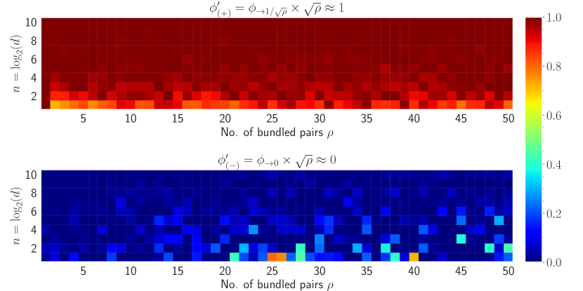
Figure 1: Empirical comparison of the corrected cosine similarity scores between $\phi^{\prime}_{(+)}$ (on top) and $\phi^{\prime}_{(-)}$ (on bottom) for varying $n$ and $\rho$ shown in heatmap. The dimension, i.e., $d=2^{n}$ is varied from $2$ to $1024$ $(n\in\{1,2,\cdots,10\})$ and the number of vector pairs bundled is varied from $1$ to $50$. This shows that we can accurately identify when a vector $\boldsymbol{x}$ has been bound to a VSA or not when we keep track of how many pairs of terms $\rho$ are included.

Empirical results of $\phi^{\prime}$ for varying $n$ and $\rho$ are visualized and verified by a heatmap. In a composite representation $\chi^{\prime}_{\rho}=\sum_{i=1}^{\rho}(x_{i}\odot y_{i})$, when unbinding is applied using the query $y_{i}$, i.e., ${\mathcal{B}^{*}}^{\prime}(\chi^{\prime}_{\rho},y_{i})=\hat{x_{i}}$, a positive case is a similarity between $x_{i}$ and $\hat{x_{i}}$. On the contrary, similarity between $\hat{x_{i}}$ and any $x_{j}$ where $j\in\{1,2,\cdots,\rho\}$ and $j\neq i$, is a negative case. Mean cosine similarity scores of $100$ trials for both positive and negative cases in presented in Figure 1 where the scores for the positive cases are in the red $(\approx 1)$ shades and the scores for the negative cases are in the blue $(\approx 0)$ shades.

4 Empirical Results

4.1 Classical VSA Tasks

A common VSA task is, given a bundle (addition) of $\rho$ pairs of bound vectors $\boldsymbol{s}=\sum_{i=1}^{\rho}\mathcal{B}(\boldsymbol{x}_{i},\boldsymbol{y}_{i})$, given a query $\boldsymbol{x}_{q}\in\boldsymbol{s}$, c can the corresponding vector $\boldsymbol{y}_{q}$ be correctly retrieved from the bundle. To test this, we perform an experiment similar to one in [38]. We first create a pool $P$ of $N=1000$ random vectors, then sample (with replacement) $p$ pairs of vectors for $p\in\{1,2,\cdots,25\}$. The pairs are bound together and added to create a composite representation $\boldsymbol{s}$. Then, we iterate through all left pairs $\boldsymbol{x}_{q}$ in the composite representation and attempt to retrieve the corresponding $\boldsymbol{y}_{q},\forall q\in[1,p]$. A retrieval is considered correct if $\mathcal{B}^{*}(\boldsymbol{s},\boldsymbol{x}_{q})^{\top}\boldsymbol{y}_{q}>\mathcal{B}^{*}(\boldsymbol{s},\boldsymbol{x}_{q})^{\top}\boldsymbol{y}_{j},\forall j\neq q$. The total accuracy score for the bundle is recorded, and the experiment is repeated for $50$ trials. Experiments are performed to compare HRR [33], VTB [13], MAP [11], and our HLB VSAs. For each VSA, at each dimension of the vector, the area under the curve (AUC) of the accuracy vs. the no. of bound terms plot is computed, and the results are shown in Figure 2. In general, HLB has comparable performance to HRR and VTB, and performs better than MAP.

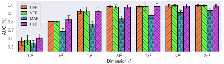
Figure 2: The area under the accuracy curve due to the change of no. of bundled pairs $\rho$ for dimensions $d$. All the dimensions are chosen to be perfect squares due to the constraint of VTB.

The scenario we just considered looked at bindings of only two items together, summed of many pairs of bindings. [13] proposed addition evaluations over sequential bindings that we now consider. In the random case we have an initial vector $\boldsymbol{b}_{0}$, and for $p$ rounds, we will modify it by a random vector $\boldsymbol{x}_{t}$ such that $\boldsymbol{b}_{t+1}=\mathcal{B}(\boldsymbol{b}_{t},\boldsymbol{x}_{t})$, after which we unbind each $\boldsymbol{x}_{t}$ to see how well the previous $\boldsymbol{b}_{t}$ is recovered. In the auto binding case, we use a single random vector $\boldsymbol{x}$ for all $p$ rounds.

In this task, we are concerned with the quality of the similarity score in random/auto-binding, as we want $\mathcal{B}^{*}(\boldsymbol{b}_{t+1},\boldsymbol{x}_{t})^{\top}\boldsymbol{b}_{t}=1$. For VSAs with approximate unbinding procedures, such as HRR, VTB, and MAP-C, the returned value will be 1 if $p=1$ but will decay as $p$ increases. HLBuses an exact unbinding procedure so that the returned value is expected to be 1 $\forall\ p$. We are also interested in the magnitude of the vectors $\|\mathcal{B}^{*}(\boldsymbol{b}_{t+1},\boldsymbol{x}_{t})\|_{2}$, where an ideal VSA has a constant magnitude that does not explode/vanish as $p$ increases.

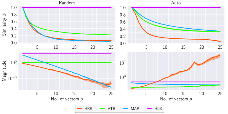
Figure 3: When repeatedly binding different random (left) or a single vector (right), HLB consistently returns the ideal similarity score of 1 for a present item (top row) and has a constant magnitude (bottom row), avoiding exploding/vanishing values.

Figure 3 shows that HLB maintains a stable magnitude regardless of the number of bound vectors in both cases. This property arises due to the properties of the distribution shown in 3.1. As all components have an expected absolute value of 1, the product of all components also has an expected absolute value of 1. Thus, the norm of the binding is simply $\sqrt{d}$. It also shows HLB maintains the desired similarity score as $p$ increases. Combined with Figure 1 that shows the scores are near-zero when an item is not present, HLB has significant advantages in consistency for designing VSA solutions.

4.2 Deep Learning with Hadamard-derived Linear Binding

Two recent methods that integrate HRR with deep learning are tested to further validate our approach and briefly summarized in the two sub-sections below. In each case, we run all four VSAs and see that HLB either matches or exceeds the performance of other VSAs. In every experiment, the standard method of sampling vectors from each VSA is followed as outlined in Table 1. All the experiments are performed on a single NVIDIA TESLA PH402 GPU with $32$GB memory.

4.2.1 Connectionist Symbolic Pseudo Secrets

When running on low-power computing environments, it is often desirable to offload the computation to a third-party cloud environment to get the answer faster and use fewer local resources. However, this may be problematic if one does not fully trust the available cloud environments. Homomorphic encryption (HE) is the ideal means to alleviate this problem, providing cryptography for computations. HE is currently more expensive to perform than running a neural network itself [12], defeating its own utility in this scenario. Connectionist Symbolic Pseudo Secrets (CSPS) [4] provides a heuristic means of obscuring the nature of the input (content), and output (number of classes/prediction), while also reducing the total local compute required.

CSPS mimics a “one-time-pad” by taking a random VSA vector $\boldsymbol{s}$ as the secret and binding it to the input $\boldsymbol{x}$. The value $\mathcal{B}(\boldsymbol{s},\boldsymbol{x})$ obscures the original $\boldsymbol{x}$, and the third-party runs the bulk of the network on their platform. A result $\boldsymbol{\tilde{y}}$ is returned, and a small local network computes the final answer after unbinding with the secret $\mathcal{B}^{*}(\boldsymbol{\tilde{y}},\boldsymbol{s})$. Other than changing the VSA used, we follow the same training, testing, architecture size, and validation procedure of [4].

CSPS experimented with 5 datasets MNIST, SVHN, CIFAR-10 (CR10), CIFAR-100 (CR100), and Mini-ImageNet (MIN). First, we look at the accuracy of each method, which is lower due to the noise of the random vector $\boldsymbol{s}$ added at test time since no secret VSA is ever reused. The results are shown in Table 2, where HLB outperforms all prior methods significantly. Notably, the MAP VSA is second best despite being one of the older VSAs, indicating its similarity to HLB in using a simple binding procedure, and thus simple gradient may be an important factor in this scenario.

Table 2: Accuracy comparison of the proposed HLB with HRR, VTB, MAP-C, and MAP-B in CSPS. The dimensions of the inputs along with the no. of classes are listed in the Dims/Labels column. The last row shows the geometric mean of the results.

Dataset	Dims/ Labels	CSPS + HRR		CSPS + VTB		CSPS + MAP-C		CSPS + MAP-B		CSPS + HLB
		Top@1	Top@5	Top@1	Top@5	Top@1	Top@5	Top@1	Top@5	Top@1	Top@5
MNIST	$28^{2}/10$	$98.51$	–	$98.44$	–	$98.46$	–	$98.40$	–	$\mathbf{98.73}$	–
SVHN	$32^{2}/10$	$88.44$	–	$19.59$	–	$79.95$	–	$92.43$	–	$\mathbf{94.53}$	–
CR10	$32^{2}/10$	$78.21$	–	$74.22$	–	$76.69$	–	$82.83$	–	$\mathbf{83.81}$	–
CR100	$32^{2}/100$	$48.84$	$75.82$	$35.87$	$61.79$	$56.77$	$81.52$	$57.76$	$84.63$	$\mathbf{58.82}$	$\mathbf{87.50}$
MIN	$84^{2}/100$	$40.99$	$66.99$	$45.81$	$73.52$	$52.22$	$78.63$	$57.91$	$82.81$	$\mathbf{59.48}$	$\mathbf{83.35}$
GM		$67.14$	$71.26$	$47.24$	$67.40$	$70.89$	$80.06$	$75.90$	$83.72$	$\mathbf{77.17}$	$\mathbf{85.40}$

Table 3: Clustering results of the main network inputs (top rows) and outputs (bottom rows) in terms of Adjusted Rand Index (ARI). Because CSPS is trying to hide information, scores near zero are better. Cell color corresponds to the cell absolute value, with blue indicating lower ARI and red indicating higher ARI. All numbers in percentages, and show HLB is better at information hiding.

Clustering Methods	HRR					VTB
	MNIST	SVHN	CR10	CR100	MIN	MNIST	SVHN	CR10	CR100	MIN
K-Means	$-0.02$	$-0.01$	$0.18$	$0.54$	$0.42$	$-0.00$	$-0.01$	$-0.01$	$0.02$	$0.00$
GMM	$0.01$	$0.00$	$0.09$	$0.61$	$0.44$	$4.67$	$1.37$	$-0.01$	$0.02$	$0.01$
Birch	$0.20$	$0.00$	$0.14$	$0.45$	$0.35$	$0.02$	$0.03$	$0.04$	$0.08$	$0.03$
HDBSCAN	$0.00$	$-0.24$	$1.23$	$0.01$	$0.02$	$0.00$	$0.00$	$0.00$	$0.00$	$0.00$
K-Means	$1.28$	$0.06$	$0.21$	$0.03$	$0.08$	$8.52$	$0.13$	$1.11$	$0.05$	$0.12$
GMM	$1.28$	$0.06$	$0.17$	$0.04$	$0.09$	$8.63$	$0.14$	$1.63$	$0.05$	$0.00$
Birch	$1.51$	$0.03$	$0.13$	$0.05$	$0.07$	$3.24$	$0.00$	$0.64$	$0.06$	$0.17$
HDBSCAN	$0.00$	$0.00$	$0.00$	$0.00$	$0.00$	$0.00$	$0.09$	$0.00$	$0.00$	$0.00$
Clustering Methods	MAP					HLB
	MNIST	SVHN	CR10	CR100	MIN	MNIST	SVHN	CR10	CR100	MIN
K-Means	$0.17$	$0.01$	$0.01$	$0.00$	$0.00$	$0.09$	$0.00$	$0.00$	$0.00$	$0.00$
GMM	$3.39$	$-0.01$	$0.01$	$0.00$	$0.00$	$2.53$	$0.00$	$0.00$	$0.00$	$0.00$
Birch	$0.84$	$-0.00$	$0.00$	$0.01$	$0.00$	$0.83$	$0.00$	$0.00$	$0.01$	$0.00$
HDBSCAN	$0.00$	$0.00$	$0.00$	$0.00$	$0.00$	$0.00$	$0.00$	$0.00$	$0.00$	$0.00$
K-Means	$15.91$	$0.09$	$0.00$	$0.03$	$0.01$	$13.67$	$-0.04$	$0.01$	$0.02$	$-0.00$
GMM	$42.43$	$0.11$	$0.00$	$0.03$	$0.00$	$14.96$	$-0.04$	$0.01$	$0.02$	$0.00$
Birch	$7.09$	$-0.07$	$-0.02$	$0.01$	$-0.00$	$18.44$	$-0.07$	$0.00$	$0.01$	$0.02$
HDBSCAN	$0.48$	$0.00$	$0.00$	$0.00$	$0.00$	$7.60$	$0.01$	$0.00$	$0.00$	$0.00$

However, improved accuracy is not useful in this scenario if more information is leaked. The test in this scenario, as proposed by  [4], is to calculate the Adjusted Rand Index (ARI) after attempting to cluster the inputs $\boldsymbol{x}$ and the outputs $\boldsymbol{\hat{y}}$, which are available/visible to the snooping third-party. To be successful, the ARI must be near zero (indicating random label assignment) for both inputs and outputs.

We use K-means, Gaussian Mixture Model (GMM), Birch [46], and HDBSCAN [8] as the clustering algorithms and specify the true number of classes to each method to maximize attacker success (information they would not know). The results can be found in Table 3, where the top rows indicate the clustering of the input $\mathcal{B}(\boldsymbol{x},\boldsymbol{s})$, and the bottom rows the clustering of the output $\boldsymbol{\hat{y}}$. All the numbers are percentages $(\%)$, showing all methods do a good job at hiding information from the adversary (except on the MNIST dataset, which is routinely degenerate).

The MNIST result is a good reminder that CSPS security is heuristic, not guaranteed. Nevertheless, we see HLB has consistently close-to-zero scores for SVHN, CIFARs, and Mini-ImageNet, indicating that its improved accuracy with simultaneously improved security. This also validates the use of the VSA in deep learning architecture design and the efficacy of our approach.

4.2.2 Xtreme Multi-Label Classification

Extreme Multi-label (XML) is the scenario where, given a single input of size $d$, $C>>d$ classes are used to predict. This is common in e-commerce applications where new products need to be tagged, and an input on the order of $d\approx 5000$ is relatively small compared to $C\geq$ 100,000 or more classes. This imposes unique computational constraints due to the output space being larger than the input space and is generally only solvable because the output space is sparse — often less than 100 relevant classes will be positive for any one input. VSAs have been applied to XML by exploiting the low positive class occurrence rate to represent the problem symbolically [10].

While many prior works focus on innovative strategies to cluster/make hierarchies/compress the penultimate layer[20, 21, 32, 19, 45, 23], a neuro-symbolic approach was proposed by [10]. Given $K$ total possible classes, they assigned each class a vector $\boldsymbol{c}_{k}$ to be each class’s representation, and the set of all classes $\boldsymbol{a}=\sum_{k=1}^{K}\boldsymbol{c}_{k}$.

The VSA trick used by [10] was to define an additional “present” class $\boldsymbol{p}$ and a “missing” class $\boldsymbol{m}$. Then, the target output of the network $f(\cdot)$ is itself a vector composed of two parts added together. First, $\mathcal{B}(\boldsymbol{p},\sum_{k}\boldsymbol{c}_{k})$ represents all present classes, and so the sum is over a finite smaller set. Then the absent classes compute the missing representing $\mathcal{B}(\boldsymbol{m},\boldsymbol{a}-\sum_{k}\boldsymbol{c}_{k})$, which again only needs to compute over the finite set of present classes, yet represents the set of all non-present classes by exploiting the symbolic properties of the VSA.

For XML classification, we have a set of $K$ classes that will be present for a given input, where $K\approx 10$ is the norm. Yet, there will be $L$ total possible classes where $L\geq 100,000$ is quite common. Forming a normal linear layer to produce $L$ outputs is the majority of computational work and memory use in standard XML models, and thus the target for reduction. A VSA can be used to side-step this cost, as shown by [10], by leveraging the symbolic manipulation of the outputs. First, consider the target label as a vector $\boldsymbol{s}\in\mathrm{R}^{d}$ such that $d\ll L$. By defining a VSA vector to represent “present” and “missing” classes as $\mathbf{p}$ and $\mathbf{m}$, where each class is given its own vector $\boldsymbol{c}_{1,\ldots,L}$, we can shift the computational complexity form $\mathcal{O}(L)$ to $\mathcal{O}(K)$ by manipulating the “missing” classes as the compliment of the present classes as shown in Equation 12.

Similarly, the loss to calculate the gradient can be computed based on the network’s prediction $\boldsymbol{\hat{s}}$ by taking the cosine similarity between each expected class and one cosine similarity for the representation of all missing classes. The excepted response of 1 or 0 for an item being present/absent from the VSA is used to determine if we want the similarity to be 0 (1-$\cos$) or 1 (just $\cos$), as shown in Equation 13.

$$\boldsymbol{s}=\overbrace{\sum_{i\in y_{i}=1}\mathcal{B}(\boldsymbol{p},\boldsymbol{c}_{i})}^{\text{Labels Present}\mathcal{O}(dK)}+\overbrace{\sum_{j\in y_{j}=-1}\mathcal{B}(\boldsymbol{m},\boldsymbol{c}_{j})}^{\text{Labels Absent}\mathcal{O}(dL)}=\overbrace{\mathcal{B}\left(\boldsymbol{p},\left(\boldsymbol{a}\eqcolon\sum_{i\in y_{i}=1}c_{i}\right)\right)}^{\text{Labels Present}\mathcal{O}(d\ K)}+\overbrace{\mathcal{B}\left(\boldsymbol{m},\left(\boldsymbol{a}-\sum_{i\in y_{i}=1}c_{i}\right)\right)}^{\text{Labels Absent}\mathcal{O}(dK)}$$ (12)

$$loss=\ \overbrace{\sum_{i\in y_{i}=1}\left(1-\cos\left(\mathcal{B}^{*}(\boldsymbol{p},\hat{\boldsymbol{s}}),\boldsymbol{c}_{i}\right)\right)}^{\text{Present Classes}\ \mathcal{O}(d\ K)}+\overbrace{\cos\left(\mathcal{B}^{*}(\boldsymbol{m},\hat{s}),\sum_{i\in y_{i}=1}\boldsymbol{c}_{i}\ \right)}^{\text{Absent classes}\ O(d\ K)}$$ (13)

The details and network sizes of [10] are followed, except we replace the original VSA with our four candidates. The network is trained on $8$ datasets listed in Table 4 from [5] and evaluated using normalized discounted cumulative gain (nDCG) and propensity-scored (PS) based normalized discounted cumulative gain (PSnDCG) as suggested by [20].

Table 4: XML classification results in dense label representation with HRR, VTB, MAP, and HLB in terms of nDCG and PSnDCG. The proposed HLB has attained the best nDCG and PSnDCG scores on all the datasets setting a new SOTA.

Dataset	Bibtex		Delicious		Mediamill		EURLex-4K
Metrics	nDCG	PSnDCG	nDCG	PSnDCG	nDCG	PSnDCG	nDCG	PSnDCG
HRR	$60.296$	$45.572$	$66.454$	$30.016$	$83.885$	$63.684$	$77.225$	$30.684$
VTB	$57.693$	$45.219$	$63.325$	$31.449$	$87.232$	$66.948$	$76.964$	$31.180$
MAP-C	$59.280$	$46.092$	$65.376$	$31.943$	$87.255$	$66.886$	$72.439$	$26.752$
MAP-B	$59.412$	$46.340$	$65.431$	$32.122$	$86.886$	$66.562$	$71.128$	$26.340$
HLB	$\mathbf{61.741}$	$\mathbf{48.639}$	$\mathbf{67.821}$	$\mathbf{32.797}$	$\mathbf{88.064}$	$\mathbf{67.525}$	$\mathbf{77.868}$	$\mathbf{31.526}$
Dataset	EURLex-4.3K		Wiki10-31K		Amazon-13K		Delicious-200K
Metrics	nDCG	PSnDCG	nDCG	PSnDCG	nDCG	PSnDCG	nDCG	PSnDCG
HRR	$84.497$	$38.545$	$81.068$	$9.185$	$93.258$	$49.642$	$44.933$	$6.839$
VTB	$84.663$	$38.540$	$78.025$	$9.645$	$92.373$	$49.463$	$44.092$	$6.664$
MAP-C	$85.472$	$39.233$	$80.203$	$10.027$	$92.013$	$48.686$	$45.373$	$6.862$
MAP-B	$85.023$	$38.820$	$80.238$	$10.035$	$92.307$	$48.812$	$45.459$	$6.870$
HLB	$\mathbf{88.204}$	$\mathbf{43.622}$	$\mathbf{83.589}$	$\mathbf{11.869}$	$\mathbf{93.672}$	$\mathbf{50.270}$	$\mathbf{46.331}$	$\mathbf{6.952}$

The classification result in terms of nDCG and PSnDCG in all the eight datasets is presented in Table 4 where the top four datasets are comparatively easy with maximum no. of features of $5000$ and no. of labels of $4000$. The bottom four datasets are comparatively hard with the no. of features and labels on the scale of $100K$. The proposed HLB has attained the best results in all the datasets on both metrics. In contrast to the prior CSPS results, here we see that the performance differences between HRR, VTB, and MAP are more varied, with no clear “second-place” performer.

5 Conclusion

In this paper, a novel linear vector symbolic architecture named HLB is presented derived from Hadamard transform. Along with an initialization condition named MiND distribution is proposed for which we proved the cosine similarity $\phi$ is approximately equal to the inverse square root of the no. of bundled vector pairs $\rho$ which matches with the experimental results. The proposed HLB showed superior performance in classical VSA tasks and deep learning compared to other VSAs such as HRR, VTB, and MAP. In learning tasks, HLB is applied to CSPS and XML classification tasks. In both of the tasks, HLB has achieved the best results in terms of respective metrics in all the datasets showing a diverse potential of HLB in Neuro-symbolic AI.

Appendix A Noise Decomposition

When a single vector pair is combined, one of the vector pairs can be exactly retrieved with the help of the other component and the inverse function, recalling the retrieved output does not contain any noise component for a single pair of vectors, i.e., $\rho=1$. However, when more than one vector pairs are bundled, noise starts to accumulate. In this section, we will uncover the noise components accumulated with and without the projection to the inputs and analyze their impact on expectation. We first start with the noise component without the projection step $\eta_{i}^{\circ}$.

$$\eta_{i}^{\circ}=\frac{1}{d}\cdot H(\frac{1}{Hy_{i}}\odot\sum_{\begin{subarray}{c}j=1\\ j\neq i\end{subarray}}^{\rho}(Hx_{j}\odot Hy_{j})$$ (14)

Let, set the value of $n$ to be $1$ thus, $d=2^{n}=2$ and the number of vector pairs $\rho=2$, i.e., $\chi_{\rho=2}=\mathcal{B}(x_{1},y_{1})+\mathcal{B}(x_{2},y_{2})$. We want to retrieve $x_{1}$ using the query $y_{1}$, thereby, the expression of $\eta_{i}^{\circ}$ is uncovered step by step for $\rho=2$ shown in Equation 15.

$$\begin{split}\underset{\rho=2}{\eta_{i}^{\circ}}&=\frac{1}{d}\cdot H(\frac{1}{Hy_{1}}\odot(Hx_{2}\odot Hy_{2}))\\ &=\frac{1}{d}\cdot\sqrt{d}\cdot H\left(\begin{array}[]{c}\frac{1}{y_{1}^{(0)}+y_{1}^{(1)}}\\ \frac{1}{y_{1}^{(0)}-y_{1}^{(1)}}\end{array}\odot\begin{array}[]{cc}(x_{2}^{(0)}+x_{2}^{(1)})\cdot(y_{2}^{(0)}+y_{2}^{(1)})\\ (x_{2}^{(0)}-x_{2}^{(1)})\cdot(y_{2}^{(0)}-y_{2}^{(1)})\end{array}\right)\\ &=\frac{1}{d}\cdot d\cdot\left(\begin{array}[]{c}\frac{(x_{2}^{(0)}+x_{2}^{(1)})\,(y_{2}^{(0)}+y_{2}^{(1)})\,(y_{1}^{(0)}-y_{1}^{(1)})\,+\,(x_{2}^{(0)}-x_{2}^{(1)})\,(y_{2}^{(0)}-y_{2}^{(1)})\,(y_{1}^{(0)}+y_{1}^{(1)})}{(y_{1}^{(0)}+y_{1}^{(1)})\,(y_{1}^{(0)}-y_{1}^{(1)})}\\ \frac{(x_{2}^{(0)}+x_{2}^{(1)})\,(y_{2}^{(0)}+y_{2}^{(1)})\,(y_{1}^{(0)}-y_{1}^{(1)})\,-\,(x_{2}^{(0)}-x_{2}^{(1)})\,(y_{2}^{(0)}-y_{2}^{(1)})\,(y_{1}^{(0)}+y_{1}^{(1)})}{(y_{1}^{(0)}+y_{1}^{(1)})\,(y_{1}^{(0)}-y_{1}^{(1)})}\end{array}\right)\\ &=\left(\begin{array}[]{c}\frac{\varphi_{1}}{\prod_{k=1}^{d}(Hy_{1})_{k}}\\ \frac{\varphi_{2}}{\prod_{k=1}^{d}(Hy_{1})_{k}}\end{array}\right)\\ &=\frac{\mathcal{P}(x_{2},y_{2},y_{1})}{\prod_{k=1}^{d}(Hy_{1})_{k}}\end{split}$$ (15)

Here, $\varphi_{k}\;\forall\;k\in\mathbb{N}:1\leq k\leq d$ are the polynomials comprises of $(x_{2},~{}y_{2})$, and the query vector $y_{1}$. $\mathcal{P}$ is the vector of polynomials consisting of $\varphi_{k}$. From the noise expression, we can observe that the numerator is a polynomial and the denominator is the product of all the elements of the Hadamard transformation of the query vector. This is true for any value of $n$ and $\rho$. Thus, in general, for any query $y_{i}$ we can express $\eta_{i}^{\circ}$ as shown in Equation 16.

$$\eta_{i}^{\circ}=\frac{\operatorname*{\mathcal{P}}\limits_{\begin{subarray}{c}j=1,~{}j\neq i\end{subarray}}^{\rho}{(x_{j},y_{j},y_{i})}}{\prod_{k=1}^{d}(Hy_{i})_{k}}$$ (16)

The noise accumulated after applying the projection to the inputs is quite straightforward as given in Equation 17.

$$\eta_{i}^{\pi}=\frac{\sum\limits_{\begin{subarray}{c}j=1,~{}j\neq i\end{subarray}}^{\rho}(x_{j}\odot y_{j})}{y_{i}}$$ (17)

Although the vectors $x_{i},y_{i}\;\forall\;i\in\mathbb{N}:1\leq i\leq\rho$ are sampled from a MiND with an expected value of $0$ given in Equation 7, the sample mean of $x_{i}$ or $y_{i}$ would be $\hat{\mu}\approx 0$ but $\hat{\mu}\neq 0$. Both the numerator of $\eta_{i}^{\circ}$ and $\eta_{i}^{\pi}$ are the polynomials thus the expected value would be very close to $0$. However, the expected value of the denominator of $\eta_{i}^{\circ}$ would be $\mathrm{E}[\prod_{k=1}^{d}(Hy_{i})_{k}]=\prod_{k=1}^{d}\mathrm{E}[(Hy_{i})_{k}]={\hat{\mu}}^{d}$ whereas the expected value of the denominator of $\eta_{i}^{\pi}$ is $\mathrm{E}[y_{i}]=\hat{\mu}$. Since, $\hat{\mu}^{d}<\hat{\mu}$, hence, in expectation $\eta_{i}^{\pi}<\eta_{i}^{\circ}$. This is also verified by an empirical study where $n$, i.e., the dimension $d=2^{n}$ is varied along with the no. of bound vector pairs $\rho$ and the amount of absolute mean noise in retrieval is estimated.

Figure 4 shows the heatmap visualization of the noise for both $\eta_{i}^{\circ}$ and $\eta_{i}^{\pi}$ in natural log scale. The amount of noise accumulated without any projection to the inputs is much higher compared to the noise accumulation with the projection. For varying $n$ and $\rho$, the maximum amount of noise accumulated when projection is applied is $7.18$ and without any projection, the maximum amount of noise is $19.38$. Also, most of the heatmap of $\eta_{i}^{\pi}$ remains in the blue region whereas as $n$ and $\rho$ increase, the heatmap of $\eta_{i}^{\circ}$ moves towards the red region. Therefore, it is evident that the projection to the inputs diminishes the amount of accumulated noise with the retrieved output.

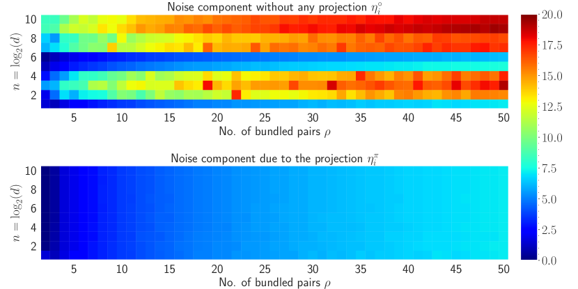
Figure 4: Heatmap of the empirical comparison of the noise components $\eta_{i}^{\circ}$ and $\eta_{i}^{\pi}$ for varying $n$ and $\rho$ shown in natural logarithm scale. The dimension, i.e., $d=2^{n}$ is varied from $2$ to $1024$ $(n\in\{1,2,\cdots,10\})$ and the number of vector pairs bundled is varied from $2$ to $50$.

Appendix B Norm Relation

Theorem B.1 ($\chi_{\rho}$ – $\rho$ Relationship).

Given $x_{i},y_{i}\sim\Omega(\mu,1/d)\in\mathbb{R}^{d}\;\forall\;i\in\mathbb{N}:1\leq i\leq\rho$, the norm of the composite representation $\chi_{\rho}$ is proportional to $\sqrt{\rho}$ and approximately equal to the $\mu^{2}\sqrt{\rho\cdot d}$.

Proof of Theorem B.1.

Given $\chi_{\rho}$ is the composite representation of the bound vectors, i.e., the summation of $\rho$ no. of individual bound terms. First, let’s compute the norm of the single bound term as shown in Equation 18.

$$\begin{split}\left\|\mathcal{B}(x_{i},y_{i})\right\|_{2}&=\left\|x_{i}\cdot y_{i}\right\|_{2}\\ &=\sqrt{(x_{i}^{(1)}y_{i}^{(1)})^{2}+(x_{i}^{(2)}y_{i}^{(2)})^{2}+\cdots+(x_{i}^{(d)}y_{i}^{(d)})^{2}}\\ &=\sqrt{(\pm\mu^{2})^{2}+(\pm\mu^{2})^{2}+\cdots+(\pm\mu^{2})^{2}}\quad\left[E[x^{(1)}]\cdot E[y^{(1)}]=\pm\mu\cdot\pm\mu=\pm\mu^{2}\right]\\ &=\sqrt{\mu^{4}d}\end{split}$$ (18)

Now, let’s expand and compute the square norm of the composite representation given in Equation 19.

$$\begin{split}\left\|\chi_{\rho}\right\|^{2}_{2}&=\left\|\mathcal{B}(x_{1},y_{1})+\mathcal{B}(x_{2},y_{2})+\cdots+\mathcal{B}(x_{\rho},y_{\rho})\right\|^{2}_{2}\\ &=\left\|\mathcal{B}(x_{1},y_{1})\right\|^{2}_{2}+\left\|\mathcal{B}(x_{2},y_{2})\right\|^{2}_{2}+\cdots+\left\|\mathcal{B}(x_{\rho},y_{\rho})\right\|^{2}_{2}\;+\;\xi\\ &\text{where $\xi$ is the rest of the terms of square expansion.}\\ &=\mu^{4}d+\mu^{4}d+\cdots+\mu^{4}d+\xi\\ &=\rho\cdot\mu^{4}d+\xi\\ \left\|\chi_{\rho}\right\|_{2}&=\sqrt{\rho\cdot\mu^{4}d+\xi}\\ &\approx\sqrt{\rho\cdot\mu^{4}d}\quad\left[\text{ $\xi$ is the noise term and discarded to make an approximation }\right]\\ &=\mu^{2}\sqrt{\rho\cdot d}\qed\end{split}$$ (19)

Thus, given the composite representation and the mean of the MiND distribution, we can estimate the no. of bound terms bundled together by $\rho\approx\left\|\chi_{\rho}\right\|^{2}_{2}/\mu^{4}d$. ∎

Figure 5 shows the comparison between the theoretical relationship and actual experimental results where the norm of the composite representation is computed for $\mu=0.5$ and $\rho=\{1,2,\cdots,200\}$. The figure indicates that the theoretical relationship aligns with the experimental results. However, as the number of bundled pair increases, the variation in the norm increases. This is because of making the approximation by discarding $\xi$ in Equation 19.

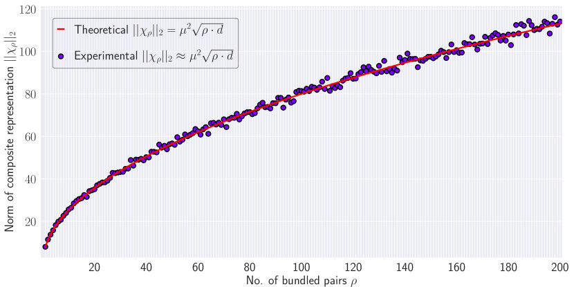
Figure 5: Comparison between the theoretical and experimental relationship of Theorem B.1. The norm of the composite representation of the bound vectors is computed for no. of bundled vectors from $1$ to $200$ of dimension $d=1024$. The figure shows how the experimental value of the norm closely follows the theoretical relation between $\left\|\chi_{\rho}\right\|_{2}$ and $\rho$.

Appendix C Cosine Relation

Theorem 3.2 shows how the cosine similarity $\phi$ between the original $x_{i}$ and retrieved vector $\hat{x_{i}}$ is approximately equal to the inverse square root of the number of vector pairs in a composite representation $\rho$. In this section, we will perform an empirical analysis of the theorem and compare it with the theoretical results. For $\rho=\{1,2,\cdots,50\}$, similarity score $\phi$ is calculated for vector dimension $d=512$. Additionally, the theoretical cosine similarity score is also calculated using the value of $\phi$ following the theorem. Figure 6 shows the comparison between the two results where the experimental result closely follows the theoretical result. The figure also shows the standard deviation for $100$ trials, indicating a minute change from the actual value.

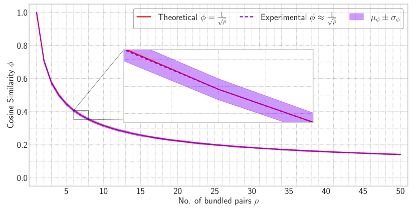
Figure 6: Comparison between the theoretical and experimental $\phi-\rho$ relationship. Vectors of dimension $d=512$ are combined and retrieved with a varied number of vectors from $1$ to $50$. The zoom portion shows how closely experimental results match with the theoretical conclusion.

NeurIPS Paper Checklist

1. Claims

2. Question: Do the main claims made in the abstract and introduction accurately reflect the paper’s contributions and scope?

3. Answer: [Yes]

4. Justification: The paper claims to present a new Hadamard-derived linear vector symbolic architecture in the abstract and introduction which accurately reflects the contribution and scope of the paper.

5. Guidelines:

   • The answer NA means that the abstract and introduction do not include the claims made in the paper.

   • The abstract and/or introduction should clearly state the claims made, including the contributions made in the paper and important assumptions and limitations. A No or NA answer to this question will not be perceived well by the reviewers.

   • The claims made should match theoretical and experimental results, and reflect how much the results can be expected to generalize to other settings.

   • It is fine to include aspirational goals as motivation as long as it is clear that these goals are not attained by the paper.

6. Limitations

7. Question: Does the paper discuss the limitations of the work performed by the authors?

8. Answer: [Yes]

9. Justification: Limitations are described in the paper.

10. Guidelines:

    • The answer NA means that the paper has no limitation while the answer No means that the paper has limitations, but those are not discussed in the paper.

    • The authors are encouraged to create a separate "Limitations" section in their paper.

    • The paper should point out any strong assumptions and how robust the results are to violations of these assumptions (e.g., independence assumptions, noiseless settings, model well-specification, asymptotic approximations only holding locally). The authors should reflect on how these assumptions might be violated in practice and what the implications would be.

    • The authors should reflect on the scope of the claims made, e.g., if the approach was only tested on a few datasets or with a few runs. In general, empirical results often depend on implicit assumptions, which should be articulated.

    • The authors should reflect on the factors that influence the performance of the approach. For example, a facial recognition algorithm may perform poorly when image resolution is low or images are taken in low lighting. Or a speech-to-text system might not be used reliably to provide closed captions for online lectures because it fails to handle technical jargon.

    • The authors should discuss the computational efficiency of the proposed algorithms and how they scale with dataset size.

    • If applicable, the authors should discuss possible limitations of their approach to address problems of privacy and fairness.

    • While the authors might fear that complete honesty about limitations might be used by reviewers as grounds for rejection, a worse outcome might be that reviewers discover limitations that aren’t acknowledged in the paper. The authors should use their best judgment and recognize that individual actions in favor of transparency play an important role in developing norms that preserve the integrity of the community. Reviewers will be specifically instructed to not penalize honesty concerning limitations.

11. Theory Assumptions and Proofs

12. Question: For each theoretical result, does the paper provide the full set of assumptions and a complete (and correct) proof?

13. Answer: [Yes]

14. Justification: All the theoretical results and proofs are provided in the Methodology section. (See section 3)

15. Guidelines:

    • The answer NA means that the paper does not include theoretical results.

    • All the theorems, formulas, and proofs in the paper should be numbered and cross-referenced.

    • All assumptions should be clearly stated or referenced in the statement of any theorems.

    • The proofs can either appear in the main paper or the supplemental material, but if they appear in the supplemental material, the authors are encouraged to provide a short proof sketch to provide intuition.

    • Inversely, any informal proof provided in the core of the paper should be complemented by formal proofs provided in appendix or supplemental material.

    • Theorems and Lemmas that the proof relies upon should be properly referenced.

16. Experimental Result Reproducibility

17. Question: Does the paper fully disclose all the information needed to reproduce the main experimental results of the paper to the extent that it affects the main claims and/or conclusions of the paper (regardless of whether the code and data are provided or not)?

18. Answer: [Yes]

19. Justification: The experimental setup is based on previous papers. All the self-used parameters are discussed in the paper.

20. Guidelines:

    • The answer NA means that the paper does not include experiments.

    • If the paper includes experiments, a No answer to this question will not be perceived well by the reviewers: Making the paper reproducible is important, regardless of whether the code and data are provided or not.

    • If the contribution is a dataset and/or model, the authors should describe the steps taken to make their results reproducible or verifiable.

    • Depending on the contribution, reproducibility can be accomplished in various ways. For example, if the contribution is a novel architecture, describing the architecture fully might suffice, or if the contribution is a specific model and empirical evaluation, it may be necessary to either make it possible for others to replicate the model with the same dataset, or provide access to the model. In general. releasing code and data is often one good way to accomplish this, but reproducibility can also be provided via detailed instructions for how to replicate the results, access to a hosted model (e.g., in the case of a large language model), releasing of a model checkpoint, or other means that are appropriate to the research performed.

    • While NeurIPS does not require releasing code, the conference does require all submissions to provide some reasonable avenue for reproducibility, which may depend on the nature of the contribution. For example

      1. If the contribution is primarily a new algorithm, the paper should make it clear how to reproduce that algorithm.

      2. If the contribution is primarily a new model architecture, the paper should describe the architecture clearly and fully.

      3. If the contribution is a new model (e.g., a large language model), then there should either be a way to access this model for reproducing the results or a way to reproduce the model (e.g., with an open-source dataset or instructions for how to construct the dataset).

      4. We recognize that reproducibility may be tricky in some cases, in which case authors are welcome to describe the particular way they provide for reproducibility. In the case of closed-source models, it may be that access to the model is limited in some way (e.g., to registered users), but it should be possible for other researchers to have some path to reproducing or verifying the results.

21. Open access to data and code

22. Question: Does the paper provide open access to the data and code, with sufficient instructions to faithfully reproduce the main experimental results, as described in supplemental material?

23. Answer: [Yes]

24. Justification: All the code is provided with the supplemental material. Data is publicly available and instruction is provided on how to get the data.

25. Guidelines:

    • The answer NA means that paper does not include experiments requiring code.

    • Please see the NeurIPS code and data submission guidelines (https://nips.cc/public/guides/CodeSubmissionPolicy) for more details.

    • While we encourage the release of code and data, we understand that this might not be possible, so “No” is an acceptable answer. Papers cannot be rejected simply for not including code, unless this is central to the contribution (e.g., for a new open-source benchmark).

    • The instructions should contain the exact command and environment needed to run to reproduce the results. See the NeurIPS code and data submission guidelines (https://nips.cc/public/guides/CodeSubmissionPolicy) for more details.

    • The authors should provide instructions on data access and preparation, including how to access the raw data, preprocessed data, intermediate data, and generated data, etc.

    • The authors should provide scripts to reproduce all experimental results for the new proposed method and baselines. If only a subset of experiments are reproducible, they should state which ones are omitted from the script and why.

    • At submission time, to preserve anonymity, the authors should release anonymized versions (if applicable).

    • Providing as much information as possible in supplemental material (appended to the paper) is recommended, but including URLs to data and code is permitted.

26. Experimental Setting/Details

27. Question: Does the paper specify all the training and test details (e.g., data splits, hyperparameters, how they were chosen, type of optimizer, etc.) necessary to understand the results?

28. Answer: [Yes]

29. Justification: Experimental details and their sources are cited in the Empirical results section. (see section 4)

30. Guidelines:

    • The answer NA means that the paper does not include experiments.

    • The experimental setting should be presented in the core of the paper to a level of detail that is necessary to appreciate the results and make sense of them.

    • The full details can be provided either with the code, in appendix, or as supplemental material.

31. Experiment Statistical Significance

32. Question: Does the paper report error bars suitably and correctly defined or other appropriate information about the statistical significance of the experiments?

33. Answer: [Yes]

34. Justification: See Figure 2, Figure 3

35. Guidelines:

    • The answer NA means that the paper does not include experiments.

    • The authors should answer "Yes" if the results are accompanied by error bars, confidence intervals, or statistical significance tests, at least for the experiments that support the main claims of the paper.

    • The factors of variability that the error bars are capturing should be clearly stated (for example, train/test split, initialization, random drawing of some parameter, or overall run with given experimental conditions).

    • The method for calculating the error bars should be explained (closed form formula, call to a library function, bootstrap, etc.)

    • The assumptions made should be given (e.g., Normally distributed errors).

    • It should be clear whether the error bar is the standard deviation or the standard error of the mean.

    • It is OK to report 1-sigma error bars, but one should state it. The authors should preferably report a 2-sigma error bar than state that they have a 96% CI, if the hypothesis of Normality of errors is not verified.

    • For asymmetric distributions, the authors should be careful not to show in tables or figures symmetric error bars that would yield results that are out of range (e.g. negative error rates).

    • If error bars are reported in tables or plots, The authors should explain in the text how they were calculated and reference the corresponding figures or tables in the text.

36. Experiments Compute Resources

37. Question: For each experiment, does the paper provide sufficient information on the computer resources (type of compute workers, memory, time of execution) needed to reproduce the experiments?

38. Answer: [Yes]

39. Justification: See section 4.

40. Guidelines:

    • The answer NA means that the paper does not include experiments.

    • The paper should indicate the type of compute workers CPU or GPU, internal cluster, or cloud provider, including relevant memory and storage.

    • The paper should provide the amount of compute required for each of the individual experimental runs as well as estimate the total compute.

    • The paper should disclose whether the full research project required more compute than the experiments reported in the paper (e.g., preliminary or failed experiments that didn’t make it into the paper).

41. Code Of Ethics

42. Question: Does the research conducted in the paper conform, in every respect, with the NeurIPS Code of Ethics https://neurips.cc/public/EthicsGuidelines?

43. Answer: [Yes]

44. Justification: We followed the NeurIPS code of conduct.

45. Guidelines:

    • The answer NA means that the authors have not reviewed the NeurIPS Code of Ethics.

    • If the authors answer No, they should explain the special circumstances that require a deviation from the Code of Ethics.

    • The authors should make sure to preserve anonymity (e.g., if there is a special consideration due to laws or regulations in their jurisdiction).

46. Broader Impacts

47. Question: Does the paper discuss both potential positive societal impacts and negative societal impacts of the work performed?

48. Answer: [N/A]

49. Justification: The work has no negative societal impacts.

50. Guidelines:

    • The answer NA means that there is no societal impact of the work performed.

    • If the authors answer NA or No, they should explain why their work has no societal impact or why the paper does not address societal impact.

    • Examples of negative societal impacts include potential malicious or unintended uses (e.g., disinformation, generating fake profiles, surveillance), fairness considerations (e.g., deployment of technologies that could make decisions that unfairly impact specific groups), privacy considerations, and security considerations.

    • The conference expects that many papers will be foundational research and not tied to particular applications, let alone deployments. However, if there is a direct path to any negative applications, the authors should point it out. For example, it is legitimate to point out that an improvement in the quality of generative models could be used to generate deepfakes for disinformation. On the other hand, it is not needed to point out that a generic algorithm for optimizing neural networks could enable people to train models that generate Deepfakes faster.

    • The authors should consider possible harms that could arise when the technology is being used as intended and functioning correctly, harms that could arise when the technology is being used as intended but gives incorrect results, and harms following from (intentional or unintentional) misuse of the technology.

    • If there are negative societal impacts, the authors could also discuss possible mitigation strategies (e.g., gated release of models, providing defenses in addition to attacks, mechanisms for monitoring misuse, mechanisms to monitor how a system learns from feedback over time, improving the efficiency and accessibility of ML).

51. Safeguards

52. Question: Does the paper describe safeguards that have been put in place for responsible release of data or models that have a high risk for misuse (e.g., pretrained language models, image generators, or scraped datasets)?

53. Answer: [N/A]

54. Justification: No high-risk data or models are used.

55. Guidelines:

    • The answer NA means that the paper poses no such risks.

    • Released models that have a high risk for misuse or dual-use should be released with necessary safeguards to allow for controlled use of the model, for example by requiring that users adhere to usage guidelines or restrictions to access the model or implementing safety filters.

    • Datasets that have been scraped from the Internet could pose safety risks. The authors should describe how they avoided releasing unsafe images.

    • We recognize that providing effective safeguards is challenging, and many papers do not require this, but we encourage authors to take this into account and make a best faith effort.

56. Licenses for existing assets

57. Question: Are the creators or original owners of assets (e.g., code, data, models), used in the paper, properly credited and are the license and terms of use explicitly mentioned and properly respected?

58. Answer: [Yes]

59. Justification: Original paper and code are cited in the paper.

60. Guidelines:

    • The answer NA means that the paper does not use existing assets.

    • The authors should cite the original paper that produced the code package or dataset.

    • The authors should state which version of the asset is used and, if possible, include a URL.

    • The name of the license (e.g., CC-BY 4.0) should be included for each asset.

    • For scraped data from a particular source (e.g., website), the copyright and terms of service of that source should be provided.

    • If assets are released, the license, copyright information, and terms of use in the package should be provided. For popular datasets, paperswithcode.com/datasets has curated licenses for some datasets. Their licensing guide can help determine the license of a dataset.

    • For existing datasets that are re-packaged, both the original license and the license of the derived asset (if it has changed) should be provided.

    • If this information is not available online, the authors are encouraged to reach out to the asset’s creators.

61. New Assets

62. Question: Are new assets introduced in the paper well documented and is the documentation provided alongside the assets?

63. Answer: [Yes]

64. Justification: Documentation of the code is provided.

65. Guidelines:

    • The answer NA means that the paper does not release new assets.

    • Researchers should communicate the details of the dataset/code/model as part of their submissions via structured templates. This includes details about training, license, limitations, etc.

    • The paper should discuss whether and how consent was obtained from people whose asset is used.

    • At submission time, remember to anonymize your assets (if applicable). You can either create an anonymized URL or include an anonymized zip file.

66. Crowdsourcing and Research with Human Subjects

67. Question: For crowdsourcing experiments and research with human subjects, does the paper include the full text of instructions given to participants and screenshots, if applicable, as well as details about compensation (if any)?

68. Answer: [N/A]

69. Justification: No Crowdsourcing and Research with Human Subjects are used.

70. Guidelines:

    • The answer NA means that the paper does not involve crowdsourcing nor research with human subjects.

    • Including this information in the supplemental material is fine, but if the main contribution of the paper involves human subjects, then as much detail as possible should be included in the main paper.

    • According to the NeurIPS Code of Ethics, workers involved in data collection, curation, or other labor should be paid at least the minimum wage in the country of the data collector.

71. Institutional Review Board (IRB) Approvals or Equivalent for Research with Human Subjects

72. Question: Does the paper describe potential risks incurred by study participants, whether such risks were disclosed to the subjects, and whether Institutional Review Board (IRB) approvals (or an equivalent approval/review based on the requirements of your country or institution) were obtained?

73. Answer: [N/A]

74. Justification: No participants are used.

75. Guidelines:

    • The answer NA means that the paper does not involve crowdsourcing nor research with human subjects.

    • Depending on the country in which research is conducted, IRB approval (or equivalent) may be required for any human subjects research. If you obtained IRB approval, you should clearly state this in the paper.

    • We recognize that the procedures for this may vary significantly between institutions and locations, and we expect authors to adhere to the NeurIPS Code of Ethics and the guidelines for their institution.

    • For initial submissions, do not include any information that would break anonymity (if applicable), such as the institution conducting the review.

References

- [1]
- Alam et al. [2023b] Mohammad Mahmudul Alam, Edward Raff, Stella Biderman, Tim Oates, and James Holt. 2023b. Recasting self-attention with holographic reduced representations. In Proceedings of the 40th International Conference on Machine Learning (, Honolulu, Hawaii, USA,) (ICML’23). JMLR.org, Article 23, 18 pages.
- Alam et al. [2023a] Mohammad Mahmudul Alam, Edward Raff, and Tim Oates. 2023a. Towards Generalization in Subitizing with Neuro-Symbolic Loss using Holographic Reduced Representations. Neuro-Symbolic Learning and Reasoning in the era of Large Language Models (2023). https://doi.org/10.48550/arXiv.2312.15310
- Alam et al. [2022] Mohammad Mahmudul Alam, Edward Raff, Tim Oates, and James Holt. 2022. Deploying Convolutional Networks on Untrusted Platforms Using 2D Holographic Reduced Representations. In Proceedings of the 39th International Conference on Machine Learning (Proceedings of Machine Learning Research, Vol. 162), Kamalika Chaudhuri, Stefanie Jegelka, Le Song, Csaba Szepesvari, Gang Niu, and Sivan Sabato (Eds.). PMLR, 367–393. https://proceedings.mlr.press/v162/alam22a.html
- Bhatia et al. [2016] K. Bhatia, K. Dahiya, H. Jain, P. Kar, A. Mittal, Y. Prabhu, and M. Varma. 2016. The extreme classification repository: Multi-label datasets and code. http://manikvarma.org/downloads/XC/XMLRepository.html
- Blouw and Eliasmith [2013] Peter Blouw and Chris Eliasmith. 2013. A Neurally Plausible Encoding of Word Order Information into a Semantic Vector Space. 35th Annual Conference of the Cognitive Science Society 35 (2013), 1905–1910.
- Blouw et al. [2016] Peter Blouw, Eugene Solodkin, Paul Thagard, and Chris Eliasmith. 2016. Concepts as Semantic Pointers: A Framework and Computational Model. Cognitive Science 40, 5 (7 2016), 1128–1162. https://doi.org/10.1111/cogs.12265
- Campello et al. [2013] Ricardo JGB Campello, Davoud Moulavi, and Jörg Sander. 2013. Density-based clustering based on hierarchical density estimates. In Pacific-Asia conference on knowledge discovery and data mining. Springer, 160–172.
- Eliasmith et al. [2012] C. Eliasmith, T. C. Stewart, X. Choo, T. Bekolay, T. DeWolf, Y. Tang, and D. Rasmussen. 2012. A Large-Scale Model of the Functioning Brain. Science 338, 6111 (11 2012), 1202–1205. https://doi.org/10.1126/science.1225266
- Ganesan et al. [2021] Ashwinkumar Ganesan, Hang Gao, Sunil Gandhi, Edward Raff, Tim Oates, James Holt, and Mark McLean. 2021. Learning with holographic reduced representations. Advances in neural information processing systems 34 (2021), 25606–25620.
- Gayler [1998] Ross W. Gayler. 1998. Multiplicative Binding, Representation Operators & Analogy (Workshop Poster). http://cogprints.org/502/
- Gilad-Bachrach et al. [2016] Ran Gilad-Bachrach, Nathan Dowlin, Kim Laine, Kristin Lauter, Michael Naehrig, and John Wernsing. 2016. Cryptonets: Applying neural networks to encrypted data with high throughput and accuracy. In International conference on machine learning. PMLR, 201–210.
- Gosmann and Eliasmith [2019] Jan Gosmann and Chris Eliasmith. 2019. Vector-Derived Transformation Binding: An Improved Binding Operation for Deep Symbol-Like Processing in Neural Networks. Neural Comput. 31, 5 (2019), 849–869. https://doi.org/10.1162/NECO_A_01179
- Greff et al. [2020] Klaus Greff, Sjoerd van Steenkiste, and Jürgen Schmidhuber. 2020. On the Binding Problem in Artificial Neural Networks. arXiv (2020). arXiv:2012.05208 http://arxiv.org/abs/2012.05208
- Guirado et al. [2023] Robert Guirado, Abbas Rahimi, Geethan Karunaratne, Eduard Alarcón, Abu Sebastian, and Sergi Abadal. 2023. WHYPE: A Scale-Out Architecture With Wireless Over-the-Air Majority for Scalable In-Memory Hyperdimensional Computing. IEEE Journal on Emerging and Selected Topics in Circuits and Systems 13, 1 (2023), 137–149. https://doi.org/10.1109/JETCAS.2023.3243064
- Heddes et al. [2023] Mike Heddes, Igor Nunes, Pere Vergés, Denis Kleyko, Danny Abraham, Tony Givargis, Alexandru Nicolau, and Alexander Veidenbaum. 2023. Torchhd: An Open Source Python Library to Support Research on Hyperdimensional Computing and Vector Symbolic Architectures. Journal of Machine Learning Research 24, 255 (2023), 1–10. http://jmlr.org/papers/v24/23-0300.html
- Huang et al. [2018] Qiuyuan Huang, Paul Smolensky, Xiaodong He, Li Deng, and Dapeng Wu. 2018. Tensor Product Generation Networks for Deep NLP Modeling. In Proceedings of the 2018 Conference of the North American Chapter of the Association for Computational Linguistics: Human Language Technologies, Volume 1 (Long Papers). Association for Computational Linguistics, 1263–1273. https://doi.org/10.18653/v1/N18-1114
- Imani et al. [2017] Mohsen Imani, Deqian Kong, Abbas Rahimi, and Tajana Rosing. 2017. VoiceHD: Hyperdimensional Computing for Efficient Speech Recognition. In 2017 IEEE International Conference on Rebooting Computing (ICRC). IEEE, 1–8. https://doi.org/10.1109/ICRC.2017.8123650
- Jain et al. [2019] Himanshu Jain, Venkatesh Balasubramanian, Bhanu Chunduri, and Manik Varma. 2019. Slice: Scalable linear extreme classifiers trained on 100 million labels for related searches. In Proceedings of the twelfth ACM international conference on web search and data mining. 528–536.
- Jain et al. [2016] Himanshu Jain, Yashoteja Prabhu, and Manik Varma. 2016. Extreme multi-label loss functions for recommendation, tagging, ranking & other missing label applications. In Proceedings of the 22nd ACM SIGKDD international conference on knowledge discovery and data mining. 935–944.
- Jalan and Kar [2019] Ankit Jalan and Purushottam Kar. 2019. Accelerating extreme classification via adaptive feature agglomeration. arXiv preprint arXiv:1905.11769 (2019).
- Jones and Mewhort [2007] Michael N. Jones and Douglas J.K. Mewhort. 2007. Representing word meaning and order information in a composite holographic lexicon. Psychological Review 114, 1 (2007), 1–37. https://doi.org/10.1037/0033-295X.114.1.1
- Joulin et al. [2017] Armand Joulin, Moustapha Cissé, David Grangier, Hervé Jégou, et al. 2017. Efficient softmax approximation for GPUs. In International conference on machine learning. PMLR, 1302–1310.
- Kleyko et al. [2022a] Denis Kleyko, Mike Davies, Edward Paxon Frady, Pentti Kanerva, Spencer J. Kent, Bruno A. Olshausen, Evgeny Osipov, Jan M. Rabaey, Dmitri A. Rachkovskij, Abbas Rahimi, and Friedrich T. Sommer. 2022a. Vector Symbolic Architectures as a Computing Framework for Emerging Hardware. Proc. IEEE 110, 10 (2022), 1538–1571. https://doi.org/10.1109/JPROC.2022.3209104
- Kleyko et al. [2023] Denis Kleyko, Dmitri Rachkovskij, Evgeny Osipov, and Abbas Rahimi. 2023. A Survey on Hyperdimensional Computing aka Vector Symbolic Architectures, Part II: Applications, Cognitive Models, and Challenges. ACM Comput. Surv. 55, 9, Article 175 (jan 2023), 52 pages. https://doi.org/10.1145/3558000
- Kleyko et al. [2022b] Denis Kleyko, Dmitri A. Rachkovskij, Evgeny Osipov, and Abbas Rahimi. 2022b. A Survey on Hyperdimensional Computing aka Vector Symbolic Architectures, Part I: Models and Data Transformations. ACM Comput. Surv. 55, 6, Article 130 (dec 2022), 40 pages. https://doi.org/10.1145/3538531
- Kunz [1979] Kunz. 1979. On the equivalence between one-dimensional discrete Walsh-Hadamard and multidimensional discrete Fourier transforms. IEEE Trans. Comput. 100, 3 (1979), 267–268.
- Liao and Yuan [2019] Siyu Liao and Bo Yuan. 2019. CircConv: A Structured Convolution with Low Complexity. Proceedings of the AAAI Conference on Artificial Intelligence 33, 01 (Jul. 2019), 4287–4294. https://doi.org/10.1609/aaai.v33i01.33014287
- Mahmudul Alam et al. [2024] Mohammad Mahmudul Alam, Edward Raff, Stella R Biderman, Tim Oates, and James Holt. 2024. Holographic Global Convolutional Networks for Long-Range Prediction Tasks in Malware Detection. In Proceedings of The 27th International Conference on Artificial Intelligence and Statistics (Proceedings of Machine Learning Research, Vol. 238). PMLR, 4042–4050. https://proceedings.mlr.press/v238/mahmudul-alam24a.html
- Menet et al. [2023] Nicolas Menet, Michael Hersche, Geethan Karunaratne, Luca Benini, Abu Sebastian, and Abbas Rahimi. 2023. MIMONets: Multiple-Input-Multiple-Output Neural Networks Exploiting Computation in Superposition. In Advances in Neural Information Processing Systems, A. Oh, T. Naumann, A. Globerson, K. Saenko, M. Hardt, and S. Levine (Eds.), Vol. 36. Curran Associates, Inc., 39553–39565. https://proceedings.neurips.cc/paper_files/paper/2023/file/7c7a12559be4501f70d221352514397c-Paper-Conference.pdf
- Neubert et al. [2016] Peer Neubert, Stefan Schubert, and Peter Protzel. 2016. Learning Vector Symbolic Architectures for Reactive Robot Behaviours. In Proc. of Intl. Conf. on Intelligent Robots and Systems (IROS) Workshop on Machine Learning Methods for High-Level Cognitive Capabilities in Robotics. https://www.tu-chemnitz.de/etit/proaut/publications/IROS2016{_}neubert.pdf
- Niculescu-Mizil and Abbasnejad [2017] Alexandru Niculescu-Mizil and Ehsan Abbasnejad. 2017. Label filters for large scale multilabel classification. In Artificial intelligence and statistics. PMLR, 1448–1457.
- Plate [1995] Tony A Plate. 1995. Holographic reduced representations. IEEE Transactions on Neural networks 6, 3 (1995), 623–641.
- Saul et al. [2023] Rebecca Saul, Mohammad Mahmudul Alam, John Hurwitz, Edward Raff, Tim Oates, and James Holt. 2023. Lempel-Ziv Networks. In Proceedings on "I Can’t Believe It’s Not Better! - Understanding Deep Learning Through Empirical Falsification" at NeurIPS 2022 Workshops (Proceedings of Machine Learning Research, Vol. 187). PMLR, 1–11. https://proceedings.mlr.press/v187/saul23a.html
- Schlag et al. [2021] Imanol Schlag, Kazuki Irie, and Jürgen Schmidhuber. 2021. Linear Transformers Are Secretly Fast Weight Programmers. In Proceedings of the 38th International Conference on Machine Learning (Proceedings of Machine Learning Research, Vol. 139), Marina Meila and Tong Zhang (Eds.). PMLR, 9355–9366. http://proceedings.mlr.press/v139/schlag21a.html
- Schlag and Schmidhuber [2018] Imanol Schlag and Jürgen Schmidhuber. 2018. Learning to Reason with Third Order Tensor Products. In Advances in Neural Information Processing Systems, Vol. 31. Curran Associates, Inc. https://proceedings.neurips.cc/paper/2018/file/a274315e1abede44d63005826249d1df-Paper.pdf
- Schlegel et al. [2020] Kenny Schlegel, Peer Neubert, and Peter Protzel. 2020. A comparison of Vector Symbolic Architectures. arXiv (2020). http://arxiv.org/abs/2001.11797
- Schlegel et al. [2022] Kenny Schlegel, Peer Neubert, and Peter Protzel. 2022. A comparison of vector symbolic architectures. Artificial Intelligence Review 55, 6 (01 Aug 2022), 4523–4555. https://doi.org/10.1007/s10462-021-10110-3
- Smolensky [1990] Paul Smolensky. 1990. Tensor product variable binding and the representation of symbolic structures in connectionist systems. Artificial Intelligence 46, 1 (1990), 159–216. https://doi.org/10.1016/0004-3702(90)90007-M
- Steinberg and Sompolinsky [2022] Julia Steinberg and Haim Sompolinsky. 2022. Associative memory of structured knowledge. Scientific Reports 12, 1 (Dec. 2022). https://doi.org/10.1038/s41598-022-25708-y
- Stewart and Eliasmith [2014] Terrence C. Stewart and Chris Eliasmith. 2014. Large-scale synthesis of functional spiking neural circuits. Proc. IEEE 102, 5 (2014), 881–898. https://doi.org/10.1109/JPROC.2014.2306061
- Tay et al. [2018] Yi Tay, Luu Anh Tuan, and Siu Cheung Hui. 2018. Learning to Attend via Word-Aspect Associative Fusion for Aspect-Based Sentiment Analysis. Proceedings of the AAAI Conference on Artificial Intelligence 32, 1 (Apr. 2018). https://doi.org/10.1609/aaai.v32i1.12049
- Vashishth et al. [2020] Shikhar Vashishth, Soumya Sanyal, Vikram Nitin, Nilesh Agrawal, and Partha Talukdar. 2020. InteractE: Improving Convolution-based Knowledge Graph Embeddings by Increasing Feature Interactions. In Proceedings of the 34th AAAI Conference on Artificial Intelligence. AAAI Press, 3009–3016. https://aaai.org/ojs/index.php/AAAI/article/view/5694
- Yamaki et al. [2023] Ryosuke Yamaki, Tadahiro Taniguchi, and Daichi Mochihashi. 2023. Holographic CCG Parsing. In Proceedings of the 61st Annual Meeting of the Association for Computational Linguistics (Volume 1: Long Papers), Anna Rogers, Jordan Boyd-Graber, and Naoaki Okazaki (Eds.). Association for Computational Linguistics, Toronto, Canada, 262–276. https://doi.org/10.18653/v1/2023.acl-long.15
- You et al. [2019] Ronghui You, Zihan Zhang, Ziye Wang, Suyang Dai, Hiroshi Mamitsuka, and Shanfeng Zhu. 2019. Attentionxml: Label tree-based attention-aware deep model for high-performance extreme multi-label text classification. Advances in neural information processing systems 32 (2019).
- Zhang et al. [1996] Tian Zhang, Raghu Ramakrishnan, and Miron Livny. 1996. BIRCH: an efficient data clustering method for very large databases. ACM sigmod record 25, 2 (1996), 103–114.