Reweighting Local Mimina with Tilted SAM
Abstract
Sharpness-Aware Minimization (SAM) has been demonstrated to improve the generalization performance of overparameterized models by seeking flat minima on the loss landscape through optimizing model parameters that incur the largest loss within a neighborhood. Nevertheless, such min-max formulations are computationally challenging especially when the problem is highly non-convex. Additionally, focusing only on the worst-case local solution while ignoring potentially many other local solutions may be suboptimal when searching for flat minima. In this work, we propose Tilted SAM (TSAM), a generalization of SAM inspired by exponential tilting that effectively assigns higher priority to local solutions that are flatter and that incur larger losses. TSAM is parameterized by a tilt hyperparameter and reduces to SAM as approaches infinity. We prove that (1) the TSAM objective is smoother than SAM and thus easier to optimize; and (2) TSAM explicitly favors flatter minima as increases. This is desirable as flatter minima could have better generalization properties for certain tasks. We develop algorithms motivated by the discretization of Hamiltonian dynamics to solve TSAM. Empirically, TSAM arrives at flatter local minima and results in superior test performance than the baselines of SAM and ERM across a range of image and text tasks.
1 Introduction
Empirical risk minimization (ERM) is a classic framework for machine learning that optimizes for the average performance of the observed samples. For training samples (which may also contain label information), model parameters , and a loss function , let ERM be defined as
| (1) |
In overparameterized models, however, minimizing ERM may arrive at a bad local minimum. To address this, one line of work focuses on minimizing the sharpness of final solutions, ensuring that the losses of parameters around local minima are uniformly small. One popular formulation is sharpness-aware minimization (SAM), that optimizes over the worst-case loss over perturbed parameters. For a perturbing region where , the SAM objective is defined as
| (2) |
Typically, SAM is optimized by alternating between running gradient ascent (to find the max loss) and gradient descent steps (to minimize the max loss) on model parameters. However, it is difficult for such updating steps (and its variants) to find the exact perturbation that incurs the true max loss, as the loss landscape can be highly non-convex and potentially non-smooth. In addition, ignoring potentially many other large-loss regions may still leave some areas of the loss surface sharp. For instance, we have computed the average loss across the neighborhoods of SAM solutions, and find that it is still higher than the ones obtained by our approach (Section 5.2).
To this end, we propose a generalized and smoothed variant of SAM inspired by exponential tilting and its widespread usage in probability and statistics. In optimization literature, it has also been used as an efficient min-max smoothing operator [21]. Tilted SAM (TSAM), parameterized by a tilt scalar , is defined as
| (3) |
where is defined in Eq. (1), denotes an uncertainty probability measure for that can represent uniform balls such as (but other measures are possible as well), and . When and takes , reduces to the SAM objective . When , reduces to the average loss over the perturbed neighborhood , i.e., where the expectation is taken with respect to the randomness of (formally proven in Appendix B). When both and , the loss is reduced just to the classic average empirical risk . We use , , and interchangeably when the meaning is clear from the context.
TSAM provides a smooth transition between min-max optimization (Eq. (2)) and min-avg optimization . The smoothness parameter of the TSAM objective increases as the value of increases, which suggests that it is easier to optimize than SAM (Section 3). As we formalize later, TSAM reweights gradients of neighboring solutions based on their loss values, which can be viewed as a soft version of SAM which assigns all the weights to one single worst minimum. In addition to the benefits in optimization, rigorously considering many, as opposed to one, neighbourhood parameters that incur large losses results in improved generalization. We provide both theoretical characterization and empirical evidence showing that TSAM solutions are flatter than those of ERM and SAM. One line of the mostly related works have explored tilted risks to reweight different data points [26, 37]. In this work, we use the TSAM framework to assign varying priority to local minima in the parameter space.
To solve TSAM, we need to estimate the integral over (Eq. (3)), or equivalently, to estimate the full gradient of the objective, which is a tilted aggregation of gradients evaluated at . Both require sampling the perturbation with probability proportional to for the integration. Naively sampling at random to obtain would be inefficient, as it is likely that under the sampled is small and therefore we need many samples to converge to the true distribution. On the other hand, methods based on Hamiltonian Monte Carlo (HMC) [24] are more principled and guaranteed to arrive at the exact distribution. Inspired by the Euler’s rules for HMC, we develop an algorithm to efficiently sample ’s and estimate the true gradient of .
Contributions.
We propose TSAM, a new optimization objective that reweights the parameters around local minima via exponential tilting. We rigorously study several properties of TSAM, showing that it always favors flatter solutions as increases and achieves a tighter generalization bound than SAM for modest values of (Section 3). To optimize TSAM, we adapt a specific HMC algorithm to efficiently sample the model perturbation (Section 4). We empirically demonstrate that TSAM results in flatter solutions and superior generalization performance than SAM and its variants for deep neural networks including transformers on both image and text datasets (Section 5).
2 Related Work
Sharpness-Aware Minimization. SAM regularizes overparameterized models by considering adversarial data points that have large training errors [17, 50]. The SAM variants, training dynamics, and applications in different models have been extensively studied in prior work [30, 17, 5, 2, 9, 23, 8, 29, 52, 15, 4, 49, 31, 53]. Some work aim to improve efficiency of the SAM algorithm studying different relaxations [15, 28]. Zhao et al. [49] use a linear interpolation between normal gradients and SAM outer gradients evaluated at the max-loss parameter, which does not take into account the possibly many bad local minima for highly non-convex problems. Liu et al. [29] improve the inner max optimization by adding a random perturbation to the gradient ascent step to smoothen its trajectory. Li & Giannakis [25] leverages a moving average of stochastic gradients in the ascent direction to reduce the gradient variance111Note that the notion of ‘variance’ in VASSO [25] refers to the variance of stochastic gradients compared with full gradients; whereas in TSAM, we examine the loss variance around the neighborhood regions, where the randomness in Definition 2 comes from the perturbation .. Our goal is not to better approximate the inner max or develop algorithms for solving the min-max SAM formulation, but rather, to solve a different TSAM objective that reweights many local minima to seek flat solutions. Nevertheless, we still compare with more advanced algorithms for the SAM objective (Section 5) and show the superiority of TSAM solutions. Zhou et al. [52] perform sample-wise reweighting for SAM, as opposed to parameter-wise reweighting proposed herein. As TSAM is a new objective, in principle, we can readily apply many existing optimization techniques (that can be potentially applied to SAM as well) such as variance reduction [19], acceleration [34], or adaptivity [43, 16, 20] on top of the tilted stochastic gradients to gain further improvement.
There is also work attempting to understand why SAM leads to better generalization or theoretically characterize what SAM (and its implementation) is effectively minimizing [9, 2, 30, 47]. In this work, we prove that TSAM (and SAM) encourages flatter models for a class of problems including generalized linear models, where flatness (or sharpness) by the variance of the losses around the minima (Definition 3). Our proposed TSAM framework is particularly suitable for problems where flatness helps generalization. The various notions of sharpness, along with theoretical relations between sharpness and generalization still remain an open problem [3, 48, 13], which is outside the scope of our paper.
Tilting in Machine Learning. Exponential tilting, used to shift parametric distributions, has appeared in previous literature in importance sampling, optimization, and information theory [e.g., 42, 21, 11, 1]. Recently, the idea of tilted risk minimization (which exponentially reweights different training samples) has been explored in machine learning applications such as enforcing fairness and robustness, image segmentation, and noisy label correction [26, 37, 51, 44, 1]. A closely-related LogSumExp operator is often used to as an smooth approximation to the max, which is always considered more computationally favorable [21, 7, 41, 26]. One application of tilted risks applied to the adversarial training problem is to balance worst-case robustness (i.e., adversarial robustness) and average-case robustness in the data space [37], among other approaches that can also achieve a transition between worst-case and average-case errors [36]. Our work is similar conceptually, but we consider reweighting adversarial model parameters, instead of adversarial data points. Compared with SAM (optimizing the largest loss), the TSAM framework offers additional flexibility of optimizing over quantiles of losses given the connections between tilting and quantile approaches [38, 26].
3 Properties of TSAM
In this section, we discuss properties of the TSAM objective. We first state the convexity and smoothness of TSAM (Section 3.1). We then show that as increases, the gap between less-flat and more-flat solutions measured in terms of the TSAM objective becomes larger. In other words, optimizing TSAM would give a flatter solution as increases (Section 3.2). Finally, we discuss the generalization behavior of TSAM and prove that there exists that result in the tightest generalization bound (Section 3.3). All properties discussed in this section hold regardless of the distributions of (i.e., choice of ), unless otherwise specified.
3.1 Convexity and Smoothness
In this part, we connect the convexity and smoothness of TSAM with the convexity and smoothness of the ERM loss. We provide complete proofs in Appendix B. We first define a useful quantity (tilted weights) that will be used throughout this section.
Definition 1 (-tilted weights).
For a perturbed model parameter , we define its corresponding -tilted weight as .
This is exponentially proportional to the loss evaluated at parameter values . The expectation is with respect to the randomness of constrained by . When , -tilted weights are uniform. When , focuses on the max loss among all possible . Such weights have appeared in previous literature on importance sampling [42], but they are only applied to reweight sample-specific losses, as opposed to perturbation-specific parameters. Given tilted weights in Definition 1, we can present the TSAM gradients and Hessian as follows.
Lemma 1 (Gradient and Hessian for TSAM).
Assume is continuously differentiable. The full gradient of TSAM (Objective (3)) is
| (4) |
The Hessian of TSAM is
| (5) |
The gradient of TSAM can be viewed as reweighting the gradients of by the loss values . Examining the Hessian, we note that the first term is multiplied by a positive semi-definite matrix, and the second term can be viewed as a reweighting of the Hessian of the original loss .
It is not difficult to observe that if is -Lipschitz with respect to , then is -Lipschitz with respect to . If is -strongly convex, then is also -strongly convex (proved in Appendix B). Next, we show that the smoothness of TSAM scales linearly with .
Lemma 2 (Smoothness of TSAM).
Let be -smooth and is bounded. Then is -smooth, where satisfies .
That is, . The proof is deferred to Appendix B. In Lemma 2, we connect the smoothness of the tilted objective with the smoothness of the original ERM objective. We see that for any bounded , the smoothness parameter is bounded. As increases, TSAM becomes more difficult to optimize as the loss becomes more and more non-smooth. When , . If we have access to unbiased gradient estimates at each round, it directly follows that the convergence of SAM (TSAM with ) objective is slower than that of tilted SAM following standard arguments [35]. To further visualize this, we create a one-dimensional toy problem in Appendix A where we obtain the globally optimal solutions for each objective. We show that both SAM and TSAM are able to arrive at a flat solution; but the SAM objective is non-smooth, hence more difficult to optimize.
3.2 TSAM prefers flatter models as increases
In this subsection, we focus on a specific class of models including generalized linear models (GLMs), where the loss function carries the form of
| (6) |
For GLMs, is a convex function, and [45]. Our results in this section apply to loss functions defined in Eq. (6), which subsume linear models. Before introducing the main theorem, we define two important quantities that will be used throughout this section, and in the experiments.
Definition 2 (-weighted mean and variance).
We define -weighted mean of a random variable . Similarly, we define -weighted variance of a random variable as .
When , these definitions reduce to standard mean and variance . Similar tilted statistics definitions have also appeared in prior work [26]. We leverage weighted variance to define sharpness below.
Definition 3 (-sharpness).
We say that a model parameter is is -sharper than if the -weighted variance of (which is a random variable for loss distribution under model parameters perturbed by ) is larger than the -weighted variance of .
Given the definition of sharpness above based on weighted variance, we are ready to prove that TSAM encourages flatter local minima as the increase of . Empirically, in Section 5, we also plot the -sharpness of the solutions obtained from different objectives, and observe that TSAM achieves smaller sharpness values (measured in terms of standard variance) than ERM and SAM. Proper definitions of sharpness is generally still an open problem, and other options are possible such as the trace of Hessian and gradient norms [47].
Theorem 1 (TSAM prefers flatter models as increases).
Assume is given by Eq. (6) and is continuously differentiable. For any , let . If is -sharper than , then
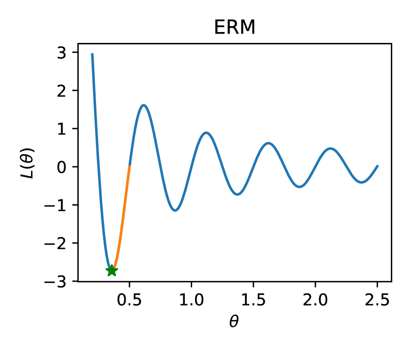
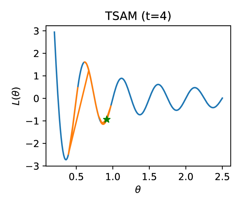
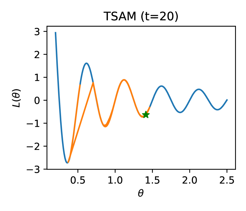
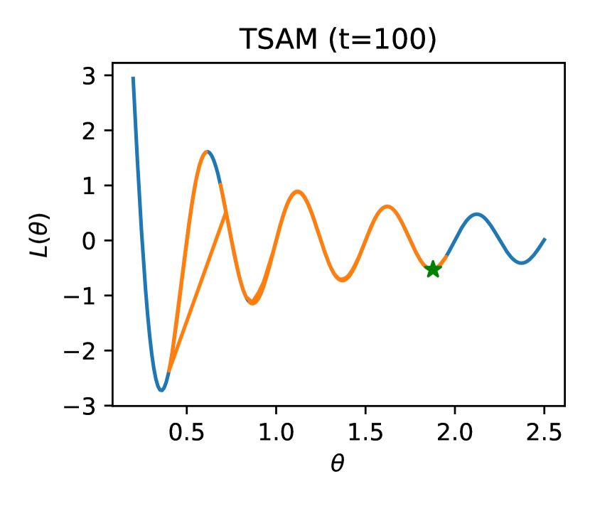
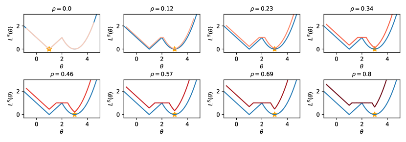
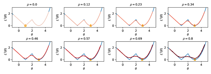
For some sharper than , it is possible that , which implies that ERM is not able to distinguish between the two solutions, while TSAM can. Furthermore, Theorem 1 indicates that as increases, the TSAM objective favors more aggressively, as the gap between and grows larger. We explore a one-dimensional toy problem with many local minima: , and focus on the area to visualize this behavior. We take and a fixed learning rate for all objectives. Each run starts from the same initialization . In Figure 1, we see that as increases, TSAM leads to flatter solutions, despite having larger objective values measured by . As a side note, we prove that for any , the objective value of is monotonically increasing as increases (Appendix B). Next, we discuss a special case when is close to , where we provide another perspective on the TSAM behavior.
Discussions for .
All the results above hold for the small- regime, where sharpness reduces to standard variance when (Definition 2). It still follows that if is sharper than . Here, we provide another interpretation of TSAM when is close to zero. Similar statements have also appeared in prior works in a different context [e.g., 27, 26]. For a very small , it holds that
| (7) |
We provide a proof in Appendix B. Hence, optimizing TSAM is approximately equivalent to optimizing for the mean plus variance of the losses under the perturbed parameters. When , it reduces to only optimizing for . In other words, TSAM with close to 0 is directly minimizing -sharpness (standard variance). For any and such that is sharper than , we have
| (8) | ||||
| (9) |
This is a special case of Theorem 1 for . It suggests that as we increase from 0 for a small amount, the standard variance of neighborhood loss would reduce.
So far, we study properties of TSAM regarding convexity, smoothness of the objective, and sharpness of the resulting solutions. We note that these properties of the objective are independent of the actual optimization algorithms used to optimize TSAM. Though Theorem 1 implies similar benefits of both TSAM and SAM relative to ERM (assuming we optimize TSAM and SAM perfectly), Lemma 2 shows the superiority of the TSAM objective over SAM with unbounded smoothness parameters, as TSAM is easier to optimize. The performance of practical applications depends on both the properties of the objectives and the approximation algorithms used to solve them.
3.3 Generalization of TSAM
In this section, we give a uniform bound on the generalization error of our TSAM objective. By solving the tilted objective empirically, during test time, we are ultimately interested in evaluating the linear population risk where denotes the underlying data distribution and . We define generalization error as the difference between population risk and our empirical objective value , bounded as follows.
Theorem 2 (Generalization of TSAM).
Assume losses are bounded as . Suppose we have training data points. For any and , with probability , the difference between population risk and empirical TSAM risk satisfies
| (10) |
where is a constant independent of .
In other words, we have for any , with probability ,
| (11) |
We defer the proof to Appendix B, where we build upon existing generalization results of a related objective [1]. From Theorem 2, we have multiple interesting observations. (1) When the sample space of is empty, our result reduces to , scaling at a rate of consistent with standard uniform bound on the average risk [40]. (2) When and we define to be over some distribution, the result implies the generalization of SAM: . As , the upper bound of SAM is not smaller than that of ERM. For the most interesting case of , we give a remark on the tightness of the bound below.
Remark 1.
Denote and as optimal solutions for TSAM (Eq. (3)) and ERM (Eq. (1)), respectively. For modest values of , due to the negativity of , the upper bound of the linear population risk (right-hand side of Eq. (11)) can be smaller than that of the linear risk , as long as . This implies that by solving TSAM, we can obtain a solution that gives a smaller linear population error than that of ERM. Following similar arguments, we also see the upper bound of SAM () is larger than that of TSAM under bounded .
In this section, we characterize the upper bound of the population error. In real-world experiments, we also observe there exists an optimal that achieves the best generalization (Section 5).
4 Algorithms
In this section, we describe the algorithms we use to solve TSAM. The main challenge in solving TSAM is to sample to get a good estimator of , or equivalently, . We first describe a general approach where we use estimated tilted gradients (given sampled ’s) to update the model (Section 4.1). Then, we discuss how to sample ’s via a specific Hamiltonian Monte Carlo algorithm and present our method and implementation (Section 4.2).
4.1 General Algorithm
To solve TSAM, the primary challenge is to estimate the integral , or its full gradient , assuming gradient-based methods and the differentiable loss . A naive way is to first sample from following the pre-defined distribution (e.g., Gaussian or uniform) over , and then perform tilted aggregation with weights proportional to . However, this approach may be extremely inefficient, as there could be an infinite set of perturbed model parameters with relatively small losses, which are not informative. In Figure 8 in the appendix, we empirically show that even when we sample a much larger number of ’s, the resulting accuracy is still worse than our proposed method. Instead, we propose to sample number of ’s from distribution (denoted as ), where . We then use these to obtain an empirical gradient estimation with weights proportional to , as the full gradient is a tilted average of the original gradient on . To improve sample efficiency, we use gradient-based methods such as Hamiltonian Monte Carlo (HMC) that simulates Hamiltonian dynamics [24]. The structure of our proposed method is in Algorithm 1. Note that in principle, after estimating the tilted stochastic gradients, we can further apply existing optimization techniques such as variance reduction [19], acceleration [33], or adaptivity [43, 16] to gain further improvement, which we leave for future work.
4.2 Sampling
There could be potentially different algorithms for sampling where . Here we propose an approximate and cheap sampler based on discretization of Hamiltonian dynamics. Our method is inspired by one of the best-known way to approximate the solution to a system of differential equations, i.e., Euler’s method or its modification [32]. A more accurate solver like the leap-frog method might be more popular for HMC, but these come at an increased expense [32]. As our goal to minimize computational cost, we stick with the cheaper Euler’s approach as follows. We first initialize from an ball that satisfies , and initialize the momentum from some Gaussian distribution, i.e., . Note that the negative log probability density of the energy function is . At each sampling step, we run the following steps for iterations with a small step-size to obtain a candidate :
| (12) |
After obtaining a candidate , we accept with probability . If the candidate is not accepted, we set to the initial point before the iterations. Repeating the above for enough times would give us a sample from the exact distribution.
Generating one via HMC requires at least gradient evaluations, which is infeasible for large-scale problems. Hence, we set , and meanwhile accept the generated with probability 1. Combining equations in Eq. (12), if is initialized as , we have , where is a constant absorbing . We adapt this updating rule to our problem, and run the aforementioned procedure in parallel for times to get samples. Our method is presented in Algorithm 2. Though Algorithm 2 does not guarantee the ’s result in a consistent estimator of the TSAM integral, we empirically showcase its effectiveness on non-convex models including transformers in the next section.
5 Experiments
In this section, we first describe our setup. Then we present our main results, comparing TSAM with the baselines of ERM (Eq. (1)), SAM (Eq. (2)), and SAM variants on both image and text data (Section 5.1). We explain TSAM’s superior performance by empirically examining the flatness of local minima in Section 5.2. In Section 5.3, we discuss the effects of hyperparameters.
Tasks and Datasets.
We consider three image tasks involving convolutional neural networks and transformers and the GLUE benchmark of language modeling [46]. First, we explore standard training of ResNet18 [18] on classification over CIFAR100 [22]. Since vision transformers (ViTs) [14] have been shown to have much sharper local minima than CNNs [8], we study the performance on TSAM finetuning ViTs (pretrained on ImageNet [12]) on an out-of-distribution Describable Texture Dataset (DTD) [10], where the task is 47-class classification. Additionally, previous works show that SAM is robust to label noise [17, 4]; and we evaluate in the setting of training ResNet18 on CIFAR100 with uniform label noise generated by substituting 20% of the true labels uniformly at random to other labels. Lastly, we study finetuning a pretrained DistilBert [39] model on the GLUE benchmark including both classification and regression problems on text data. All the experiments are conducted on V100 GPUs with 32GB memory.
Hyperparameter Tuning.
We take to be for all TSAM experiments, and tune the parameters separately from for relevant methods. For TSAM, we tune from and select the best one based on the validation set. We also report the performance for all ’s in the next sections. We use =3 or =5 sampled ’s for all datasets and find that it works well. For some SAM variants that introduce additional hyperparameters, we tune those via grid search as well. We fix the batch size to be 64 for all the datasets and methods, and use constant learning rates tuned from for each algorithm. Despite the existence of adaptive methods for SGD and SAM [20, 23], we do not incorporate adaptivity for any algorithm for a fair comparison. See Appendix C for details.
5.1 TSAM Leads to Better Test Performance
We compare the performance of various objectives and algorithms in Table 1. ERM denotes minimizing the empirical average loss with mini-batch SGD. SAM is the vanilla SAM implementation with one step of gradient ascent and one step of gradient descent at each iteration [17]. Note that TSAM requires more gradient evaluations per iteration. Hence, we include two additional baselines of SAM under the same computational budget as TSAM runs. (1) We simply run the vanilla SAM algorithm for more iterations until it reaches the same runtime as TSAM. (2) We try another SAM approximation by exploring different step sizes along the gradient ascent directions and pick the one incurring the biggest loss. Then we evaluate the gradient under that step size to be applied to the original model parameters. We call these expansive SAM baselines ESAM1, and ESAM2, respectively. We also evaluate two more advanced sharpness-aware optimization methods: PGN that combines normal gradients and SAM gradients [49], and Random SAM (RSAM) which adds random perturbations before finding the adversarial directions [29]. We let PGN and RSAM run the same amount of time as TSAM on the same computing platform. On all the datasets, we tuned values via grid search from .
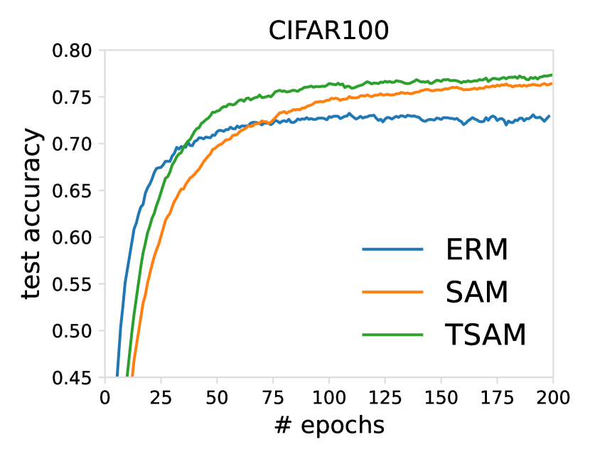
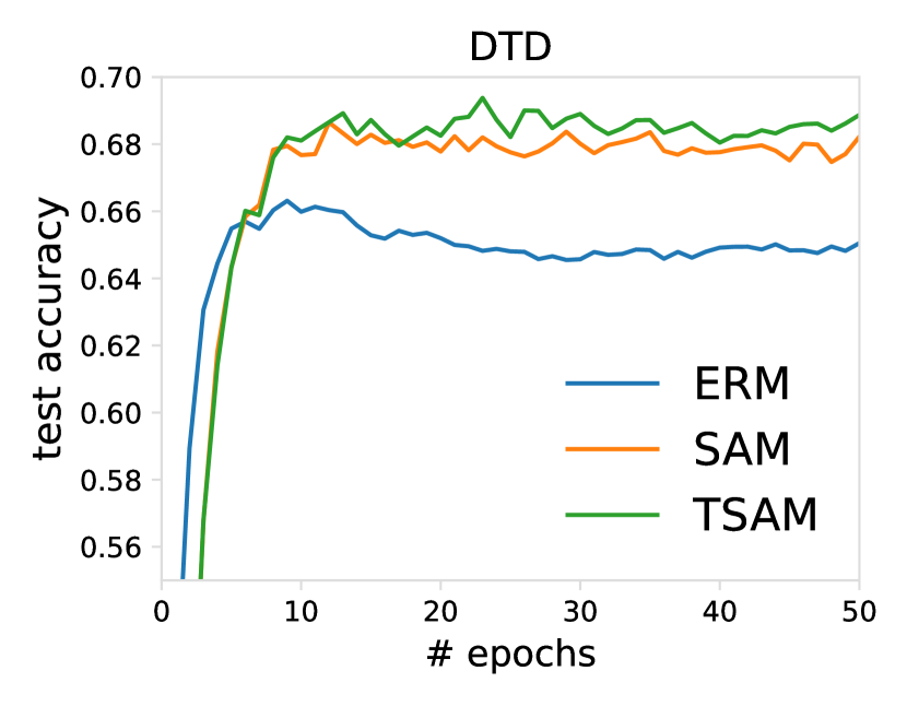
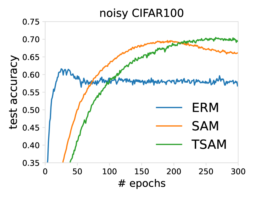
Our results are shown in Table 1 below. The performance for all ’s on three image datasets are reported in Section 5.3. For the GLUE benchmark, we report the standard metrics for each dataset in GLUE. TSAM consistently achieves higher test performance than ERM and variants of SAM. We provide corresponding convergence plots of ERM, vanilla SAM, and TSAM in Appendix C.
| datasets | ERM | SAM | ESAM1 | ESAM2 | PGN | RSAM | TSAM |
|---|---|---|---|---|---|---|---|
| CIFAR100 | 0.7139 | 0.7652 | 0.7740 | 0.7752 | 0.7745 | 0.7735 | 0.7778 |
| DTD | 0.6638 | 0.6787 | 0.6818 | 0.6835 | 0.6776 | 0.6835 | 0.6882 |
| Noisy CIFAR100 | 0.6101 | 0.6900 | 0.6920 | 0.6727 | 0.6568 | 0.6931 | 0.6998 |
| objectives | CoLA | WNLI | SST-2 | MNLI | QNLI | RTE | MRPC | QQP | STSB | AVG |
|---|---|---|---|---|---|---|---|---|---|---|
| ERM | 0.52/0.8034 | 0.5493 | 0.9048 | 0.796 | 0.8772 | 0.6065 | 0.8382 | 0.8632 | 0.866/0.863 | 0.7715 |
| SAM | 0.52/0.8048 | 0.5634 | 0.9174 | 0.811 | 0.8642 | 0.5884 | 0.8529 | 0.8771 | 0.870/0.865 | 0.7756 |
| TSAM | 0.52/0.8081 | 0.5634 | 0.9186 | 0.811 | 0.8781 | 0.6065 | 0.8505 | 0.8877 | 0.871/0.866 | 0.7801 |
5.2 Flatness of TSAM solutions
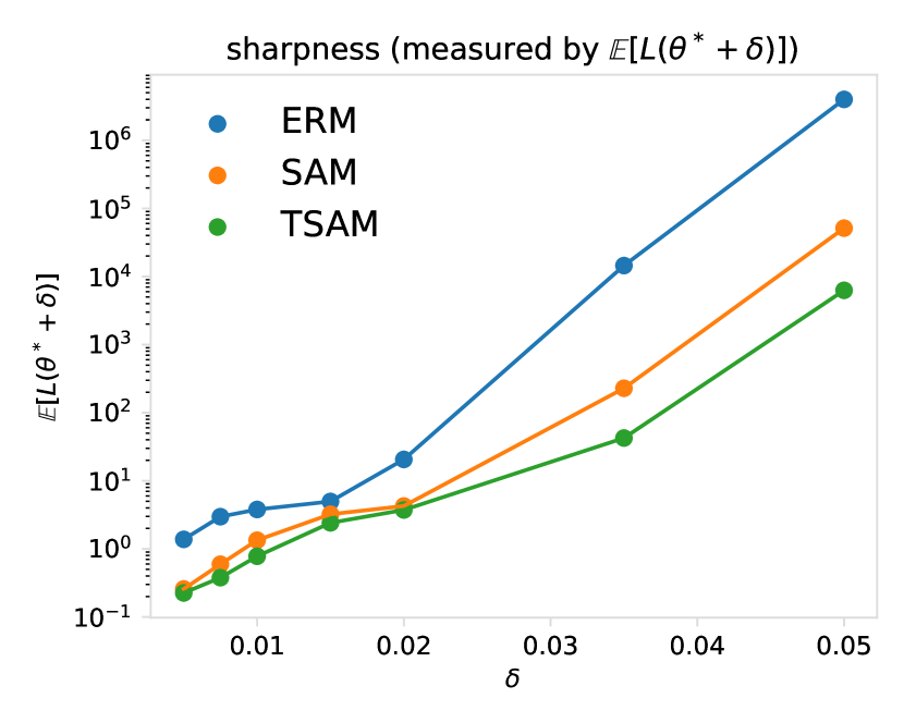
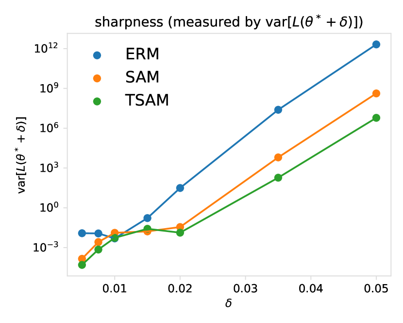
In this part, we take a more detailed look into the properties of TSAM solutions compared with the ones of ERM and SAM on the CIFAR100 dataset trained by ResNet18 from scratch. In Figure 2, we plot the loss mean and variance over the neighborhood areas around local minima obtained by different objectives, i.e., and , where , and denotes the different solutions of any objective (with a slight abuse of notation). These measurements have appeared in prior works [8], and are consistent with our sharpness definition (Definition 3) mentioned before. In Figure 2, for all values, we see that TSAM consistently result in flatter local minima than ERM and SAM measured by both the mean and variance of losses around the minima.
| ERM | SAM | TSAM | |
|---|---|---|---|
| training loss | |||
| ERM | 0.1283 | 1.35 | 3.48 |
| SAM | 0.1489 | 0.22 | 0.60 |
| TSAM | 0.1763 | 0.27 | 0.46 |
| ERM | SAM | TSAM | |
|---|---|---|---|
| test loss | |||
| ERM | 0.9302 | 2.05 | 3.54 |
| SAM | 0.7414 | 0.91 | 1.34 |
| TSAM | 0.7163 | 0.90 | 1.08 |
We further report the training and test performance of best-tuned ERM, SAM, and TSAM in Table 2 CIFAR100 trained by ResNet18. We show that ERM solutions have lower training losses but higher test losses than SAM and TSAM when evaluated on the average test performance (i.e., the ‘ERM’ column in the right table). This is due to the fact that ERM does not generalize as well as SAM or TSAM, and there exist bad sharp local minima around ERM solutions. On the other hand, while TSAM’s average training loss is the highest (which is expected because it does not directly optimize over ERM), the test losses of TSAM evaluated by both the average-case performance and worst-case performance are lower than the other two baselines.
5.3 Sensitivity to Hyperparameters
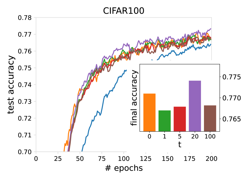
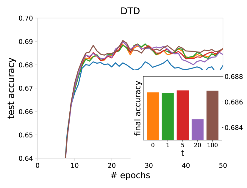
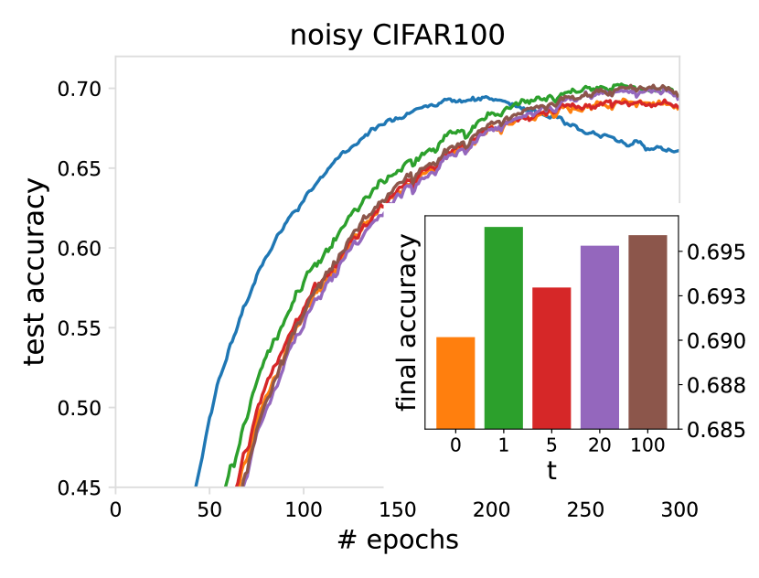
Effects of the Tilting Hyperparameter .
One critial hyperparameter in TSAM is . When , TSAM objective reduces to the SAM objective. When , the TSAM objective (Eq. (3)) recovers SAM (Eq. 2). But the TSAM algorithm (Algorithm 2) do not exactly recover SAM’s alternating updating approximation when . See Section 4 for a detailed discussion. Here, we report the test accuracies as the training proceeds under multiple values of ’s for all the three tasks. Results are plotted in Figure 3. We see that there are a range of ’s that result in faster convergence or higher accuracies than SAM. There also exists an optimal that leads to the best test performance. This is consistent with our previous generalization bound (Section 3.3). Though Theorem 1 captures the benefits of both SAM and TSAM, we note that the final empirical performance does not only depend on the properties of the objectives. But rather, it also relies on the choice of approximation algorithms. Results in Theorem 1 assume that the objectives are optimized perfectly, which is infeasible in high-dimensional settings.

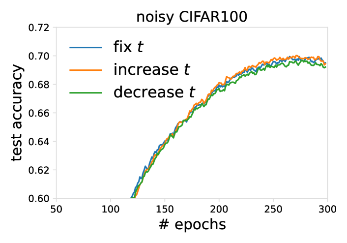
Effects of Scheduling .
We report all results on TSAM where we fix values during optimization. Here, we empirically study the effects of scheduling . Increasing from 0 to a fixed value effectively switches from weighting local minima uniformly to rewighting them based on the loss values, and vice versa. We experiment with two options: linearly decreasing and linearly increasing on the noisy CIFAR100 dataset trained by ResNet18. The convergence curves are shown in Figure 4. We see that using a fixed throughout training does not have significant difference from scheduling . Hence, we stick to fixed ’s for our TSAM experiments.
| CIFAR100 | DTD | noisy CIFAR100 | |
|---|---|---|---|
| SAM | 0.7652 | 0.6787 | 0.6900 |
| TSAM, =3 | 0.7740 | 0.6882 | 0.6955 |
| TSAM, =5 | 0.7778 | 0.6870 | 0.6998 |
Effects of the Number of ’s.
One may wonder whether we need to sample a large number of perturbations for the algorithm to be effective. In Table 5.3, we show that we usually only need or 5 number of ’s to achieve significant improvements relative to SAM.
6 Conclusion
In this work, we have proposed a tilted sharpness-aware minimization (TSAM) objective, which leverages exponential tilting (parameterized by ) to reweight potentially many local minima in the neighborhoods, as opposed to the worst-case minima SAM targets at. We have proved TSAM is a more smooth problem relative to SAM with a bounded , and that TSAM explicitly encourages flatter solutions as increases for a class of problems including generalized linear models. We have proposed a practical algorithm motivated by HMC to sample from the tilted distribution . Through experiments on different models and datasets including label-noise settings, we have demonstrated that TSAM consistently outperforms SAM and its variants on both image and text datasets.
References
- Aminian et al. [2024] Gholamali Aminian, Amir R Asadi, Tian Li, Ahmad Beirami, Gesine Reinert, and Samuel N. Cohen. Generalization error of the tilted empirical risk. arXiv preprint arXiv:2409.19431, 2024.
- Andriushchenko & Flammarion [2022] Maksym Andriushchenko and Nicolas Flammarion. Towards understanding sharpness-aware minimization. In International Conference on Machine Learning, pp. 639–668. PMLR, 2022.
- Andriushchenko et al. [2023] Maksym Andriushchenko, Francesco Croce, Maximilian Müller, Matthias Hein, and Nicolas Flammarion. A modern look at the relationship between sharpness and generalization. arXiv preprint arXiv:2302.07011, 2023.
- Baek et al. [2024] Christina Baek, Zico Kolter, and Aditi Raghunathan. Why is sam robust to label noise? arXiv preprint arXiv:2405.03676, 2024.
- Bartlett et al. [2023] Peter L Bartlett, Philip M Long, and Olivier Bousquet. The dynamics of sharpness-aware minimization: Bouncing across ravines and drifting towards wide minima. Journal of Machine Learning Research, 24(316):1–36, 2023.
- Boucheron et al. [2013] Stéphane Boucheron, Gábor Lugosi, and Pascal Massart. Concentration Inequalities: A Nonasymptotic Theory of Independence. Oxford University Press, 2013.
- Calafiore & El Ghaoui [2014] Giuseppe C Calafiore and Laurent El Ghaoui. Optimization Models. Cambridge University Press, 2014.
- Chen et al. [2021] Xiangning Chen, Cho-Jui Hsieh, and Boqing Gong. When vision transformers outperform resnets without pre-training or strong data augmentations. arXiv preprint arXiv:2106.01548, 2021.
- Chen et al. [2024] Zixiang Chen, Junkai Zhang, Yiwen Kou, Xiangning Chen, Cho-Jui Hsieh, and Quanquan Gu. Why does sharpness-aware minimization generalize better than sgd? Advances in Neural Information Processing Systems, 36, 2024.
- Cimpoi et al. [2014] M. Cimpoi, S. Maji, I. Kokkinos, S. Mohamed, , and A. Vedaldi. Describing textures in the wild. In Proceedings of the IEEE Conf. on Computer Vision and Pattern Recognition (CVPR), 2014.
- Dembo [2009] Amir Dembo. Large deviations techniques and applications. Springer, 2009.
- Deng et al. [2009] Jia Deng, Wei Dong, Richard Socher, Li-Jia Li, Kai Li, and Li Fei-Fei. Imagenet: A large-scale hierarchical image database. In 2009 IEEE conference on computer vision and pattern recognition, pp. 248–255. Ieee, 2009.
- Ding et al. [2024] Lijun Ding, Dmitriy Drusvyatskiy, Maryam Fazel, and Zaid Harchaoui. Flat minima generalize for low-rank matrix recovery. Information and Inference: A Journal of the IMA, 13(2):iaae009, 2024.
- Dosovitskiy et al. [2020] Alexey Dosovitskiy, Lucas Beyer, Alexander Kolesnikov, Dirk Weissenborn, Xiaohua Zhai, Thomas Unterthiner, Mostafa Dehghani, Matthias Minderer, Georg Heigold, Sylvain Gelly, et al. An image is worth 16x16 words: Transformers for image recognition at scale. arXiv preprint arXiv:2010.11929, 2020.
- Du et al. [2022] Jiawei Du, Daquan Zhou, Jiashi Feng, Vincent Tan, and Joey Tianyi Zhou. Sharpness-aware training for free. Advances in Neural Information Processing Systems, 35:23439–23451, 2022.
- Duchi et al. [2011] John Duchi, Elad Hazan, and Yoram Singer. Adaptive subgradient methods for online learning and stochastic optimization. Journal of machine learning research, 12(7), 2011.
- Foret et al. [2020] Pierre Foret, Ariel Kleiner, Hossein Mobahi, and Behnam Neyshabur. Sharpness-aware minimization for efficiently improving generalization. arXiv preprint arXiv:2010.01412, 2020.
- He et al. [2016] Kaiming He, Xiangyu Zhang, Shaoqing Ren, and Jian Sun. Deep residual learning for image recognition. In Proceedings of the IEEE conference on computer vision and pattern recognition, pp. 770–778, 2016.
- Johnson & Zhang [2013] Rie Johnson and Tong Zhang. Accelerating stochastic gradient descent using predictive variance reduction. Advances in neural information processing systems, 26, 2013.
- Kingma & Ba [2014] Diederik P Kingma and Jimmy Ba. Adam: A method for stochastic optimization. arXiv preprint arXiv:1412.6980, 2014.
- Kort & Bertsekas [1972] Barry W Kort and Dimitri P Bertsekas. A new penalty function method for constrained minimization. In Proceedings of the 1972 ieee conference on decision and control and 11th symposium on adaptive processes, pp. 162–166. IEEE, 1972.
- Krizhevsky et al. [2009] Alex Krizhevsky, Geoffrey Hinton, et al. Learning multiple layers of features from tiny images. 2009.
- Kwon et al. [2021] Jungmin Kwon, Jeongseop Kim, Hyunseo Park, and In Kwon Choi. Asam: Adaptive sharpness-aware minimization for scale-invariant learning of deep neural networks. In International Conference on Machine Learning, pp. 5905–5914. PMLR, 2021.
- Leimkuhler & Reich [2004] Benedict Leimkuhler and Sebastian Reich. Simulating hamiltonian dynamics. Number 14. Cambridge university press, 2004.
- Li & Giannakis [2023] Bingcong Li and Georgios Giannakis. Enhancing sharpness-aware optimization through variance suppression. Advances in Neural Information Processing Systems, 36, 2023.
- Li et al. [2023] Tian Li, Ahmad Beirami, Maziar Sanjabi, and Virginia Smith. On tilted losses in machine learning: Theory and applications. Journal of Machine Learning Research, 24(142):1–79, 2023.
- Liu & Theodorou [2019] Guan-Horng Liu and Evangelos A Theodorou. Deep learning theory review: An optimal control and dynamical systems perspective. arXiv preprint arXiv:1908.10920, 2019.
- Liu et al. [2022a] Yong Liu, Siqi Mai, Xiangning Chen, Cho-Jui Hsieh, and Yang You. Towards efficient and scalable sharpness-aware minimization. In Proceedings of the IEEE/CVF Conference on Computer Vision and Pattern Recognition, pp. 12360–12370, 2022a.
- Liu et al. [2022b] Yong Liu, Siqi Mai, Minhao Cheng, Xiangning Chen, Cho-Jui Hsieh, and Yang You. Random sharpness-aware minimization. Advances in Neural Information Processing Systems, 35:24543–24556, 2022b.
- Long & Bartlett [2023] Philip M Long and Peter L Bartlett. Sharpness-aware minimization and the edge of stability. arXiv preprint arXiv:2309.12488, 2023.
- Mi et al. [2022] Peng Mi, Li Shen, Tianhe Ren, Yiyi Zhou, Xiaoshuai Sun, Rongrong Ji, and Dacheng Tao. Make sharpness-aware minimization stronger: A sparsified perturbation approach. Advances in Neural Information Processing Systems, 35:30950–30962, 2022.
- Neal et al. [2011] Radford M Neal et al. Mcmc using hamiltonian dynamics. Handbook of markov chain monte carlo, 2(11):2, 2011.
- [33] Y Nesterov. A method of solving a convex programming problem with convergence rate of . Proceedings of the USSR Academy of Sciences, 269:3.
- Nesterov [1983] Yurii Nesterov. A method for solving the convex programming problem with convergence rate o (1/k2). In Dokl akad nauk Sssr, volume 269, pp. 543, 1983.
- Nesterov [2013] Yurii Nesterov. Introductory lectures on convex optimization: A basic course, volume 87. Springer Science & Business Media, 2013.
- Rice et al. [2021] Leslie Rice, Anna Bair, Huan Zhang, and J Zico Kolter. Robustness between the worst and average case. Advances in Neural Information Processing Systems, 34:27840–27851, 2021.
- Robey et al. [2022] Alexander Robey, Luiz Chamon, George J Pappas, and Hamed Hassani. Probabilistically robust learning: Balancing average and worst-case performance. In International Conference on Machine Learning, pp. 18667–18686. PMLR, 2022.
- Rockafellar et al. [2000] R Tyrrell Rockafellar, Stanislav Uryasev, et al. Optimization of conditional value-at-risk. Journal of risk, 2:21–42, 2000.
- Sanh [2019] V Sanh. Distilbert, a distilled version of bert: Smaller, faster, cheaper and lighter. arXiv preprint arXiv:1910.01108, 2019.
- Shalev-Shwartz & Ben-David [2014] Shai Shalev-Shwartz and Shai Ben-David. Understanding machine learning: From theory to algorithms. Cambridge university press, 2014.
- Shen & Li [2010] Chunhua Shen and Hanxi Li. On the dual formulation of boosting algorithms. IEEE Transactions on Pattern Analysis and Machine Intelligence, 32(12):2216–2231, 2010.
- Siegmund [1976] David Siegmund. Importance sampling in the monte carlo study of sequential tests. The Annals of Statistics, pp. 673–684, 1976.
- Streeter & McMahan [2010] Matthew Streeter and H Brendan McMahan. Less regret via online conditioning. arXiv preprint arXiv:1002.4862, 2010.
- Szabó et al. [2021] Attila Szabó, Hadi Jamali-Rad, and Siva-Datta Mannava. Tilted cross-entropy (tce): Promoting fairness in semantic segmentation. In Proceedings of the IEEE/CVF Conference on Computer Vision and Pattern Recognition, pp. 2305–2310, 2021.
- Wainwright & Jordan [2008] Martin J Wainwright and Michael I Jordan. Graphical models, exponential families, and variational inference. Foundations and Trends® in Machine Learning, 2008.
- Wang [2018] Alex Wang. Glue: A multi-task benchmark and analysis platform for natural language understanding. arXiv preprint arXiv:1804.07461, 2018.
- Wen et al. [2022] Kaiyue Wen, Tengyu Ma, and Zhiyuan Li. How does sharpness-aware minimization minimize sharpness? arXiv preprint arXiv:2211.05729, 2022.
- Wen et al. [2024] Kaiyue Wen, Zhiyuan Li, and Tengyu Ma. Sharpness minimization algorithms do not only minimize sharpness to achieve better generalization. Advances in Neural Information Processing Systems, 36, 2024.
- Zhao et al. [2022] Yang Zhao, Hao Zhang, and Xiuyuan Hu. Penalizing gradient norm for efficiently improving generalization in deep learning. In International Conference on Machine Learning, pp. 26982–26992. PMLR, 2022.
- Zheng et al. [2021] Yaowei Zheng, Richong Zhang, and Yongyi Mao. Regularizing neural networks via adversarial model perturbation. In Proceedings of the IEEE/CVF Conference on Computer Vision and Pattern Recognition, pp. 8156–8165, 2021.
- Zhou et al. [2020] Tianyi Zhou, Shengjie Wang, and Jeff Bilmes. Robust curriculum learning: from clean label detection to noisy label self-correction. In International Conference on Learning Representations, 2020.
- Zhou et al. [2021] Wenxuan Zhou, Fangyu Liu, Huan Zhang, and Muhao Chen. Sharpness-aware minimization with dynamic reweighting. arXiv preprint arXiv:2112.08772, 2021.
- Zhuang et al. [2022] Juntang Zhuang, Boqing Gong, Liangzhe Yuan, Yin Cui, Hartwig Adam, Nicha Dvornek, Sekhar Tatikonda, James Duncan, and Ting Liu. Surrogate gap minimization improves sharpness-aware training. arXiv preprint arXiv:2203.08065, 2022.
Appendix A Additional Toy Problems
In Figure 1 in Section 1, we present a specific toy problem where TSAM arrives at more flat solutions as increases. Though the TSAM objective will recover SAM when , we note that TSAM can be easier to solve due to smoothness. To illustrate this, we create another toy problem in Figure 5 and 6 below. We see that SAM always leads to a non-smooth optimization problem for .
Appendix B Complete Proofs
B.1 Proofs for Section 3.1
Proof for the Case of , .
Note that if is continuously differentiable, then is continuous w.r.t. . It is also continuous w.r.t. . When ,
| (13) | ||||
| (14) | ||||
| (15) | ||||
| (16) |
Proof for Lipschitzness.
First observe that if is -Lipschitz with respect to , then is -Lipschitz with respect to . This follows from
| (17) | ||||
| (18) | ||||
| (19) | ||||
| (20) |
Proof for Strong Convexity.
Assume is continuously differentiable. If is -strongly convex, then is also -strongly convex. This is because of the Hessian in Eq. (21), which can be written as
| (21) |
where is a positive semi-definite matrix. We note that due to the -strong convexity of , the second term satisfies . Hence, .
Proof for Smoothness.
B.2 Proofs for Section 3.2
In the following, we use to denote . Define as
| (24) | ||||
| (25) |
Assume has the specific form of
| (26) | ||||
| (27) |
Under this form, we have that
| (28) | ||||
| (29) | ||||
| (30) |
Define
| (31) |
Then we have
| (32) |
Define
| (33) | ||||
| (34) | ||||
| (35) |
We have that
| (36) |
We know
| (37) | ||||
| (38) |
B.3 is monotonically non-increasing as
We would like to prove the sign of , or , is non-negative. The sign of is the same as the sign of . We have
| (39) | ||||
| (40) |
and
| (41) | ||||
| (42) |
Let random variables , and . Following the fact gives
| (43) |
Therefore
| (44) |
We note that . Hence . Therefore, . we have shown that the tilted SAM loss is monotonically non-decreasing as the increase of , for any .
B.4 -SAM prefers flatter models as increases
Next, we examine .
| (45) | ||||
| (46) | ||||
| (47) |
Similarly,
| (48) |
For ,
| (49) | ||||
| (50) |
Let the random variable denote , and random variable denote . Then
| (51) | |||
| (52) |
Given random variables and , the exponentially reweighted losses can be defined as and . The -weighted second moment is , and the -weighted mean is . Hence, can be viewed as -weighted variance. As is -sharper than , we have . Therefore is non-decreasing as increases. It takes value of when , which implies that .
Proof for the Discussions on .
Recall that and functions can be expanded as
| (53) | ||||
| (54) |
For very small ,
| (55) | |||
| (56) | |||
| (57) | |||
| (58) | |||
| (59) | |||
| (60) |
Hence, our proposed objective can be viewed as optimizing for the mean plus variance of the losses in the neighborhood regions when is very close to 0. When , it reduces to only optimizing for for . For any and such that is sharper than ,
| (61) | ||||
| (62) |
Sharpness is defined in terms of standard variance when (Definition 3), and we have that .
B.5 Proof for Theorem 2
We first state some useful lemmas.
Lemma 3 ([1]).
Let be a random variable. Suppose , we have
| (63) |
The Lemma directly follows from existing results in [1]. For completeness, we include the proof here.
Proof.
As the function is concave for and convex for . Hence, by Jensen’s inequality,
| (64) | ||||
| (65) | ||||
| (66) |
which completes the proof of the lower bound. A similar approach can be applied to derive the upper bound. ∎
Proof for Theorem 2.
We can now proceed with the detailed proof below.
Proof.
Examine the following decomposition of the generalization error
| (67) | |||
| (68) |
Based on Lemma 3, let be and (assuming non-negative and bounded losses and non-negative ), we have that
| (69) |
and
| (70) |
For the term , we further decompose it into
| (71) |
Recall that denote the empirical average loss based on training samples (Eq. (1)), applying Hoeffding Inequality [6] gives
| (72) |
Combining Eq.(70), (71), and (72), we have the desired bound
| (73) | |||
| (74) |
To investigate the impacts of on the generalization bound, we can leave the last term as it is since it is independent of .
Additionally, to bound (the gap between empirical average losses and its randomly-smoothed version) we note that it is related to the curvature of . If we further assume that the loss is -strongly convex, then it holds that
| (75) |
Combining all the above results gives
| (76) |
∎
Appendix C Additional Experimental Details
In this section, we provide additional details on our empirical evaluation.
C.1 Hyperparamter Tuning
We use momentum with a parameter 0.9 for all algorithms. For all the three datasets and all methods, we tune learning rates from . We use a fixed batch size of 64, label smoothing of 0.1 (for smooth cross-entropy loss), momentum with a parameter 0.9, and weight decay 0.0005 for all runs. For vanilla SAM, we tune from and found that the best values are for CIFAR100, DTD, noisy CIFAR100, respectively. For SAM variants, we tune parameters in the same way. The PGN baseline [49] introduces another hyperparameter—the coefficients for the linear combination between normal gradients and SAM gradients, and we tune that from . We follow the recommendations of and hyperparameters in the original Random SAM paper [29]. For TSAM, we set in Algorithm 1, set to be 20, and in Algorithm 2 to be 0.995 across all datasets. We tune from , and the best ’s are 20, 5, 1 for the three image datasets. The number of sampled ’s (the hyperparameter in Algorithm 1) are chosen from . We show the effects of and in detail in Section 5.3 in the main text.
C.2 Convergence Curves
In Table 1, we present the final test accuracies of TSAM and the baseline. In Figure 7, we show the convergence of these methods on three datasets. We see that TSAM achieves the fastest convergence.
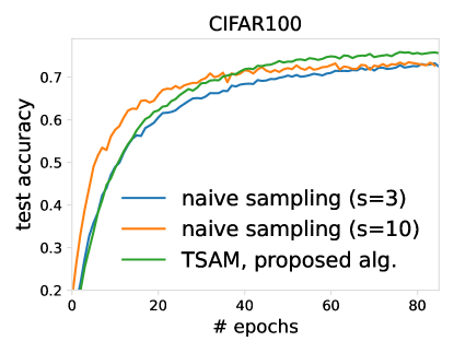
C.3 Naive Sampling
As discussed in Section 4, one naive approach to estimate for in uniformly distributed over is to first uniformly sample ’s over , and then perform tilted aggregation, as follows:
| (77) |
We demonstrate convergence as a function of on the CIFAR100 dataset in the figure below. We see that as increases, the performance increases. However, when , which means that we need 10 gradient evaluations per model updates, the accuracy is lower than that of TSAM with the proposed algorithm.