Inverse of the Gomory Corner Relaxation of Integer Programs

Abstract

We analyze the inverse of the Gomory corner relaxation (GCR) of a pure integer program (IP). We prove the inverse GCR is equivalent to the inverse of a shortest path problem, yielding a polyhedral representation of the GCR inverse-feasible region. We present a linear programming (LP) formulation for solving the inverse GCR under the $L_{1}$ and $L_{\infty}$ norms, with significantly fewer variables and constraints than existing LP formulations for solving the inverse IP in literature. We show that the inverse GCR bounds the inverse IP optimal value as tightly as the inverse LP relaxation under mild conditions. We provide sufficient conditions for the inverse GCR to exactly solve the inverse IP.

Keywords: Inverse optimization; Integer programming; Gomory corner relaxation; Shortest path problem.

1 Introduction

Given a (forward) optimization problem and a feasible solution, the inverse-feasible region is the set of objective vectors under which the given feasible solution is optimal to the forward problem. The inverse optimization problem finds an inverse-feasible vector that is closest (by some given metric) to a given target vector. Inverse optimization has many applications. Tarantola [1] applied inverse optimization in geophysical sciences, such as estimating the epicenter of a seismic event and statistics, e.g., linear regression. Inverse optimization is also useful in estimating liver-transplant patients’ preferences over healthcare outcomes [2], medical imaging [3], cancer treatment [4, 5], estimating the physical properties of solid materials [6], and traffic equilibrium models [7].

The inverse of integer programs (IPs) and the inverse of mixed integer programs (MIPs) have been studied widely. Schaefer [8] and Lamperski and Schaefer [9] established polyhedral representations of the inverse-feasible regions of IPs and MIPs using the superadditive duality of the forward problems. This characterization enabled linear programming (LP) formulations for inverse IPs and inverse MIPs. However, the number of variables and constraints in these LP formulations grow super-exponentially (in the size of the forward problem) and are thus intractable for most instances. Huang [10] reformulated the inverse IP as the inverse of a shortest path problem; the number of vertices and arcs in the graph of this shortest path problem grow super-exponentially (on the number of constraints in the forward IP).

Cutting plane algorithms have been proposed as an alternative to LP formulations for solving inverse IPs and MIPs. Wang [11] provided a cutting plane algorithm for solving inverse MIPs by repeatedly generating optimality cuts from the extreme points of the convex hull of the feasible region of the forward problem. His empirical analysis demonstrated the algorithm’s tractability for small inverse MIPs. The algorithm was improved upon by Duan and Wang [12], who introduced a heuristic algorithm for computing the extreme points and bounds for Wang’s algorithm [11]. Bodur et al. [13] introduced another cutting plane algorithm for solving inverse MIPs, which generates optimality cuts from interior points of the convex hull of the feasible region of the forward problem. Their empirical analysis showed runtime improvements over Wang’s algorithm [11] because the interior points are often easier to compute than the extreme points. These cutting plane algorithms are far more tractable than the LP formulations proposed by Schaefer [8] and Lamperski and Schaefer [9], but the cutting plane algorithms do not characterize the polyhedral structure of the inverse-feasible regions of IPs and MIPs. Inverse IP and inverse MIPs remain theoretically and computationally challenging.

IPs and MIPs are often studied by relaxing the integrality constraints, obtaining the LP relaxation. Therefore, a common approach to studying inverse IP and inverse MIPs is to solve inverse LPs, which typically exhibit more structure. Zhang and Liu [14] proposed a solution for general inverse LPs under the $L_{1}$ norm, from which they obtained strongly polynomial algorithms for solving the inverse minimum cost flow problem and the inverse assignment problem. Zhang and Liu [15] proposed a solution for inverse LPs when both the given feasible solution and an optimal solution under the original objective vector are composed of only zeros and ones, which is common in network flow problems. Ahuja and Orlin [16] showed that if a problem with a linear objective function is polynomially solvable, as is the case for LPs, then the inverse of that problem under the $L_{1}$ or $L_{\infty}$ norm is also polynomially solvable. Tavaslıoğlu et al. [17] studied the polyhedral structure of the inverse-feasible region of LPs, while Chan et al. [18] introduced a goodness-of-fit framework for evaluating inverse LPs where the provided feasible solution for the forward LP problem cannot be made optimal (outside of the trivial zero-objective case).

The Gomory corner relaxation (GCR) is an alternative method for relaxing IPs, obtained by relaxing the nonnegativity constraint of each variable in a basis of the LP relaxation while preserving variable integrality [19]. Gomory [20] noted that the forward GCR reveals the underlying structure of the original IP; for example, the facets of the convex hull of the feasible region of the GCR provide cutting planes for the original IP. Gomory [19], Hoşten and Thomas [21], and Richard and Dey [22] enumerated several classes of IP instances where the optimal solutions for the GCR are also optimal solutions for the original IP. Fischetti and Monaci [23] demonstrated that for many instances, the gap between the IP and GCR optimal values is much tighter than the gap between the IP and LP relaxation optimal values. Köppe et al. [24] characterized the geometry of several reformulations of the GCR. The GCR can be further relaxed to obtain the master group relaxation, which can be applied to broader classes of problems because of its more general structure [22]. The GCR is NP-hard [25], and the most efficient known algorithms for solving the GCR exhibit polynomial runtime complexity with respect to the size of the determinant of the basis matrix of the LP relaxation, which can be very large [25, 22]. Several algorithms for solving the forward GCR reduce the GCR to an instance of the shortest path problem [26, 24, 22], a technique first developed by Shapiro [27].

We show that the inverse GCR can be solved as the inverse of a shortest path problem, which manipulates a graph’s arc weights such that a given path becomes shortest from among all paths that connect the associated origin and destination vertices. The inverse shortest path problem has been extensively studied. The forward shortest path problem can be reduced to a minimum cost flow problem, so the inverse of the shortest path problem under the $L_{1}$ norm can be solved using a strongly polynomial algorithm provided by Zhang and Liu [14]. Ahuja and Orlin [16] showed that the inverse shortest path problem under the $L_{1}$ norm can be reduced to a forward shortest path problem. Zhang et al. [28] proposed a column generation framework for solving a variant of the inverse shortest path problem where several given paths each need to become shortest from among paths that connect their respective origin and destination vertices. Burton and Toint [29] proposed a quadratic programming formulation for solving the inverse shortest path problem under the $L_{2}$ norm. Xu and Zhang [30] characterized the feasible region of the inverse shortest path problem as a polyhedral cone.

We represent the inverse-feasible region of the GCR as a nonempty polyhedral cone and propose an LP formulation for the inverse GCR under the $L_{1}$ and $L_{\infty}$ norms. We show that the inverse GCR bounds the inverse IP optimal value as tightly as the bounds provided by the inverse LP, assuming nondegeneracy. Our formulation of the inverse GCR is much smaller than the exact inverse IP formulation proposed by Schaefer [8].

We study the structure of inverse-feasible regions of IP and GCRs. We demonstrate that solving the inverse of a set of GCR problems, each defined by a different basis of the LP relaxation, provides more information about the inverse of IP than solving only one inverse GCR problem. We also show that the conic hull of the inverse-feasible regions of this set of GCR problems is a subset of the inverse-feasible region of IP. We provide the conditions under which the union of inverse-feasible regions of GCRs is the same as the inverse-feasible region of IP. Additionally, we identify the conditions under which the union of the inverse-feasible regions of GCR is a superset of the inverse-feasible region of the LP relaxation. In the absence of degeneracy, we show that the inverse-feasible region of GCR for some basis always performs as well as the inverse-feasible region of LP relaxation in terms of covering the inverse-feasible region of IP.

2 Preliminaries

2.1 Gomory Corner Relaxation

Given $A\in\mathbb{Z}^{m\times n}$, $b\in\mathbb{Z}^{m}$, and $c\in\mathbb{R}^{n}$, let $\mathcal{IP}$ denote the following IP problem, which we assume has nonempty feasible region. Let $\mathcal{LP}$ denote the LP relaxation of $\mathcal{IP}$:

$$\min\{c^{\intercal}x~{}|~{}Ax=b,x\geq\mathbf{0},x\in\mathbb{Z}^{n}\}, \mathcal{IP}$$ ()

$$\min\{c^{\intercal}x~{}|~{}Ax=b,x\geq\mathbf{0},x\in\mathbb{R}^{n}\}. \mathcal{LP}$$ ()

Let $B,N\subseteq\{1,...,n\}$ respectively denote the indices of the basic and nonbasic variables of a basic solution for $\mathcal{LP}$. Assume $A$ is full row rank and let $m\leq n$, so $|B|=m,|N|=n-m$ and $B\cap N=\varnothing$. Let $c_{B},x_{B}$ $(c_{N},x_{N})$ denote the vectors comprised of the $B$-indexed ($N$-indexed) components of $c,x$, respectively. Let $A_{B}$ ($A_{N}$) be the matrix comprised of the $B$-indexed ($N$-indexed) columns of $A$. Observe that $A_{B}$ is nonsingular. Then, the GCR of $\mathcal{IP}$ with respect to $B$, denoted by $\mathcal{G}^{B}$, is obtained by relaxing the nonnegativity constraints of the decision variables in the selected basis $B$ [22]:

$$\min\{c_{B}^{\intercal}x_{B}+c_{N}^{\intercal}x_{N}~{}|~{}A_{B}x_{B}+A_{N}x_{N}=b,x_{N}\geq\mathbf{0},x\in\mathbb{Z}^{n}\}. \mathcal{G}^{B}$$ ()

For a given $d\in\mathbb{R}^{n}$, let $\mathcal{IP}^{d}$, $\mathcal{LP}^{d}$, $\mathcal{G}^{B,d}$ denote the problems $\mathcal{IP},\mathcal{LP},\mathcal{G}^{B}$, where the original objective vector $c$ has been replaced by $d$. The feasible regions of $\mathcal{IP}^{d}$, $\mathcal{LP}^{d}$, $\mathcal{G}^{B,d}$ remain the same as the feasible regions of the original problems $\mathcal{IP}$, $\mathcal{LP}$, $\mathcal{G}^{B}$, respectively. For a given optimization problem $\mathcal{P}$, let $z(\mathcal{P})$ denote the optimal objective value, and let $Opt(\mathcal{P})$ denote the set of optimal solutions.

Remark 1.

We allow $B$ to be an infeasible basis of $\mathcal{LP}$. Though Gomory [19] also allowed $B$ to be an infeasible basis, he assumed $B$ is an optimal basis to find conditions where solving $\mathcal{G}^{B}$ also solves $\mathcal{IP}$. Richard and Dey [22] and Fischetti and Monaci [23] assumed $B$ is an optimal basis. Allowing $B$ to be an infeasible basis, as done by Köppe et al. [24], permits a more general representation of the inverse GCR. Our results hold for both feasible and infeasible bases of $\mathcal{LP}$. In Section 4.2, we will show if $d$ is in the inverse-feasible region of $\mathcal{G}^{B}$, where $B$ is a feasible basis for $\mathcal{LP}$, then $B$ must be an optimal basis for $\mathcal{LP}^{d}$.

2.2 Gomory Corner Relaxation as a Shortest Path Problem

We summarize how the GCR is reformulated as an instance of the shortest path problem as described by Richard and Dey [22], based on a reformulation first proposed by Shapiro [27].

Lemma 1.

[22] There exist unimodular matrices $S,T\in\mathbb{Z}^{m\times m}$ and a vector $w\in\mathbb{Z}_{+}^{m}$ such that $SA_{B}T=\text{diag}(w)$, where $\text{diag}(w)$ is the $m\times m$ matrix whose diagonal is given by $w$ and whose off-diagonal entries are all zero.

The formulation in Lemma 1 is the Smith Normal Form of $A_{B}$ [31]. There are several efficient algorithms for computing $S$, $T$, and $w$ [32, 33, 34, 35]. $S,T$, and $w$ (as well as several objects we will define later) all depend on the selected basis $B$, but we suppress this dependence on $B$ for clarity.

For a given vector $u\in\mathbb{Z}^{m}$, we define the modulo operator $u(\text{mod}~{}w)$ to denote an $m$-dimensional vector whose $i$th component is given by $(u(\text{mod}~{}w))_{i}=u_{i}\text{ mod }w_{i}$ for each $i\in[m]=\{1,...,m\}$. For example, if $u=(3,5,-2)$ and $w=(2,3,3)$, then $u(\text{mod}~{}w)=(1,2,1)$.

We define linear function $r:\mathbb{R}^{n}\rightarrow\mathbb{R}^{n-m}$ by $r(d)=d_{N}-(A_{B}^{-1}A_{N})^{\intercal}d_{B}$ to denote the reduced costs of the $N$-indexed variables in the basic solution $x_{B}=A_{B}^{-1}b$, $x_{N}=\mathbf{0}$ for $\mathcal{LP}^{d}$. Observe that $r$ depends on the selected basis $B$. We use this notation to define a directed graph $G$ with the vertex set $V$ and the arc set $E$ as follows:

$$V:={\textstyle\prod\limits_{i\in[m]}}\{0,1,...,w_{i}-1\},~{}~{}~{}E:={\textstyle\bigcup\limits_{j\in[n-m]}}E_{j},$$

where, for each $j\in[n-m]$, $(SA_{N})_{j}$ is the $j$th column vector of $SA_{N}$, and

$$E_{j}:=\big{\{}\big{(}u,\big{(}u+(SA_{N})_{j}\big{)}(\text{mod}~{}w)\big{)}~{}|~{}u\in V\big{\}}.$$

Since $S$ and $T$ are unimodular, $\left|\det A_{B}\right|=\prod\limits_{i\in[m]}w_{i}$, and therefore, $|V|=\left|\det A_{B}\right|$ and $|E|=(n-m)\left|\det A_{B}\right|$. Let $\mathcal{S}^{B}$ denote the problem of finding a shortest path from source vertex $\mathbf{0}$ to destination vertex $Sb(\text{mod}~{}w)$ in graph $G$, where each arc in $E_{j}$ is weighted by ${r(c)_{j}}$. For a given $d\in\mathbb{R}^{n}$, let $\mathcal{S}^{B,d}$ denote the same problem of finding a shortest $\mathbf{0}$-to-$Sb(\text{mod}~{}w)$ path in $G$, except each arc in $E_{j}$ is weighted by $r(d)_{j}$ instead of $r(c)_{j}$. Consider any vector $y\in\mathbb{Z}_{+}^{n-m}$. For problem $\mathcal{S}^{B}$, consider all paths that start from source vertex $\mathbf{0}$ and are composed of some permutation of exactly $y_{j}$ arcs from $E_{j}$ for each $j\in[n-m]$. (E.g., if $y=(1,2)$, consider the path that traverses one $E_{1}$ arc then two $E_{2}$ arcs, the path that traverses one $E_{2}$ arc then one $E_{1}$ arc then one $E_{2}$ arc, and the path that traverses two $E_{2}$ arcs then one $E_{1}$ arc.) Such a path always exists because each vertex is the tail of an $E_{j}$ arc for each $j\in[n-m]$. Each $E_{j}$ arc has the same weight $r(c)_{j}$, so all of these paths have the same weight $r(c)^{\intercal}y$. All of these paths also have the same destination vertex $(SA_{N})y~{}(\text{mod}~{}w)$. Thus, if we consider all of these paths to be (possibly infeasible) solutions for $\mathcal{S}^{B}$, then $y$ provides their objective value (path weight $r(c)^{\intercal}y$) and feasibility (if the destination vertex $(SA_{N})y~{}(\text{mod}~{}w)$ is equal to $Sb(\text{mod}~{}w)$). We therefore represent potential solutions for $\mathcal{S}^{B}$ as vectors from $\mathbb{Z}_{+}^{n-m}$, where the vector $y\in\mathbb{Z}_{+}^{n-m}$ corresponds to a path starting at vertex $\mathbf{0}$ that is composed of some permutation of exactly $y_{j}$ arcs from $E_{j}$.

Lemma 2 formalizes the relationship between $\mathcal{G}^{B,d}$ and $\mathcal{S}^{B,d}$ for a given $d\in\mathbb{R}^{n}$. The lemma is given by Richard and Dey [22] for $\mathcal{G}^{B}$ and $\mathcal{S}^{B}$, and their results hold more generally for $\mathcal{G}^{B,d}$ and $\mathcal{S}^{B,d}$ because their proof does not depend on if $B$ is an optimal/feasible basis of the linear relaxation. Their proof offers the following intuition: $x$ is a feasible solution for $\mathcal{G}^{B,d}$ if and only if $x_{N}$ is a $\mathbf{0}$-to-$Sb(\text{mod}~{}w)$ path for $\mathcal{S}^{B,d}$ and $x_{B}=A_{B}^{-1}b-A_{B}^{-1}A_{N}x_{N}$. The objective value of a solution $x$ for $\mathcal{G}^{B,d}$ differs from the weight of the path $x_{N}$ for $\mathcal{S}^{B,d}$ by exactly a fixed value: $d^{\intercal}x=r(d)^{\intercal}x_{N}+c_{B}^{\intercal}A_{B}^{-1}d$.

Lemma 2.

[22] For a given $d\in\mathbb{R}^{n}$, we have $x\in Opt(\mathcal{G}^{B,d})$ if and only if $x_{N}\in Opt(\mathcal{S}^{B,d})$ and $x_{B}=A_{B}^{-1}b-A_{B}^{-1}A_{N}x_{N}$.

We will use this shortest path reformulation $\mathcal{S}^{B}$ of $\mathcal{G}^{B}$ to formulate the inverse GCR as the inverse of a shortest path problem.

2.3 Inverse Optimization

Let $\mathcal{P}$ be an optimization problem from among $\mathcal{IP},\mathcal{LP},\mathcal{G}^{B},\mathcal{S}^{B}$. Let $x^{\circ}$ be a feasible solution for $\mathcal{P}$. The inverse-feasible region of $\mathcal{P}$ with respect to $x^{\circ}$, denoted by $IFR(\mathcal{P},x^{\circ})$, is the set of vectors $d\in\mathbb{R}^{n}$ for which $x^{\circ}$ is an optimal solution for $\mathcal{P}^{d}$:

$$IFR(\mathcal{P},x^{\circ})=\{d\in\mathbb{R}^{n}~{}|~{}x^{\circ}\in Opt(\mathcal{P}^{d})\}.$$

The inverse problem of $\mathcal{P}$ with respect to $x^{\circ}$, denoted by $Inv(\mathcal{P},x^{\circ})$, is the problem of finding a vector $d\in IFR(\mathcal{P},x^{\circ})$ that minimizes the (possibly weighted) $L_{p}$ norm of $d-c$:

$$Inv(\mathcal{P},x^{\circ}): \min\limits\{\lVert d-c\rVert_{p}~{}|~{}d\in IFR(\mathcal{P},x^{\circ})\}.$$

We now give a motivating example where the inverse IP is exactly solved by the inverse GCR but is not exactly solved by the inverse LP relaxation. We later show that generally, the inverse GCR may be easier to compute than the inverse IP while providing a better approximation of the inverse IP than that of the inverse LP relaxation.

Example 1.

Suppose the feasible region of $\mathcal{IP}$ is given by $\{(x_{1},x_{2})\in\mathbb{Z}^{2}~{}|~{}x_{1}+2x_{2}=3,~{}x_{1},x_{2}\geq 0\}=\{(1,1),(3,0)\}$ and $x^{\circ}=(1,1)$. Then, $IFR(\mathcal{IP},x^{\circ})=\{d\in\mathbb{R}^{2}~{}|~{}-2d_{1}+d_{2}\leq 0\}$. The convex hull of the feasible region of $\mathcal{G}^{B}$, $B=\{2\}$ is the ray with origin $x^{\circ}$ and direction $(2,-1)$, so $IFR(\mathcal{G}^{B},x^{\circ})=IFR(\mathcal{IP},x^{\circ})$. $IFR(\mathcal{LP},x^{\circ})=\text{span}\{(1,2)\}$. Thus, $IFR(\mathcal{LP},x^{\circ})\subsetneq IFR(\mathcal{IP},x^{\circ})$ and $Inv(\mathcal{LP},x^{\circ})\geq Inv(\mathcal{G}^{B},x^{\circ})=Inv(\mathcal{IP},x^{\circ})$. $Inv(\mathcal{LP},x^{\circ})>Inv(\mathcal{IP},x^{\circ})$ for many given target objective vectors $c$, including $c\in IFR(\mathcal{IP},x^{\circ})\setminus IFR(\mathcal{LP},x^{\circ})$; see Figure 1.

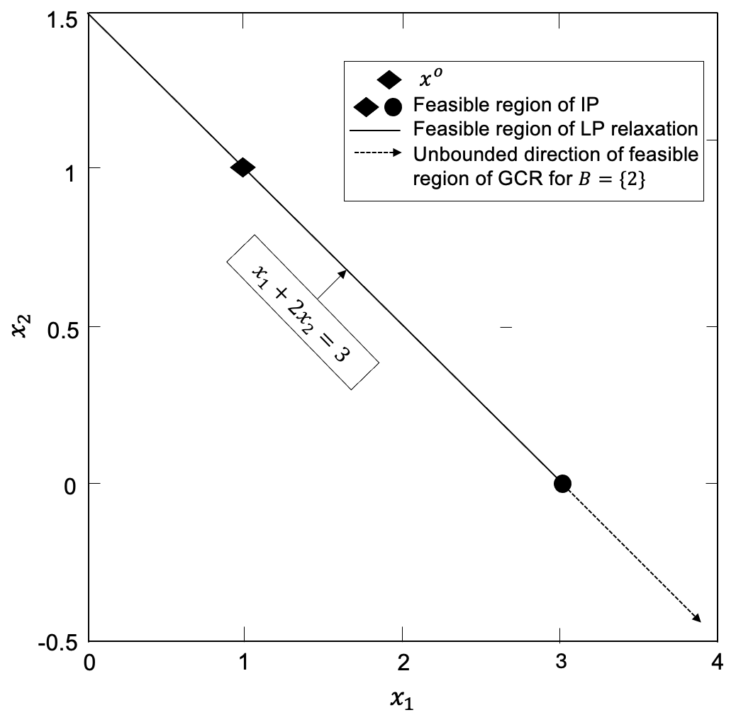
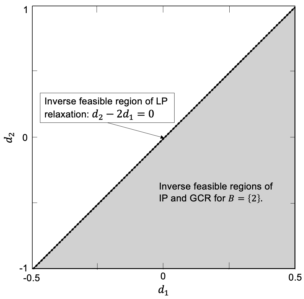
Fig. 1: (Left) The feasible regions of $\mathcal{IP}$, $\mathcal{G}^{B}$ for $B=\{2\}$, $\mathcal{LP}$, and $x^{\circ}=(1,1)$ in Example 1; the feasible region of $\mathcal{IP}$ is shown by the filled diamond at $x^{\circ}=(1,1)$ and the filled circle at $(3,0)$. The feasible region of $\mathcal{G}^{B}$, $B=\{2\}$ is unbounded; The feasible region of $\mathcal{LP}$ is shown by the line segment between $(0,1.5)$ and $(3,0)$. (Right) $IFR(\mathcal{G}^{B},x^{\circ}),IFR(\mathcal{IP},x^{\circ})$, and $IFR(\mathcal{LP},x^{\circ})$ in Example 1, where $IFR(\mathcal{G}^{B},x^{\circ})=IFR(\mathcal{IP},x^{\circ})$ are shown as the shaded region, and $IFR(\mathcal{LP},x^{\circ})$ is shown as the solid line.

3 Characterizing the Inverse of Integer Programs

Let $\mathcal{B}$ be the set of all bases of $\mathcal{LP}$ (both feasible and infeasible), and consider a feasible solution $x^{\circ}$ for $\mathcal{IP}$. For any $B\in\mathcal{B}$, the intersection of the feasible regions of $\mathcal{LP}$ and $\mathcal{G}^{B}$ is exactly the feasible region of $\mathcal{IP}$ because the constraints of $\mathcal{LP}$ enforce nonnegativity and the constraints of $\mathcal{G}^{B}$ enforce integrality. Furthermore, if $\bigcap\limits_{B\in\mathcal{B}}B=\varnothing$, then the intersection of the feasible regions of $\mathcal{G}^{B},B\in\mathcal{B}$ is exactly the feasible region of $\mathcal{IP}$ because the constraints of $\mathcal{G}^{B},B\in\mathcal{B}$ collectively enforce nonnegativity for all decision variables. Thus, it may be possible to obtain large portions of $IFR(\mathcal{IP},x^{\circ})$ using $IFR(\mathcal{LP},x^{\circ})$ and all $IFR(\mathcal{G}^{B},x^{\circ}),B\in\mathcal{B}$.

Though we focus on the inverse of the GCR and its relationship with the inverse LP relaxation, our findings in this section apply to any IP relaxation, such as the master group relaxation [19, 22] or the Lagrangean relaxation [36].

Lemma 3.

Let $x^{\circ}$ be a feasible solution for $\mathcal{IP}$, and let $\mathcal{R}$ be a relaxation of $\mathcal{IP}$. Then, $IFR(\mathcal{R},x^{\circ})\subseteq IFR(\mathcal{IP},x^{\circ})$, and $z(Inv(\mathcal{R},x^{\circ}))\geq z(Inv(\mathcal{IP},x^{\circ}))$.

Proof.

Consider any $d\in IFR(\mathcal{R},x^{\circ})$, so $x^{\circ}\in Opt(\mathcal{R}^{d})$. Since $\mathcal{R}^{d}$ is a relaxation of $\mathcal{IP}^{d}$ and $x^{\circ}$ is a feasible solution for $\mathcal{IP}$, $x^{\circ}\in Opt(\mathcal{IP}^{d})$. Thus, $d\in IFR(\mathcal{IP},x^{\circ})$ and $IFR(\mathcal{R},x^{\circ})\subseteq IFR(\mathcal{IP},x^{\circ})$. $Inv(\mathcal{R},x^{\circ})$ and $Inv(\mathcal{IP},x^{\circ})$ have the same objective function, so $z(Inv(\mathcal{R},x^{\circ}))\geq z(Inv(\mathcal{IP},x^{\circ}))$. ∎

Proposition 1.

Let $x^{\circ}$ be a feasible solution for $\mathcal{IP}$, and let $\mathcal{R}_{1},...,\mathcal{R}_{r}$ be relaxations of $\mathcal{IP}$. Then,

$${\textstyle\bigcup\limits_{i\in[r]}}IFR(\mathcal{R}_{i},x^{\circ})\subseteq\text{cone}(\{IFR(\mathcal{R}_{i},x^{\circ}),i\in[r]\})\subseteq IFR(\mathcal{IP},x^{\circ}).$$

Proof.

Schaefer [8] proved that $IFR(\mathcal{IP},x^{\circ})$ is a polyhedron. Also, $IFR(\mathcal{IP},x^{\circ})$ is a cone because if $d\in IFR(\mathcal{IP},x^{\circ})$, then $td\in IFR(\mathcal{IP},x^{\circ})$ for any $t\in\mathbb{R}_{+}$ [36]. Thus, $IFR(\mathcal{IP},x^{\circ})$ is a polyhedral cone. Clearly, ${\textstyle\bigcup\limits_{i\in[r]}}IFR(\mathcal{R}_{i},x^{\circ})\subseteq\text{cone}(\{IFR(\mathcal{R}_{i},x^{\circ}),i\in[r]\})$. Since, $IFR(\mathcal{IP},x^{\circ})$ is a polyhedral cone and $IFR(\mathcal{R}_{i},x^{\circ})\subseteq IFR(\mathcal{IP},x^{\circ})$ for each $i\in[r]$, we have $\text{cone}(\{IFR(\mathcal{R}_{i},x^{\circ}),i\in[r]\})\subseteq IFR(\mathcal{IP},x^{\circ})$. ∎

From Proposition 1, in cases where ${\textstyle\bigcup\limits_{B\in\mathcal{B}}}IFR(\mathcal{G}^{B},x^{\circ})\neq IFR(\mathcal{IP},x^{\circ})$, we may be able to contain more of $IFR(\mathcal{IP},x^{\circ})$ using the conic hull $\text{cone}(\{IFR(\mathcal{G}^{B},x^{\circ}),B\in\mathcal{B}\})$.

In the following theorem, we show that $IFR(\mathcal{IP},x^{\circ})$ can be fully contained by the inverse-feasible regions of relaxations of $\mathcal{IP}$.

Theorem 1.

Let $x^{\circ}$ be a feasible solution for $\mathcal{IP}$, and let $\mathcal{R}_{1},...,\mathcal{R}_{r}$ be relaxations of $\mathcal{IP}$. Suppose for any selection of one feasible solution for each of $\mathcal{R}_{i},~{}i\in[r]$, there exists a convex combination of those feasible solutions that lies within $\text{conv}(\{Ax=b,x\geq\mathbf{0},x\in\mathbb{Z}^{n}\})$. Then, ${\textstyle\bigcup\limits_{i\in[r]}}IFR(\mathcal{R}_{i},x^{\circ})=IFR(\mathcal{IP},x^{\circ})$.

Proof.

Lemma 3 implies ${\textstyle\bigcup\limits_{i\in[r]}}IFR(\mathcal{R}_{i},x^{\circ})\subseteq IFR(\mathcal{IP},x^{\circ})$. We show $IFR(\mathcal{IP},x^{\circ})\subseteq{\textstyle\bigcup\limits_{i\in[r]}}IFR(\mathcal{R}_{i},x^{\circ})$. By contradiction, suppose there exists $d\in IFR(\mathcal{IP},x^{\circ})\setminus{\textstyle\bigcup\limits_{i\in[r]}}IFR(\mathcal{R}_{i},x^{\circ})$. Then, for each $i\in[r]$, $d\in IFR(\mathcal{IP},x^{\circ})\setminus IFR(\mathcal{R}_{i},x^{\circ})$, so there exists a feasible solution $y^{i}$ for $\mathcal{R}_{i}$ such that $d^{\intercal}y^{i}<d^{\intercal}x^{\circ}$. Let $w$ be the convex combination of $y^{i},i\in[r]$, where $w\in\text{conv}(\{Ax=b,x\geq\mathbf{0},x\in\mathbb{Z}^{n}\})$. Since $w$ is a convex combination of $y^{i},i\in[r]$, we have $d^{\intercal}w<d^{\intercal}x^{\circ}$. Also, since $w\in\text{conv}(\{Ax=b,x\geq\mathbf{0},x\in\mathbb{Z}^{n}\})$ and $d\in IFR(\mathcal{IP},x^{\circ})$, $d^{\intercal}w\geq d^{\intercal}x^{\circ}$. This contradiction indicates that $IFR(\mathcal{IP},x^{\circ})\subseteq{\textstyle\bigcup\limits_{i\in[r]}}IFR(\mathcal{R}_{i},x^{\circ})$. ∎

4 Inverse Gomory Corner Relaxation

4.1 Inverse-Feasible Region of the Shortest Path Reformulation

This subsection provides a polyhedral representation of $IFR(\mathcal{S}^{B},x_{N}^{\circ})$, where $x_{N}^{\circ}$ encodes some given $\mathbf{0}$-to-$Sb(\text{mod}~{}w)$ path. Lemma 4 follows from applying known conditions for a path to be a shortest path to $x_{N}^{\circ}$ for problem $\mathcal{S}^{B,d}$ (e.g., see Chapter 5.2 in Ahuja et al. [37]).

Lemma 4.

For a given $d\in\mathbb{R}^{n}$, $x_{N}^{\circ}$ is a shortest $\mathbf{0}$-to-$Sb(\text{mod}~{}w)$ path for problem $\mathcal{S}^{B,d}$ if and only if for each vertex $u\in V$, there exists an associated $y_{u}\in\mathbb{R}$ such that

$$y_{\mathbf{0}}= ~{}0,$$ (1a)

$$y_{Sb(\text{mod}~{}w)}= ~{}{r(d)}^{\intercal}x_{N}^{\circ},$$ (1b)

$$y_{v}-y_{u}\leq ~{}r(d)_{j}, \forall(u,v)\in E_{j},~{}\forall j\in[n-m].$$ (1c)

$IFR(\mathcal{S}^{B},x_{N}^{\circ})$ is the set of all $d\in\mathbb{R}^{n}$ such that $x^{\circ}_{N}$ is a shortest $\mathbf{0}$-to-$Sb(\text{mod}~{}w)$ path for problem $\mathcal{S}^{B,d}$, so we formulate $IFR(\mathcal{S}^{B},x_{N}^{\circ})$ by defining the set of all $d\in\mathbb{R}^{n}$ that satisfy the conditions in Lemma 4 given by (1a), (1b), (1c).

Proposition 2.

$$IFR(\mathcal{S}^{B},x_{N}^{\circ})=~{} \{d\in\mathbb{R}^{n}~{}|~{}\exists y\in\mathbb{R}^{|V|}\text{~{}such that~{}}\eqref{eq:isp_zero},\eqref{eq:isp_strongdual},\eqref{eq:isp^{d}ualfeasibility}\}$$

$$=~{} \text{proj}_{\mathbb{R}^{n}}\{d\in\mathbb{R}^{n},y\in\mathbb{R}^{|V|}~{}|~{}\eqref{eq:isp_zero},\eqref{eq:isp_strongdual},\eqref{eq:isp^{d}ualfeasibility}\},$$

which is a polyhedral cone that contains $\mathbf{0}$.

Note that $Inv(\mathcal{S}^{B},x_{N}^{\circ})$ is a special case of the general inverse shortest path problem (e.g., studied by Zhang and Liu [14] and Ahuja and Orlin [16]) because each arc in $E_{j}$ has the same weight.

4.2 Feasible Region and Linear Programming Formulation of the Inverse Gomory Corner Relaxation

Theorem 2.

For a given feasible solution $x^{\circ}$ for $\mathcal{G}^{B}$, $IFR(\mathcal{S}^{B},x_{N}^{\circ})=IFR(\mathcal{G}^{B},x^{\circ})$.

Proof. Since $x^{\circ}$ is a feasible solution for $\mathcal{G}^{B}$, we have $x_{B}^{\circ}=A_{B}^{-1}b-A_{B}^{-1}A_{N}x_{N}^{\circ}$. Then, by Lemma 2,

$$d\in IFR(\mathcal{G}^{B},x^{\circ})\iff x^{\circ}\in Opt(\mathcal{G}^{B,d})$$

$$\iff x_{N}^{\circ}\in Opt(\mathcal{S}^{B,d})$$

$$\iff d\in IFR(\mathcal{S}^{B},x_{N}^{\circ}).\hskip 241.84842pt$$

Theorem 2 implies that the inverse GCR is equivalent to the inverse of a shortest path problem, which also implies the GCR inverse-feasible region is a nonempty polyhedral cone by Proposition 2. Most research on the GCR assumes $B$ is an optimal basis of $\mathcal{LP}$ (e.g., [23, 19, 22]). Proposition 3 addresses this condition.

Proposition 3.

Consider a feasible basis $B$ for $\mathcal{LP}$ and a feasible solution $x^{\circ}$ for $\mathcal{G}^{B}$. Then, $B$ is an optimal basis of $\mathcal{LP}^{d}$ for all $d\in IFR(\mathcal{G}^{B},x^{\circ})$.

Proof.

By contradiction, suppose there exists $d\in IFR(\mathcal{G}^{B},x^{\circ})$ such that $B$ is a non-optimal feasible basis of $\mathcal{LP}^{d}$, and let $N=[n]\setminus B$. Non-optimality implies that at least one of the $N$-indexed reduced costs of $\mathcal{LP}^{d}$ must be negative [36]. The arc weights of $\mathcal{S}^{B}$ are defined by the $N$-indexed reduced costs, so there exists $j\in[n-m]$ such that the arcs in $E_{j}$ have negative weight. Since there are finitely many vertices, and each vertex is the tail of an arc from $E_{j}$, we can then construct a negative-weight cycle by repeatedly augmenting a path with arcs from $E_{j}$ until a cycle is formed [22]. The existence of a negative-weight cycle implies $x_{N}^{\circ}$ is not a shortest path, so $d\not\in IFR(\mathcal{S}^{B},x_{N}^{\circ})=IFR(\mathcal{G}^{B},x^{\circ})$. ∎

Corollary 1.

Let $x^{\circ}$ be a feasible solution for $\mathcal{IP}$. Consider a feasible basis $B$ for $\mathcal{LP}$ and the associated basic feasible solution $x_{B}^{*}=A_{B}^{-1}b$, $x_{N}^{*}=\mathbf{0}$. Then, $IFR(\mathcal{G}^{B},x^{\circ})\subseteq IFR(\mathcal{LP},x^{*})$.

We obtain the following LP formulation for $Inv(\mathcal{G}^{B},x^{\circ})$ under the $L_{1}$ norm. The constraints are derived from Proposition 2, and we linearize the objective function $\min\lVert d-c\rVert_{1}$ by substituting $d:=c-e+f$ for $e,f\in\mathbb{R}_{+}^{n}$.

Proposition 4.

For a given feasible solution $x^{\circ}$ for $\mathcal{G}^{B}$, an optimal solution for $Inv(\mathcal{G}^{B},x^{\circ})$ under the $L_{1}$ norm weighted by a given $w\in\mathbb{R}_{+}^{n}$ is equal to $c-e^{*}+f^{*}$, where $e^{*},f^{*},y^{*}$ is an optimal solution for the following LP problem:

$$\min~{} \sum\limits_{k=1}^{n}w_{k}\lparen e_{k}+f_{k}\rparen$$ (2a)

s.t. $$y_{\mathbf{0}}=0,$$ (2b)

$$y_{Sb(\text{mod}~{}w)}=(r(c)-r(e)+r(f))^{\intercal}x_{N}^{\circ},$$ (2c)

$$y_{v}-y_{u}\leq r(c)_{j}-r(e)_{j}+r(f)_{j},\forall(u,v)\in E_{j},~{}\forall j\in[n-m],$$ (2d)

$$e,f\in\mathbb{R}_{+}^{n},~{}y\in\mathbb{R}^{|V|}.$$ (2e)

The LP in (2) can be modified to solve $Inv(\mathcal{G}^{B},x^{\circ})$ under the $L_{\infty}$ norm [16]. The LP formulation for $Inv(\mathcal{G}^{B},x^{\circ})$ can be quite large depending on $\det A_{B}$.

5 Comparing Inverse Formulations

5.1 Comparison with Inverse Linear Programming Relaxation

Theorems 3 and 4 show how the GCR inverse-feasible regions may contain as much of the IP inverse-feasible region as the LP relaxation inverse-feasible region. We compare the optimal values of the inverse IP, inverse GCR, and inverse LP relaxation.

Theorem 3.

Let $x^{\circ}$ $x^{\circ}$ be a feasible solution for $\mathcal{IP}$ that is also a basic feasible solution for $\mathcal{LP}$. Let $\bar{\mathcal{B}}\subseteq\mathcal{B}$ be the set of feasible bases $B$ of $\mathcal{LP}$ that satisfy $x^{\circ}_{B}=A_{B}^{-1}b,x^{\circ}_{N}=\mathbf{0}$. Then, $IFR(\mathcal{LP},x^{\circ})={\textstyle\bigcup\limits_{B\in\bar{\mathcal{B}}}}IFR(\mathcal{G}^{B},x^{\circ}).$

Proof.

By Corollary 1, ${\textstyle\bigcup\limits_{B\in\bar{\mathcal{B}}}}IFR(\mathcal{G}^{B},x^{\circ})\subseteq IFR(\mathcal{LP},x^{\circ})$. To prove $IFR(\mathcal{LP},x^{\circ})\subseteq{\textstyle\bigcup\limits_{B\in\bar{\mathcal{B}}}}IFR(\mathcal{G}^{B},x^{\circ})$, consider any $d\in IFR(\mathcal{LP},x^{\circ})$. Then, $x^{\circ}$ is an optimal solution for $\mathcal{LP}^{d}$, so there exists $B\in\bar{\mathcal{B}}$ such that the reduced costs of the $N$-indexed variables are nonnegative for $\mathcal{LP}^{d}$ [22]. Since $x^{\circ}$ is feasible for $\mathcal{IP}^{d}$, $x^{\circ}$ is also feasible for $\mathcal{G}^{B,d}$, and by Theorem 2, $x^{\circ}_{N}=\mathbf{0}$ is feasible for $\mathcal{S}^{B,d}$. Thus, the source and destination vertices are the same in $\mathcal{S}^{B,d}$, and since the arc weights are defined by the reduced costs of the $N$-indexed variables for $\mathcal{LP}^{d}$, the arc weights are then nonnegative. Therefore, $x^{\circ}_{N}=\mathbf{0}$ is an optimal solution for $\mathcal{S}^{B,d}$. Hence, $x^{\circ}$ is an optimal solution for $\mathcal{G}^{B,d}$, and thus $d\in IFR(\mathcal{G}^{B},x^{\circ})$. ∎

Theorem 4.

Let $x^{\circ}$ be a feasible solution for $\mathcal{IP}$, and let define $K=\{k\in[n]~{}|~{}x^{\circ}_{k}>0\}$.

1. For any basis $B$ of $\mathcal{LP}$ where $B\subseteq K$, we have $IFR(\mathcal{LP},x^{\circ})\subseteq IFR(\mathcal{G}^{B},x^{\circ})$.

2. In the absence of degeneracy, there always exists a feasible basis $B$ such that $B\subseteq K$.

Proof.

Let $B$ be a basis of $\mathcal{LP}$ where $B\subseteq K$. Consider any $d\in\mathbb{R}^{n}$ such that $d\not\in IFR(\mathcal{G}^{B},x^{\circ})$. To prove (a), we will show $IFR(\mathcal{LP},x^{\circ})\subseteq IFR(\mathcal{G}^{B},x^{\circ})$ by proving that $d\not\in IFR(\mathcal{LP},x^{\circ})$, or equivalently, that $x^{\circ}$ is not an optimal solution for $\mathcal{LP}^{d}$. $x^{\circ}$ is not an optimal solution for $\mathcal{G}^{B,d}$, so there exists a feasible solution $y$ for $\mathcal{G}^{B,d}$ such that $d^{\intercal}y<d^{\intercal}x^{\circ}$. We consider two cases.

Case 1. Suppose $y\geq\mathbf{0}$. $y$ is a feasible solution for $\mathcal{G}^{B}$, so $Ay=b$, and therefore $y$ is a feasible solution for $\mathcal{LP}^{d}$. $x^{\circ}$ is not optimal for $\mathcal{LP}^{d}.$

Case 2. Suppose there exist some $k\in B$ such that $y_{k}<0$. Let $C:=\{k\in B~{}|~{}y_{k}<0\}$ denote the indices of the negative components of $y$. We construct $w$ that is a convex combination of $x^{\circ}$ and $y$. Let $\lambda:=\max\{-y_{k}/(x^{\circ}_{k}-y_{k})~{}|~{}k\in C\}$. For each $k\in C$, $x^{\circ}_{k}>0>y_{k}$, so $0<-y_{k}/(x^{\circ}_{k}-y_{k})<1$, which implies $\lambda\in(0,1)$. Let $w:=\lambda x^{\circ}+(1-\lambda)y$. Then, for each $k\in C$, $w_{k}=y_{k}+\lambda(x^{\circ}_{k}-y_{k})\geq y_{k}+(-y_{k}/(x^{\circ}_{k}-y_{k}))(x^{\circ}_{k}-y_{k})=0.$ Also, for each $k\in[n]\setminus C$, we have $x^{\circ}_{k},y_{k}\geq 0$, so $w_{k}\geq 0$. Therefore, $w\geq\mathbf{0}$. Furthermore,

$$d^{\intercal}w=\lambda d^{\intercal}x^{\circ}+(1-\lambda)d^{\intercal}y<\lambda d^{\intercal}x^{\circ}+(1-\lambda)d^{\intercal}x^{\circ}=d^{\intercal}x^{\circ},$$ (3)

and $Aw=A(\lambda x^{\circ}+(1-\lambda)y)=\lambda Ax^{\circ}+(1-\lambda)Ay=b,$ where the last equality holds because both $x^{\circ}$ and $y$ are feasible solutions for $\mathcal{G}^{B,d}$. Thus, $w$ is a feasible solution for $\mathcal{LP}$, and, by (3), $x^{\circ}$ is not an optimal solution for $\mathcal{LP}^{d}$.

To prove (b), define $\delta\in\mathbb{R}^{n}$ by $\delta_{k}=0$ for $k\in K$, and $\delta_{k}=1$ for $k\in[n]\setminus K$. Then, $0\leq z(\mathcal{LP}^{\delta})\leq\delta^{\intercal}x^{\circ}=0$. Thus, $\mathcal{LP}^{\delta}$ has an optimal basis $B^{*}$ associated with the optimal basic solution $x^{*}$ given by $x^{*}_{B^{*}}=A_{B^{*}}^{-1}b$, $x^{*}_{N^{*}}=\mathbf{0}$, where $N^{*}=[n]\setminus B^{*}$. Clearly, $\delta^{\intercal}x^{*}=0$. By contradiction, suppose $B^{*}\not\subseteq K$. Then, there exists $k\in B^{*}\setminus K$ such that $\delta_{k}=1$ because $k\not\in K$, and $x^{*}_{k}>0$ because $k\in B^{*}$, assuming nondegeneracy. We reach the contradiction $0<\delta_{k}x_{k}^{*}\leq\delta^{\intercal}x^{*}=0$. ∎

Corollary 2.

Let $x^{\circ}>\mathbf{0}$ be a feasible solution for $\mathcal{IP}$. Then, $IFR(\mathcal{LP},x^{\circ})\subseteq IFR(\mathcal{G}^{B},x^{\circ})$ for all bases $B$ of $\mathcal{LP}$.

Remark 2.

In Theorem 4, outside of the nondegeneracy condition in part (b), it is possible there does not exist any basis $B$ for $\mathcal{LP}$ such that $B\subseteq K$. For instance, suppose $\mathcal{IP}$ has the feasible region $\{x\in\mathbb{Z}_{+}^{4}~{}|~{}x_{1}+x_{2}+x_{3}-x_{4}=2,x_{1}+x_{2}=2\}$ and $x^{\circ}=(1,1,0,0)$. In this case, $K=\{1,2\}$ indexes two columns of $A$ that are linearly dependent, so there is no basis $B$ of $\mathcal{LP}$ such that $B\subseteq K$.

Remark 3.

In Theorem 4, if $x^{\circ}$ is a feasible solution for $\mathcal{IP}$ that is a nondegenerate basic feasible solution for $\mathcal{LP}$, then $|K|=m$ and so $B=K$ satisfies $IFR(\mathcal{LP},x^{\circ})\subseteq IFR(\mathcal{G}^{B},x^{\circ})$.

Table 1: Comparison of the number of variables and constraints in our LP formulation (2) with Schaefer’s [8] LP formulation for the inverse IP interpretation of the inverse GCR under the $L_{1}$ norm. IP instances were obtained from MIPLIB 2017 [38]. Size of IP Instance lists the number of variables and constraints in the IP instance after converting it to $Ax=b,x\in\mathbb{Z}_{+}^{n}$ form. Inv GCR and Inv IP list the $\log_{10}$ of the number of variables and constraints in our formulation and Schaefer’s [8], respectively.

Size of IP Instance				Inv GCR				Inv IP
Name	var	con			$\log_{10}$ var	$\log_{10}$ con			$\log_{10}$ var	$\log_{10}$ con
gen-ip016	52	24			2.9	4.3			105.8	197.6
gen-ip054	57	27			11.6	13.0			77.6	141.0
gen-ip002	65	24			20.1	21.7			103.1	192.2
gen-ip021	63	28			10.1	11.7			104.6	193.0
ns1952667	13264	41			32.8	36.9			244.5	464.7

5.2 Comparison with Exact Inverse Integer Programming Formulation

Schaefer [8] obtained an exact LP formulation for inverse IPs using superadditive duality, albeit of enormous size. This introduces the question of whether our LP formulation for the inverse GCR in (2) is smaller than solving the inverse GCR as an inverse IP.

We compare the number of variables and constraints in our LP formulation for the inverse GCR in (2) against the number of variables and constraints in Schaefer’s [8] LP formulation for the inverse IP interpretation of the inverse GCR under the $L_{1}$ norm. Table 1 summarizes this comparison for each of five pure IP instances obtained from MIPLIB 2017 [38]. For each instance, $B$ is set to an optimal basis of the LP relaxation, computed using Gurobi 10.0.2 [39]. Our LP formulation has $2n+|\det A_{B}|$ variables and $2+(n-m)|\det A_{B}|$ constraints. Schaefer’s [8] LP formulation has $2n+\prod\limits_{i\in[m]}(|b_{i}|+1)$ variables and $3+n+\prod\limits_{i\in[m]}(|b_{i}|+1)(|b_{i}|+2)-2\prod\limits_{i\in[m]}(|b_{i}|+1)$ constraints.

Our formulation has many magnitudes fewer variables and constraints when compared to Schaefer’s [8] formulation. We conclude that our formulation, which exploits specific GCR properties, yields smaller LP formulations than can be found by solving the inverse GCR as an inverse IP. However, Schaefer’s [8] formulation exactly solves inverse IPs, where our approach only solves the inverse of a relaxation.

6 Conclusion

We formulated the inverse GCR as the inverse of a shortest path problem. We obtained a polyhedral representation of the inverse-feasible region of the GCR, and we proposed an LP formulation for the inverse GCR under the $L_{1}$ and $L_{\infty}$ norms. A GCR inverse-feasible region contains as much of the IP inverse-feasible region as is contained by the LP relaxation inverse-feasible region, in the absence of LP degeneracy. Our formulation of the inverse GCR is much smaller than the exact inverse IP formulation proposed by Schaefer [8].

CRediT

Conceptualization: F. Nosrat, G. Lyu, A. J. Schaefer; Formal analysis: F. Nosrat, A. J. Schaefer; Funding acquisition: A. J. Schaefer; Investigation: F. Nosrat, G. Lyu, A. J. Schaefer; Methodology: F. Nosrat, G. Lyu, A. J. Schaefer; Project administration: F. Nosrat, G. Lyu, A. J. Schaefer; Resources: A. J. Schaefer; Software: F. Nosrat, G. Lyu; Supervision: F. Nosrat, A. J. Schaefer; Visualization: F. Nosrat, G. Lyu; Writing – original draft: F. Nosrat, G. Lyu; Writing - review & editing: F. Nosrat, A. J. Schaefer.

Data availability

No data was used for the research described in the article.

References

- [1] A. Tarantola, Inverse Problem Theory and Methods for Model Parameter Estimation. SIAM: Society for Industrial and Applied Mathematics, 2005.
- [2] Z. Erkin, M. D. Bailey, L. M. Maillart, A. J. Schaefer, and M. S. Roberts, “Eliciting patients’ revealed preferences: An inverse Markov decision process approach,” Decision Analysis, vol. 7, no. 4, pp. 358–365, 2010. https://doi.org/10.1287/deca.1100.0185.
- [3] M. Bertero and M. Piana, Inverse Problems in Biomedical Imaging: Modeling and Methods of Solution. Springer, Milano, 2007.
- [4] T. Ajayi, T. Lee, and A. J. Schaefer, “Objective selection for cancer treatment: An inverse optimization approach,” Operations Research, vol. 70, no. 3, pp. 1717–1738, 2022. https://doi.org/10.1287/opre.2021.2192.
- [5] T. C. Y. Chan, T. Craig, T. Lee, and M. B. Sharpe, “Generalized inverse multiobjective optimization with application to cancer therapy,” Operations Research, vol. 62, no. 3, pp. 680–695, 2014. https://doi.org/10.1287/opre.2014.1267.
- [6] J. C. Brigham, W. Aquino, F. G. Mitri, J. F. Greenleaf, and M. Fatemi, “Inverse estimation of viscoelastic material properties for solids immersed in fluids using vibroacoustic techniques,” Journal of Applied Physics, vol. 101, no. 2, 2007. https://doi.org/10.1063/1.2423227.
- [7] D. Bertsimas, V. Gupta, and I. C. Paschalidis, “Data-driven estimation in equilibrium using inverse optimization,” Mathematical Programming, vol. 153, no. 2, pp. 595–633, 2015. https://doi.org/10.1007/s10107-014-0819-4.
- [8] A. J. Schaefer, “Inverse integer programming,” Optimization Letters, vol. 3, no. 4, pp. 483–489, 2009. https://doi.org/10.1007/s11590-009-0131-z.
- [9] J. B. Lamperski and A. J. Schaefer, “A polyhedral characterization of the inverse-feasible region of a mixed-integer program,” Operations Research Letters, vol. 43, no. 6, pp. 575–578, 2015. https://doi.org/10.1016/j.orl.2015.08.010.
- [10] S. Huang, “Inverse problems of some NP-complete problems,” in Algorithmic Applications in Management: First International Conference, AAIM 2005, pp. 422–426, 2005. https://doi.org/10.1007/11496199_45.
- [11] L. Wang, “Cutting plane algorithms for the inverse mixed integer linear programming problem,” Operations Research Letters, vol. 37, no. 2, pp. 114–116, 2009. https://doi.org/10.1016/j.orl.2008.12.001.
- [12] Z. Duan and L. Wang, “Heuristic algorithms for the inverse mixed integer linear programming problem,” Journal of Global Optimization, vol. 51, no. 3, pp. 463–471, 2011. https://doi.org/10.1007/s10898-010-9637-2.
- [13] M. Bodur, T. C. Y. Chan, and I. Y. Zhu, “Inverse mixed integer optimization: Polyhedral insights and trust region methods,” INFORMS Journal on Computing, vol. 34, no. 3, pp. 1471–1488, 2022. https://doi.org/10.1287/ijoc.2021.1138.
- [14] J. Zhang and Z. Liu, “Calculating some inverse linear programming problems,” Journal of Computational and Applied Mathematics, vol. 72, no. 2, pp. 261–273, 1996. https://doi.org/10.1016/0377-0427(95)00277-4.
- [15] J. Zhang and Z. Liu, “A further study on inverse linear programming problems,” Journal of Computational and Applied Mathematics, vol. 106, no. 2, pp. 345–359, 1999. https://doi.org/10.1016/S0377-0427(99)00080-1.
- [16] R. K. Ahuja and J. B. Orlin, “Inverse optimization,” Operations Research, vol. 49, no. 5, pp. 771–783, 2001. https://doi.org/10.1287/opre.49.5.771.10607.
- [17] O. Tavaslıoğlu, T. Lee, S. Valeva, and A. J. Schaefer, “On the structure of the inverse-feasible region of a linear program,” Operations Research Letters, vol. 46, no. 1, pp. 147–152, 2018. https://doi.org/10.1016/j.orl.2017.12.004.
- [18] T. C. Y. Chan, T. Lee, and D. Terekhov, “Inverse optimization: Closed-form solutions, geometry, and goodness of fit,” Management Science, vol. 65, no. 3, pp. 1115–1135, 2019. https://doi.org/10.1287/mnsc.2017.2992.
- [19] G. Ralph E., “Some polyhedra related to combinatorial problems,” Linear Algebra and its Applications, vol. 2, no. 4, pp. 451–558, 1969. https://doi.org/10.1016/0024-3795(69)90017-2.
- [20] R. E. Gomory, “The atoms of integer programming,” Annals of Operations Research, vol. 149, no. 1, pp. 99–102, 2007. https://doi.org/10.1007/s10479-006-0110-z.
- [21] S. Hoşten and R. R. Thomas, “Gomory integer programs,” Mathematical Programming, vol. 96, no. 2, pp. 271–292, 2003. https://doi.org/10.1007/s10107-003-0386-6.
- [22] J.-P. Richard and S. S. Dey, 50 Years of Integer Programming 1958-2008: From the Early Years to the State-of-the-Art. Springer, 2010. https://doi.org/10.1007/978-3-540-68279-0.
- [23] M. Fischetti and M. Monaci, “How tight is the corner relaxation?,” Discrete Optimization, vol. 5, no. 2, pp. 262–269, 2008. https://doi.org/10.1016/j.disopt.2006.11.010.
- [24] M. Köppe, Q. Louveaux, R. Weismantel, and L. A. Wolsey, “Extended formulations for Gomory corner polyhedra,” Discrete Optimization, vol. 1, no. 2, pp. 141–165, 2004. https://doi.org/10.1016/j.disopt.2004.06.001.
- [25] A. N. Letchford, “Binary clutter inequalities for integer programs,” Mathematical Programming, vol. 98, no. 1, pp. 201–221, 2003. https://doi.org/10.1007/s10107-003-0402-x.
- [26] D.-S. Chen and S. Zionts, “Comparison of some algorithms for solving the group theoretic integer programming problem,” Operations Research, vol. 24, no. 6, pp. 1120–1128, 1976. https://doi.org/10.1287/opre.24.6.1120.
- [27] J. F. Shapiro, “Dynamic programming algorithms for the integer programming problem—I: The integer programming problem viewed as a knapsack type problem,” Operations Research, vol. 16, no. 1, pp. 103–121, 1968. https://doi.org/10.1287/opre.16.1.103.
- [28] J. Zhang, Z. Ma, and C. Yang, “A column generation method for inverse shortest path problems,” Zeitschrift für Operations Research, vol. 41, no. 3, pp. 347–358, 1995. https://doi.org/10.1007/BF01432364.
- [29] D. Burton and P. L. Toint, “On an instance of the inverse shortest paths problem,” Mathematical Programming, vol. 53, no. 1, pp. 45–61, 1992.
- [30] S. Xu and J. Zhang, “An inverse problem of the weighted shortest path problem,” Japan Journal of Industrial and Applied Mathematics, vol. 12, no. 1, pp. 47–59, 1995.
- [31] H. J. S. Smith, “On systems of linear indeterminate equations and congruences,” Philosophical Transactions of the Royal Society of London, vol. 151, pp. 293–326, 1861. https://doi.org/10.1098/rstl.1861.0016.
- [32] S. Birmpilis, G. Labahn, and A. Storjohann, “A fast algorithm for computing the Smith normal form with multipliers for a nonsingular integer matrix,” Journal of Symbolic Computation, vol. 116, pp. 146–182, 2023. https://doi.org/10.48550/arXiv.2111.09949.
- [33] J.-G. Dumas, B. D. Saunders, and G. Villard, “On efficient sparse integer matrix Smith normal form computations,” Journal of Symbolic Computation, vol. 32, no. 1, pp. 71–99, 2001. https://doi.org/10.1006/jsco.2001.0451.
- [34] G. Jäger and C. Wagner, “Efficient parallelizations of Hermite and Smith normal form algorithms,” Parallel Computing, vol. 35, no. 6, pp. 345–357, 2009. https://doi.org/10.1016/j.parco.2009.01.003.
- [35] R. Kannan and A. Bachem, “Polynomial algorithms for computing the Smith and Hermite normal forms of an integer matrix,” SIAM Journal on Computing, vol. 8, no. 4, pp. 499–507, 1979. https://doi.org/10.1137/0208040.
- [36] D. Bertsimas and J. Tsitsiklis, Introduction to Linear Optimization. Athena Scientific and Dynamic Ideas, LLC, 1997.
- [37] R. K. Ahuja, T. L. Magnanti, and J. B. Orlin, Network Flows: Theory, Algorithms, and Applications. Prentice-Hall, 1993.
- [38] A. Gleixner, G. Hendel, G. Gamrath, T. Achterberg, M. Bastubbe, T. Berthold, P. Christophel, K. Jarck, T. Koch, J. Linderoth, M. Lübbecke, H. D. Mittelmann, D. Ozyurt, T. K. Ralphs, D. Salvagnin, and Y. Shinano, “MIPLIB 2017: Data-driven compilation of the 6th mixed integer programming library,” Mathematical Programming Computation, vol. 13, no. 3, pp. 443–490, 2021. https://doi.org/10.1007/s12532-020-00194-3.
- [39] Gurobi Optimization, LLC, “Gurobi Optimizer Reference Manual,” 2023. Accessed: 10-01-2024.