WaveRoRA: Wavelet Rotary Route Attention for Multivariate Time Series Forecasting
Abstract
In recent years, Transformer-based models (Transformers) have achieved significant success in multivariate time series forecasting (MTSF). However, previous works focus on extracting features either from the time domain or the frequency domain, which inadequately captures the trends and periodic characteristics. To address this issue, we propose a wavelet learning framework to model complex temporal dependencies of the time series data. The wavelet domain integrates both time and frequency information, allowing for the analysis of local characteristics of signals at different scales. Additionally, the Softmax self-attention mechanism used by Transformers has quadratic complexity, which leads to excessive computational costs when capturing long-term dependencies. Therefore, we propose a novel attention mechanism: Rotary Route Attention (RoRA). Unlike Softmax attention, RoRA utilizes rotary position embeddings to inject relative positional information to sequence tokens and introduces a small number of routing tokens to aggregate information from the matrices and redistribute it to the matrix, offering linear complexity. We further propose WaveRoRA, which leverages RoRA to capture inter-series dependencies in the wavelet domain. We conduct extensive experiments on eight real-world datasets. The results indicate that WaveRoRA outperforms existing state-of-the-art models while maintaining lower computational costs.
Index Terms:
Time series forecasting, Multivariate time series, Attention mechanism, Rotary position embeddings, Wavelet transform.I Introduction
Multivariate time series (MTS) are prevalent in many real world scenarios, including weather[3], energy management[2], transportation[1] and network flow[9]. Through analyzing historical observations, multivariate time series forecasting (MTSF) aims to extract the underlying patterns of time series data and provides future trends prediction. In the past few years, deep neural networks especially Transformer-based models (Transformers) have achieved great success in MTSF. Transformers rely on the self-attention mechanism[11] to effectively model long-term dependencies in sequences. Models such as Informer[17] and PatchTST[15] make better predictions than previous works that are based on CNNs[5, 4] and RNNs[7]. However, these approaches neglect the correlations between time series, thereby limiting their predictive performance. Some recent works have identified this issue. Models like Sageformer[8] and iTransformer[16] focus on explicitly capturing inter-series dependencies and get superior performance. Nonetheless, the Softmax attention adopted by these models has quadratic computational complexity and may hinder their scalability. Specifically, when modeling intra- or inter-series dependencies, Softmax attention incurs excessive computational costs as the sequence length or the number of variables increases, thus limiting its application in large-scale or high-dimensional scenarios[30, 29, 16].
In addition, existing works mainly focus on analyzing the patterns of MTS data in either time or frequency domains. Features of time domain and frequency domain can reflect different characteristics of the time series. For example, time domain features are conducive to extracting the trends of time series, while frequency domain features reveal the amplitude and phase information of each frequency component of the time series through discrete Fourier transform (DFT)[14]. Compared with time domain features, frequency domain features intuitively reflect the periodicity or seasonality of time series[10]. However, DFT faces the challenges in accurately fitting discontinuous signals, such as abrupt or non-triangular waveforms, which leads to the Gibbs phenomenon[24, 23]. In addition, DFT has limitations in capturing the changes in the frequency domain over time. As shown in Figure 1. Although the three signals exhibit significant differences in the time domain, their frequency spectra are notably similar. Relying exclusively on frequency domain features may result in misleading information and negatively impact the predicting performance of the model. Recent works such as Autoformer[18] and FEDformer[22] introduce frequency-domain features into time-domain representations to facilitate in extracting richer information. However, directly concatenating features of different domains may introduce noise to the model[26], resulting in suboptimal results.
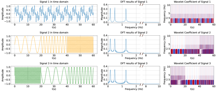
Therefore, we propose to extract features in the wavelet domain. Wavelet transform inherits and develops the localization concept of short-time Fourier transform[6], while overcoming its drawbacks such as the fixed window size that does not vary with different frequencies[27]. Wavelet transform extracts the time-frequency characteristics of a time series by scaling and translating a set of localized wavelet basis functions that decay within a short temporal window. For discrete time series, the Discrete Wavelet Transform (DWT)[25] is typically employed, involving a multi-level wavelet decomposition. As illustrated in Fig. 1, the wavelet coefficients produced from the multi-layer decomposition reflect the different periodic characteristics of the time series and accurately reveal the intervals where different periodic patterns are dominant. Our intuition is that extracting features in the wavelet domain allows us to simultaneously leverage the strengths of both time and frequency domains.
We decompose time series into multi-scale high-pass and low-pass components by using DWT. We design a multi-scale wavelet learning framework to facilitate the mutual conversion between wavelet coefficients and unified-size embeddings, aiming to capture temporal patterns within the time series. We then design a novel Rotary Route Attention mechanism (RoRA) and propose WaveRoRA to capture inter-series dependencies in the wavelet domain. We first use rotary position embeddings to inject relative positional information into and matrices. Subsequently, we introduce a routing tokens , which has much fewer elements than the number of variables. The routing tokens aggregate information from the matrices and redistribute it to the matrix, offering linear complexity. Compared with traditional Softmax attention, RoRA uses the relative positional information to facilitate in identifying the interactions between variables. Meanwhile, the routing tokens effectively alleviate the inherent redundancy between the attention weights and extract critical inter-series dependencies among different variables. Our overall contribution is as follows:
-
•
We propose to model MTS data in the wavelet domain. We design a multi-scale wavelet learning framework to capture temporal patterns within the time series from high-pass and low-pass components obtained by DWT.
-
•
We design a novel RoRA mechanism with linear complexity. We use rotary position embeddings to inject relative position information and introduce a small number of routing tokens to aggregate critical information from the matrices and redistribute it to the matrix.
-
•
Based on the wavelet learning framework and RoRA, we further propose WaveRoRA, which captures inter-series dependencies in the wavelet domain. We conduct extensive experiments on eight real-world datasets. WaveRoRA outperforms existing SOTA models while maintaining low computational costs.
II Related Work
II-A Multivariate Time Series Forecasting
MTSF aims to forecast future values based on a specific period of historical observations[12]. Recently, Transformers achieve great success in MTSF with the Softmax self-attention mechanism[11]. However, the quadratic complexity of sequence length limits these models’ application on MTSF. Researches in recent years thus focus on balancing the predicting performance and computational efficiency of Transformers. LogTrans[13] introduces a local convolutional module in self-attention layers and propose LogSparse attention, which reduces the complexity of . Informer[17] proposes a ProbSparse attention using a distilling technique and selecting top-k elements of the attention weight matrix to achieve complexity. Autoformer[18] designs a decomposition architecture with an Auto-Correlation mechanism. It discovers the sub-series similarity based on the series periodicity and reduce the complexity to . Despite improving forecasting performance and reducing computational costs, these models still rely on point-wise tokens, which limit the receptive field of the input sequence and may lead to overfitting in long-term forecasting. To address this issue, PatchTST[15] generates patch-wise tokens of each univariate series independently and capture intra-series dependencies. It reduces the computational complexity to , where denotes the patch length. The patch-wise tokens facilitates in expanding the receptive field of the input series, leading to better predicting performance. However, PatchTST overlooks the complex interactions between different variables. A recent model named iTransformer [16] generates series-wise tokens and inverts the attention layers to model the inter-series dependencies directly. Although iTransformer achieves superior performance, it still faces high computational costs of when the number of variables is large.
II-B Wavelet Transform
MTS data can be analyzed from various perspectives, such as the time domain, frequency domain, or wavelet domain, each offering unique insights of the underlying patterns of the time series[20]. Generally, the time domain and frequency domain provide intuitive features related to trends and periodic characteristics respectively[19]. Some existing works have explored combining features from these two domains. Autoformer[18] extracts series periods from frequency domain to assist its proposed Auto-correlation in capturing dependencies between periodic segments. FEDformer[22] randomly selects a fixed number of Fourier components to better represent a time series. Through combining Transformer with frequency analysis, FEDformer reduces the computational complexity while leading to performance improvement. However, the Fourier transform struggles to accurately fit discontinuous signals, such as abrupt changes or non-triangular waves. These types of signals are commonly found in real-world scenarios and can cause the Gibbs phenomenon[24, 23].
Analyzing time series in the wavelet domain naturally benefits from its ability to capture both temporal trends in the time domain and periodic patterns in the frequency domain. Wavelet transform decomposes a signal into different frequency and time scales by using scaled and shifted versions of a mother wavelet[25]. In recent years, several researches have been done to explore the effectiveness of modeling time series in the wavelet domain. TCDformer[28] initially encoding abrupt changes using the local linear scaling approximation (LLSA) module and adopt Wavelet Attention to capture temporal dependencies. However, the model uses DWT to directly process point-wise tokens, which causes large computational costs. WaveForM[26], on the contrary, utilizes DWT to map the input series to latent representations in the wavelet domain. It uses dilated convolution and graph convolution modules to further capture the inter-series dependencies[21]. However, WaveForM overlooks the correlation of wavelet coefficients at different levels, which may adversely affect the modeling of the periodic characteristics of time series data.
III Preliminaries
III-A Multivariate Time Series Forecasting
Given a multivariate historical observations with time steps and variables, MTSF aims to predict , where denotes the prediction length.
III-B Discrete Wavelet Transform
DWT decomposes the signals multiple times to generate wavelets at different resolutions. It can capture the local characteristics of signals in both time and frequency domains, enabling localized analysis of temporal trends and frequency patterns.
Generally, DWT decomposes a given signal by using a mother function and a father function , extracting high-pass and low-pass results respectively at varying resolutions, where is the scaling factor that controls the dilation of the wavelet and is the translation factor that shifts the wavelet in time. Specifically, the process of DWT can be defined as Eq 1 and Eq 2, where indicates the -th decomposition, represent the low-pass and high-pass results and , denotes the length of function and and is the length of . The high-pass and low-pass filters are performed convolution operations with the low-pass results of the former layer, generating temporary outputs and . After the convolution, the results will be downsampled by a factor of 2 according to Nyquist theorem, denoted as .
| (1) | ||||
| (2) | ||||
There will be wavelet coefficient outputs after layers of decomposition. Given a multivariate input , each output contains the wavelet coefficient of each variable, denoted as and .
To reconstruct the time series, the Inverse Discrete Wavelet Transform (IDWT) uses the synthesis versions of and , denoted as and , which are time-reversed forms of and . The detailed process of IDWT can be defined in Eq 3:
| (3) | ||||
where is the temporary output, is the low-pass results of the -th layer and represents the upsampling operation. The output of is the final reconstructed sequence in the time domain.
III-C Attention Mechanisms
Given an input sequence where denotes as the number of tokens and represents the token dimension, the attention mechanism can be defined as Eq 4:
| (4) | ||||
where represent the projection matrices and denotes query, key and value matrices respectively. The self-attention[11] uses to produce scaled attention (SA) scores. Such calculation processes lead to complexity.
To address the quadratic computational complexity, a variation of the self-attention mechanism is proposed, namely linear attention (LA)[31]. linear attention is based on the assumption that there exists a kernel function that can approximate the results of . Specifically, the function aims to decouple the parameters of and reformulate it as shown in Eq 5:
| (5) | ||||
where typically. The order of matrix multiplication changes from - pairs to - pairs, leading to complexity. However, linear attention still faces the challenges with excessive computational complexity when dealing with high-dimensional input.
IV Methodology
IV-A Overview
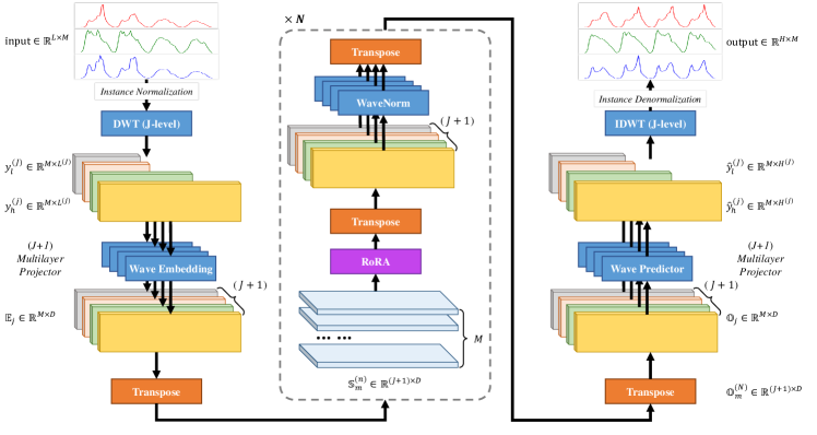
As shown in Fig 2, given the input MTS data , we first apply instance normalization to stabilize the time series. We then apply -level DWT decomposition and get high-pass coefficients and 1 low-pass coefficients . Due to the downsampling during the multi-layer decomposition of DWT, the lengths of the wavelet coefficients of each layer are inconsistent. Therefore, we introduce a set of wave embedding layers to map the multi-layer coefficients to wavelet embeddings with a uniformed size , denoted as , where . After the projection, we transpose into a sequence which is composed of individual variables. We use -layer RoRA to capture the inter-series dependencies in the wavelet domain. To simplify the representation, we omit . For the obtained features of the last layer, we For the obtained features, we flip them again to get . We aim for each element in to correspond to the high-pass and low-pass coefficients obtained after -level wavelet decomposition of the output sequence. Therefore, we again use a set of wave predictor to map them to their corresponding lengths. Finally, we apply IDWT to get the predicted values.
IV-B Instance Normalization
Real-world series usually present non-stationarity[32], resulting in the distribution drift problem[33]. Therefore, we adopt the instance normalization and denormalization technique that is used in Stationary Transformers[32]. Specifically, we record the mean value and variance value of the input series and use them to normalize the input series. When obtaining the output, we apply the same and to denormalize the output series.
IV-C Multi-scale Wave Embedding
The input MTS data is first decomposed to high-pass coefficients and 1 low-pass coefficients with -level DWT, where . Each coefficient series is passed through a corresponding wave embedding layer defined in Eq 6, where and is a linear projector. Specifically, contains a weight matrix and a bias matrix . Note that for and , while . The multi-scale wave embedding layers unify the feature dimensions of wavelet coefficients obtained from the multi-layer DWT. What’s more, the embedding process facilitates in capturing the temporal patterns within the time series.
| (6) | ||||
IV-D Rotary Route Attention
The RoRA is proposed to capture inter-series dependencies in the wavelet domain. We first transpose into a sequence consisting of individual variables. Specifically, we concatenate the wavelet embeddings of each variable to form , where . To simplify the representation, we use as the hidden dimension of each sequence token instead of and denote as the input of RoRA.
| (7) |
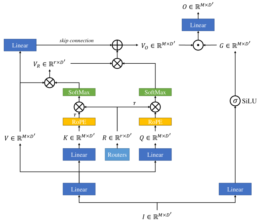
We first utilizes a set of linear projectors to generate query, key and value matrices, represented as , and . Subsequently, a rotary matrix is applied to and to inject relative positional information[34]. Specifically, consists of sub rotary matrices which can be defined in Eq 7. We then randomly initialize a series of routing tokens with a small number of . The route attention can be represented in Eq 8:
| (8) | ||||
where is the function of Softmax attention and refers to the skip connection layer which promotes faster model convergence. The routing tokens is initially viewed as the query for and , aggregating routing features from all keys and values. Afterward, and will serve as the key matrix and value matrix respectively, enabling the transfer of information from the routing features to each query token in . In our implementations, is expected to prune redundant relationships between low-correlation variables while preserving interaction information among high-correlation variables. In addition, we set as a fixed number to achieve linear complexity of relative to the variable number . The complete operation of RoRA mechanism is defined as Eq 9, where corresponds to Eq 8 and refers to Hadamard product. The activation function is set as [36], generating which serves as a gating function.
| (9) | ||||
IV-E Wave-wise Normalization
Considering that the wavelet coefficients of different decomposition layers correspond to different frequency intervals, we transpose the output of RoRA and apply wave-wise normalization for wave embeddings of each decomposition layer. The process corresponds to ”WaveNorm” in Fig 2. Specifically, we calculate and pass each individual through a layer.
IV-F Multi-scale Wavelet Predictor
In order to reconstruct the predicted series with length , the length of high-pass and low-pass coefficients of each decomposition layers input to the IDWT should adhere to the same rules as the DWT process. Specifically, for and , we set and . To map the embeddings to the specific .
For the output of the last RoRA layer, we transpose it to where and pass them through a corresponding MLP individually, as defined in Eq 10:
| (10) | ||||
where , and for , while and . We then input the obtained predicted high-pass and low-pass coefficients to IDWT to get the final outputs .
V Experiments
V-A Datasets
We evaluate our model on 8 real-world datasets: Weather, Electricity, Traffic, Solar and 4 ETT datasets (ETTh1, ETTh2, ETTm1, ETTm2). These datasets are extensively utilized, covering multiple fields including weather, energy management and transportation. The statistics of the datasets are shown in Table I.
| Dataset | Variables | Frequency | Length |
|---|---|---|---|
| Weather | 21 | 10 min | 52696 |
| Electricity | 321 | 1 hour | 26304 |
| Traffic | 862 | 1 hour | 17544 |
| ETTh1 | 7 | 1 hour | 17420 |
| ETTh2 | 7 | 1 hour | 17420 |
| ETTm1 | 7 | 15 min | 69680 |
| ETTm2 | 7 | 15 min | 69680 |
| Solar | 137 | 10min | 52179 |
V-B Baselines
V-C Experiment Settings
We set a uniform input length for all models and conduct experiments with . By default, WaveRoRA employs a 4-level DWT using the Symlet3[25] wavelet basis. We map the wavelet coefficients to embeddings with . For datasets with more variables, such as Weather, Traffic, Electricity and Solar, we construct 3-layer RoRA network, while for datasets with less variables, such as ETT datasets, we set RoRA layer number to 2. For RoRA, we set the token number of to . The attention heads number is set to 8 by default.
We replicate and run PatchTST, iTransformer and DLinear using the publicly available optimal parameters. For other baseline models, we adhere to their established implementations. We record MSE and MAE to measure the performance of different models. All experiments are conducted on one NVIDIA A800 GPU with 40GB memory to exclude the influence of platforms.
| Models | WaveRoRA | iTransformer | PatchTST | Crossformer | Autoformer | Dlinear | TimesNet | |||||||||
|---|---|---|---|---|---|---|---|---|---|---|---|---|---|---|---|---|
| Metric | MSE | MAE | MSE | MAE | MSE | MAE | MSE | MAE | MSE | MAE | MSE | MAE | MSE | MAE | ||
| Weather | 96 | 0.159 | 0.204 | 0.175 | 0.216 | 0.172 | 0.214 | 0.158 | 0.230 | 0.249 | 0.329 | 0.198 | 0.260 | 0.172 | 0.220 | |
| 192 | 0.207 | 0.250 | 0.228 | 0.261 | 0.218 | 0.256 | 0.206 | 0.277 | 0.325 | 0.370 | 0.240 | 0.301 | 0.219 | 0.261 | ||
| 336 | 0.266 | 0.293 | 0.282 | 0.300 | 0.275 | 0.297 | 0.272 | 0.335 | 0.351 | 0.391 | 0.287 | 0.340 | 0.280 | 0.306 | ||
| 720 | 0.347 | 0.345 | 0.360 | 0.350 | 0.352 | 0.347 | 0.398 | 0.418 | 0.415 | 0.426 | 0.353 | 0.395 | 0.365 | 0.359 | ||
| Traffic | 96 | 0.366 | 0.253 | 0.392 | 0.263 | 0.435 | 0.274 | 0.522 | 0.290 | 0.597 | 0.371 | 0.652 | 0.386 | 0.593 | 0.321 | |
| 192 | 0.377 | 0.262 | 0.414 | 0.272 | 0.444 | 0.280 | 0.530 | 0.293 | 0.607 | 0.382 | 0.601 | 0.373 | 0.617 | 0.336 | ||
| 336 | 0.389 | 0.270 | 0.430 | 0.283 | 0.455 | 0.285 | 0.558 | 0.305 | 0.623 | 0.387 | 0.605 | 0.373 | 0.629 | 0.336 | ||
| 720 | 0.424 | 0.289 | 0.452 | 0.297 | 0.488 | 0.304 | 0.589 | 0.328 | 0.639 | 0.395 | 0.649 | 0.399 | 0.640 | 0.350 | ||
| Electricity | 96 | 0.136 | 0.230 | 0.153 | 0.245 | 0.167 | 0.253 | 0.219 | 0.314 | 0.196 | 0.313 | 0.195 | 0.278 | 0.168 | 0.272 | |
| 192 | 0.154 | 0.248 | 0.167 | 0.256 | 0.175 | 0.261 | 0.231 | 0.322 | 0.211 | 0.324 | 0.195 | 0.281 | 0.184 | 0.289 | ||
| 336 | 0.169 | 0.265 | 0.181 | 0.272 | 0.190 | 0.277 | 0.246 | 0.337 | 0.214 | 0.327 | 0.207 | 0.296 | 0.198 | 0.300 | ||
| 720 | 0.198 | 0.296 | 0.219 | 0.305 | 0.236 | 0.314 | 0.280 | 0.363 | 0.236 | 0.342 | 0.242 | 0.328 | 0.220 | 0.320 | ||
| ETTh1 | 96 | 0.384 | 0.403 | 0.394 | 0.410 | 0.380 | 0.399 | 0.423 | 0.448 | 0.435 | 0.446 | 0.391 | 0.403 | 0.384 | 0.402 | |
| 192 | 0.439 | 0.435 | 0.443 | 0.437 | 0.425 | 0.427 | 0.471 | 0.474 | 0.456 | 0.457 | 0.444 | 0.438 | 0.436 | 0.429 | ||
| 336 | 0.473 | 0.454 | 0.485 | 0.460 | 0.464 | 0.445 | 0.570 | 0.546 | 0.486 | 0.487 | 0.480 | 0.463 | 0.491 | 0.469 | ||
| 720 | 0.471 | 0.474 | 0.504 | 0.490 | 0.485 | 0.469 | 0.653 | 0.621 | 0.515 | 0.517 | 0.513 | 0.508 | 0.521 | 0.500 | ||
| ETTh2 | 96 | 0.281 | 0.337 | 0.303 | 0.353 | 0.293 | 0.342 | 0.745 | 0.584 | 0.332 | 0.368 | 0.345 | 0.397 | 0.340 | 0.374 | |
| 192 | 0.357 | 0.387 | 0.385 | 0.401 | 0.383 | 0.396 | 0.877 | 0.656 | 0.426 | 0.434 | 0.473 | 0.472 | 0.402 | 0.414 | ||
| 336 | 0.396 | 0.418 | 0.425 | 0.433 | 0.423 | 0.431 | 1.043 | 0.731 | 0.477 | 0.479 | 0.584 | 0.535 | 0.452 | 0.452 | ||
| 720 | 0.411 | 0.437 | 0.434 | 0.449 | 0.424 | 0.442 | 1.104 | 0.763 | 0.453 | 0.490 | 0.795 | 0.642 | 0.462 | 0.468 | ||
| ETTm1 | 96 | 0.324 | 0.362 | 0.339 | 0.374 | 0.326 | 0.363 | 0.404 | 0.426 | 0.510 | 0.492 | 0.344 | 0.372 | 0.338 | 0.375 | |
| 192 | 0.367 | 0.386 | 0.380 | 0.394 | 0.362 | 0.385 | 0.450 | 0.451 | 0.514 | 0.495 | 0.383 | 0.393 | 0.374 | 0.387 | ||
| 336 | 0.400 | 0.409 | 0.417 | 0.418 | 0.393 | 0.409 | 0.532 | 0.515 | 0.521 | 0.497 | 0.414 | 0.416 | 0.410 | 0.411 | ||
| 720 | 0.466 | 0.444 | 0.478 | 0.452 | 0.451 | 0.439 | 0.666 | 0.589 | 0.537 | 0.513 | 0.474 | 0.452 | 0.478 | 0.450 | ||
| ETTm2 | 96 | 0.172 | 0.255 | 0.189 | 0.274 | 0.177 | 0.261 | 0.287 | 0.366 | 0.205 | 0.293 | 0.190 | 0.287 | 0.187 | 0.267 | |
| 192 | 0.240 | 0.301 | 0.254 | 0.313 | 0.247 | 0.309 | 0.414 | 0.492 | 0.278 | 0.336 | 0.274 | 0.349 | 0.249 | 0.309 | ||
| 336 | 0.301 | 0.339 | 0.315 | 0.352 | 0.312 | 0.351 | 0.597 | 0.542 | 0.343 | 0.379 | 0.376 | 0.421 | 0.321 | 0.351 | ||
| 720 | 0.398 | 0.396 | 0.413 | 0.405 | 0.424 | 0.416 | 1.073 | 1.042 | 0.414 | 0.419 | 0.545 | 0.519 | 0.408 | 0.403 | ||
| Solar | 96 | 0.197 | 0.215 | 0.207 | 0.241 | 0.202 | 0.240 | 0.310 | 0.331 | 0.864 | 0.707 | 0.284 | 0.372 | 0.250 | 0.292 | |
| 192 | 0.231 | 0.252 | 0.240 | 0.264 | 0.240 | 0.265 | 0.734 | 0.725 | 0.844 | 0.695 | 0.320 | 0.396 | 0.296 | 0.318 | ||
| 336 | 0.248 | 0.273 | 0.251 | 0.274 | 0.249 | 0.276 | 0.750 | 0.735 | 0.751 | 0.700 | 0.354 | 0.421 | 0.319 | 0.330 | ||
| 720 | 0.248 | 0.274 | 0.253 | 0.277 | 0.248 | 0.277 | 0.769 | 0.765 | 0.867 | 0.710 | 0.354 | 0.415 | 0.338 | 0.337 | ||
| Models | w/ SA | w/ LA | w/o Ro | w/o Gate | w/o skip | WaveRoRA | iTransformer | |||||||
|---|---|---|---|---|---|---|---|---|---|---|---|---|---|---|
| Metric | MSE | MAE | MSE | MAE | MSE | MAE | MSE | MAE | MSE | MAE | MSE | MAE | MSE | MAE |
| Weather | 0.250 | 0.278 | 0.247 | 0.276 | 0.248 | 0.276 | 0.249 | 0.277 | 0.249 | 0.277 | 0.245 | 0.274 | 0.261 | 0.282 |
| Traffic | 0.400 | 0.275 | 0.426 | 0.280 | 0.396 | 0.271 | 0.405 | 0.276 | 0.393 | 0.270 | 0.389 | 0.269 | 0.422 | 0.279 |
| Electricity | 0.168 | 0.265 | 0.174 | 0.267 | 0.171 | 0.266 | 0.174 | 0.269 | 0.168 | 0.264 | 0.165 | 0.261 | 0.180 | 0.270 |
V-D Main Results
Table II presents all results of MTS forecasting. Compared with the current SOTA Transformer-based model, namely iTransformer, WaveRoRA reduces MSE by 5.53% and MAE by 3.22%. Among all the datasets, WaveRoRA achieves the most improvement on Traffic and Electricity, which contain large amount of variables and exhibit more pronounced periodic characteristics. In particular, the reductions of MSE and MAE come to 7.82% and 3.68% on Traffic and 8.75% and 3.62% on Electricity respectively. Such degree of improvement can be attributed to two aspects: 1) The wavelet transform can accurately model varying periodic patterns over time; 2) The proposed RoRA prunes redundant inter-variable dependencies and retain key information from variables with genuine interactions.
For ETT datasets with less relevancy and non-significant periodicity, capturing inter-series dependencies may negatively impact the predicting accuracy. Models adopting the channel-independent strategy usually achieve better results, such as PatchTST and TimeNet. However, WaveRoRA shows comparable performance to PatchTST on ETTh1 and ETTm1, while achieving more accurate predictions on ETTh2 and ETTm2. This indicates that wavelet transform can effectively preserve time-frequency characteristics and approximate the benefits of time-domain modeling. In addition, we believe that high-quality relative positional information facilitates enhancing interactions between highly correlated variables while weakening those between less correlated ones.
V-E Ablation Study
To justify the effectiveness of our designs, we conduct additional experiments on Weather, Traffic and Electricity. These datasets contains more series data and exhibit better stability. The results are shown in Table III.
V-E1 Wavelet Learning Framework
We replace RoRA with other existing backbones to capture inter-series dependencies, which corresponds to a) w/ SA which uses Softmax attention. Since the wavelet domain embeddings are also generated through an MLP structure, w/ SA can be viewed as replacing the temporal features of iTransformer with wavelet domain features. Compared with iTransformer, w/ SA reduces the MSE by and MAE by on average, which indicates that the wavelet learning framework could provide better predicting results.
V-E2 RoRA structure
To evaluate the effectiveness of the overall structure of RoRA, we further conduct b) w/ LA which uses linear attention to replace RoRA. SA and LA are typical representatives of the attention family, with various attention mechanisms essentially being derivatives of the two. It can be summarized from Table III that w/ SA and w/ LA achieve suboptimal results compared to WaveRoRA, indicating that RoRA has superior representational capacity.
We then conduct c) w/o Ro which removes the rotary positional embeddings, d) w/o Gate which removes the -gating branch and e) w/o skip which removes the skip connection design to evaluate the components of RoRA. After these modules are removed, the predictive performance of the model decreases to varying degrees. The performance decline is most significant in w/o Gate, especially on the Traffic and Electricity datasets, where the MSE and MAE increase by an average of 4.78% and 2.83%. While the routing tokens contribute to prune redundant information, the gating unit further filter out the interaction between weakly correlated variables. The skip connection module preserve historical features and facilitates faster model convergence, therefore, w/o skip gets degraded performance.
V-F Model Efficiency
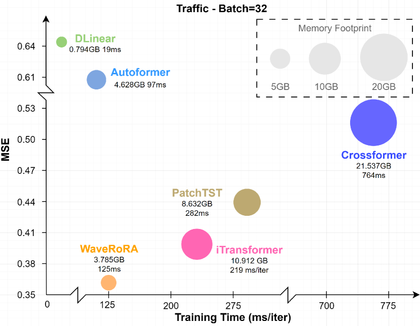
As discussed in section IV-D, RoRA has linear complexity relative to the variable number and the token dimension. To visually demonstrate the efficiency of RoRA, we set batch size to 32 on Traffic and record the training speed and GPU memory usage for WaveRoRA, iTransformer, PatchTST, Autoformer, Crossformer and DLinear. The results are shown in Fig 4, WaveRoRA achieves a good balance among predicting performance, training speed and memory usage.
VI Conclusion
In this paper, we investigate to extract the underlying patterns of MTS data in the wavelet domain. We propose a wavelet learning framework to map the input MTS to wavelet embeddings and capture the inter-series dependencies with a novelly designed RoRA mechanism. The embeddings in the wavelet domain could leverage the strengths of both time and frequency domains, modeling the trends and periodic changing patterns of the time series. What’s more, the proposed RoRA introduces a small number of routing tokens to aggregate information from the matrices and redistribute it to the matrix. Such designs retain the powerful representational capabilities of Softmax and achieve linear complexity relative to both sequence length and token dimension. We conduct extensive experiments and WaveRoRA achieves superior performance compared to SOTA methods. Currently, our wavelet learning framework simply fits for capturing inter-series dependencies, future researches will be done to explore the combination of wavelet domain features with other types of backbones. In addition, we are going to try applying WaveRoRA on more kinds of applications such as Large Time Series Model[38] and AIOPS[37].
References
- [1] S. Guo, Y. Lin, N. Feng, C. Song, and H. Wan, “Attention based spatial-temporal graph convolutional networks for traffic flow forecasting,” in Proceedings of the AAAI conference on artificial intelligence, vol. 33, pp. 922–929, 2019.
- [2] N. Uremović, M. Bizjak, P. Sukič, G. Štumberger, B. Žalik, and N. Lukač, “A new framework for multivariate time series forecasting in energy management system,” IEEE Transactions on Smart Grid, 2022.
- [3] G. Zhang, D. Yang, G. Galanis, and E. Androulakis, “Solar forecasting with hourly updated numerical weather prediction,” Renewable and Sustainable Energy Reviews, vol. 154, p. 111768, 2022.
- [4] H. Wu, T. Hu, Y. Liu, H. Zhou, J. Wang, and M. Long, “Timesnet: Temporal 2d-variation modeling for general time series analysis,” in International Conference on Learning Representations, 2023.
- [5] J. F. Torres, D. Hadjout, A. Sebaa, F. Martínez-Álvarez, and A. Troncoso, “Deep learning for time series forecasting: a survey,” Big Data, vol. 9, no. 1, pp. 3–21, 2021.
- [6] M. Li, Y. Liu, S. Zhi, T. Wang, and F. Chu, “Short-time fourier transform using odd symmetric window function,” Journal of Dynamics, Monitoring and Diagnostics, vol. 1, no. 1, pp. 37–45, 2022.
- [7] D. Liu, J. Wang, S. Shang, and P. Han, “Msdr: Multi-step dependency relation networks for spatial temporal forecasting,” in Proceedings of the 28th ACM SIGKDD conference on knowledge discovery and data mining, pp. 1042–1050, 2022.
- [8] Z. Zhang, L. Meng, and Y. Gu, “Sageformer: Series-aware framework for long-term multivariate time series forecasting,” IEEE Internet of Things Journal, 2024.
- [9] H. Hewamalage, C. Bergmeir, and K. Bandara, “Recurrent neural networks for time series forecasting: Current status and future directions,” International Journal of Forecasting, vol. 37, no. 1, pp. 388–427, 2021.
- [10] Z. Liu, Q. Ma, P. Ma, and L. Wang, “Temporal-frequency co-training for time series semi-supervised learning,” in Proceedings of the AAAI Conference on Artificial Intelligence, vol. 37, pp. 8923–8931, 2023.
- [11] A. Vaswani, N. Shazeer, N. Parmar, J. Uszkoreit, L. Jones, A. N. Gomez, Ł. Kaiser, and I. Polosukhin, “Attention is all you need,” Advances in neural information processing systems, vol. 30, 2017.
- [12] Z. Chen, M. Ma, T. Li, H. Wang, and C. Li, “Long sequence time-series forecasting with deep learning: A survey,” Information Fusion, vol. 97, p. 101819, 2023.
- [13] S. Li, X. Jin, Y. Xuan, X. Zhou, W. Chen, Y.-X. Wang, and X. Yan, “Enhancing the locality and breaking the memory bottleneck of transformer on time series forecasting,” Advances in neural information processing systems, vol. 32, 2019.
- [14] J. W. Cooley and J. W. Tukey, “An algorithm for the machine calculation of complex fourier series,” Mathematics of computation, vol. 19, no. 90, pp. 297–301, 1965.
- [15] Y. Nie, N. H. Nguyen, P. Sinthong, and J. Kalagnanam, “A time series is worth 64 words: Long-term forecasting with transformers,” in The Eleventh International Conference on Learning Representations, ICLR 2023, Kigali, Rwanda, May 1-5, 2023, OpenReview.net, 2023.
- [16] Y. Liu, T. Hu, H. Zhang, H. Wu, S. Wang, L. Ma, and M. Long, “itransformer: Inverted transformers are effective for time series forecasting,” in The Twelfth International Conference on Learning Representations, 2023.
- [17] H. Zhou, S. Zhang, J. Peng, S. Zhang, J. Li, H. Xiong, and W. Zhang, “Informer: Beyond efficient transformer for long sequence time-series forecasting,” in Proceedings of the AAAI conference on artificial intelligence, vol. 35, pp. 11106–11115, 2021.
- [18] H. Wu, J. Xu, J. Wang, and M. Long, “Autoformer: Decomposition transformers with auto-correlation for long-term series forecasting,” Advances in neural information processing systems, vol. 34, pp. 22419–22430, 2021.
- [19] Y. Bai, J. Wang, X. Zhang, X. Miao, and Y. Lin, “Crossfun: Multi-view joint cross fusion network for time series anomaly detection,” IEEE Transactions on Instrumentation and Measurement, 2023.
- [20] X. Zhang, X. Jin, K. Gopalswamy, G. Gupta, Y. Park, X. Shi, H. Wang, D. C. Maddix, and Y. Wang, “First de-trend then attend: Rethinking attention for time-series forecasting,” arXiv preprint arXiv:2212.08151, 2022.
- [21] Z. Wu, S. Pan, G. Long, J. Jiang, X. Chang, and C. Zhang, “Connecting the dots: Multivariate time series forecasting with graph neural networks,” in Proceedings of the 26th ACM SIGKDD international conference on knowledge discovery & data mining, pp. 753–763, 2020.
- [22] T. Zhou, Z. Ma, Q. Wen, X. Wang, L. Sun, and R. Jin, “Fedformer: Frequency enhanced decomposed transformer for long-term series forecasting,” in International conference on machine learning, pp. 27268–27286, PMLR, 2022.
- [23] M. Jiang, P. Zeng, K. Wang, H. Liu, W. Chen, and H. Liu, “Fecam: Frequency enhanced channel attention mechanism for time series forecasting,” Advanced Engineering Informatics, vol. 58, p. 102158, 2023.
- [24] J. W. Gibbs, “Fourier’s series,” Nature, vol. 59, no. 1539, pp. 606–606, 1899.
- [25] I. Daubechies, “Ten lectures on wavelets,” Society for industrial and applied mathematics, 1992.
- [26] F. Yang, X. Li, M. Wang, H. Zang, W. Pang, and M. Wang, “Waveform: Graph enhanced wavelet learning for long sequence forecasting of multivariate time series,” in Proceedings of the AAAI Conference on Artificial Intelligence, vol. 37, pp. 10754–10761, 2023.
- [27] I. Daubechies, “The wavelet transform, time-frequency localization and signal analysis,” IEEE transactions on information theory, vol. 36, no. 5, pp. 961–1005, 1990.
- [28] J. Wan, N. Xia, Y. Yin, X. Pan, J. Hu, and J. Yi, “Tcdformer: A transformer framework for non-stationary time series forecasting based on trend and change-point detection,” Neural Networks, vol. 173, p. 106196, 2024.
- [29] Y. Zhang and J. Yan, “Crossformer: Transformer utilizing cross-dimension dependency for multivariate time series forecasting,” in The eleventh international conference on learning representations, 2023.
- [30] Y. Jia, Y. Lin, X. Hao, Y. Lin, S. Guo, and H. Wan, “Witran: Water-wave information transmission and recurrent acceleration network for long-range time series forecasting,” Advances in Neural Information Processing Systems, vol. 36, 2024.
- [31] A. Katharopoulos, A. Vyas, N. Pappas, and F. Fleuret, “Transformers are rnns: Fast autoregressive transformers with linear attention,” in International conference on machine learning, pp. 5156–5165, PMLR, 2020.
- [32] Y. Liu, H. Wu, J. Wang, and M. Long, “Non-stationary transformers: Exploring the stationarity in time series forecasting,” Advances in Neural Information Processing Systems, vol. 35, pp. 9881–9893, 2022.
- [33] T. Kim, J. Kim, Y. Tae, C. Park, J.-H. Choi, and J. Choo, “Reversible instance normalization for accurate time-series forecasting against distribution shift,” in International Conference on Learning Representations, 2021.
- [34] J. Su, M. Ahmed, Y. Lu, S. Pan, W. Bo, and Y. Liu, “Roformer: Enhanced transformer with rotary position embedding,” Neurocomputing, vol. 568, p. 127063, 2024.
- [35] A. Zeng, M. Chen, L. Zhang, and Q. Xu, “Are transformers effective for time series forecasting?,” in Proceedings of the AAAI conference on artificial intelligence, vol. 37, pp. 11121–11128, 2023.
- [36] S. Elfwing, E. Uchibe, and K. Doya, “Sigmoid-weighted linear units for neural network function approximation in reinforcement learning,” Neural networks, vol. 107, pp. 3–11, 2018.
- [37] J. Diaz-De-Arcaya, A. I. Torre-Bastida, G. Zárate, R. Miñón, and A. Almeida, “A joint study of the challenges, opportunities, and roadmap of mlops and aiops: A systematic survey,” ACM Computing Surveys, vol. 56, no. 4, pp. 1–30, 2023.
- [38] Y. Liu, H. Zhang, C. Li, X. Huang, J. Wang, and M. Long, “Timer: Transformers for time series analysis at scale,” arXiv preprint arXiv:2402.02368, 2024.