An Overtaking Trajectory Planning Framework Based on Spatio-temporal Topology and Reachable Set Analysis Ensuring Time Efficiency

Abstract

Generating overtaking trajectories in high-speed scenarios presents significant challenges and is typically addressed through hierarchical planning methods. However, this method has two primary drawbacks. First, heuristic algorithms can only provide a single initial solution, which may lead to local optima and consequently diminish the quality of the solution. Second, the time efficiency of trajectory refinement based on numerical optimization is insufficient. To overcome these limitations, this paper proposes an overtaking trajectory planning framework based on spatio-temporal topology and reachable set analysis (SROP), to improve trajectory quality and time efficiency. Specifically, this paper introduces topological classes to describe trajectories representing different overtaking behaviors, which support the spatio-temporal topological search method employed by the upper-layer planner to identify diverse initial paths. This approach helps prevent getting stuck in local optima, enhancing the overall solution quality by considering multiple initial solutions from distinct topologies. Moreover, the reachable set method is integrated into the lower-layer planner for parallel trajectory evaluation. This method enhances planning efficiency by decoupling vehicle model constraints from the optimization process, enabling parallel computation while ensuring control feasibility. Simulation results show that the proposed method improves the smoothness of generated trajectories by 66.8% compared to state-of-the-art methods, highlighting its effectiveness in enhancing trajectory quality. Additionally, this method reduces computation time by 62.9%, demonstrating its efficiency.

1 Introduction

As autonomous driving technology continues to evolve, driverless vehicles have greatly enhanced daily travel convenience and demonstrated significant commercial potential. This technology is applied across various scenarios, including fixed-point patrols in factories, freight transport on highways, urban driving, and racing competitions. A common maneuver in these situations is overtaking. In this context, trajectory planning is crucial, as it determines when and how the vehicle should perform an overtaking action. Well-executed trajectory planning guarantees that the vehicle completes the maneuver safely, efficiently, and smoothly, ultimately providing passengers with a superior driving experience.

Trajectory planning typically employs a two-layer hierarchical framework. The upper layer uses heuristic methods to provide reference trajectories for the lower layer, which relies on optimization-based methods to generate trajectories for vehicle control. The upper layer determines a collision-free initial path, primarily addressing which side the vehicle should pass on. Meanwhile, the lower layer refines this initial solution through numerical optimization, ensuring it meets more complex constraints and achieves higher performance requirements. A critical insight of this method is dividing the entire configuration space into a series of non-convex subspaces. The upper-layer search aims to provide the lower-layer trajectory planning with a good initial solution and a non-convex subspace, thereby enhancing the efficiency of trajectory planning. Upper-layer trajectory planning methods generally include sampling and search techniques, which can quickly generate a collision-free initial trajectory. However, these methods have two significant drawbacks. First, trajectories from different topological classes correspond to various overtaking behaviors, and traditional sampling or search methods cannot generate initial trajectories for these diverse classes. Second, since these methods can only produce a single optimal trajectory, they discard other potential trajectories from different topological classes. This limitation significantly reduces the solution space and can lead the lower-layer trajectory planning to become trapped in local optima or fail to find a solution.

To address these issues, this paper proposes an efficient spatio-temporal topological search method. This approach generates a series of collision-free initial paths from different topological classes through graph search. These initial paths act as a skeleton, providing reference values for detailed trajectory optimization at the lower layer. The critical insight is that different topological classes expand the solution space for lower-layer planning. This method can simultaneously consider multiple topological classes, each representing a different non-convex subspace. The advantage is that selecting the best local optimum from these subspaces as the final planning result enhances the solution quality.

The lower-layer trajectory planning method is used to generate a feasible trajectory for a vehicle based on the path identified by the upper layer. This planning method frames the entire trajectory generation problem as a constrained optimization model, which is then solved using numerical methods. It treats the vehicle model as a hard constraint to ensure the feasibility of the trajectory. However, a significant drawback of these methods is that the constraints imposed by the vehicle model can limit the solution space, resulting in a complex and inefficient solving process, or even in cases where no solution exists. This situation can frequently result in unsuccessful overtaking attempts or even serious accidents.

To address this issue, we propose a trajectory generation method based on the reachable set of vehicles, efficiently producing trajectories while ensuring their control feasibility. Specifically, it uses the initial paths provided by the upper-layer search as the reference trajectories. Multiple initial solutions from distinct topologies help prevent getting stuck in local optima, thereby enhancing the overall solution quality. Then, it generates a cluster of candidate trajectories in parallel. Finally, it evaluates the control feasibility of these trajectories using the reachable set method and selects the optimal one as the overtaking trajectory. The key insight of this method is that it decouples trajectory generation from the vehicle model constraints by leveraging the reachable set method. The advantage of this approach is that it avoids the need to solve massive optimization problems, thereby enhancing the efficiency of trajectory optimization while ensuring the control feasibility of the planned trajectories.

1.1 Motivations

Hierarchical methods commonly used for planning overtaking trajectories encounter two main issues that need to be addressed:

• Search-based or sampling-based approaches in the upper layer cannot produce trajectories that reflect diverse overtaking behaviors, which may lead to the planner getting trapped in local optima, reducing the quality of the solution.

• Optimization-based trajectory generation methods in the lower layer face challenges in balancing the efficiency and control feasibility of the generated trajectories.

To tackle the issues mentioned, this paper introduces an overtaking trajectory planning framework based on spatio-temporal topology and reachable set analysis to generate an optimal trajectory that improves the trajectory quality and enhances the time efficiency while ensuring the control feasibility of trajectories. The key innovations are as follows:

1.2 Contributions

The contributions of this paper are summarized as follows:

• An efficient spatio-temporal topological search method is proposed to avoid getting trapped in local optima. This method identifies initial solutions from different topological classes to improve the trajectory quality. Using this method instead of a single initial solution reduces the trajectory tracking error by 19.6% and improves the average smoothness by 20.6%, demonstrating that the proposed method can avoid getting trapped in local optima, thereby improving the solution quality.

• The reachable set and parallel computation are introduced for rapid trajectory planning while ensuring control feasibility. While generating multiple candidate overtaking trajectories, the reachable set is used to perform selection to ensure control feasibility. It provides time efficiency through parallel computation. Compared to the initial trajectory, the tracking error of the overtaking trajectory decreased by 40.3%, confirming the effectiveness of the proposed method in ensuring control feasibility.

• An overtaking trajectory planning framework is proposed to ensure time efficiency and trajectory control feasibility. Compared to state-of-the-art methods, this method demonstrates a 66.8% improvement in trajectory smoothness and a 62.9% reduction in computation time. This validates the effectiveness of the method in improving trajectory quality and planning efficiency.

The remaining paper is organized as follows: Section 2 reviews related work. Section 3 describes relevant notations of reachable set analysis. Section 4 introduces the details of the overtaking trajectory planning framework based on spatio-temporal topology and reachable set analysis. Section 5 presents simulation results, and Section 6 concludes the paper.

2 Related Work

Overtaking trajectory planning in a road involves finding a path for the vehicle between a given start and goal that meets specific constraints and overtakes other vehicles. These constraints include safety (no collisions), minimum time, and minimum energy consumption. The hierarchical planning method is a typical approach to solving the above trajectory planning problem. Such methods generally involve a two-layer planning framework. The upper-layer planner searches for a collision-free initial path, while the lower-layer planner refines the trajectory based on this initial path to meet higher performance requirements [1, 2]. A hierarchical method in [3] includes the front-end trajectory search and back-end optimization based on the convex feasible set algorithm proposed by [4]. A hierarchical method introduced by [5] first searches for an initial path in the spatio-temporal configuration space. Then it transforms the horizontal and vertical optimization problems into a quadratic programming problem to obtain the optimal trajectory. The hierarchical planner proposed by [6] utilizes hybrid A* to search for an initial path in parking scenarios, followed by iterative optimization to convert the collision-free trajectory generation into a quadratic programming problem for rapid solving.

The main planning methods in upper-layer planner include graph search-based methods, sampling-based methods, and their combinations. Specifically, search-based methods, such as A* [7] and Dijkstra [8], are typically employed in partially known static environments. In autonomous driving, A* searches a front-end collision-free trajectory in $s$-$l$-$t$ configuration space [9]. Node expansion in [10] includes vertical and horizontal expansions. Different node combinations represent specific maneuvers, and the optimal trajectory is obtained through an A* search. Search-based methods find it difficult to balance the trade-off between trajectory quality and computation time precisely. As discretization precision increases, solution quality improves, but the computation time grows exponentially. Sampling-based methods are also common approaches for generating initial paths. They usually involve random sampling in the state space. The random sampling methods include the Probabilistic Roadmap (PRM) algorithm [11] and the Rapidly-exploring Random Tree (RRT) algorithm [12]. These methods randomly sample new nodes in the state space, connecting the new sample points with candidate neighbor nodes to form edges for subsequent searches. The trajectory edges between sample nodes can be generated by curve fitting or by solving optimization problems [13, 14, 15].

However, both search-based and sampling-based planning methods can only provide a single initial solution, which may cause subsequent trajectory refinement to become trapped in a local optimum. To overcome this limitation, some research has introduced the concept of path homotopy classes. Obstacles divide the entire planning space into different path topology classes. Each distinct topological trajectory represents an independent decision maneuver [16]. [17] proposed a method to divide the trajectory space into homotopy regions. An efficient topological path searching algorithm is proposed in [18], discovering multiple topological distinct paths in three-dimensional (3D) environments. [16] maintains and optimizes acceptable candidate trajectories of different topologies according to the obstacle environment to seek the best solution. In a 3D static environment, [19] finds a kinematically feasible trajectory through optimization methods from the start to the goal, then translates it in both directions until it does not collide with obstacles. These topological paths serve as reference paths for subsequent kinodynamic RRT* growth. [20] considers time information when searching for different homotopies to handle dynamic obstacles, which distinguishes it from [18] and [19].

Optimization-based methods in the lower layer planner are commonly used for trajectory refinement. In [21], static and dynamic obstacles are segmented using polygons, and then sequential quadratic programming methods are used to generate the trajectory. Gu et al. [22] sample an initial path in the state space and then optimize the selected curve further to obtain a feasible trajectory. [23] uses a Mixed-Integer Quadratic Program to formulate trajectory planning while considering multiple logical constraints on the road. The literature [24] utilizes signed distance approximations to create constraints on other moving vehicles. Model predictive control (MPC) methods are also commonly used for trajectory refinement. Some linearized Model Predictive Control (LMPC) methods can simplify trajectory planning problems. For instance, [25, 26, 27] linearize the vehicle model and constraints to speed up solving the problem. However, this linearization can cause significant model errors, which may result in collisions. In contrast, nonlinear MPC (NMPC) methods can handle more complex optimization problems. [28] integrates a dynamic vehicle model, while [29] considers the constraint of trajectory curvature. These nonlinear terms increase the complexity of the problem. Nevertheless, these NMPC models can lead to longer solution times, making them unsuitable for scenarios that require high real-time performance. Optimization-based methods struggle to balance computational efficiency with solution accuracy. Simplified optimization problems improve computational efficiency but may produce infeasible trajectories. In contrast, complex optimization problems can ensure trajectory control feasibility, yet they are highly computationally inefficient.

By temporarily disregarding the vehicle model in trajectory generation, time efficiency can be significantly improved. This can be accomplished by utilizing the reachable set of vehicles. The reachable set refers to the collection of all possible states a dynamic system can achieve under bounded constraints, starting from an initial state. In [30], the reachable set is the collection of motion states that a vehicle can reach at any given moment while satisfying kinematic constraints. The reachable set provides a continuous drivable area. Areas outside this set represent states that do not meet the kinematic limits of vehicles. To enhance computational efficiency, [31] simplify the vehicle model to a point mass model to compute the reachable sets. The drivable corridor at any moment is formed by the union of the Cartesian products of the $x$ and $y$ directions, resulting in a 2D convex polytope. [32] effectively reduces the search space and significantly lowers the dimensionality of sampling by the reachable set. [33, 34] extract the driving corridors and generate a trajectory within these polygons using convex optimization methods. [35] integrate the kinematic vehicle model and account for uncertainties in state and input, forming a series of reachable sets. Since the reachable set represents all states that the vehicle can achieve under constrained inputs, we can evaluate the control feasibility of a trajectory by examining the relationship between the trajectory and the corresponding reachable set.

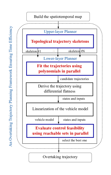
Figure 1: The overall architecture of the overtaking trajectory planning framework

This paper proposes an overtaking trajectory planning framework based on spatio-temporal topology and reachable set analysis, to improve the trajectory quality and time efficiency. Specifically, the upper-layer planner searches for reference skeletons of different topological types. These skeletons provide diverse initial solutions for refinement of the lower-layer planner, helping to avoid local optima and improve trajectory quality. The lower-layer planner introduces the reachable set to assess trajectory control feasibility in parallel. Essentially, this method decouples trajectory optimization from the kinematic model through the reachable set, significantly reducing the complexity of the trajectory optimization problem and improving the efficiency of the solution. Figure 2 displays a schematic diagram illustrating trajectory planning for different topological classes in a scenario involving two other vehicles on the road.

3 Preliminaries

The reachable set of a vehicle represents the set of all continuous state trajectories that the vehicle can reach under the influence of the control variable within time. For a system $\dot{\xi}=f(\xi,u)$, the method for calculating the reachable set is as follows [30]:

Table 1: Notations in the spatio-temporal topological search method

Symbol	Description
$layer_{i}$	the $i$th layer
$\Delta s$	the longitudinal sampling interval
$\Delta l$	the lateral sampling interval
$\Delta t$	the time sampling inteval
$p.e$	the trajectory skeleton from $p_{s}$ to $p$
$p_{s}$	the starting node
$p_{g}$	the ending nodes
$(p.s,p.l)$	the coordinates of $p$ in Frenet frame
$(p.x,p.y)$	the coordinates of $p$ in Cartesian frame
$p.t$	The time to reach node $p$ from $p_{s}$
$p.E_{1}$	the edges set ending at $p$
$p.E_{2}$	the edges set starting form $p$
$p.\mathcal{E}$	all trajectory skeletons from the $p_{s}$ to $p$
$T_{Ii}$	the sampling time interval of $layer_{i}$
$t_{i}$	the sampling start time of $layer_{i}$
$\mathcal{C}_{i}$	the $i$th $link$ node set
$v_{m}$	the maximum velocity

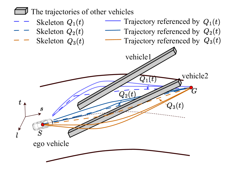
(a) Illustration of overtaking trajectory generation in the $s$-$l$-$t$ configuration space

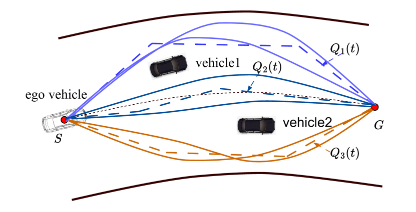
(b) Illustration of overtaking trajectory generation on the plane

Figure 2: Illustration of overtaking trajectory generation on the road. (a) Dashed lines represent trajectory skeletons from the upper-layer planner. Blue, purple and brown dashed lines belong to different topological classes. The solid lines show polynomial trajectories generated by the lower-layer planner, fitting based on the corresponding trajectory skeletons. Trajectories of the same color belong to the same topological class. (b) Distinctive topological trajectory represents a unique overtaking maneuver.

The initial state is denoted by $\mathcal{R}(0)$, the bounded input is $\mathcal{U}$. For the initial state $\xi(0)=\xi_{0},t\in[0,t_{f}]$, and trajectory $\mathcal{T}(\cdot)$, the state in reachable set is denoted by $\mathcal{X}(t,x_{0},\mathcal{T}(\cdot),u(\cdot))$. The exact reachable set for a reference trajectory $\mathcal{T}^{\star}(\cdot)$ is

$$\begin{split}\mathcal{R}^{e}([0,t_{f}])=&\bigg{\{}\mathcal{X}(t,\xi_{0},\mathcal{T}(\cdot),u(\cdot))\big{|}t\in[0,t_{f}],\\ &\xi_{0}\in\mathcal{R}(0),\mathcal{T}(t)=\mathcal{T}^{\star}(t),u(t)\in\mathcal{U}\bigg{\}}\end{split}$$ (1)

Combine the state and input vector to a new vector $z=[\xi,u]$. For simplicity, using a first-order Taylor expansion around the linearization point $z^{\star}=[\xi^{\star},u^{\star}]$, for $\forall t\in[\tau_{k},\tau_{k+1}]$

$$\dot{\xi}_{i}\in f(z^{\star})+\frac{\partial f}{\partial z}\bigg{|}_{z=z^{\star}}\oplus\mathcal{L}_{i}(\tau_{k})$$ (2)

$$\frac{\partial f}{\partial z}\bigg{|}_{z=z^{\star}}(z-z^{\star})=\frac{\partial f}{\partial\xi}\bigg{|}_{\xi=\xi^{\star}}(\xi-\xi^{\star})+\frac{\partial f}{\partial u}\bigg{|}_{u=u^{\star}}(u-u^{\star})$$ (3)

where $\oplus$ represents set-based addition [30], $\mathcal{L}$ is the set of Lagrange remainders:

$$\begin{split}\mathcal{L}_{i}(\tau_{k})=&\bigg{\{}\frac{1}{2}(z-z^{\star})^{T}\frac{\partial^{2}f}{\partial z^{2}}\bigg{|}_{z=z^{\star}}(z-z^{\star})\\ &\bigg{|}(\eta=\mathcal{R}(\tau_{k})\times\mathcal{U},z=\mathcal{R}(\tau_{k})\times\mathcal{U})\bigg{\}}\end{split}$$ (4)

Starting from $\mathcal{R}(t_{k})$, compute the set of all solutions $\mathcal{R}_{h}(t_{k}+1)$ for the linearized system $\dot{\xi}=A\xi+Bu$. Using $r=t_{k+1}-t_{k}$, the solution of $\mathcal{R}_{h}(t_{k+1})$ is as follows:

$$\begin{split}\mathcal{R}_{h}^{d}(t_{k+1})&=e^{Ar}\mathcal{R}(t_{k})+x_{p}(r)\\ &=e^{Ar}\mathcal{R}(t_{k})+\int_{0}^{\tau}e^{A(r-t)}dtu_{c}\end{split}$$ (5)

An interval matrix $\epsilon_{p}(r)=[-W(r)r,W(r)r]$ is introduced in [36], then the particular solution $x_{p}(r)$ is bounded by

$$\begin{split}x_{p}(r)\in\Gamma(r)\otimes u_{c}\end{split}$$ (6)

where $\otimes$ represents set-based multiplication [30], $\Gamma(r)$ is as follows:

$$\begin{split}\Gamma(r)=\sum_{i=0}^{\gamma}\frac{A^{i}r^{i+1}}{(i+1)!}\oplus\epsilon_{p}(r)\end{split}$$ (7)

Considering the uncertainty of input $U_{r}$, the reachable set is

$$\begin{split}\mathcal{R}_{p}(r)=\bigg{[}\sum_{i=0}^{\gamma}\frac{A^{i}r^{i+1}}{(i+1)!}\otimes U_{r}\bigg{]}\oplus\bigg{[}\epsilon_{p}(r)\otimes\left|U_{r}\right|\bigg{]}\end{split}$$ (8)

The enlargement required to bound all affine solutions within $\tau_{k}$ is denoted by $\mathcal{R}_{\epsilon}$ The reachable set for the next point in time and time interval is obtained by combining all previous results and using the operator $co(\cdot)$ for the convex hull:

$$\mathcal{R}(t_{k+1})=e^{Ar}\mathcal{R}(t_{k})\oplus\Gamma(r)u_{c}$$ (9a)

$$\mathcal{R}(\tau_{k})=co(\mathcal{R}(t_{k}),\mathcal{R}(t_{k+1}))\oplus\mathcal{R}_{\epsilon}\oplus\mathcal{R}_{p}(r)$$ (9b)

Based on the above method, the reachable set of the vehicle system at any given time can be calculated given the initial state and control inputs.

4 The Overtaking Trajectory Planning Framework

In this chapter, the implementation details of the overtaking trajectory planning framework based on spatio-temporal topology and reachable set analysis are introduced. The overall structure of the algorithm is shown in Figure 1.

4.1 Overall Framework

The overtaking trajectory planning framework includes the upper-layer planner based on spatiotemporal topological search method (STS). And the lower-layer planner based on parallel trajectory generation using reachable sets (RPTG). The upper-layer planner translates the trajectories of other vehicles on the road into the $s$-$l$-$t$ configuration space, treating them as static obstacles. It performs sampling in the $s$-$l$-$t$ configuration space and applies graph search methods to identify a set of collision-free initial trajectories from different topological classes. The lower-layer planner concurrently optimizes these initial trajectories to derive time-parameterized polynomial candidate trajectories. Leveraging the differential flatness property of the vehicle, the inputs of can be determined at specific time instances. The reachable sets method is then used to assess the control feasibility of the candidate trajectories. The optimal collision-free and highly control-feasible trajectory is selected as the overtaking trajectory, which is provided to the controller for tracking.

4.2 Spatio-temporal Topological Search Method

In the spatio-temporal configuration space, the trajectory of other moving vehicles is regarded as a static obstacle, dividing the entire search space into independent topologies. This section aims to search within these topological spaces to obtain a series of trajectory skeletons that represent different motion behaviors, providing references for subsequent trajectory generation.

4.2.1 Notation Description

As shown in Fig.3, the spatio-temporal sampling space consists of the plane and time, the sampling node $p=\mathbb{R}^{2}\times[0,T]$. The trajectory of $j$th vehicles is regarded as an obstacle, $j\in\mathbb{N}_{0}$, the occupancy states set is represented by the thick black lines. In this section, the Frenet coordinate system [37] is constructed along the road centerline. Table 1 explains some symbols in this section.

  Algorithm 1 Spatio-temporal Graph Construction

 

1:  Input: $\mathbf{E}$:road map,$N_{s}$: maximum sample number, $N_{p}$: number of skeletons

2:  Output: $\mathcal{E_{r}}$: set of skeletons

3:  $\mathcal{E_{r}}\leftarrow\emptyset,N_{s}\leftarrow 0,N\leftarrow(p_{g}.s-p_{s}.s)/\Delta s,i\leftarrow 0$

4:  for each $layer_{i}$ do

5:     sample $N_{s}$ nodes and add them to $\mathcal{C}_{i}$

6:     for each $p_{1}\in layer_{i}$ do

7:        for each $p_{2}\in layer_{i+1}$ do

8:           if $\lnot$ LineVisbible($p_{1},p_{2}$) then

9:              find the first feasible link node $p_{l}$ in $\mathcal{C}_{i}$

10:              $p_{1}.E_{2},p_{2}.E_{1}\overset{+}{\leftarrow}\{p_{1},p_{l},p_{2}\}$

11:           else

12:              if IsReachable($p_{1},p_{1}$) then

13:                 $p_{1}.E_{2},p_{2}.E_{1}\overset{+}{\leftarrow}\{p_{1},p_{2}\}$

14:           UpdateSkeletonsCost($p_{1}$)

15:  Add all elements of $p_{g}.E$ to the priority queue $pq$

16:  $\mathcal{E_{r}}\leftarrow$ ExtractDistinctSkeletons($pq,N_{p}$)

17:  return  $\mathcal{E_{r}}$

 

The search graph shown in Fig.3 contains two types of sampling nodes: the $layer$ $node$ and $link$ $node$. The position of the $layer$ $node$ is obtained by sampling on the corresponding layer. Several link nodes are sampled in the free area between adjacent layers. When obstacles block the connections between the adjacent layers nodes, they can be bypassed using link nodes located between them, as indicated by the yellow edges, which is indicated in Fig.3. It is worth noting that $p_{g}$ contains a series of nodes with the exact geographic coordinates but differ in arrival times. Starting at node $p$, they backtrack through $p.E_{2}$ and $p.E_{1}$, recording each layer node and link node traversed until reaching $p_{s}$. This process constructs a trajectory skeleton $e$ from $p_{s}$ to $p$.

4.3 Search Referece Topological Skeletons

To extract candidate reference trajectory skeletons, traverse from the first layer, sampling a series of link nodes in the free space between every two adjacent layers. Traverse all nodes in the layer, attempting to connect with nodes in the next layer. Nodes within the same layer are not allowed to connect. If the line between two layer nodes is unobstructed and meets the maximum speed limit, these nodes can form an edge. If an obstacle obstructs the line between two nodes, find a suitable link node in the corresponding set $\mathcal{C}$ and connect it to aforementioned two-layer nodes. These three nodes form an edge if they are not obstructed and meet the maximum speed limit. Add the newly generated edge to the edges set of the corresponding layer nodes, then update the cost of each skeleton. Repeat the above process until all the edge sets of $p_{g}$ are updated. Add all skeletons from $p_{s}$ to $p_{g}$ to the priority queue according to cost in ascending order. Finally, skeletons with the lowest costs, each belonging to a different topological class, are extracted from the priority queue. The general structure is outlined in Algorithm 4.2.1.

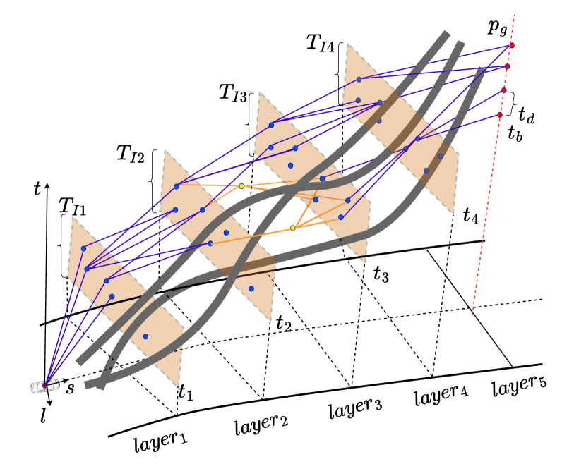
(a) Road search graph in spatio-temporal space.

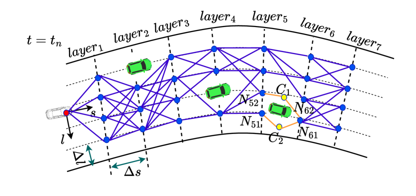
(b) The search space on raod at $t=t_{n}$.

Figure 3: Road skeleton search graph. In (a), the red nodes represent the start and end nodes. The blue nodes are layer nodes, and the yellow nodes are link nodes. The sampling time interval for $layer_{i}$ is $[t_{i},t_{i}+T_{Ii}]$. The brown boxes indicate the sampling range for each $layer_{i}$. The blue edges represent direct connections between layer nodes from adjacent layers. In (b), due to obstacles blocking the connections, it forms new edges:$\{p_{51},p_{l1},p_{61}\},\{p_{52},p_{l2},p_{62}\}$.

The distance between $p_{1}$ and $p_{2}$ is estimated by (10), denoted by $dist(p_{1},p_{2})$.

$$dist(p_{1}.p_{2})=\sqrt{(p_{2}.s-p_{1}.s)^{2}+(p_{2}.l-p_{1}.l)^{2}}$$ (10)

IsReachable($p_{1},p_{2}$) is used to determine whether $(p_{1},p_{2})$ is reachable. $(p_{1},p_{2})$ is reachable when $p_{2}.t-p_{1}.t\geq dist(p_{1},p_{2})/v_{m}$. This indicates that $p_{2}$ from $p_{1}$ can be reached without exceeding the maximum velocity $v_{m}$.

If the line between $p_{1}$ and $p_{2}$ is blocked by an obstacle, traverse the elements in $\mathcal{C}_{i}$ until a link node $p_{l}$ is found such that the line between $p_{1}$ and $p_{l}$, and the line between $p_{l}$ and $p_{2}$ both are unobstructed and are reachable.

The calculation of the cost of skeletons will be described in detail later. After adding all the skeletons from $p_{s}$ and $p_{g}$ to the priority queue $pq$, only a small number $N_{p}$ of skeletons with the smallest costs and different topologies are selected from $pq$ as reference skeletons. Uniform visibility deformation(UVD) proposed in [18] is used to determine the topological equivalence of the two skeletons in this section, as shown in Fig.4.

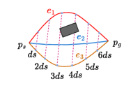
(a)

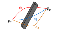
(b)

Figure 4: Skeletons topology equivalence. (a) Starting from $p_{s}$, a point is sampled every $ds$. If the line connecting the corresponding points is obstructed, it indicates that the two skeletons are topologically non-equivalent. (b) An illustration of topology equivalence, $e_{2}$ and $e_{3}$ are topological equivalents while the topology of $e_{1}$ is distinct to $e_{2}$ and $e_{3}$.

4.3.1 Cost Fucntion

The cost of the trajectory skeleton is calculated in the function UpdateSkeletonsCost, as shown in equation (11).

$$J_{\mathcal{E}}=c_{1}J_{T}+c_{2}J_{\theta}+c_{3}J_{len}+c_{4}J_{acc}+c_{5}J_{obs}$$ (11)

where $J_{T}$ represents the time cost of reaching the endpoint along the trajectory skeleton, $J_{\theta}$ represents the curvature cost of the path skeleton, $J_{acc}$ represents the acceleration cost of the skeleton, $J_{len}$ represents the length cost of the skeleton, and $J_{obs}$ represents the proximity cost of the path to obstacles. For the skeleton $\mathcal{E}$, which contains $N+1$ nodes, $p_{0}$ and $p_{N+1}$ are the starting and ending nodes of the skeleton, respectively. The specific calculation method for evaluating the cost of skeleton $\mathcal{E}$ is as follows:

$$t_{ref}=\frac{dist(p_{0},p_{N+1})}{v_{m}}$$ (12)

$$J_{T}\quad=\frac{p_{e}t}{t_{ref}}$$ (13)

$$J_{len}=\sum_{i=1}^{N}\frac{\lVert\overrightarrow{p_{i-1}p_{i}}\rVert}{dist(p_{0},p_{N+1})}$$ (14)

(13) and (14) calculate the time cost and length cost of the skeleton, respectively. (15) calculates angles between any three consecutive nodes $p_{i-1},p_{i},p_{i+1}$ by computing the angle formed between the vectors $\overrightarrow{p_{i-1}p_{i}}$ and $\overrightarrow{p_{i}p_{i+1}}$.

$$\theta_{i}=\arccos(\frac{\overrightarrow{p_{i-1}p_{i}}\cdot\overrightarrow{p_{i}p_{i+1}}}{\lVert\overrightarrow{p_{i-1}p_{i}}\rVert\cdot\lVert\overrightarrow{p_{i}p_{i+1}}\rVert})$$ (15)

$$J_{\theta}=\sum_{i=1}^{N}\frac{\theta_{i}}{\pi}$$ (16)

This paper explores using standard deviation analysis on a series of acceleration measurements to assess the stability of acceleration variation. A smaller standard deviation indicates smoother changes in acceleration, which may correlate with higher comfort levels. $\Delta t_{i-1}$ represents the time deviation between $p_{i}$ and $p_{i-1}$ while $\Delta t_{i}$ represents the time deviation between $p_{i+1}$ and $p_{i}$. The average acceleration across all points is denoted as $\bar{a}$, $a_{i}$ is the acceleration at node $p_{i}$.

$$a_{i}=\frac{2(\lVert\overrightarrow{p_{i}p_{i+1}}\rVert/\Delta t_{i}-\lVert\overrightarrow{p_{i-1}p_{i}}\rVert/\Delta t_{i-1})}{(\Delta t_{i-1}+\Delta t_{i})}$$ (17)

$$J_{acc}=\sqrt{\frac{1}{N}\sum_{i=1}^{N}(a_{i}-\bar{a})^{2}}$$ (18)

As defined in Equation (19), a penalty function is used to penalize points on the trajectory that come too close to obstacles. Points located within a threshold distance $r_{th}$ from obstacles are subject to a penalty that increases as the distance decreases. This penalty function encourages trajectories to maintain a safe distance from obstacles. A total of $M$ points are sampled uniformly along the skeleton.

$$J_{obs}=\sum_{i=1}^{M}\frac{(r_{th}-\min(r_{th},r_{i}))}{M\cdot r_{t}h}$$ (19)

In this section, a series of topological reference trajectories are generated in the $s$-$l$-$t$ configuration space. These topological reference trajectories, belonging to different topological classes, represent independent motion behaviors. Therefore, optimizing these reference skeletons as initial solutions can help avoid getting trapped in local optima, thereby improving the quality of the resulting trajectories. The lower-layer trajectory planner utilizes these topological reference skeletons as initial solutions and generates a set of collision-free candidate trajectories in parallel. The specific implementation details of the lower-layer trajectory planner will be discussed in the next section.

4.4 Parallel Trajectory Generation Method Based on Reachable Set

This section outlines a method for generating parallel feasible trajectories using reachable sets. The process begins by obtaining a series of reference skeletons from different topological classes. Then, the lower-layer trajectory planner optimizes each reference skeleton in parallel, ultimately selecting the optimal, control-feasible trajectory for overtaking. Initially, each reference skeleton is fitted using a quintic polynomial. The fitting problem is formulated as a quadratic programming problem, considering both the fitting cost of the quintic curve to the skeleton and the jerk cost of the curve. By adjusting the ratio between these two costs, a set of candidate fitting trajectories can be generated in parallel. Although these trajectories can be efficiently obtained through quadratic programming, this approach does not consider the kinematic model of the vehicle, and thus cannot guarantee control feasibility. To address this issue, the necessary inputs for the candidate trajectories are computed based on the differential flatness property. Finally, using these inputs, reachable sets are employed to identify the optimal, control-feasible trajectory from among the candidate curves, resulting in the final overtaking trajectory.

4.4.1 Candidate Trajectories Generation

The trajectory skeletons generated in Section 4.2 will be fitted with polynomials to create a series of candidate trajectories in this section. These candidate trajectories will later be evaluated for collision-free status and control feasibility. The position of the vehicle can be described by a polynomial with degree $n$, $Q(t)=\mathbf{k}^{T}\beta(t)$, $t\in[0,T]$ where the coefficient vector $\mathbf{k}\in\mathbb{R}^{2n}$, $T$ is the time duration, $\beta(t)=(1,t,t^{2},\cdots,t^{2n-1})^{T}$ is the natural basis. $Q^{\star}(t)$ is the trajectory skeleton. The above trajectory fitting problem can be formulated as an optimization problem in the following form:

$$\begin{split}&\min\,\,J\\ &s.t.\quad\begin{array}[]{lc}Q^{(j)}(T)=Q^{\star(j)}(T)\\ Q^{(j)}(0)=Q^{\star(j)}(0),j\in\{0,1,2\}\end{array}\end{split}$$ (20)

where the constraints include position, velocity and acceleration constraints at the start and goal. The form of the objective function in (20) is as follows.

$$J=\sum_{i=0}^{m-1}{\alpha_{1}\int_{0}^{T}\left\|Q(t)-Q^{\star}(t)\right\|^{2}dt}+{\alpha_{2}\int_{0}^{T}\left\|\dddot{Q}(t)\right\|^{2}dt}$$ (21)

(21) consists of two parts: the first part is the cost of deviation between the polynomial trajectory and the skeleton, and the second part is the cost of the smoothness of the polynomial trajectory. Since the optimization problem only includes equality constraints, it can be rewritten as an unconstrained quadratic optimization problem, which can be solved fast [38].

Since the original trajectory skeleton $Q^{\star}$ is collision-free, increasing $a_{1}$ makes the polynomial trajectory closer to $Q^{\star}$. However, this sacrifices smoothness and might make the trajectory infeasible. On the other hand, increasing $a_{2}$ results in a smoother polynomial trajectory, but it deviates further from $Q^{\star}$, potentially causing collisions. To determine the best combination of $a_{1}$ and $a_{2}$, this paper explores various pairs of $a_{1}$ and $a_{2}$, generating multiple candidate trajectories for each skeleton. These trajectories are then evaluated for collision status and control feasibility to determine the optimal trajectory.

4.4.2 Determine the Inputs Based on Differential Flatness

To evaluate the control feasibility of candidate trajectories, it is first necessary to determine the states and inputs of the vehicle along the trajectories. From the differential flatness property of the vehicle, it is known that the states and inputs can be derived from the position and their finite-order derivatives [39]. This section will illustrate deriving the states and controls from the polynomial trajectories.

For the kinematic bicycle model in Cartesian coordinates frame, the state vector $\mathbf{\xi}=(x,y,v,\theta)^{T}$, the input vector $\mathbf{u}=(a_{t},\delta)^{T}$. Where $(x,y)^{T}$ is the position at the center of the rear wheels, $v$ is the longitudinal velocity, $a_{t}$ is the longitude acceleration, and $\delta$ is the steering angle. Based on the characteristics of differential flatness, all information is expressed through $(x,y)^{T}$, as shown in equation (22d).

$$v=\sqrt{\dot{x}^{2}+\dot{y}^{2}}$$ (22a)

$$\theta=\tan^{-1}(\dot{y}/\dot{x})$$ (22b)

$$a_{t}=(\dot{x}\ddot{x}+\dot{y}\ddot{y})/\sqrt{\dot{x}^{2}+\dot{y}^{2}}$$ (22c)

$$\delta=\tan^{-1}((\dot{x}\ddot{y}-\dot{y}\ddot{x})L/(\dot{x}^{2}+\dot{y}^{2})^{\frac{3}{2}})$$ (22d)

where $L$ is the length of the wheelbase. Thus, the flat outputs $(x,y)^{T}$ and their finite derivatives describe the arbitrary state and input information of the vehicle.

4.4.3 Evaluate Control Feasibility Using Reachable Sets

After obtaining the states and inputs of the ego car along the candidate trajectories, this section introduces the reachable sets to evaluate the control feasibility of the candidate trajectories in parallel. A continuous state space representation of the kinematic vehicle model can be expressed as:

$$\dot{\xi}=f(\xi,u)\equiv \dot{x}=\cos(\theta)\cdot v$$ (23a)

$$\dot{\xi}=f(\xi,u)\equiv \dot{y}=\sin(\theta)\cdot v$$ (23b)

$$\dot{\xi}=f(\xi,u)\equiv \dot{\theta}=\tan(\delta)/L\cdot v$$ (23c)

$$\dot{\xi}=f(\xi,u)\equiv \dot{v}=a_{t}$$ (23d)

According to the calculation of reachable sets described in section 3, the kinematic model in (23d) is first linearized as follows:

$$f(\xi,u)\cong f(\xi^{\star},u^{\star})+\frac{\partial f}{\partial\xi}\bigg{|}_{\xi=\xi^{\star}}(\xi-\xi^{\star})+\frac{\partial f}{\partial u}\bigg{|}_{u=u^{\star}}(u-u^{\star})$$ (24)

$$\xi_{k+1}=\xi_{k}+f(\xi_{k},u_{k})\cdot dt$$ (25)

Convert the above formula into matrix form.

$$\xi_{k+1}=A_{k}\xi_{k}+B_{k}u_{k}$$ (26)

$$A_{k}=\begin{bmatrix}A_{k}^{\star}&C_{k}^{\star}\\ \mathbf{0}&\mathbf{0}\end{bmatrix}\quad B_{k}=\begin{bmatrix}B_{k}^{\star}\\ \mathbf{0}\end{bmatrix}$$ (27)

$$A_{k}^{\star}=\frac{\partial f}{\partial\xi}\bigg{|}_{\xi=\xi^{\star}}\cdot dt$$ (28)

$$B_{k}^{\star}=\frac{\partial f}{\partial u}\bigg{|}_{u=u^{\star}}\cdot dt$$ (29)

$$C_{k}^{\star}=f(\xi^{\star},u^{\star})\cdot dt-A_{k}^{\star}\xi^{\star}-B_{k}^{\star}u_{k}^{\star}$$ (30)

where $\xi_{k}=\begin{bmatrix}\xi&\mathbf{I}\end{bmatrix}^{T}$. $\mathbf{0}$ and $\mathbf{I}$ are the zero matrix and identity matrix with appropriate dimensions.

The planning time horizon is the arriving time $T$ of the goal. The time increment is $\Delta T$, $T=N\Delta T$. A discrete step is denoted by $k\in\mathbb{N}_{0}$ , $k\in[0,N]$. The discrete-time at $k$, $t_{k}=k\Delta T$. Then the corresponding linearized model is obtained based on (25)-(27) at each $t_{k}$. Starting from $t=0$, a linearized reference state $\xi^{\star}_{k}$ is selected on the candidate trajectory at intervals of $\Delta T$. From all states in $\mathcal{R}_{k}$, the system is simulated forward for a time interval $\Delta T$ using the linearized model at $\xi_{k}$, under the bounded inputs and the input uncertainty $U_{r}$. Thus the next reachable set $\mathcal{R}_{k+1}$ is then calculated by (9b). The initial reachable set $\mathcal{R}_{0}$ contains only one state $\xi_{0}$. This process repeats until the reachable set at the final time $T$ is determined. To describe a trajectory with high control feasibility, the following definition is provided.

Definition 1 (High Control Feasibility Trajectory)

Given the trajectory $\mathcal{T}(x,u)$ with the initial state $\xi_{0}^{\star}$ at time $t_{0}$. The linearization horizon is $N$, the linearization state of the trajectory is $\xi_{k}^{\star}$ at time $t_{k}$. The consecutive time intervals $\tau_{k}=[t_{k},t_{k+1}]$, $\mathcal{T}(x,u)$ is regarded as kinematic feasible trajectory in $[t_{0},t_{k+1}]$ if $\xi_{k}\in\mathcal{R}(\tau_{k})$, $\forall k\in N$.

Since it is impossible to enumerate the reachable sets at all times, the high control feasibility of the candidate trajectories is approximately determined according to the method in Definition 1. Figure 5 provides intuitive examples of trajectories with high control feasibility and those with low control feasibility, respectively.

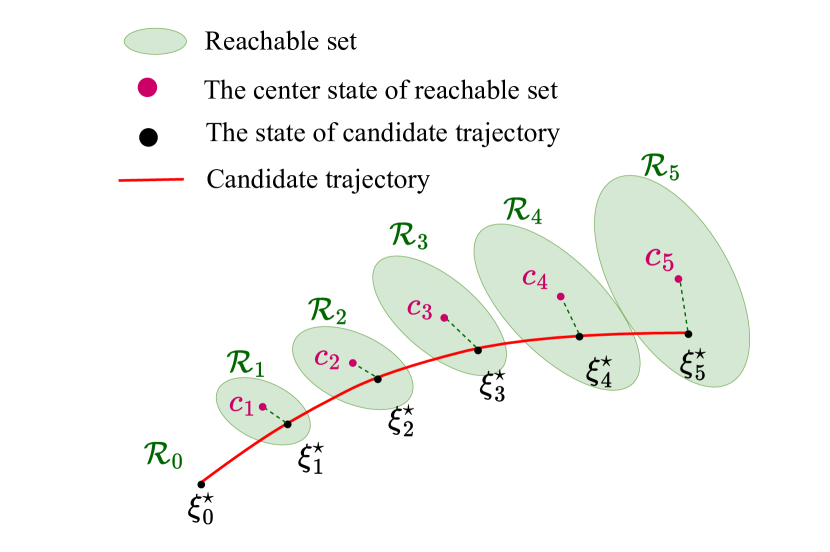
(a)

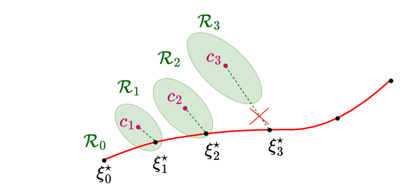
(b)

Figure 5: Illustration of using reachable sets to determine trajectory control feasibility. (a) $\mathcal{R}_{0}$ is the reachable set of the vehicle at $t=0$, and it is a single state. Along the trajectory, linearized reference states, such as $\xi^{\star}_{0}$-$\xi^{\star}_{5}$, are determined at intervals of $\Delta T$. In the diagram, each state is contained within its corresponding reachable set, indicating that the trajectory has high control feasibility. (b) This diagram shows a low control feasibility trajectory because $\xi^{\star}_{3}$ is no longer contained within its corresponding reachable set.

There may be multiple trajectories with high control feasibility, so it is necessary to select the optimal trajectory as the overtaking trajectory. Therefore, the control feasibility of the trajectories is evaluated according to the following aspects:

$$J_{RS} =J_{p}+J_{v}+J_{\theta}$$

$$=\frac{1}{N}\sum_{i=1}^{N}\left(\lambda_{1}\frac{p^{d}_{k}}{d_{r}}+\lambda_{2}\frac{v^{d}_{k}}{v_{r}}+\lambda_{3}\frac{\xi^{d}_{k}}{\theta_{r}}\right)$$ (31)

where $J_{p}$ represents the average deviation cost of the trajectory points from the center of the corresponding reachable set in position; $J_{v}$ represents the average deviation cost of the trajectory states from the center of the corresponding reachable set in velocity; and $J_{\theta}$ represents the average deviation cost of the trajectory states from the center of the corresponding reachable set in heading angle. $p^{d}_{k}$, $v^{d}_{k}$, and $\theta^{d}_{k}$ represent the position deviation, velocity deviation, and orientation angle deviation between the reference state $\xi^{\star}_{k}$ and the center $c_{k}$ of the corresponding reachable set, respectively. $\lambda_{1}$, $\lambda_{2}$, and $\lambda_{3}$ are coefficients, and $d_{r}$, $v_{r}$, and $\theta_{r}$ are reference values used to normalize the corresponding terms. Specifically,

$$p^{d}_{k}=\sqrt{(c_{k}.x-\xi^{\star}_{k}.x)^{2}+(c_{k}.y-\xi^{\star}_{k}.y)^{2}}$$ (32)

$$v^{d}_{k}=\lvert c_{k}.v-\xi^{\star}_{k}.v\rvert$$ (33)

$$\theta^{d}_{k}=\lvert c_{k}.\theta-\xi^{\star}_{k}.\theta\rvert$$ (34)

The smaller the value of $J_{RS}$, the smaller the deviation between the reference state and the center of the reachable set, indicating stronger robustness and control feasibility. The trajectory corresponding to the smallest $J_{RS}$ will be selected as the overtaking trajectory.

5 Experimental Results and Discussion

In this section, we validate the proposed algorithm in simulation. To verify the performance and efficiency of the proposed method, we compared it with a common hierarchical planning approach, where the upper layer uses a breadth-first search (BFS) method [40], and the lower layer employs a Nonlinear Model Predictive Control (NMPC) [41] trajectory optimization method. The algorithm was implemented in C++/Python, and the CPU used for the experiments is an AMD Ryzen 7 5800H running at 3.2 GHz.

5.1 Simulation Setup

The vehicle kinematic parameters are shown in Table 2. The uncertainties in vehicle acceleration and front wheel angle arise from sensor uncertainties. To simplify the problem, we will assume these uncertainties to be constant values.

Table 2: Simulation parameter settings

Parameter	Description	Value
$v_{m}$	Maximum velocity	$15\,m/s$
$a_{m}$	Maximum acceleration	$5\,m/s^{2}$
$Length$	The length of car	4.3  m
$width$	The width of car	1.9  m
$L$	The wheelbase	2.8  m
$\delta_{m}$	Maximum steer angle	$\pi/6\,rad$
$r_{th}$	The safe distance	0.1 m
$U_{r}$	Input uncertainties	$[0.01\,m/s^{2},0.005\,rad]$

5.2 On the Effectiveness and Efficiency of Our Method

5.2.1 The effect of different fitting parameters on trajectory quality

In this section, we evaluate how fitting parameters affect the feasibility of the trajectory. Given a trajectory skeleton and under the uncertainty of the given control inputs, the lower-layer planner evaluates different polynomial trajectories in parallel and selects the optimal one as the final overtaking trajectory. The polynomial trajectories are generated by (21), where we fix $\alpha_{1}=1$ and vary the value of $\alpha_{2}$ 0 to 1.The fitting parameter scale factor $r_{\alpha}=\frac{\alpha_{2}}{\alpha_{1}}$. A smaller $r_{\alpha}$ indicates that the fitted trajectory is closer to the trajectory skeleton. As shown in Figure 6, the shapes of the fitting curves for these different values are displayed. Since the trajectory skeleton is guaranteed to be collision-free, the closer the trajectory is to the skeleton, the more likely it is to avoid collisions, but at the expense of reduced smoothness. Conversely, larger values of $r_{\alpha}$ result in higher smoothness for the trajectory, but they also lead to a greater deviation from the trajectory skeleton, which may increase the risk of collisions. Here are descriptions of several key metrics used to evaluate the trajectory:

• $\bm{len}$: the length of trajectory

• $\bm{T}$: the time to reach the trajectory endpoint.

• $\bm{d_{o,min}}$: the minimum distance between the trajectory and obstacles.

• $\bm{R_{o}}$: the portion of the trajectory where the distance to obstacles is less than $r_{th}$ relative to the entire trajectory.

• $\bm{J_{s}}$: the smoothness of the trajectory.

• $\bm{J_{\dot{\delta}}}$: the rate of change of the front wheel steering angle as the vehicle follows the trajectory.

Among the aforementioned metrics, $len$ and $T$ represent the efficiency of trajectory execution. $d_{o,min}$ and $R_{o}$ represent the safety of the trajectory. And $J_{s}$ and $J_{\dot{\delta}}$ represent the stability of the control inputs for the trajectory. We define an operator $IP(\cdot)$ that represents the percentage improvement of the current value relative to a reference value. For example, $IP(T)=\frac{T_{r}-T_{c}}{T_{r}}$, $IP(T)$ is the proportion by which the completion time $T_{c}$ of the current trajectory is reduced compared to the completion time $T_{r}$ of the reference trajectory.

The table 3 indicates that as the value of $r_{a}$ increases, the length of the generated trajectory decreases. In the case of $d_{o,min}$, it is evident that as $r_{a}$ increases, the distance between the trajectory and the obstacle tends to decrease. However, this relationship is not strictly monotonic, as it is influenced by the motion trajectory of vehicles. For instance, when $r_{a}=0.005$, the minimum distance between the autonomous vehicle and another vehicle is 0.439 meters. When $r_{a}$ exceeds 0.015, the trajectory collides with the other vehicle. According to $R_{o}$, when $r_{a}$ is less than 0.05, the minimum distance between the autonomous vehicle and the other vehicle exceeds $r_{th}$. However, when $r_{a}$ surpasses 0.025, the proportion of the trajectory length that falls below $r_{th}$ gradually increases with the rising value of $r_{a}$, eventually leading to collisions. The data from $d_{o,min}$ and $R_{o}$ suggest that when $r_{a}$ reaches a certain threshold, the deviation of the trajectory from the reference path increases, thereby raising the risk of collision with the other vehicle. This threshold is variable, depending on the driving states of both vehicles and the road environment. To tackle this issue, the lower-layer planner employing the RPTG method tests various $r_{a}$ values and generates trajectories in parallel for safety assessments. This approach enables the automatic selection of $r_{a}$ values that ensure trajectory safety in diverse scenarios.

A smaller $r_{a}$ indicates that the fitted trajectory is closer to the reference path, resulting in greater safety. However, a lower $r_{a}$ may also lead to reduced smoothness of the fitted trajectory. With $r_{a}=0$, the smoothness $J_{s}$ of the trajectory reaches 567.427 $m^{2}/s^{5}$, and as $r_{a}$ increases, the smoothness of the trajectory improves rapidly. When $r_{a}$ exceeds 0.05, there is more than a 90% reduction in smoothness compared to $r_{a}=0$. Similarly, as $r_{a}$ increases, the rate of change of the front wheel angle gradually decreases, indicating improved control stability of the trajectory. When $r_{a}=1$, the rate of change of the front wheel angle decreases by over 90% compared to $r_{a}=0$. In summary, the data demonstrate that a smaller $r_{a}$ results in higher safety for the trajectory, while a larger $r_{a}$ enhances smoothness and control stability. Considering these factors together can help identify an optimal trajectory, such as the one corresponding to $r_{a}=0.015$ in the scenario.

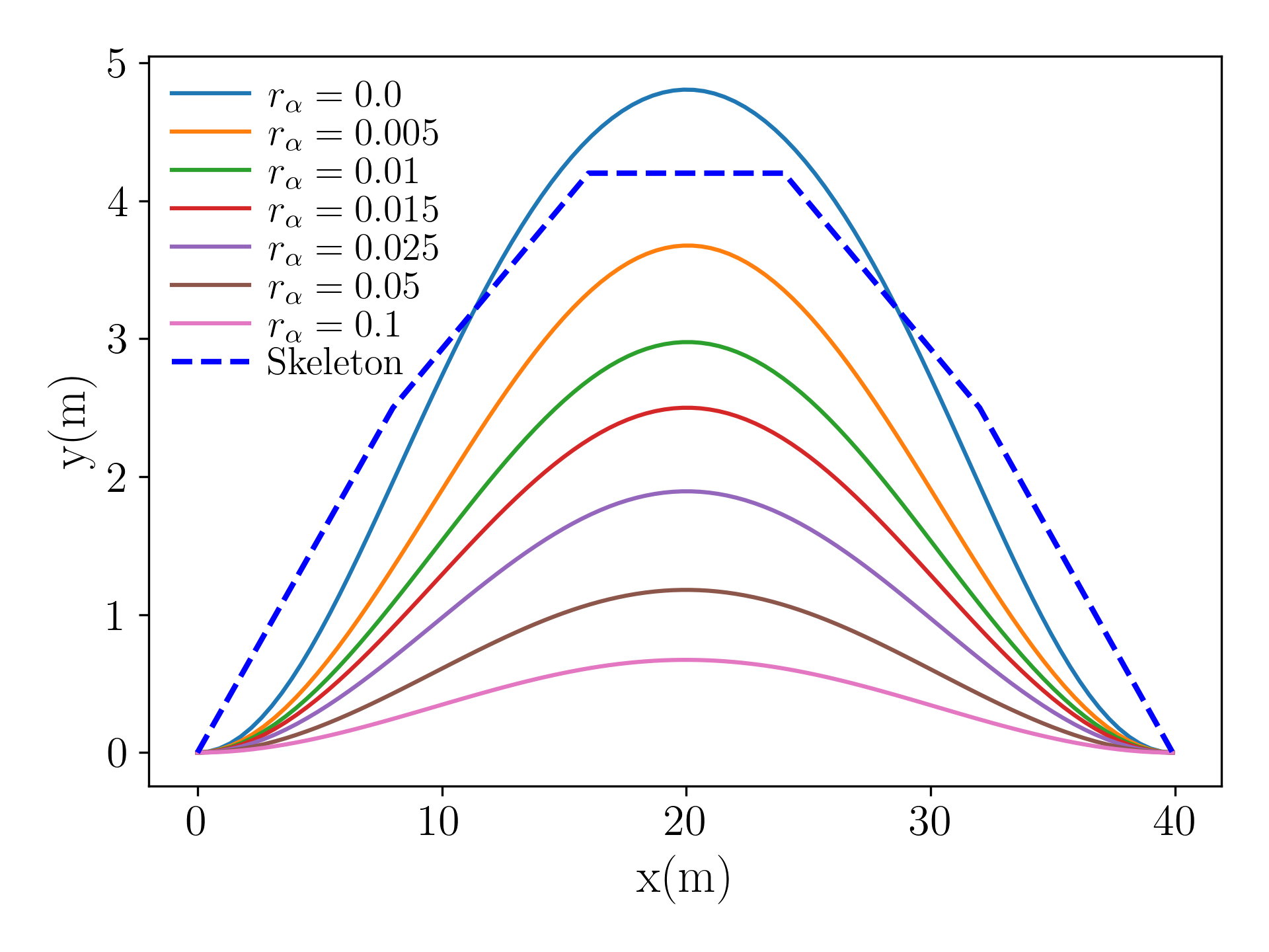
Figure 6: The candidate trajectories generated with different fitting parameters. The blue dashed line represents the trajectory skeleton, and the solid lines represent the candidate trajectories. The larger the value of $r_{\alpha}$, the greater the deviation of the candidate trajectories from the trajectory skeleton.

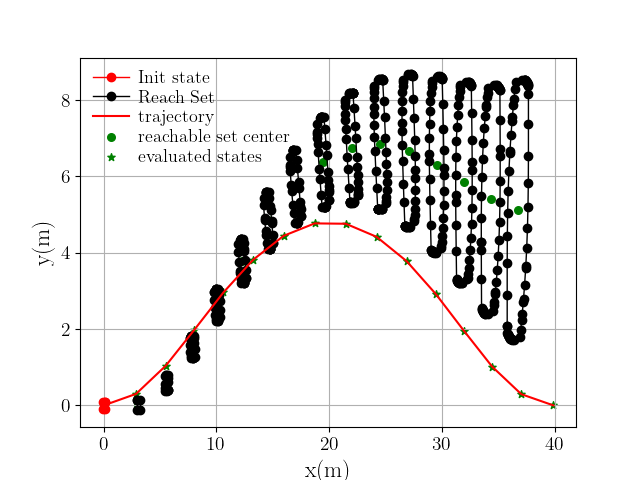
(a) The reachable sets corresponding to $r_{\alpha}=0.0$

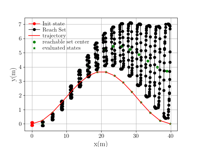
(b) The reachable sets corresponding to $r_{\alpha}=0.005$

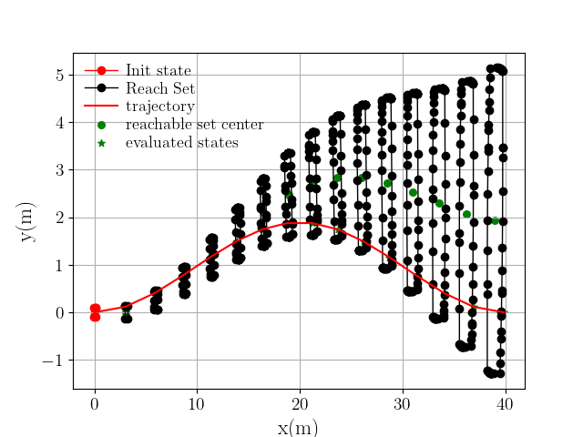
(c) The reachable sets corresponding to $r_{\alpha}=0.025$

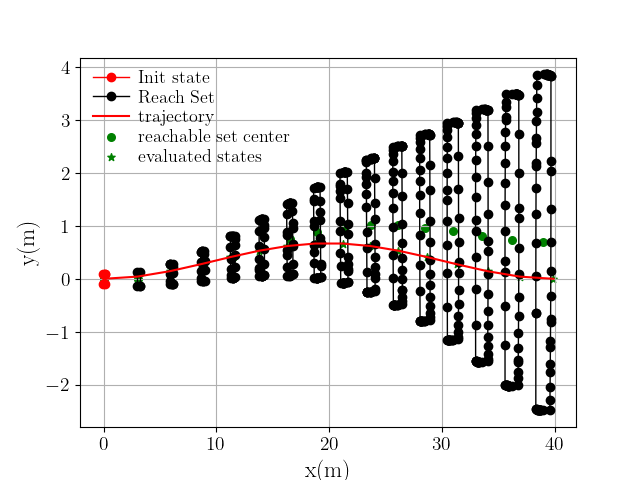
(d) The reachable sets corresponding to $r_{\alpha}=0.1$

Figure 7: The reachable sets corresponding to the trajectories with different fitting parameters. The red lines represent the fitted candidate trajectories. The green asterisks on the trajectories indicate states sampled from the trajectories at equal time intervals, $T/N_{RS}$. The black dots and lines forming the closed regions represent the reachable sets, which correspond to the green asterisks at the same time steps along the trajectories. The green dots indicate the centers of the corresponding reachable sets. From the figure, it can be observed that as $r_{\alpha}$ increases, the trajectories get closer to the centers of the reachable sets, indicating relatively high control feasibility. When the trajectory points fall outside the reachable sets, it implies that the control feasibility of the trajectories is relatively poor, such as in the case where $r_{\alpha}=0$.

The step size $N_{RS}$ for analyzing the reachable set of trajectories is set to 15. As shown in Figure 7, the larger the value of $r_{\alpha}$, the closer the overtaking trajectory is to the center of the reachable set, indicating higher feasibility of the trajectory. The metrics to describe the deviation of the trajectory from the reachable set are $J_{s}$, $J_{v}$, $J_{\theta}$ and their sum $J_{RS}$, which are shown in (31). As shown in Table 3, when $r_{\alpha}=0$, the trajectory exhibits poor control feasibility because certain parts of the trajectory are not within the corresponding reachable set. Thus they cannot be selected as an overtaking trajectory. When $r_{\alpha}=0.1$, the trajectory has a high level of control feasibility, but collisions occur, thus it cannot be used as an overtaking trajectory either. When $r_{\alpha}=0.015$, the trajectory is both controllable and collision-free. Based on the sum of $J_{s}$, $J_{v}$ and $J_{\theta}$ the trajectory with the smaller value is selected as the final overtaking trajectory.

Table 3: The various metrics of trajectories are generated by different fitting parameters. It indicates that the optimal trajectory is chosen based on a balance of control feasibility, trajectory quality, and safety. The optimal fitting parameters are $r_{\alpha}=0.015$.

Parameter	Col.1	Reachable metrics				Evaluation metrics
$r_{a}$		$J_{p}$	$J_{v}$	$J_{\theta}$	$J_{RS}$	$len(m)$	$d_{o,min}(m)$	$R_{o}$	$J_{s}(m^{2}/s^{5})$	$IP(J_{s})$	$J_{\dot{\delta}}(rad/s)$	$IP(J_{\dot{\delta}})$
0.0002	N	0.534	0.094	0.039	0.667	41.411	0.386	0%	567.427	-	10.711	-
0.005	N	0.338	0.030	0.028	0.396	40.814	0.439	0%	217.634	61.7%	8.980	16.2%
0.010	N	0.276	0.027	0.023	0.326	40.535	0.225	0%	143.803	74.7%	7.322	31.6%
0.015	N	0.235	0.026	0.019	0.280	40.379	0.331	0%	102.894	81.9%	6.169	42.4%
0.025	Y	0.183	0.025	0.015	0.223	40.218	0.000	23.6%	61.227	89.2%	4.687	56.2%
0.050	Y	0.124	0.025	0.009	0.158	40.158	0.000	44.2%	26.900	95.3%	2.925	72.7%
0.100	Y	0.085	0.025	0.005	0.115	40.075	0.000	78.5%	12.227	97.9%	1.669	84.4%

• Col. is used to indicate whether the trajectory collides with an obstacle. A value of N signifies no collision, while a value of
  Y indicates a collision has occurred.

• The data marked in blue are the baseline for the column, used to calculate the corresponding $IP(\cdot)$ of the metric.

•   represents various metrics of the selected overtaking trajectory. Bold indicates the best results under the same experimen-
  tal conditions. They appear in the following tables with the same interpretation as explained here.

In this subsection, we explore how different combinations of fitting parameters affect the feasibility of trajectories. Given the distribution of obstacles and the current state of the ego vehicle, it is challenging to pre-determine which combination of fitting parameters will ensure a high level of control feasibility while remaining collision-free. Thus, the parallel trajectory generation method based on the reachable set offers an efficient approach to identifying suitable fitting parameters. It systematically enumerates a range of fitting parameters and evaluates the associated trajectories for control feasibility and safety in parallel. In this way, the planner can filter out the optimal overtaking trajectory.

5.2.2 Evaluate the control feasibility of the trajectory using a pure pursuit controller

In this section, we evaluate the control feasibility of the trajectories generated by RPTG using a trajectory tracking controller. We employ the commonly used pure pursuit algorithm [42] for trajectory tracking. This algorithm establishes a geometric relationship based on the preview path, the current vehicle position, and the front wheel steering angle, enabling effective trajectory tracking control. We assess the control feasibility of the trajectory by analyzing the performance of the pure pursuit controller. Improved tracking performance indicates higher control feasibility for any given controller, while reduced tracking performance suggests lower control feasibility.

Table 4: pure pursiut controller parameter settings

Parameter	Description	Value
$L$	Look-ahead distance coefficient	$0.1$
$L_{fc}$	Look-ahead distance	$0.8\,m/s^{2}$
$K_{p}$	Speed P controller coefficient	5
$n$	the horizon of controller	50

Root Mean Square Error (RMSE) is used to measure the overall magnitude of an error across all time steps.

$$E=\sqrt{\frac{1}{n}\sum_{i=1}^{n}e_{i}^{2}}$$ (35)

where $E$ is the RMSE, $e_{i}$ is the tracking error (e.g., lateral, longitudinal, tracking or yaw error) at the $i-$th timestamp, and $n$ is the execution step of the controller. The relevant parameter settings of the pure pursuit controller are shown in Table 4. We will analyze the tracking performance based on the following metrics.

• $\bm{E_{l}}$: the RMSE of lateral error, which measures the perpendicular distance from the vehicle to the reference trajectory.

• $\bm{E_{p}}$: the RMSE of tracking deviation, which measures the Euclidean distance between the vehicle and the reference trajectory at each time step.

• $\bm{E_{\theta}}$: the RMSE of yaw error, which measures the difference in heading angle between the vehicle and the reference trajectory, normalized to lie within the range of $[-\pi,\pi]$

• $\bm{w_{m}}$: mean yaw rate of trajectory. This quantifies the rate of change of the yaw of vehicle over time.

The data in Table 5 indicates that as $J_{RS}$ decreases, the tracking performance of the trajectory significantly improves. For instance, when $r_{a}=0.025$, the lateral tracking error is reduced by 64.5% with $r_{a}=0.$, and the heading angle tracking error decreases by 64.5%. When $r_{a}=0.1$, the reduction in lateral tracking error reaches 53.6%, and the heading angle tracking error is reduced by 87.1%. This demonstrates that as $J_{RS}$ decreases, the geometric tracking error during trajectory tracking becomes smaller, indicating greater trackability of the trajectory. Additionally, compared to $r_{a}=0$, the reduction in angular velocity during trajectory tracking is 87.3% when $r_{a}=0.1$. This suggests that a lower $J_{RS}$ leads to smoother trajectory tracking control. Overall, the results show that smaller values of $J_{RS}$ correlate with better tracking performance by the controller, which includes reduced tracking errors and smoother control inputs. This reinforces the validity of using the reachable set to assess the control feasibility of the trajectory, as it aligns with the observed trends in tracking performance.

Table 5: The relationship between the control feasibility of the trajectory and tracking performance. It indicates that the higher the control feasibility, the better the trajectory tracking performance is.

Parameter	$J_{RS}$	Tracking metrics
$r_{a}$		$E_{l}(m)$	$IP(E_{l})$	$E_{p}$ ($m$)	$IP(E_{p})$	$E_{\theta}(rad)$	$IP(E_{\theta})$	$\omega_{m}(rad/s)$	$IP(\omega_{m})$
0.0001	0.534	0.124	-	0.181	-	0.186	-	0.606	-
0.005	0.338	0.084	32.3%	0.173	4.4%	0.124	33.3%	0.404	33.3%
0.010	0.276	0.068	45.2%	0.127	29.8%	0.102	45.2%	0.331	45.4%
0.015	0.235	0.058	53.2%	0.108	40.3%	0.087	53.2%	0.281	53.6%
0.025	0.183	0.044	64.5%	0.106	41.4%	0.066	64.5%	0.215	64.5%
0.050	0.124	0.028	77.4%	0.097	46.4%	0.042	77.4%	0.135	77.7%
0.100	0.085	0.016	87.1%	0.084	53.6%	0.024	87.1%	0.077	87.3%

• The data marked in blue are the baseline for the column, used to calculate the corresponding $IP(\cdot)$ of the metric.

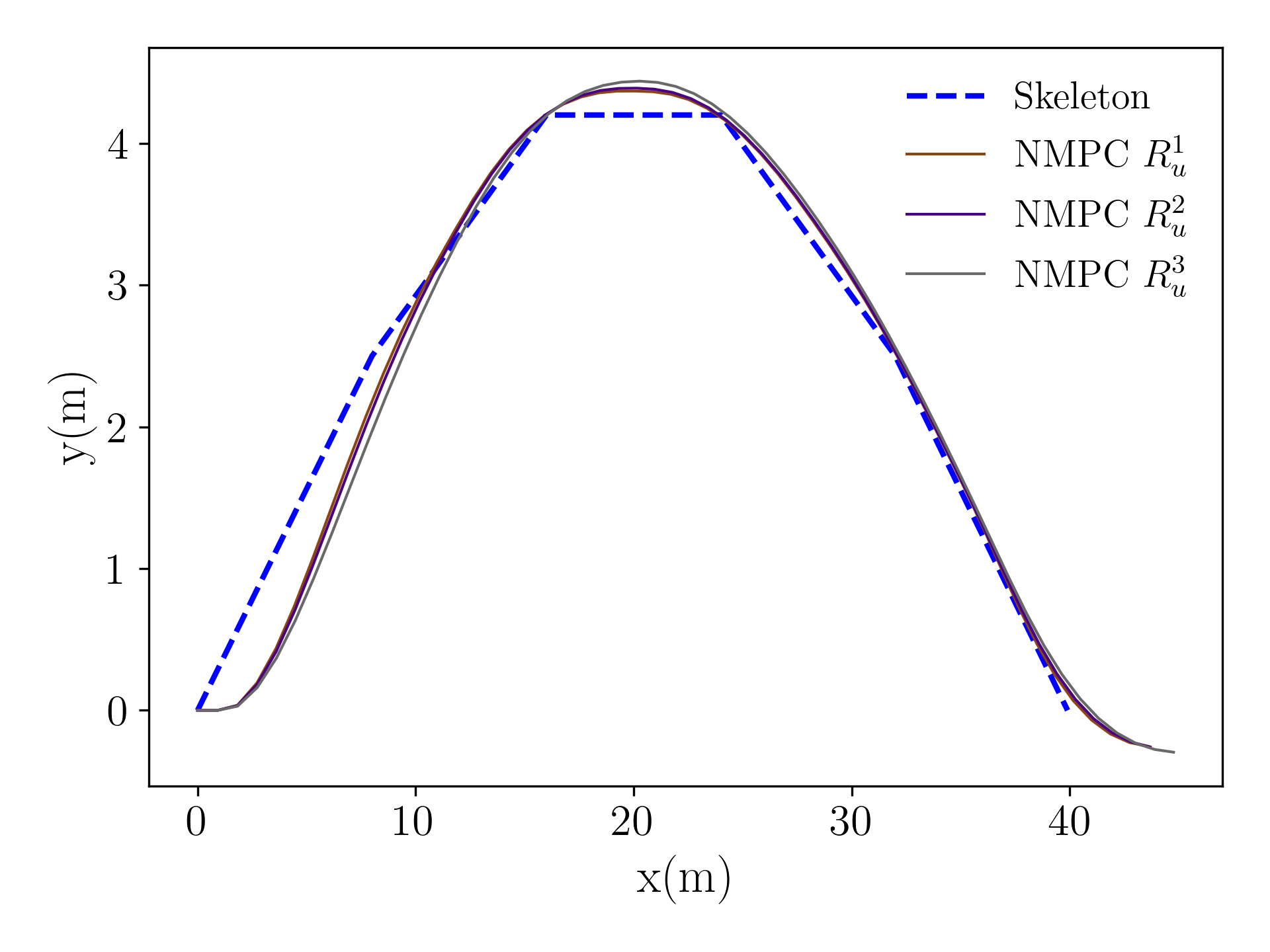
Figure 8: Comparison of the trajectory generated by NMPC. The position errors of NMPC trajectories show little variation across the different parameter settings compared to the trajectory skeleton.

5.2.3 Comparison of our lower-layer trajectory planner and the NMPC planner

Figure 9: Comparison of front wheel steering angles between trajectories generated by NMPC and RPTG. Compared to NMPC, the trajectory generated by RPTG has smaller front wheel steering inputs with less variability, indicating higher control stability.

In this section, we validate the effectiveness and efficiency of the proposed RPTG method by comparing it with numerical methods. Given the same trajectory skeleton, tests are conducted on both the lower-layer planner based on RPTG and the lower-layer planner based on NMPC. The basic form of the NMPC is as follows:

$$\min_{u} \sum_{k=0}^{N-1}\left(\xi_{k}^{\top}\mathbf{R_{s}}\xi_{k}+u_{k}^{\top}\mathbf{R_{u}}u_{k}\right)+\xi_{N}^{\top}\mathbf{R_{s}}\xi_{N}$$ (36)

s.t. $$\xi_{k+1}=f(\xi_{k},u_{k}),\quad k=0,1,\dots,N-1,$$

$$\xi_{0}=\xi_{\text{initial}},$$

$$u_{k}\in\mathcal{U},\quad\xi_{k}\in\mathcal{X},\quad k=0,1,\dots,N.$$

where $\xi_{init}$ represents the initial values of the state variables, $\mathcal{X}$ represents the set of feasible state values, and $\mathcal{U}$ represents the set of feasible control values. Here, the horizon is chosen as $N=15$. In the equations, $R_{s}$ represents the fitting cost coefficient to the skeleton, and $R_{u}$ represents the control input cost coefficient for the trajectory. We fix $R_{s}=diag([1.0,1.0,1.0,1.0])$ and provide three sets $R_{u}^{1}=diag([50.0,50.0]),R_{u}^{2}=diag([80.0,80.0]),R_{u}^{3}=diag([150.0,150.0])$ to evaluate the performance of NMPC. Testing has shown that a larger $R_{u}$ results in greater deviation between the trajectory and the skeleton, which can lead to collisions. Under the aforementioned settings, the trajectory generated by NMPC and the reference trajectory skeleton are shown in Figure 8.

As shown in the table 6, from the safety perspective, the NMPC method demonstrates better adherence to the topological reference skeleton, resulting in a greater minimum distance to obstacles compared to the RPTG method. Both methods maintain minimum distances that exceed the safe threshold distance $r_{th}$. Therefore, under the given parameter settings, the trajectories produced by both NMPC and RPTG meet the safety requirements. In terms of time efficiency, the RPTG method provides a significantly faster runtime, 61.6% less than NMPC. Regarding the smoothness metric, RPTG achieves a 73.7% improvement over the trajectories generated by NMPC. Figure 9 illustrates a comparison of the front wheel angles produced by both trajectory generation methods. The magnitude and variation of the front wheel angle in RPTG are smaller than those in NMPC, indicating that RPTG offers more excellent control stability. Overall, RPTG produces higher-quality trajectories compared to NMPC. Additionally, Since NMPC considers a nonlinear model, while RPTG decouples the vehicle model constraints from the optimization problem, the planning efficiency of the RPTG method is markedly superior than that of NMPC.

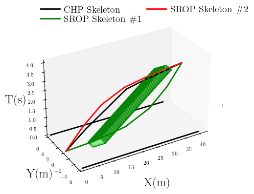
(a) The schematic diagram of overtaking scenario $S1$ in the $s$-$l$-$t$ coordinate system.

(b) The schematic diagram of overtaking scenario $S2$ in the $s$-$l$-$t$ coordinate system.

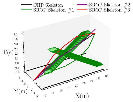
(c) The schematic diagram of overtaking scenario $S3$ in the $s$-$l$-$t$ coordinate system.

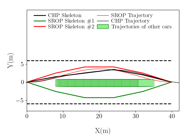
(d) The top-down view of overtaking trajectory in scenario $S1$.

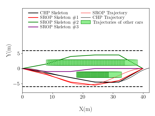
(e) The top-down view of overtaking trajectory in scenario $S2$.

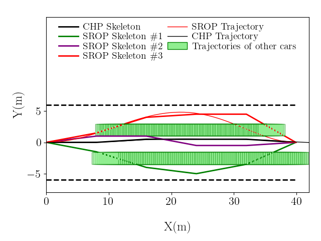
(f) The top-down view of overtaking trajectory in scenario $S3$.

Figure 10: (a), (b), and (c) are schematic diagrams of different overtaking scenarios in the $s$-$l$-$t$ coordinate system, while (d), (e), and (f) show the top-down views of the corresponding scenarios. The green cylinders represent the trajectories of other vehicles. The red, green, and purple polylines depict trajectory skeletons generated by SROP, each belonging to a different topological class, while the black polyline represents the trajectory skeleton planned by BFS. The red curve is the final overtaking trajectory fitted by SROP based on the corresponding skeleton, whereas the black curve represents the NMPC optimization of the BFS result. The dashed line indicates the ego vehicle reaching this position ahead of the other vehicle. From the figure, it can be observed that in scenario $S1$, the trajectory planned by SROP and the trajectory planned by CHP belong to the same topological class, whereas in scenarios $S2$ and $S3$, they belong to different topological classes.

Table 6: Compare the various metrics of the trajectories planned by the RPTG and NMPC. The results show that in terms of runtime and trajectory quality, RPTG outperforms NMPC.

Mehthod	Parameters	$J_{RS}$	Evaluation metrics
			$T_{r}(ms)$	$IP(T_{r})$	$len(m)$	$d_{o,min}(m)$	$v_{mean}$	$J_{\dot{\delta}}(rad/s)$	$IP(J_{\dot{\delta}})$
NMPC	$R_{u}=R_{u}^{1}$	-	192.311	-	43.911	1.594	13.815	27.621	-
	$R_{u}=R_{u}^{2}$	-	196.580	-	43.993	1.564	13.839	24.736	-
	$R_{u}=R_{u}^{3}$	-	187.262	-	45.063	1.535	13.906	20.167	-
NMPC avg1.	-	-	192.051	-	44.322	-	13.853	24.175	-
RPTG	$r_{a}=0.012$	0.306	71.864	62.6%	40.363	0.486	13.228	6.814	71.8%
	$r_{a}=0.014$	0.288	73.685	61.6%	40.304	0.364	13.209	6.370	73.7%
	$r_{a}=0.016$	0.273	75.923	60.5%	40.256	0.353	13.193	5.980	75.3%
RPTG avg.	-	-	73.824	61.6%	40.399	-	13.210	6.358	73.7%

• The data marked in blue are the baseline for the column, used to calculate the corresponding $IP(\cdot)$ of the metric.

5.2.4 Comparison of our SROP and other hierarchical planning method

In this subsection, we validate the effectiveness and high efficiency of the proposed hierarchical planning method, which is based on spatio-temporal topology and reachable set analysis. For comparison, we selected a commonly used hierarchical trajectory planning method (CHP). In CHP, the upper-layer planner uses a breadth-first search (BFS) algorithm to find a trajectory that minimizes length and time in the spatiotemporal graph, while the lower-layer planner employs the Nonlinear Model Predictive Control (NMPC) approach described in Section 5.2.3. We compared these two planning methods across three overtaking scenarios. The upper-layer planner of SROP provides a set of multiple fitting parameters to determine the trajectory with optimal control feasibility. The parameter $r_{a}^{\star}$ represents the one from this set that minimizes $J_{RS}$ for the current skeleton path without causing any collisions.

• S1 : there is one vehicle on the road moving in the same direction as the ego vehicle;

• S2 : there are two vehicles on the road moving in the same direction as the ego vehicle;

• S3 : there is one vehicle on the road moving in the same direction as the ego vehicle, and one vehicle moving in the opposite direction.

The comparison can be divided into two aspects. First, the proposed SROP method generates distinct topological trajectory skeletons for different scenarios by considering the topological equivalence of the paths. In contrast, the BFS approach does not take path topological equivalence into account and can only produce an initial path based on the cost function. As illustrated in Table 7, the optimal paths generated by CHP and SROP do not always belong to the same topological class. In Figure 10, the optimal trajectories of both CHP and SROP are within the same topological class in Scenario S1. However, in Scenario S2, the optimal trajectory generated by CHP falls within topological class #3, while the trajectory from SROP is in topological class #2. Similarly, in Scenario S3, the optimal trajectory of CHP is in topological class #2, whereas the trajectory produced by SROP is in topological class #3.

In scenario S1, the optimal trajectory produced by the SROP method reduces the rate of change of the front wheel angle by 80% compared to the CHP method. In scenario S2, this rate decreases by 72.4% compared to CHP, while in scenario S3, the reduction is 71.6%. These results suggest that, unlike CHP that focus solely on a single topological class, the SROP method is capable of accommodating initial solutions from various topological classes, which correspond to different local optimal solutions. By processing these initial solutions simultaneously and selecting the optimal trajectory, the overall quality of the solution can be significantly improved.

Secondly, in terms of efficiency, the BFS method in CHP does take less time than the upper-layer planner of SROP. However, the trajectory optimization method using NMPC is significantly slower than the lower-layer planner of SROP. Overall, in scenarios S1, S2, and S3, the average computation time of the SROP method is reduced by 60.8%, 58.7%, and 62.4%, respectively, compared to CHP. The SROP method achieved an overall reduction in computation time by 62.9% compared to CHP, as illustrated in Figure 11. The quicker computation of the initial path in CHP is attributed to its BFS method, which does not require consideration of topological equivalence. In contrast, the NMPC-based trajectory optimizer is time-consuming because it deals with a nonlinear model. The lower-layer planner of SROP efficiently addresses the polynomial fitting problem, allowing for rapid resolution. Moreover, extracting the reachable set of trajectories and assessing their control feasibility consumes considerably less time than solving complex nonlinear optimization problems.

In summary, the numerical optimization-based hierarchical planning method proposed in this paper improves trajectory quality by considering multiple topological classes simultaneously, rather than focusing on a single one. Furthermore, by avoiding complicated nonlinear optimization models, this method significantly enhances efficiency.

Table 7: The various metrics of the trajectories planned by SROP and CHP. It shows that the SROP method have better trajectory quality and higher efficiency.

Scenario	Method	Topo ID1	$J_{\mathcal{E}}$	Reachable metrics		Evaluation metrics
				$J_{RS}$	$r_{a}^{\star}$	$len(m)$	$T_{r}(ms)$2	$IP(T_{r})$	$J_{\dot{\delta}}(rad/s)$	$IP(J_{\dot{\delta}})$
S1	SROP	#1	19.453	0.228	0.025	40.130	33.1+40.5	63.8%	4.814	79.4%
		#2	19.667	0.223	0.025	40.118	30.2+42.7	64.2%	4.687	80.0%
	CHP3	#2	-	-	-	43.059	15.2+188.3	-	23.352	-
S2	SROP	#1	19.942	0.365	0.010	40.661	31.7+45.3	61.4%	8.736	57.0%
		#2	20.084	0.248	0.020	40.213	34.2+48.3	58.7%	5.617	72.4%
		#3	21.055	0.711	0.00	40.023	32.4+41.5	63.0%	7.216	64.5%
	CHP	#3	-	-	-	42.148	13.7+185.8	-	20.313	-
S3	SROP	#1	17.784	0.327	0.010	40.500	29.7+41.8	65.8%	7.752	58.6%
		#2	18.884	0.727	0.010	40.162	30.9+44.8	63.8%	9.273	50.5%
		#3	19.357	0.238	0.025	40.181	31.2+47.3	62.4%	5.326	71.6%
	CHP	#2	-	-	-	42.138	13.6+195.4	-	18.721	-
avg.4	-	-	-	-	-	-	-	62.9%	-	66.8%

• The same Topo ID indicates that the trajectories belong to the same topological class; otherwise, the trajectories belong to different topo-
  logical classes.

• $T_{r}$ consists of two parts: the first part represents the runtime of the upper-layer planner, and the second part represents the runtime of the
  lower-layer planner.

• The results of the CHP method in each scenario are used as the baseline for calculating the $IP(\cdot)$.

• The average percentage improvement of SROP over CHP in terms of $T_{r}$ and $J_{\dot{\delta}}$ across all scenarios.

5.2.5 The improvement of STS on trajectory quality and tracking performance

This section assesses the enhancements in final trajectory performance by offering multiple initial paths from various topological classes. As illustrated in Table 7, several initial paths from different topological categories can be identified for various scenarios. In contrast, state-of-the-art methods usually present only a single initial solution.

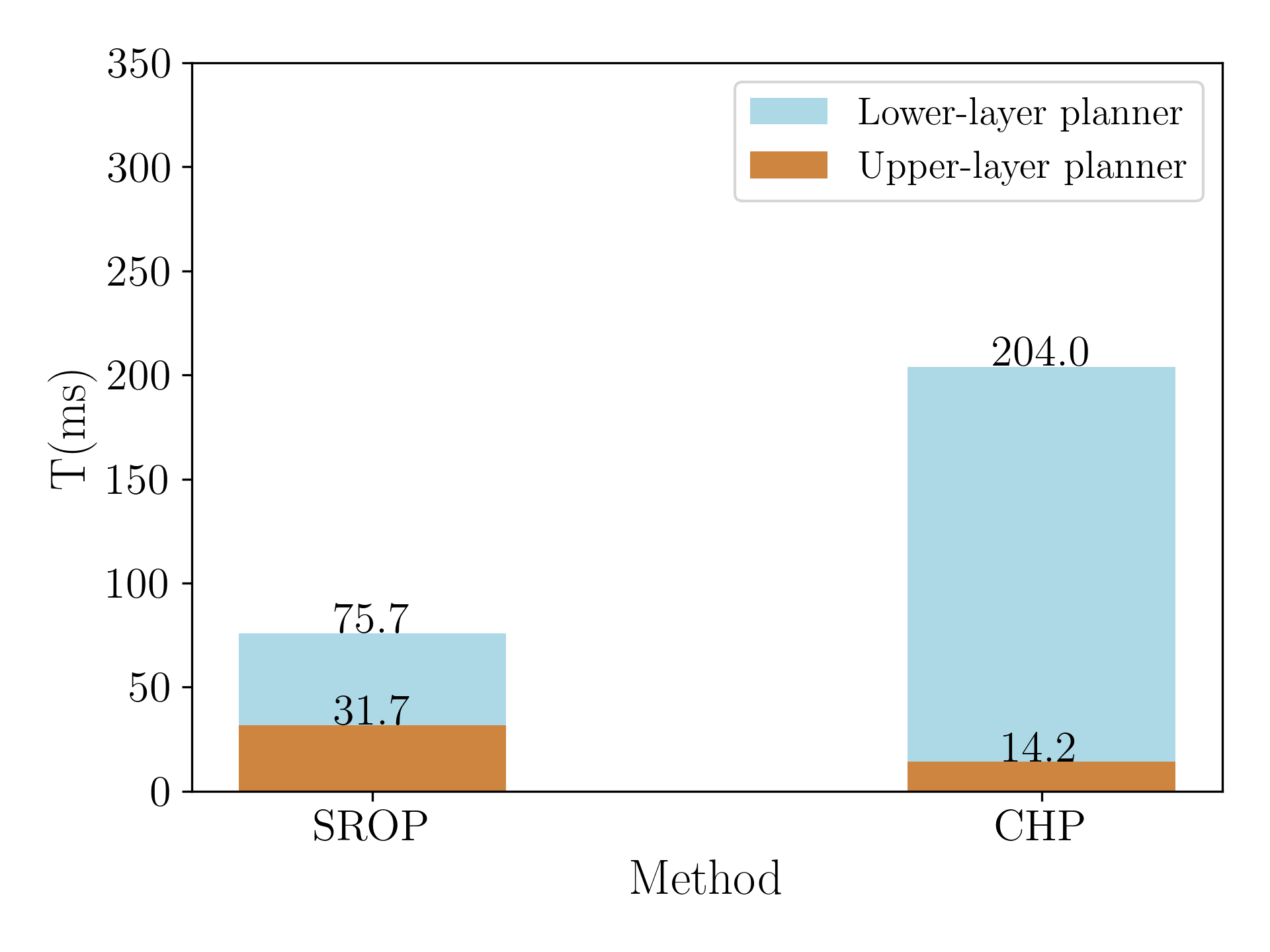
Figure 11: The time consumption comparison chart of SROP and CHP. The computation time of SROP decreased by 62.9% compared to CHP, indicating that SROP has significantly higher planning efficiency.

Based on the cost value $J_{\mathcal{E}}$ of the trajectory skeleton, we can identify the path with Topo ID #1 in scenarios S1, S2, and S3 for subsequent optimization. However, the final overtaking trajectories belong to different topological classes. This discrepancy arises because the distribution of obstacles means the solution space for the initial path may not always encompass the global optimum. Additionally, the initial path with the smallest $J_{\mathcal{E}}$ may be situated closer to obstacles.

During the optimization process conducted by the lower-layer planner, the value of $r_{a}$ is increased to improve control feasibility. However, this adjustment may also cause greater deformation of the optimized trajectory, leading to a higher risk of collisions. Conversely, initial paths with relatively larger values of $J_{\mathcal{E}}$ may allow for more deformation, which can ultimately result in better trajectory quality and enhanced control feasibility.

Table 8: Comparison of tracking performance and stability from different topological classes. The proposed STS method generates trajectories with superior tracking performance and stability across various topological classes.

Scenario	Topo ID	Tracking metrics
		$E_{p}$ ($m$)	$IP(E_{p})$	$E_{\theta}(rad)$	$IP(E_{\theta})$	$\omega(rad/s)$	$IP(\omega)$
S1	#11	0.106	-	0.068	-	0.221	-
	#2	0.101	4.7%	0.066	2.9%	0.215	2.7%
S2	#1	0.164	-	0.120	-	0.386	-
	#2	0.107	34.8%	0.079	34.2%	0.253	32.7%
S3	#1	0.134	-	0.107	-	0.344	-
	#3	0.108	19.4%	0.069	35.5%	0.253	26.5%
avg2.	-	-	19.6%	-	24.2%	-	20.6%

• The blue Topo ID represents the trajectory with the smallest $J_{\mathcal{E}}$
  within that trajectory topological class. The resluts of the Topo ID
  are the baseline for calculating the $IP(\cdot)$.

• The average value is calculated by averaging the $IP(\cdot)$ across all
  scenarios.

•   represents various metrics of the selected overtaking trajectory.

As shown in Table 8, the final overtaking trajectory exhibits notable improvements in both position tracking error $E_{p}$ and orientation angle error $E_{\theta}$ when compared to the trajectory with the smallest $J_{\mathcal{E}}$. Additionally, its average angular velocity $\omega_{m}$ is relatively lower. Across the three scenarios, the average reductions are 19.6% for $E_{p}$, 24.2% for $E_{\theta}$, and 20.6% for $\omega_{m}$.

The results indicate that the proposed method enhances trajectory quality compared to a single initial solution. This improvement arises from the ability of the method to generate initial paths from various topological classes for further optimization. Consequently, it avoids getting trapped in local optima, resulting in smoother trajectories and improved tracking performance.

6 Conclusion

This paper proposes a framework for planning overtaking trajectories to enhance time efficiency and ensure trajectory control feasibility. First, we present an efficient spatio-temporal topological search method that prevents getting stuck in local optima, thereby improves solution quality. Second, we incorporate the reachable set method into a parallel trajectory generation process to efficiently produce control-feasible trajectories. Finally, we introduce an overtaking hierarchical planning framework designed to improve both trajectory quality and time efficiency in dynamic scenarios.

Numerical simulation experiments show that our proposed method generates high-quality, efficient, and control-feasible trajectories. In comparison, state-of-the-art path planning algorithms typically produce a single collision-free initial path, which may cause trajectory refinement to become stuck in local optima. However, the proposed spatio-temporal topological search method considers multiple initial paths from various topological classes. Our method achieves a 19.6% reduction in trajectory tracking error and a 20.6% improvement in average smoothness, demonstrating significant enhancements in trajectory quality by avoiding local optimum entrapment. We introduce a parallel trajectory generation method based on reachable sets to improve planning efficiency. This approach effectively decouples the trajectory optimization problem from the nonlinear vehicle model, improving planning efficiency. We utilize reachable sets to evaluate the control feasibility of the generated trajectories. The tracking performance of these trajectories is assessed using a tracking controller based on a pure pursuit algorithm. When comparing the initial trajectory to the final trajectory produced by our method, the tracking error decreases by 40.3%. This outcome validates the effectiveness of reachable sets in assessing the feasibility of trajectory control. Additionally, when compared to the state-of-the-art hierarchical planning method, our framework demonstrates a 66.8% improvement in trajectory smoothness and a 62.9% reduction in computation time. This indicates that our proposed method offers better performance in terms of both trajectory quality and time efficiency.

In our future work, we aim to enhance topological path searching methods for quicker handling of complex scenarios. We plan to improve the extraction of reachable sets, using offline neural network training to link trajectories and reachable sets, enabling efficient online inference. This approach could significantly reduce planning time.

References

- Fan et al. [2018] H. Fan, F. Zhu, C. Liu, L. Zhang, L. Zhuang, D. Li, W. Zhu, J. Hu, H. Li, Q. Kong, Baidu apollo em motion planner, arXiv preprint arXiv:1807.08048 (2018).
- Lim et al. [2018] W. Lim, S. Lee, M. Sunwoo, K. Jo, Hierarchical trajectory planning of an autonomous car based on the integration of a sampling and an optimization method, IEEE Transactions on Intelligent Transportation Systems 19 (2018) 613–626.
- Xin et al. [2021] L. Xin, Y. Kong, S. E. Li, J. Chen, Y. Guan, M. Tomizuka, B. Cheng, Enable faster and smoother spatio-temporal trajectory planning for autonomous vehicles in constrained dynamic environment, Proceedings of the Institution of Mechanical Engineers, Part D: Journal of Automobile Engineering 235 (2021) 1101–1112.
- Liu et al. [2018] C. Liu, C.-Y. Lin, M. Tomizuka, The convex feasible set algorithm for real time optimization in motion planning, SIAM Journal on Control and optimization 56 (2018) 2712–2733.
- Li et al. [2020] B. Li, Q. Kong, Y. Zhang, Z. Shao, Y. Wang, X. Peng, D. Yan, On-road trajectory planning with spatio-temporal rrt* and always-feasible quadratic program, in: 2020 IEEE 16th International Conference on Automation Science and Engineering (CASE), IEEE, 2020, pp. 942–947.
- Li et al. [2024] Z. Li, L. Xie, C. Hu, H. Su, A rapid iterative trajectory planning method for automated parking through differential flatness, Robotics and Autonomous Systems 182 (2024) 104816.
- Hart et al. [1968] P. E. Hart, N. J. Nilsson, B. Raphael, A formal basis for the heuristic determination of minimum cost paths, IEEE transactions on Systems Science and Cybernetics 4 (1968) 100–107.
- Sniedovich [2006] M. Sniedovich, Dijkstra’s algorithm revisited: the dynamic programming connexion, Control and cybernetics 35 (2006) 599–620.
- Zhang et al. [2020] T. Zhang, M. Fu, W. Song, Y. Yang, M. Wang, Trajectory planning based on spatio-temporal map with collision avoidance guaranteed by safety strip, IEEE Transactions on Intelligent Transportation Systems 23 (2020) 1030–1043.
- Ajanovic et al. [2018] Z. Ajanovic, B. Lacevic, B. Shyrokau, M. Stolz, M. Horn, Search-based optimal motion planning for automated driving, in: 2018 IEEE/RSJ International Conference on Intelligent Robots and Systems (IROS), IEEE, 2018, pp. 4523–4530.
- Alarabi et al. [2022] S. Alarabi, C. Luo, M. Santora, A prm approach to path planning with obstacle avoidance of an autonomous robot, in: 2022 8th International Conference on Automation, Robotics and Applications (ICARA), IEEE, 2022, pp. 76–80.
- Sun et al. [2021] Y. Sun, C. Zhang, C. Liu, Collision-free and dynamically feasible trajectory planning for omnidirectional mobile robots using a novel b-spline based rapidly exploring random tree, International Journal of Advanced Robotic Systems 18 (2021) 17298814211016609.
- Wang et al. [2023] J. Wang, J. Li, J. Yang, X. Meng, T. Fu, Automatic parking trajectory planning based on random sampling and nonlinear optimization, Journal of the Franklin Institute 360 (2023) 9579–9601.
- Lin et al. [2021] Y. Lin, S. Maierhofer, M. Althoff, Sampling-based trajectory repairing for autonomous vehicles, in: 2021 IEEE International Intelligent Transportation Systems Conference (ITSC), IEEE, 2021, pp. 572–579.
- Li et al. [2022] X. Li, X. Gao, W. Zhang, L. Hao, Smooth and collision-free trajectory generation in cluttered environments using cubic b-spline form, Mechanism and Machine Theory 169 (2022) 104606.
- Rösmann et al. [2017] C. Rösmann, F. Hoffmann, T. Bertram, Integrated online trajectory planning and optimization in distinctive topologies, Robotics and Autonomous Systems 88 (2017) 142–153.
- Yi et al. [2018] B. Yi, P. Bender, F. Bonarens, C. Stiller, Model predictive trajectory planning for automated driving, IEEE Transactions on Intelligent Vehicles 4 (2018) 24–38.
- Zhou et al. [2020] B. Zhou, F. Gao, J. Pan, S. Shen, Robust real-time uav replanning using guided gradient-based optimization and topological paths, in: 2020 IEEE International Conference on Robotics and Automation (ICRA), IEEE, 2020, pp. 1208–1214.
- Ye et al. [2023] H. Ye, C. Xu, F. Gao, Std-trees: Spatio-temporal deformable trees for multirotors kinodynamic planning, in: 2023 IEEE International Conference on Robotics and Automation (ICRA), IEEE, 2023, pp. 1200–1206.
- de Groot et al. [2024] O. de Groot, L. Ferranti, D. Gavrila, J. Alonso-Mora, Topology-driven parallel trajectory optimization in dynamic environments, arXiv preprint arXiv:2401.06021 (2024).
- Ziegler et al. [2014] J. Ziegler, P. Bender, T. Dang, C. Stiller, Trajectory planning for bertha—a local, continuous method, in: 2014 IEEE intelligent vehicles symposium proceedings, IEEE, 2014, pp. 450–457.
- Gu et al. [2013] T. Gu, J. Snider, J. M. Dolan, J.-w. Lee, Focused trajectory planning for autonomous on-road driving, in: 2013 IEEE Intelligent Vehicles Symposium (IV), IEEE, 2013, pp. 547–552.
- Quirynen et al. [2024] R. Quirynen, S. Safaoui, S. Di Cairano, Real-time mixed-integer quadratic programming for vehicle decision-making and motion planning, IEEE Transactions on Control Systems Technology (2024).
- Han et al. [2023] Z. Han, Y. Wu, T. Li, L. Zhang, L. Pei, L. Xu, C. Li, C. Ma, C. Xu, S. Shen, et al., An efficient spatial-temporal trajectory planner for autonomous vehicles in unstructured environments, IEEE Transactions on Intelligent Transportation Systems (2023).
- Wu and Bayen [2022] F. Wu, A. M. Bayen, A hierarchical mpc approach to car-following via linearly constrained quadratic programming, IEEE Control Systems Letters 7 (2022) 532–537.
- Jain et al. [2019] V. Jain, U. Kolbe, G. Breuel, C. Stiller, Reacting to multi-obstacle emergency scenarios using linear time varying model predictive control, in: 2019 IEEE Intelligent Vehicles Symposium (IV), IEEE, 2019, pp. 1822–1829.
- Scheffe et al. [2022] P. Scheffe, T. M. Henneken, M. Kloock, B. Alrifaee, Sequential convex programming methods for real-time optimal trajectory planning in autonomous vehicle racing, IEEE Transactions on Intelligent Vehicles 8 (2022) 661–672.
- Li et al. [2022] Z. Li, J. Li, W. Wang, Path planning and obstacle avoidance control for autonomous multi-axis distributed vehicle based on dynamic constraints, IEEE Transactions on Vehicular Technology 72 (2022) 4342–4356.
- Micheli et al. [2023] F. Micheli, M. Bersani, S. Arrigoni, F. Braghin, F. Cheli, Nmpc trajectory planner for urban autonomous driving, Vehicle system dynamics 61 (2023) 1387–1409.
- Althoff and Dolan [2014] M. Althoff, J. M. Dolan, Online verification of automated road vehicles using reachability analysis, IEEE Transactions on Robotics 30 (2014) 903–918.
- Söntges and Althoff [2017] S. Söntges, M. Althoff, Computing the drivable area of autonomous road vehicles in dynamic road scenes, IEEE Transactions on Intelligent Transportation Systems 19 (2017) 1855–1866.
- Würsching and Althoff [2021] G. Würsching, M. Althoff, Sampling-based optimal trajectory generation for autonomous vehicles using reachable sets, in: 2021 IEEE International Intelligent Transportation Systems Conference (ITSC), IEEE, 2021, pp. 828–835.
- Manzinger et al. [2020] S. Manzinger, C. Pek, M. Althoff, Using reachable sets for trajectory planning of automated vehicles, IEEE Transactions on Intelligent Vehicles 6 (2020) 232–248.
- Liu et al. [2024] Y. Liu, X. Pei, H. Zhou, X. Guo, Spatiotemporal trajectory planning for autonomous vehicle based on reachable set and iterative lqr, IEEE Transactions on Vehicular Technology (2024).
- Jewell [2021] N. C. Jewell, Embedded reachability for autonomous racecar (2021).
- Althoff et al. [2011] M. Althoff, C. Le Guernic, B. H. Krogh, Reachable set computation for uncertain time-varying linear systems, in: Proceedings of the 14th international conference on Hybrid systems: computation and control, 2011, pp. 93–102.
- Werling et al. [2012] M. Werling, S. Kammel, J. Ziegler, L. Gröll, Optimal trajectories for time-critical street scenarios using discretized terminal manifolds, The International Journal of Robotics Research 31 (2012) 346–359.
- Richter et al. [2016] C. Richter, A. Bry, N. Roy, Polynomial trajectory planning for aggressive quadrotor flight in dense indoor environments, in: Robotics Research: The 16th International Symposium ISRR, Springer, 2016, pp. 649–666.
- Murray et al. [1995] R. M. Murray, M. Rathinam, W. Sluis, Differential flatness of mechanical control systems: A catalog of prototype systems, in: ASME international mechanical engineering congress and exposition, Citeseer, 1995, pp. 349–357.
- Fu et al. [2022] J. Fu, Z. Jian, P. Chen, S. Chen, J. Xin, N. Zheng, Integrated global path planning for autonomous mobile robots in complicated environments, in: 2022 IEEE 25th International Conference on Intelligent Transportation Systems (ITSC), IEEE, 2022, pp. 1381–1387.
- Zuo et al. [2020] Z. Zuo, X. Yang, Z. Li, Y. Wang, Q. Han, L. Wang, X. Luo, Mpc-based cooperative control strategy of path planning and trajectory tracking for intelligent vehicles, IEEE Transactions on Intelligent Vehicles 6 (2020) 513–522.
- Ahn et al. [2021] J. Ahn, S. Shin, M. Kim, J. Park, Accurate path tracking by adjusting look-ahead point in pure pursuit method, International journal of automotive technology 22 (2021) 119–129.