High-genus KdV soliton gases and their long-time asymptotics

Abstract

This paper employs the Riemann-Hilbert problem to provide a comprehensive analysis of the asymptotic behavior of the high-genus Korteweg-de Vries soliton gases. It is demonstrated that the two-genus soliton gas is related to the two-phase Riemann-Theta function as $x\to+\infty$, and approaches to zero as $x\to-\infty$. Additionally, the long-time asymptotic behavior of this two-genus soliton gas can be categorized into five distinct regions in the $x$-$t$ plane, which from left to right are rapidly decay, modulated one-phase wave, unmodulated one-phase wave, modulated two-phase wave, and unmodulated two-phase wave. Moreover, an innovative method is introduced to solve the model problem associated with the high-genus Riemann surface, leading to the determination of the leading terms, which is also related with the multi-phase Riemann-Theta function. A general discussion on the case of arbitrary $N$-genus soliton gas is also presented.

Key words: KdV equation, Riemann-Hilbert problem, soliton gas

AMS subjectclassi cations: 35Q15,35Q51,35Q53

1 Introduction

It is well known that the Korteweg-de Vries (KdV) equation

$$u_{t}-6uu_{x}+u_{xxx}=0$$ (1.0.1)

can be presented as the compatibility condition of the Lax pair [24]

$$(-\partial_{xx}+u)\varphi(x,t)=E\varphi(x,t),$$ (1.0.2)

$$\varphi_{t}(x,t)=(4\partial_{x}-6u\partial_{x}-3u_{x})\varphi(x,t),$$

where $E$ is the spectral parameter. Based on the Lax pair formulation (1.0.2), extensive researches have been conducted on the KdV equation (1.0.1) by using the inverse scattering transform [1, 7, 27] and Riemann-Hilbert formulation [13, 16]. One of the most notable results is the existence of a special class of localized wave solutions known as solitons. The simplest example of a single soliton solution is given by

$$u(x,t)=-2\eta^{2}\operatorname{sech}^{2}(\eta(x-4\eta^{2}t-x_{0})),$$ (1.0.3)

where the spectral parameter is $E=\eta^{2}$, and $x_{0}$ is the phase parameter that determines the initial position of the soliton. In this context, the position is defined by the location of the maximum of the soliton profile. On the other hand, the KdV equation admits the periodic traveling wave solution of the form [22, 23]

$$u(x,t)=k_{2}+\left(k_{1}-k_{2}\right)\mathrm{cn}^{2}\left(\frac{\sqrt{k_{1}-k_{3}}}{\sqrt{2}}\left(x-2(k_{1}+k_{2}+k_{3})t+\frac{\phi_{0}}{k}\right)-K(m);m\right),$$ (1.0.4)

where $k_{1}>k_{2}>k_{3}$, ${\mathrm{cn}}(s;m)$ is the Jacobi elliptic function and $K(m)$ is a complete elliptic integral of the first kind, i.e., $K(m):=\int_{0}^{\frac{\pi}{2}}\frac{d\vartheta}{\sqrt{1-m^{2}\sin^{2}\vartheta}}$ with $m=\frac{k_{1}-k_{2}}{k_{1}-k_{3}}$ and $k=\pi\frac{\sqrt{k_{1}-k_{3}}}{\sqrt{2}K(m)}$. Especially, as $k_{2}\to k_{3}$, the periodic solution (1.0.4) degenerates into the soliton solution by the identity $\mathrm{cn}(\bullet;1)=\mathrm{sech}(\bullet)$.

In 1971, Zakharov [33] first introduced the concept of “soliton gas” and derived an integro-differential kinetic equation for the soliton gas by evaluating the efficient modification of the soliton velocity within a rarefied gas. Specifically, he treated solitons as “particles”, and a soliton gas can be understood as a collection of randomly distributed solitons, resembling the behavior of a gas [31]. Forty-five years later, in 2016, Zakharov and his collaborators [15] revisited the soliton gas for the KdV equation by using the dressing method and proposed an alternate construction of the Bargmann potentials. In particular, they formulated a Riemann-Hilbert problem (RH problem) associated with the soliton gas, given as follows:

$$\Xi^{+}(i\kappa)=M(x,\kappa)\Xi^{-}(i\kappa),\quad\Xi^{+}(-i\kappa)=M^{T}(x,\kappa)\Xi^{-}(-i\kappa),$$ (1.0.5)

$$M(x,\kappa)=\frac{1}{1+R_{1}R_{2}}\left[\begin{array}[]{ll}1-R_{1}R_{2}&2iR_{1}e^{-2\kappa x}\\ 2iR_{2}e^{2\kappa x}&1-R_{1}R_{2}\end{array}\right],$$

where $\Xi:\mathbb{C}\to\mathbb{C}^{2}$ is a vector-valued function, and $\kappa\in[k_{1},k_{2}]$ with $0<k_{1}<k_{2}$. Although research on soliton gas began many years ago, the understanding of the properties of an interacting ensemble of large solitons and their dynamic behavior, even in the absence of randomness, remains incomplete from a mathematically precise perspective. In 2003, El [17, 11] proposed a unified extension of Zakharov’s kinetic equation for the KdV dense soliton gas by considering the thermodynamic limit of KdV–Whitham equations. Subsequently, the kinetic equation for soliton gas was examined for its diverse and complex mathematical characteristics [2, 18, 19]. In addition, Bertola et al. derived the kinetic equation for the KdV equation by using the method of genus degeneration in [3]. Recently, Girotti and her collaborators [20] investigated the one-genus KdV soliton gas and established an asymptotic description of soliton gas dynamics for large time by using the Deift-Zhou nonlinear steepest descent method [12]. They [21] also investigated the behaviors of a trial soliton travelling through a mKdV soliton gas and built the kinetic theory for soliton gas. For a concise relationship between the mKdV equation and KdV equation, please refer to [10]. In fact, the results presented in [20, 21] represent a particular case of (1.0.5) for $R_{2}=0$, involving only two disjoint stability zones. Furthermore, the study of soliton gas for the NLS equation was examined in [5, 6, 9, 29], and the relationship between periodic potentials was explored in [26].

This paper investigates the high-genus soliton gas for the KdV equation (1.0.1), focusing specifically on the two-genus soliton gas potential and its long-time asymptotics. More precisely, we consider the special case of (1.0.5) with $R_{1}=0$ and $R_{2}=r_{2}(\lambda)$, which involves four disjoint stability zones. Suppose $0<\eta_{1}<\eta_{2}<\eta_{3}<\eta_{4}$ and let $\Sigma_{1}:=(\eta_{1},\eta_{2})$, $\Sigma_{2}:=(-\eta_{2},-\eta_{1})$, $\Sigma_{3}:=(\eta_{3},\eta_{4})$, and $\Sigma_{4}:=(-\eta_{4},-\eta_{3})$. Additionally, denote $\Sigma_{i,\cdots,k}=\Sigma_{i}\cup\cdots\cup\Sigma_{k}$. We then construct the following RH problem for the vector-valued function $X(\lambda)$ as

$$X_{+}(\lambda)=X_{-}(\lambda)\begin{cases}\begin{aligned} &\begin{pmatrix}1&-2ir_{2}(\lambda)e^{-2i\lambda x}\\ 0&1\end{pmatrix},&&\lambda\in i\Sigma_{1,3},\\ &\begin{pmatrix}1&0\\ 2ir_{2}(\lambda)e^{2i\lambda x}&1\end{pmatrix},&&\lambda\in i\Sigma_{2,4},\end{aligned}\end{cases}$$ (1.0.6)

$$X(\lambda)\to\begin{pmatrix}1&1\end{pmatrix},\quad\lambda\to\infty,$$ (1.0.7)

$$X(-\lambda)=X(\lambda)\begin{pmatrix}0&1\\ 1&0\end{pmatrix}.$$ (1.0.8)

Then the two-genus soliton gas potential of the KdV equation (1.0.1) is given by the reconstruction formula

$$u(x)=2\frac{\mathrm{d}}{\mathrm{d}x}\left(\lim_{\lambda\to\infty}\frac{\lambda}{i}\left(X_{1}(\lambda)-1\right)\right),$$ (1.0.9)

where $X_{1}(\lambda)$ is the first component of $X(\lambda)$.

In what follows, we propose the main results of this work.

1.1 Statement of the main results

Firstly, a two-genus KdV soliton gas potential (1.0.9) is constructed by formulating the Riemann-Hilbert problem (1.0.6)-(1.0.8) from the pure $N$-soliton Riemann-Hilbert problem in Section 2 for $N\to+\infty$, where the initial positions of the $N$ solitons are located on the positive real axis. Then, in Section 3, we establish the large $x$ behaviors of this soliton gas potential in Theorem 1.1.1.

Theorem 1.1.

The potential function $u(x)$, which satisfies the reconstruction formula (1.0.9) and the Riemann-Hilbert problem (1.0.6)-(1.0.8), exhibits the following asymptotic behaviors:

$$u(x)=\begin{cases}\begin{aligned} &-\left(2\alpha+{\sum_{j=1}^{4}\eta_{j}^{2}}+2\partial_{x}^{2}\log\left(\Theta\left(\frac{\Omega}{2\pi i};\hat{\tau}\right)\right)\right)+\mathcal{O}\left(\frac{1}{x}\right),&&x\to+\infty,\\ &\mathcal{O}(e^{-c|x|}),&&x\to-\infty.\end{aligned}\end{cases}$$ (1.1.1)

Here, $\Theta(\bullet;\hat{\tau})$ denotes the two-phase Riemann-Theta function defined by (3.1.3), $\Omega$ is a two-dimensional column vector given by (3.1.5) and the imaginary part of the period matrix $\hat{\tau}$, as defined in (3.2.4), is positive definite. Furthermore, the parameter $\alpha$ is defined in Remark 3.1, and $c$ is a fixed positive constant.

Indeed, the initial situation can be viewed as two interlocking one-genus soliton gases. As time develops, the two “gases” will collide with each other, with the faster gas transcending the slower one. Consequently, the slower gas generates both modulated and unmodulated one-phase waves, similar to the case described in [20]. The collision region corresponds to the modulated two-phase wave, while the unmodulated wave represents the region without collisions. Figure 1 presents a direct numerical simulation of the KdV equation (1.0.1) with initial potential (1.0.9) behaving the asymptotics in equation (1.1.1) with parameters $\eta_{1}=0.8$, $\eta_{2}=1.2$, $\eta_{3}=1.6$, $\eta_{4}=2$, and $r_{2}(\lambda)=1$. The Figure 1 clearly shows that the plane is divided into five distinct regions, which from left to right are rapid decay region, modulated one-phase wave region, unmodulated one-phase wave region, modulated two-phase wave region and unmodulated two-phase wave region.

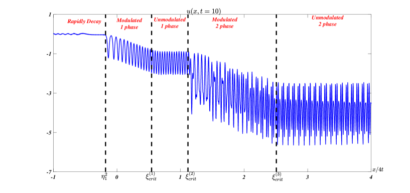
Figure 1: The evolution of the two-genus soliton gas potential of the KdV equation at $t=10$ for parameters $\eta_{1}=0.8$, $\eta_{2}=1.2$, $\eta_{3}=1.6$, $\eta_{4}=2$, and $r_{2}(\lambda)=1$. The horizontal axis represents $\frac{x}{4t}$, and the critical points $\eta_{1}^{2}$ and $\xi_{\text{crit}}^{(j)}$ for $j=1,2,3$ partition the plane into five distinct regions. These critical values, $\xi_{\text{crit}}^{(j)}$, can be calculated by using equations (4.3.9) and (4.1.10) approximately. For the given parameters, the approximate values are $\xi_{\text{crit}}^{(1)}\approx 2.090525$, $\xi_{\text{crit}}^{(2)}\approx 3.2338$, and $\xi_{\text{crit}}^{(3)}\approx 6.015613$.

More precisely, the long-time asymptotics of $u(x,t)$ for the two-genus KdV soliton gas potential depends on the parameter $\xi:=\frac{x}{4t}$. There are four critical values, i.e., $\eta_{1}^{2}$ and $\xi_{\text{crit}}^{(j)}$ for $j=1,2,3$, defined in equations (4.1.10) and (4.3.9), which serve as the boundaries between different regions, as illustrated in Figure 2 and Theorem 1.2 below. The proof of Theorem 1.2 will be provided in detail in Section 4.

Figure 2: Five asymptotic regions of the two-genus KdV soliton gas potential in the $x$-$t$ half plane.

Theorem 1.2.

As $t\to+\infty$, the global long-time asymptotic behaviors of $u(x,t)$ for the KdV equation with initial potential (1.0.9) behaving the asymptotics in equation (1.1.1) can be described as follows:

1. For fixed $\xi<\eta_{1}^{2}$, there exists a positive constant $c$ such that

   $$u(x,t)=\mathcal{O}\left(e^{-ct}\right).$$

2. For $\eta_{1}^{2}<\xi<\xi_{\text{crit}}^{(1)}$, the long-time asymptotics of $u(x,t)$ can be described by a Jacobi elliptic function “$\mathrm{dn}$” with modulated parameter $\alpha_{1}$ and modulated modulus $m_{\alpha_{1}}=\frac{\eta_{1}}{\alpha_{1}}$ as

   $$u(x,t)=\alpha_{1}^{2}-\eta_{1}^{2}-2\alpha_{1}^{2}\mathrm{dn}^{2}\left(\alpha_{1}\left(x-2(\alpha_{1}^{2}+\eta_{1}^{2})t+\phi_{\alpha_{1}}\right)+K(m_{\alpha_{1}});m_{\alpha_{1}}\right)+\mathcal{O}\left(\frac{1}{t}\right),$$

   where the parameter $\alpha_{1}$ is determined by equation (4.1.8) and

   $$\phi_{\alpha_{1}}=\int_{\alpha_{1}}^{\eta_{1}}\frac{\log r(\zeta)}{R_{\alpha_{1},+}(\zeta)}\frac{d\zeta}{\pi i},$$

   and $K(m_{\alpha_{1}})$ is the complete elliptic integral of the first kind, defined as $K(m_{\alpha_{1}})=\int_{0}^{\frac{\pi}{2}}\frac{d\vartheta}{\sqrt{1-m_{\alpha_{1}}^{2}\sin^{2}\vartheta}}$.

3. For $\xi_{\text{crit}}^{(1)}<\xi<\xi_{\text{crit}}^{(2)}$, the long-time asymptotics of $u(x,t)$ can be described by a Jacobi elliptic function “$\mathrm{dn}$” with constant coefficients below

   $$u(x,t)=\eta_{2}^{2}-\eta_{1}^{2}-2\eta_{2}^{2}\mathrm{dn}^{2}\left(\eta_{2}(x-2(\eta_{2}^{2}+\eta_{1}^{2})t+\phi_{\eta_{2}})+K(m_{\eta_{2}});m_{\eta_{2}}\right)+\mathcal{O}\left(\frac{1}{t}\right),$$

   where $m_{\eta_{2}}=\frac{\eta_{1}}{\eta_{2}}$, and

   $$\phi_{\eta_{2}}=\int_{\eta_{2}}^{\eta_{1}}\frac{\log r(\zeta)}{R_{\eta_{2},+}(\zeta)}\frac{d\zeta}{\pi i}.$$

4. For $\xi_{\text{crit}}^{(2)}<\xi<\xi_{\text{crit}}^{(3)}$, the long-time asymptotics of $u(x,t)$ can be described by the modulated two-phase wave

   $$u(x,t)=-\left(2b_{\alpha_{2},1}+\sum_{j=1}^{3}\eta_{j}^{2}+\alpha_{2}^{2}+2\partial_{x}^{2}\log\left(\Theta\left(\frac{\Omega_{\alpha_{2}}}{2\pi i};\hat{\tau}_{\alpha_{2}}\right)\right)\right)+\mathcal{O}\left(\frac{1}{t}\right),$$ (1.1.2)

   where the constant $b_{\alpha_{2},1}$ is determined by equation (4.3.6), parameter $\alpha_{2}$ is determined by equation (4.3.7) and the period matrix $\hat{\tau}_{\alpha_{2}}$ is given in equation (4.3.16).

5. For fixed $\xi_{\text{crit}}^{(3)}<\xi$, the long-time asymptotics of $u(x,t)$ can be described by the unmodulated two-phase wave

   $$u(x,t)=-\left(2b_{\eta_{4},1}+{\sum_{j=1}^{4}\eta_{j}^{2}}+2\partial_{x}^{2}\log\left(\Theta\left(\frac{\Omega_{\eta_{4}}}{2\pi i};\hat{\tau}_{\eta_{4}}\right)\right)\right)+\mathcal{O}\left(\frac{1}{t}\right),$$

   where $\hat{\tau}_{\eta_{4}}=\hat{\tau}$ in (3.2.4) and $b_{\eta_{4}},\Omega_{\eta_{4}}=\begin{pmatrix}{t\Omega_{\eta_{4},1}+{\Delta_{\eta_{4},1}}}&{t\Omega_{\eta_{4},0}+{\Delta_{\eta_{4},0}}}\end{pmatrix}^{T}$ are defined by (4.3.6) and (4.3.17), respectively.

In fact, the method for genus-two KdV soliton gas can be generalized to investigate the soliton gases of arbitrary genus. In Section 5, the construction of KdV soliton gases of general genus $\mathcal{N}$ is discussed, along with a preliminary analysis of their evolutionary properties.

1.2 Some remarks on Theorem 1.1 and Theorem 1.2

It will be seen that the studies of asymptotic behaviors of the two-genus KdV soliton gas potential (1.0.9) are not the trivial generalization of that in the one-genus KdV soliton gas potential in [20]. The leading-order term in asymptotic expression (1.1.2) also arises from the context of the small-dispersion limit of the KdV equation, as discussed in [8, 14]. Although the initial RH problem (1.0.6)-(1.0.8) involves four jump bands, corresponding to a three-genus scenario, after applying the holomorphic map $z=-\lambda^{2}$ and by using the Riemann-Hurwitz formula, the corresponding Riemann surface is indeed of genus two. Moreover, the model problem associated with this new Riemann surface resembles the one in [14], and this approach can be extended to higher-genus cases.

2 Construction of two-genus KdV soliton gas potential

It is known that a pure $N$-soliton solution of the KdV equation (1.0.1) associates with a vector-valued RH problem. To be specific, let $M(\lambda)$ be a $1\times 2$ vector satisfying:

(i) $M(\lambda)$ is meromorphic in the whole complex plane, with simple poles at $\left\{\lambda_{j}\right\}_{j=1}^{N}$ in $i\mathbb{R}_{+}$ and the corresponding conjugate points $\left\{\bar{\lambda}_{j}\right\}_{j=1}^{N}$ in $i\mathbb{R}_{-}$;

(ii) The following residue conditions for $M(\lambda)$ hold

$$\underset{\lambda=\lambda_{j}}{\operatorname{res}}M(\lambda)=\lim_{\lambda\rightarrow\lambda_{j}}M(\lambda)\begin{pmatrix}0&\frac{c_{j}e^{-2i\lambda_{j}x}}{N}\\ 0&0\end{pmatrix},\quad\underset{\lambda=\bar{\lambda}_{j}}{\operatorname{res}}M(\lambda)=\lim_{\lambda\rightarrow\bar{\lambda}_{j}}M(\lambda)\begin{pmatrix}0&0\\ \frac{-c_{j}e^{2i\bar{\lambda}_{j}x}}{N}&0\end{pmatrix},$$

where $c_{j}\in i\mathbb{R}_{+},$ $j=1,\cdots,N$;

(iii) $M(\lambda)$ satisfies the asymptotics $M(\lambda)=\left(\begin{array}[]{ll}1&1\end{array}\right)+\mathcal{O}\left(\frac{1}{\lambda}\right)$ for $\lambda\rightarrow\infty$;

(iv) $M$ admits the symmetry

$$M(-\lambda)=M(\lambda)\left(\begin{array}[]{ll}0&1\\ 1&0\end{array}\right).$$

The stationary $N$-soliton solution of the KdV equation (1.0.1) is constructed by

$$u(x)=2\frac{\mathrm{d}}{\mathrm{d}x}\left(\lim_{\lambda\rightarrow\infty}\frac{\lambda}{i}\left(M_{1}(\lambda)-1\right)\right),$$

where $M_{1}(\lambda)$ is the first element of row vector $M(\lambda)$. Specially, for $N=1$ and taking $\lambda_{1}=i\eta,c_{1}=ic,c>0$, the stationary one-soliton solution of the KdV equation (1.0.1) is derived as

$$u(x)=-2\eta^{2}\operatorname{sech}^{2}\left(\eta\left(x-x_{0}\right)\right),$$

which is a time-independent version of the single soliton solution (1.0.3) with initial position

$$x_{0}=\frac{1}{2\eta}\log\frac{2\eta}{c}\in\mathbb{R}.$$

Reminding the notations $\Sigma_{j}~{}(j=1,2,3,4)$ above, for the sake of simplicity, when considering $N\to+\infty$ restricted on the four bands $(i\eta_{1},i\eta_{2}),(i\eta_{3},i\eta_{4}),(-i\eta_{2},-i\eta_{1})$ and $(-i\eta_{4},-i\eta_{3})$ respectively, we take the following assumptions.

Assumption 1.

Assume the next three items hold:

1. Divide $\{\lambda_{j}\}_{j=1}^{N}$ into two parts, that are $\{\lambda_{l}\}_{l=1}^{N_{1}}$ and $\{\lambda_{k}\}_{k=1}^{N_{2}}$, with $N_{1}+N_{2}=N$. Suppose the $N_{1}$ poles are uniformly distributed on $(i\eta_{1},i\eta_{2})$, while the $N_{2}$ poles are uniformly distributed on $(i\eta_{3},i\eta_{4})$. More explicitly, let $|\lambda_{l+1}-\lambda_{l}|=\frac{\eta_{2}-\eta_{1}}{N_{1}}$ and $|\lambda_{k+1}-\lambda_{k}|=\frac{\eta_{4}-\eta_{3}}{N_{2}}$.

2. Similarly, the coefficients $c_{j}$ are also divided into two groups, i.e., $\{c_{l}\}_{l=1}^{N_{1}},\{c_{k}\}_{k=1}^{N_{2}}$, and are purely imaginary. Moreover, assume that

   $$c_{l}=\frac{i(\eta_{2}-\eta_{1})r_{2}(\lambda_{l})}{\pi},~{}l=1,2,\cdots,N_{1},$$

   $$c_{k}=\frac{i(\eta_{4}-\eta_{3})r_{2}(\lambda_{k})}{\pi},~{}k=1,2,\cdots,N_{2},$$

   where $r_{2}(\lambda)$ is an analytic function for $\lambda$ near $i\Sigma_{1,2,3,4}$, with symmetry $r_{2}(\bar{\lambda})=r_{2}(\lambda)$. Moreover, $r_{2}(\lambda)$ is assumed to be a real-valued positive nonvanishing function for $\lambda$ in the closure of $\Sigma_{1,2,3,4}$.

3. Indeed, we only consider the case that $N_{1}\to+\infty$ and $N_{2}\to+\infty$, simultaneously.

Note that the corresponding conjugate points $\left\{\bar{\lambda}_{j}\right\}_{j=1}^{N}$ are considered in the same way on $(-i\eta_{2},-i\eta_{1})$ and $(-i\eta_{4},-i\eta_{3})$. Now, remove the poles in $M(\lambda)$ by taking the transformations

$$Z(\lambda)=\begin{cases}\begin{aligned} &M(\lambda)\begin{pmatrix}1&-\frac{1}{N}\sum_{j=1}^{N}\frac{c_{j}e^{-2i\lambda x}}{\lambda-\lambda_{j}}\\ 0&1\end{pmatrix},&&\lambda\ \text{within}\ \gamma_{+},\\ &M(\lambda)\begin{pmatrix}1&0\\ \frac{1}{N}\sum_{j=1}^{N}\frac{c_{j}e^{2i\lambda x}}{\lambda+\lambda_{j}}&1\end{pmatrix},&&\lambda\ \text{within}\ \gamma_{-},\end{aligned}\end{cases}$$

where $\gamma_{+}$ is a counter clockwise contour, which surrounds the interval $(i\eta_{1},i\eta_{2})$ and $(i\eta_{3},i\eta_{4})$ in the upper half plane, and $\gamma_{-}$is a clockwise contour, which surrounds the interval $(-i\eta_{2},-i\eta_{1})$ and $(-i\eta_{4},-i\eta_{3})$ in the lower half plane. Consequently, the jump conditions for function $Z(\lambda)$ are converted into

$$Z_{+}(\lambda)=Z_{-}(\lambda)\begin{cases}\begin{aligned} &\begin{pmatrix}1&-\frac{1}{N}\sum_{j=1}^{N}\frac{c_{j}e^{-2i\lambda x}}{\lambda-\lambda_{j}}\\ 0&1\end{pmatrix},&&\lambda\in\gamma_{+},\\ &\begin{pmatrix}1&0\\ -\frac{1}{N}\sum_{j=1}^{N}\frac{c_{j}e^{2i\lambda x}}{\lambda+\lambda_{j}}&1\end{pmatrix},&&\lambda\in\gamma_{-}.\end{aligned}\end{cases}$$

As $N_{1},N_{2}\to+\infty$, one has $N=N_{1}+N_{2}\to+\infty$. For any open set $U_{1}$ containing $i\Sigma_{1}\cup i\Sigma_{3}$, the series converges uniformly for all $\lambda\in\mathbb{C}\setminus U_{1}$, that is

$$\mathop{{\rm lim}}\limits_{N\to+\infty}\frac{1}{N}\sum_{j=1}^{N}\frac{c_{j}}{\lambda-\lambda_{j}} =\mathop{{\rm lim}}\limits_{N_{1}\to+\infty}\frac{1}{N_{1}}\sum_{l=1}^{N_{1}}\frac{1}{\lambda-\lambda_{l}}\frac{(\eta_{2}-\eta_{1})ir_{2}(\lambda_{l})}{\pi}+\mathop{{\rm lim}}\limits_{N_{2}\to+\infty}\frac{1}{N_{2}}\sum_{k=1}^{N_{2}}\frac{1}{\lambda-\lambda_{k}}\frac{(\eta_{4}-\eta_{3})ir_{2}(\lambda_{k})}{\pi}$$

$$=\int_{i\eta_{1}}^{i\eta_{2}}\frac{2ir_{2}(\zeta)}{\lambda-\zeta}\frac{d\zeta}{2\pi i}+\int_{i\eta_{3}}^{i\eta_{4}}\frac{2ir_{2}(\zeta)}{\lambda-\zeta}\frac{d\zeta}{2\pi i}.$$

Similarly, for any open set $U_{2}$ containing $i\Sigma_{2}\cup i\Sigma_{4}$, the series converges uniformly for all $\lambda\in\mathbb{C}\setminus U_{2}$, that is

$$\mathop{{\rm lim}}\limits_{N\to+\infty}\frac{1}{N}\sum_{j=1}^{N}\frac{c_{j}}{\lambda+\lambda_{j}}=\int_{-i\eta_{2}}^{-i\eta_{1}}\frac{2ir_{2}(\zeta)}{\zeta-\lambda}\frac{d\zeta}{2\pi i}+\int_{-i\eta_{4}}^{-i\eta_{3}}\frac{2ir_{2}(\zeta)}{\zeta-\lambda}\frac{d\zeta}{2\pi i}.$$

As result, a limiting RH problem for $Z(\lambda)$ is obtained below

$$Z_{+}(\lambda)=Z_{-}(\lambda)\begin{cases}\begin{aligned} &\begin{pmatrix}1&e^{-2i\lambda x}(\int_{i\eta_{1}}^{i\eta_{2}}\frac{2ir_{2}(\zeta)}{\zeta-\lambda}\frac{d\zeta}{2\pi i}+\int_{i\eta_{3}}^{i\eta_{4}}\frac{2ir_{2}(\zeta)}{\zeta-\lambda}\frac{d\zeta}{2\pi i})\\ 0&1\end{pmatrix},&&\lambda\in\gamma_{+},\\ &\begin{pmatrix}1&0\\ e^{2i\lambda x}(\int_{-i\eta_{2}}^{-i\eta_{1}}\frac{2ir_{2}(\zeta)}{\zeta-\lambda}\frac{d\zeta}{2\pi i}+\int_{-i\eta_{4}}^{-i\eta_{3}}\frac{2ir_{2}(\zeta)}{\zeta-\lambda}\frac{d\zeta}{2\pi i})&1\end{pmatrix},&&\lambda\in\gamma_{-},\\ \end{aligned}\end{cases}$$

$$Z(\lambda)=\left(\begin{array}[]{ll}1&1\end{array}\right)+\mathcal{O}\left(\frac{1}{\lambda}\right),\quad\text{for}\quad\lambda\to\infty.$$

Now, comprassing the jump conditions of $Z(\lambda)$ on the contour $\gamma_{\pm}$ into jumps on $\Sigma_{1,2,3,4}$ by defining

$$X(\lambda)=\begin{cases}\begin{aligned} &Z(\lambda)\begin{pmatrix}1&-e^{-2i\lambda x}(\int_{i\eta_{1}}^{i\eta_{2}}\frac{2ir_{2}(\zeta)}{\zeta-\lambda}\frac{d\zeta}{2\pi i}+\int_{i\eta_{3}}^{i\eta_{4}}\frac{2ir_{2}(\zeta)}{\zeta-\lambda}\frac{d\zeta}{2\pi i})\\ 0&1\end{pmatrix},&&\lambda\ \text{within}\ \gamma_{+},\\ &Z(\lambda)\begin{pmatrix}1&0\\ e^{2i\lambda x}(\int_{-i\eta_{2}}^{-i\eta_{1}}\frac{2ir_{2}(\zeta)}{\zeta-\lambda}\frac{d\zeta}{2\pi i}+\int_{-i\eta_{4}}^{-i\eta_{3}}\frac{2ir_{2}(\zeta)}{\zeta-\lambda}\frac{d\zeta}{2\pi i})&1\end{pmatrix},&&\lambda\ \text{within}\ \gamma_{-},\\ &Z(\lambda),&&\lambda\ \text{outside}\ \gamma_{\pm}.\end{aligned}\end{cases}$$

By using the Plemelj formula, the RH problem for function $X(\lambda)$ in (1.0.6)-(1.0.8) is derived immediately. Finally, transform the RH problem on contours $i\Sigma_{1,2,3,4}$ into that on contours $\Sigma_{1,2,3,4}$ by defining $Y(\lambda)=X(i\lambda),\ r(\lambda)=2r_{2}(i\lambda)$, then we arrive at the RH problem for the soliton gas potential of the KdV equation as follows.

The function $Y(\lambda)$ is analytic for $\lambda\in\mathbb{C}\setminus\Sigma_{1,2,3,4}$ with $\Sigma_{1,2,3,4}:=\Sigma_{1}\cup\Sigma_{2}\cup\Sigma_{3}\cup\Sigma_{4}$, and has the properties:

$$Y_{+}(\lambda)=Y_{-}(\lambda)\begin{cases}{\left(\begin{array}[]{cc}1&-ir(\lambda)e^{2\lambda x}\\ 0&1\end{array}\right)},&\lambda\in\Sigma_{1,3},\\ {\left(\begin{array}[]{cc}1&0\\ ir(\lambda)e^{-2\lambda x}&1\end{array}\right)},&\lambda\in\Sigma_{2,4},\end{cases}$$

$$Y(\lambda)=(1\quad 1)+\mathcal{O}\left(\frac{1}{\lambda}\right),$$

$$Y(-\lambda)=Y(\lambda)\left(\begin{matrix}0&1\\ 1&0\end{matrix}\right).$$

So the KdV soliton gas potential can be reformulated by

$$u(x)=2\frac{\mathrm{d}}{\mathrm{d}x}\left(\lim_{\lambda\rightarrow\infty}{\lambda}\left(Y_{1}(\lambda;x)-1\right)\right),$$

where $Y_{1}(\lambda)$ is the first component of vector-valued function $Y(\lambda)$.

Lemma 2.1.

The solution to the RH problem concerning row vector $Y(\lambda)$ stated above exists and is unique.

Proof.

Rewrite row vector $Y(\lambda)$ as $(y^{1}(\lambda),y^{2}(\lambda))$. Combining the jump conditions on $\Sigma_{2,4}$, it is deduced that

$$y^{1}_{+}(\lambda)=y^{1}_{-}(\lambda)-ir(\lambda)y^{2}_{+}(\lambda),\quad y^{2}_{+}(\lambda)=y^{2}_{-}(\lambda).$$

It is evident that $y^{2}(\lambda)$ is holomorphic across $\Sigma_{2,4}$, while $y^{1}(\lambda)$ satisfies an inhomogeneous scalar RH problem. For convenience, denote $f(\lambda):=-i\sqrt{r(\lambda)}y^{2}(\lambda)$. As a result, the solution for $y^{1}(\lambda)$ can be represented as

$$y^{1}(\lambda)=1+\frac{1}{2\pi i}\int_{\Sigma_{2,4}}\frac{\sqrt{r(s)}f(s)}{s-\lambda}ds.$$

Moreover, the symmetry of $Y(\lambda)$ implies that $y^{1}(-\lambda)=y^{2}(\lambda)$, which shows that

$$y^{2}(\lambda)=1+\frac{1}{2\pi i}\int_{\Sigma_{2,4}}\frac{\sqrt{r(s)}f(s)}{s+\lambda}ds.$$

Multiplying both sides of the above equation by $-i\sqrt{r(x,t;\lambda)}$, an integral equation for $f(\lambda)$ is obtained as

$$f(\lambda)+\frac{\sqrt{r(\lambda)}}{2\pi}\int_{\Sigma_{2,4}}\frac{\sqrt{r(s)}f(s)}{s+\lambda}ds=-i\sqrt{r(\lambda)},$$

which is equivalent to $(I+T)f=b$, where $T=\frac{\sqrt{r(x,t;\lambda)}}{2\pi}\int_{\Sigma_{2,4}}\frac{\sqrt{r(x,t;s)}}{s+\lambda}ds$ and $b=-i\sqrt{r(\lambda)}$. Due to the fact that the finite interval integral can be treated as a Riemann integral, it follows that the operator $T$ is compact. Moreover, the index of $I+T$ is zero, i.e., $\mathrm{Ind}(I+T)=\text{dim }N_{I+T}-\text{Codim }R_{I+T}=0$, which implies that $I+T$ is an injective if and only if it is a surjective. It suffices to show that $T$ is a positive operator, i.e., $(Tx,x)\geq 0$. This has been proven in the appendix of Ref. [20].   

3 The large $x$ behaviors of the two-genus KdV soliton gas potential

This section proves the Theorem 1.1, which is to examine the large $x$ behaviors of the two-genus KdV soliton gas potential constructed in Section 2.

Firstly, consider the case of $x\to+\infty$. To deform the RH problem associated with the two-genus KdV soliton gas potential, suppose that $g(\lambda)$ satisfies the following scalar RH problem:

The function $g(\lambda)$ is analytic for $\lambda\in\mathbb{C}\setminus[-\eta_{4},\eta_{4}]$, and

$$g_{+}(\lambda)+g_{-}(\lambda)=2\lambda, \lambda\in\Sigma_{1,2,3,4},$$

$$g_{+}(\lambda)-g_{-}(\lambda)=\Omega_{0}, \lambda\in[-\eta_{1},\eta_{1}],$$

$$g_{+}(\lambda)-g_{-}(\lambda)=\Omega_{1}, \lambda\in[\eta_{2},\eta_{3}],$$

$$g_{+}(\lambda)-g_{-}(\lambda)=\Omega_{2}, \lambda\in[-\eta_{3},-\eta_{2}],$$

$$g(\lambda)=1+\mathcal{O}\left(\frac{1}{\lambda}\right), \lambda\to\infty,$$

where $\Omega_{0,1,2}$ are independent of $x$. Moreover, the derivative of the function $g(\lambda)$ also satisfies a scalar RH problem of the form

$$g^{\prime}_{+}(\lambda)+g^{\prime}_{-}(\lambda)=2, \lambda\in\Sigma_{1,2,3,4},$$

$$g^{\prime}_{+}(\lambda)-g^{\prime}_{-}(\lambda)=0, \lambda\in[-\eta_{4},\eta_{4}]\setminus\Sigma_{1,2,3,4},$$

$$g^{\prime}(\lambda)=\mathcal{O}\left(\frac{1}{\lambda^{2}}\right), \lambda\to\infty.$$

By the uniqueness of solution to the RH problem, it can be checked that $g^{\prime}(\lambda)$ is an even function.

Introduce

$$R(\lambda)=\sqrt{(\lambda^{2}-\eta_{1}^{2})(\lambda^{2}-\eta_{2}^{2})(\lambda^{2}-\eta_{3}^{2})(\lambda^{2}-\eta_{4}^{2})},$$

and assume $R_{+}(\lambda)$ as the upper sheet of $R(\lambda)$, with $R(\lambda)\to+\infty$ as $\lambda\to+\infty$, for the sake of the subsequent discussion. Define

$$g^{\prime}({\lambda})=1-\frac{\lambda^{4}+\alpha\lambda^{2}+\beta}{R(\lambda)},$$

and

$$g(\lambda)=\lambda-\int_{\eta_{4}}^{\lambda}\frac{\zeta^{4}+\alpha\zeta^{2}+\beta}{R(\zeta)}d\zeta.$$ (3.0.1)

Moreover, introduce a two-sheeted Riemann surface of genus three as follows:

$$\mathcal{S}=\{(\lambda,\eta)|\eta^{2}=(\lambda^{2}-\eta_{1}^{2})(\lambda^{2}-\eta_{2}^{2})(\lambda^{2}-\eta_{3}^{2})(\lambda^{2}-\eta_{4}^{2})\},$$

which includes two infinite points $\infty_{\pm}$ to ensure the compactness of the Riemann surface. Subsequently, define the basis of cycles for Riemann surface $\mathcal{S}$ shown in Figure 3.

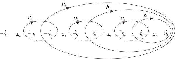
Figure 3: The Riemann surface $\mathcal{S}$ of genus three and its basis of circles.

The jump conditions for $g(\lambda)$ implies that for $j=1,2,3$

$$\oint_{a_{j}}\frac{\zeta^{4}+\alpha\zeta^{2}+\beta}{R_{+}(\zeta)}d\zeta=0,\ \oint_{b_{1}}\frac{\zeta^{4}+\alpha\zeta^{2}+\beta}{R_{+}(\zeta)}d\zeta=\Omega_{1},$$ (3.0.2)

$$\oint_{b_{2}}\frac{\zeta^{4}+\alpha\zeta^{2}+\beta}{R_{+}(\zeta)}d\zeta=\Omega_{0},\ \oint_{b_{3}}\frac{\zeta^{4}+\alpha\zeta^{2}+\beta}{R_{+}(\zeta)}d\zeta=\Omega_{2}.$$

Furthermore, it should be noted that $\frac{\zeta^{4}+\alpha\zeta^{2}+\beta}{R(\zeta)}d\zeta$, denoted as $\eta$, is a second kind Abelian differential on $\mathcal{S}$, with poles only at $\infty_{\pm}$. Introduce a basis of holomorphic differential as

$${\tilde{\omega}}_{j}=\frac{\zeta^{j-1}}{R(\zeta)}d\zeta,\quad j=1,2,3,$$

and denote $A:=(\oint_{a_{j}}\tilde{\omega}_{i})_{3\times 3}$ which is a non-degenerated matrix. According to the Reciprocity theorem [4], one can obtain that

$$\sum_{j=1}^{3}\oint_{a_{j}}\tilde{\omega}^{i}\oint_{b_{j}}\eta={2i\pi}\sum_{p=\infty_{\pm}}\mathrm{res}_{p}\frac{\tilde{\omega}_{i}}{\lambda},i=1,2,3,$$

that is,

$$\Omega_{1}\int_{a_{1}}\tilde{\omega}_{1}+\Omega_{0}\int_{a_{2}}\tilde{\omega}_{1}+\Omega_{2}\int_{a_{3}}\tilde{\omega}_{1}=0,$$ (3.0.3)

$$\Omega_{1}\int_{a_{1}}\tilde{\omega}_{2}+\Omega_{0}\int_{a_{2}}\tilde{\omega}_{2}+\Omega_{2}\int_{a_{3}}\tilde{\omega}_{2}=0,$$

$$\Omega_{1}\int_{a_{1}}\tilde{\omega}_{3}+\Omega_{0}\int_{a_{2}}\tilde{\omega}_{3}+\Omega_{2}\int_{a_{3}}\tilde{\omega}_{3}=4\pi i.$$

Consequently, the quantities $\Omega_{0}$, $\Omega_{1}$ and $\Omega_{2}$ can be expressed by

$$\Omega_{1}=4\pi i(A^{-1})_{13},\ \Omega_{0}=4\pi i(A^{-1})_{23},\ \Omega_{2}=4\pi i(A^{-1})_{33}.$$

Remark 3.1.

Since $\zeta/{R(\zeta)}$ is odd, and $1/{R(\zeta)}$ and $\zeta^{2}/{R(\zeta)}$ are even, it follows that $A_{13}=A_{11}$ and $A_{22}=0$, which implies that $(A^{-1})_{13}=(A^{-1})_{33}$, i.e., $\Omega_{1}=\Omega_{2}$. Alternatively, by using the equalities for $j=1,2$ below

$$\oint_{a_{j}}\frac{\zeta^{4}+\alpha\zeta^{2}+\beta}{R(\zeta)}d\zeta=0,$$

the parameters $\alpha$ and $\beta$ can be determined immediately.

Now, it is ready to deform the RH problem. To do so, take the transformation

$$T(\lambda)=Y(\lambda)e^{xg(\lambda)\sigma_{3}}f(\lambda)^{\sigma_{3}},$$

where $f(\lambda)$ is a function to be determined and $T(\lambda)$ satisfies the RH problem:

$$T_{+}(\lambda)=T_{-}(\lambda)V(\lambda)$$

$$V(\lambda)=\begin{cases}\begin{aligned} &\left(\begin{array}[]{cc}e^{x(g_{+}(\lambda)-g_{-}(\lambda))}\frac{f_{+}(\lambda)}{f_{-}(\lambda)}&\frac{-ir(\lambda)}{f_{+}(\lambda)f_{-}(\lambda)}\\ 0&e^{-x(g_{+}(\lambda)-g_{-}(\lambda))}\frac{f_{-}(\lambda)}{f_{+}(\lambda)}\end{array}\right),&\lambda\in\Sigma_{1,3},\\ &\left(\begin{array}[]{cc}e^{x(g_{+}(\lambda)-g_{-}(\lambda))}\frac{f_{+}(\lambda)}{f_{-}(\lambda)}&0\\ ir(\lambda)f_{+}(\lambda)f_{-}(\lambda)&e^{-x(g_{+}(\lambda)-g_{-}(\lambda))}\frac{f_{-}(\lambda)}{f_{+}(\lambda)}\end{array}\right),&\lambda\in\Sigma_{2,4},\\ &\left(\begin{array}[]{cc}e^{x\Omega_{0}}\frac{f_{+}(\lambda)}{f_{-}(\lambda)}&0\\ 0&e^{-x\Omega_{0}}\frac{f_{-}(\lambda)}{f_{+}(\lambda)}\end{array}\right),&\lambda\in\left[-\eta_{1},\eta_{1}\right],\\ &\left(\begin{array}[]{cc}e^{x\Omega_{1}}\frac{f_{+}(\lambda)}{f_{-}(\lambda)}&0\\ 0&e^{-x\Omega_{1}}\frac{f_{+}(\lambda)}{f_{-}(\lambda)}\end{array}\right),&\lambda\in[\eta_{2},\eta_{3}],\\ &\left(\begin{array}[]{cc}e^{x\Omega_{1}}\frac{f_{+}(\lambda)}{f_{-}(\lambda)}&0\\ 0&e^{-x\Omega_{1}}\frac{f_{+}(\lambda)}{f_{-}(\lambda)}\end{array}\right),&\lambda\in[-\eta_{3},-\eta_{2}],\end{aligned}\end{cases}$$

$$T(\lambda)=\left(\begin{array}[]{cc}1&1\end{array}\right)+\mathcal{O}\left(\frac{1}{\lambda}\right),\ \lambda\rightarrow\infty.$$

Moreover, the function $f(\lambda)$ can be established by the scalar RH problem:

$$f_{+}(\lambda)f_{-}(\lambda)={r(\lambda)}, \lambda\in\Sigma_{1,3},$$

$$f_{+}(\lambda)f_{-}(\lambda)=\frac{1}{r(\lambda)}, \lambda\in\Sigma_{2,4},$$

$$\frac{f_{+}(\lambda)}{f_{-}(\lambda)}=e^{\Delta_{0}}, \lambda\in[-\eta_{1},\eta_{1}],$$

$$\frac{f_{+}(\lambda)}{f_{-}(\lambda)}=e^{\Delta_{1}}, \lambda\in[\eta_{2},\eta_{3}],$$

$$\frac{f_{+}(\lambda)}{f_{-}(\lambda)}=e^{\Delta_{2}}, \lambda\in[-\eta_{3},-\eta_{2}],$$

$$f(\lambda)=1+\mathcal{O}\left(\frac{1}{\lambda}\right), \lambda\to\infty,$$

where $\Delta_{0}$, $\Delta_{1}$ and $\Delta_{2}$ are determined below. The Plemelj formula gives the solution of $f(\lambda)$ as

$$f(\lambda)= \exp\left(\frac{R(\lambda)}{2\pi i}\left[\int_{\Sigma_{1,3}}\frac{\log{r(\zeta)}}{R_{+}(\zeta)(\zeta-\lambda)}d\zeta+\int_{\Sigma_{2,4}}\frac{\log\frac{1}{r(\zeta)}}{R_{+}(\zeta)(\zeta-\lambda)}d\zeta+\int_{-\eta_{1}}^{\eta_{1}}\frac{\Delta_{0}}{R(\zeta)(\zeta-\lambda)}d\zeta\right.\right.$$ (3.0.4)

$$\left.\left.+\int_{\eta_{2}}^{\eta_{3}}\frac{\Delta_{1}}{R(\zeta)(\zeta-\lambda)}d\zeta+\int_{-\eta_{3}}^{-\eta_{2}}\frac{\Delta_{2}}{R(\zeta)(\zeta-\lambda)}d\zeta\right]\right).$$

Based on the boundary values of $f(\lambda)$, one can determine $\Delta_{0}$, $\Delta_{1}$ and $\Delta_{2}$ through the following system of linear algebraic equations:

$$\int_{\Sigma_{1,3}}\frac{\log{r(\zeta)}}{R_{+}(\zeta)}d\zeta+\int_{\Sigma_{2,4}}\frac{\log\frac{1}{r(\zeta)}}{R_{+}(\zeta)}d\zeta+\int_{-\eta_{1}}^{\eta_{1}}\frac{\Delta_{0}}{R(\zeta)}d\zeta+\int_{\eta_{2}}^{\eta_{3}}\frac{\Delta_{1}}{R(\zeta)}d\zeta+\int_{-\eta_{3}}^{-\eta_{2}}\frac{\Delta_{2}}{R(\zeta)}d\zeta=0,$$ (3.0.5)

$$\int_{\Sigma_{1,3}}\frac{\log{r(\zeta)}}{R_{+}(\zeta)}\zeta d\zeta+\int_{\Sigma_{2,4}}\frac{\log\frac{1}{r(\zeta)}}{R_{+}(\zeta)}\zeta d\zeta+\int_{-\eta_{1}}^{\eta_{1}}\frac{\Delta_{0}}{R(\zeta)}\zeta d\zeta+\int_{\eta_{2}}^{\eta_{3}}\frac{\Delta_{1}}{R(\zeta)}\zeta d\zeta+\int_{-\eta_{3}}^{-\eta_{2}}\frac{\Delta_{2}}{R(\zeta)}\zeta d\zeta=0,$$ (3.0.6)

$$\int_{\Sigma_{1,3}}\frac{\log{r(\zeta)}}{R_{+}(\zeta)}\zeta^{2}d\zeta+\int_{\Sigma_{2,4}}\frac{\log\frac{1}{r(\zeta)}}{R_{+}(\zeta)}\zeta^{2}d\zeta+\int_{-\eta_{1}}^{\eta_{1}}\frac{\Delta_{0}}{R(\zeta)}\zeta^{2}d\zeta+\int_{\eta_{2}}^{\eta_{3}}\frac{\Delta_{1}}{R(\zeta)}\zeta^{2}d\zeta+\int_{-\eta_{3}}^{-\eta_{2}}\frac{\Delta_{2}}{R(\zeta)}\zeta^{2}d\zeta=0.$$ (3.0.7)

Notice that $r(\zeta)$ is an even function, and $R_{+}(\zeta)$ has the opposite sign for $\zeta\in\Sigma_{1,3}$ compared to $\Sigma_{2,4}$. Thus, from the equation (3.0.6), it is deduced that $\Delta_{1}=\Delta_{2}$. Moreover, if expand the function $f(\lambda)$ for large $\lambda$, all involved terms are odd functions, which implies that $f(\lambda)$ tends to one as $\lambda$ approaches infinity.

Thus the jump matrix $V(\lambda)$ for $T(\lambda)$ is given by

$$V(\lambda)=\begin{cases}\begin{pmatrix}e^{x(g_{+}(\lambda)-g_{-}(\lambda))}\frac{f_{+}(\lambda)}{f_{-}(\lambda)}&-i\\ 0&e^{-x(g_{+}(\lambda)-g_{-}(\lambda))}\frac{f_{-}(\lambda)}{f_{+}(\lambda)}\end{pmatrix},&\lambda\in\Sigma_{1,3},\\ \begin{pmatrix}e^{x(g_{+}(\lambda)-g_{-}(\lambda))}\frac{f_{+}(\lambda)}{f_{-}(\lambda)}&0\\ i&e^{-x(g_{+}(\lambda)-g_{-}(\lambda))}\frac{f_{-}(\lambda)}{f_{+}(\lambda)}\end{pmatrix},&\lambda\in\Sigma_{2,4},\par\\ \begin{pmatrix}e^{x\Omega_{0}+\Delta_{0}}&0\\ 0&e^{-(x\Omega_{0}+\Delta_{0})}\end{pmatrix},&\lambda\in[-\eta_{1},\eta_{1}],\\ \begin{pmatrix}e^{x\Omega_{1}+\Delta_{1}}&0\\ 0&e^{-(x\Omega_{1}+\Delta_{1})}\end{pmatrix},&\lambda\in[\eta_{2},\eta_{3}]\cup[-\eta_{3},-\eta_{2}].\end{cases}$$ (3.0.8)

Now, define the analytic continuation $\hat{r}(\lambda)$ of $r(\lambda)$ off the interval $\Sigma_{1,2,3,4}$ with $\hat{r}_{\pm}(\lambda)=\pm r(\lambda)$ for $\lambda\in\Sigma_{1,2,3,4}$, and open lenses as follows

$$S(\lambda)=\begin{cases}T(\lambda)\begin{pmatrix}1&0\\ \frac{if^{2}(\lambda)}{\hat{r}(\lambda)}e^{2x(g(\lambda)-\lambda)}&1\end{pmatrix},&{\rm in~{}the~{}upper~{}lens,~{}above}~{}\Sigma_{1,3},\\ T(\lambda)\begin{pmatrix}1&0\\ \frac{if^{2}(\lambda)}{\hat{r}(\lambda)}e^{2x(g(\lambda)-\lambda)}&1\end{pmatrix},&{\rm in~{}the~{}lower~{}lens,~{}below}~{}\Sigma_{1,3},\\ T(\lambda)\begin{pmatrix}1&\frac{-i}{\hat{r}(\lambda)f^{2}(\lambda)}e^{-2x(g(\lambda)-\lambda)}\\ 0&1\end{pmatrix},&{\rm in~{}the~{}upper~{}lens,~{}above}~{}\Sigma_{2,4},\\ T(\lambda)\begin{pmatrix}1&\frac{-i}{\hat{r}(\lambda)f^{2}(\lambda)}e^{-2x(g(\lambda)-\lambda)}\\ 0&1\end{pmatrix},&{\rm in~{}the~{}lower~{}lens,~{}below}~{}\Sigma_{2,4},\\ T(\lambda),&{\rm outside~{}the~{}lenses}.\end{cases}$$ (3.0.9)

The vector-valued function $S(\lambda)$ satisfies the RH problem

$$S_{+}(\lambda) =S_{-}(\lambda)V_{S}(\lambda),$$ (3.0.10)

$$S(\lambda) =\begin{pmatrix}1&1\end{pmatrix}+O\left(\frac{1}{\lambda}\right),\quad\lambda\to\infty,$$

where the jump matrices $V_{S}(\lambda)$ are depicted in the Figure 4.

Figure 4: The jump contours for $S(\lambda)$ and the associated jump matrices: the gray terms in the matrices vanish exponentially as $x\to+\infty$, and the gray contours also vanish as $x\to+\infty$.

Lemma 3.2.

For $\lambda$ near $\Sigma_{1,3}\setminus\{\eta_{j}\}$ for $j=1,2,3,4$, the inequality $\operatorname{Re}(g(\lambda)-\lambda)<0$ holds. Conversely, for $\lambda$ near $\Sigma_{2,4}\setminus\{-\eta_{j}\}$, one has $\operatorname{Re}(g(\lambda)-\lambda)>0$.

It is noted that Lemma 3.2 is quite similar to the Lemma 4.6 and can be proven by the same way. So we omit the proof here for simplicity. Then for $x\to+\infty$, we arrive at the model problem $S^{\infty}(\lambda)$ as

$$S^{\infty}_{+}(\lambda)=S^{\infty}_{-}(\lambda)\begin{cases}\begin{pmatrix}0&-i\\ -i&0\end{pmatrix},&\lambda\in\Sigma_{1,3},\\ \begin{pmatrix}0&i\\ i&0\end{pmatrix},&\lambda\in\Sigma_{2,4},\\ \begin{pmatrix}e^{x\Omega_{0}+\Delta_{0}}&0\\ 0&e^{-x\Omega_{0}-\Delta_{0}}\end{pmatrix},&\lambda\in[-\eta_{1},\eta_{1}],\\ \begin{pmatrix}e^{x\Omega_{1}+\Delta_{1}}&0\\ 0&e^{-x\Omega_{1}-\Delta_{1}}\end{pmatrix},&\lambda\in[\eta_{2},\eta_{3}]\cup[-\eta_{3},-\eta_{2}],\end{cases}$$ (3.0.11)

where $S^{\infty}(\lambda)$ satisfies the boundary condition $S^{\infty}(\lambda)\to(1,1)$ as $\lambda\to\infty$ and the symmetry $S^{\infty}(-\lambda)=S^{\infty}(\lambda)\begin{pmatrix}0&1\\ 1&0\end{pmatrix}$, which serves as a generalization of the model problem discussed in [28]. Moreover, the model problem admits at most one quarter singularities at $\pm\eta_{1}$ and $\pm\eta_{3}$. In particular, the local parametrix near $\lambda=\pm\eta_{j}~{}(j=1,2,\dots,4)$ is expressed in terms of the modified Bessel functions under suitable conformal map [20].

3.1 The solution of the model RH problem on the $z$-plane

Now, transform the model RH problem (3.0.11) from the $\lambda$ plane into $z$ plane for $z=-\lambda^{2}$ by taking the upper half $\lambda$-plane onto $\mathbb{C}\setminus(-\infty,0)$. As a result, the model RH problem $S^{\infty}(\lambda)$ is converted into the RH problem on the $z$-plane, denoted as $S^{\infty}(z)$, which satisfies the following jump conditions

$$S^{\infty}_{+}(z)=S^{\infty}_{-}(z)\begin{cases}\begin{aligned} &\begin{pmatrix}0&e^{x\Omega_{0}+\Delta_{0}}\\ e^{-x\Omega_{0}-\Delta_{0}}&0\end{pmatrix},&&z\in[-\eta_{1}^{2},0],\\ &\begin{pmatrix}i&0\\ 0&i\end{pmatrix},&&z\in[-\eta_{2}^{2},-\eta_{1}^{2}]\cup[-\eta_{4}^{2},-\eta_{3}^{2}],\\ &\begin{pmatrix}0&e^{x\Omega_{1}+\Delta_{1}}\\ e^{-x\Omega_{1}-\Delta_{1}}&0\end{pmatrix},&&z\in[-\eta_{3}^{2},-\eta_{2}^{2}],\\ &\begin{pmatrix}0&1\\ 1&0\end{pmatrix},&&z\in[-\infty,-\eta_{4}^{2}].\\ \end{aligned}\end{cases}$$ (3.1.1)

Furthermore, $S^{\infty}(z)\to(1,1)$ as $z\to\infty$. The last jump matrix in the jump condition (3.1.1) is generated by the symmetry $S^{\infty}(-\lambda)=S^{\infty}(\lambda)\begin{pmatrix}0&1\\ 1&0\end{pmatrix}$, which also changes the diagonal jump matrices in the $\lambda$-plane into off-diagonal ones in the $z$-plane, see [32].

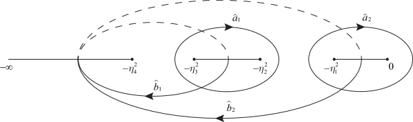
Figure 5: The Riemann surface $\hat{\mathcal{S}}$ and its basis $\{\hat{a}_{j},\hat{b}_{j}\},~{}j=1,2$ of circles.

Introduce the Riemann surface of genus two (see Figure 5) as

$$\hat{\mathcal{S}}:=\{(z,y)|y^{2}=z(z+\eta_{1}^{2})(z+\eta_{2}^{2})(z+\eta_{3}^{2})(z+\eta_{4}^{2})\},$$

and define the cycle basis $\{\hat{a}_{j},\hat{b}_{j}\}$ for $j=1,2$. Further, denote $\hat{R}(z)=\sqrt{z(z+\eta_{1}^{2})(z+\eta_{2}^{2})(z+\eta_{3}^{2})(z+\eta_{4}^{2})}$ and define the normalized holomorphic differential vector $\hat{\omega}=(\hat{\omega}_{1},\hat{\omega}_{2})^{T}$ such that $\oint_{a_{j}}\hat{\omega}_{k}=\delta_{jk}$ for $j=1,2$ where $\delta_{jk}=0$ and $1$ for $j\neq k$ and $j=k$ respectively. The associated period matrix $\hat{\tau}_{ij}=\oint_{\hat{b}_{j}}\hat{\omega}_{i}~{}(i,j=1,2)$ and $\hat{\tau}_{j}=\hat{\tau}e_{j}$, where $e_{j}$ is the $j$-th column of $2\times 2$ unit matrix for $j=1,2$. Thus the Abel map $\hat{J}(z)=\int_{\infty}^{z}\hat{\omega}$ has the following properties

$$\hat{J}_{+}(z)+\hat{J}_{-}(z)=0, z\in(-\infty,\eta_{4}^{2}],$$ (3.1.2)

$$\hat{J}_{+}(z)-\hat{J}_{-}(z)=-e_{1}-e_{2}, z\in[-\eta_{4}^{2},-\eta_{3}^{2}],$$

$$\hat{J}_{+}(z)+\hat{J}_{-}(z)=-\hat{\tau}_{1}, z\in[-\eta_{3}^{2},-\eta_{2}^{2}],$$

$$\hat{J}_{+}(z)-\hat{J}_{-}(z)=-e_{2}, z\in[-\eta_{2}^{2},-\eta_{1}^{2}],$$

$$\hat{J}_{+}(z)+\hat{J}_{-}(z)=-\hat{\tau}_{2}, z\in[-\eta_{1}^{2},0].$$

Introduce the Riemann-Theta function:

$$\Theta(z;\tau)=\sum_{\vec{n}\in\mathbb{Z}^{2}}e^{2\pi i\left(\vec{n}^{T}z+\frac{1}{2}\vec{n}^{T}\tau\vec{n}\right)},\quad z\in\mathbb{C}^{2},$$ (3.1.3)

which satisfies the following properties:

$$\Theta(z+e_{j};\hat{\tau})=\Theta(z-e_{j};\hat{\tau})=\Theta(z;\hat{\tau}),\quad\Theta(z+\hat{\tau}_{j};\hat{\tau})=e^{2\pi i(-z_{j}-\hat{\tau}_{jj}/2)}\Theta(z;\hat{\tau}),$$ (3.1.4)

Furthermore, define

$$\hat{\gamma}(z)=\left(\frac{(z+\eta_{1}^{2})(z+\eta_{3}^{2})}{(z+\eta_{2}^{2})(z+\eta_{4}^{2})}\right)^{\frac{1}{4}}.$$

Notice that the solution of model RH problem (3.1.1) on the $\lambda$-plane has at most one quarter singularities at $\pm\eta_{1}$ and $\pm\eta_{3}$, and this condition transforms into the solution of RH problem on the $z$-plane with singularities at $-\eta^{2}_{1}$ and $-\eta^{2}_{3}$ less than $1/4$. Furthermore, the zeros of $\hat{\gamma}(z)$ is $-\eta_{1}^{2}$ and $-\eta_{3}^{2}$ and the solution of the RH problem has the form

$$\frac{\Theta(\pm\hat{J}(z)-\frac{\Omega}{2\pi i}+\hat{d};\hat{\tau})}{\Theta(\pm\hat{J}(z)+\hat{d};\hat{\tau})},\quad\text{with}\quad\Omega=(x\Omega_{1}+\Delta_{1},x\Omega_{0}+\Delta_{0})^{T}.$$ (3.1.5)

It suffices to choose the parameter $\hat{d}$, which makes the zeros of denominator at $-\eta_{1}^{2}$ and $-\eta_{3}^{2}$, to nail down the singularities. On the other hand, we have

$$\hat{J}(\infty)=0,\ \hat{J}(-\eta_{4}^{2})=-\frac{e_{1}+e_{2}}{2},\ \hat{J}(-\eta_{3}^{2})=\frac{\hat{\tau}_{1}}{2}-\frac{e_{1}+e_{2}}{2},$$

$$\hat{J}(-\eta_{2}^{2})=\frac{\hat{\tau}_{1}}{2}-\frac{e_{2}}{2},\ \hat{J}(-\eta_{1}^{2})=\frac{\hat{\tau}_{2}}{2}-\frac{e_{2}}{2},\ \hat{J}(0)=\frac{\hat{\tau}_{1}}{2}.$$

The Riemann constant $\hat{\mathcal{K}}=\frac{\hat{\tau}_{1}+\hat{\tau}_{2}}{2}-\frac{e_{1}}{2}$, and further $\hat{J}(-\eta_{1}^{2})+\hat{J}(-\eta_{3}^{2})=\hat{\mathcal{K}}$, which implies $\hat{d}=0$. Consequently the solution of the model RH problem (3.1.1) on the $z$-plane is

$$\hat{S}^{\infty}(z)=\hat{\gamma}(z)\frac{\Theta(0;\hat{\tau})}{\Theta(\frac{\Omega}{2\pi i};\hat{\tau})}\left(\begin{array}[]{cc}\frac{\Theta(\hat{J}(z)-\frac{\Omega}{2\pi i};\hat{\tau})}{\Theta(\hat{J}(z);\hat{\tau})}&\frac{\Theta(-\hat{J}(z)-\frac{\Omega}{2\pi i};\hat{\tau})}{\Theta(-\hat{J}(z);\hat{\tau})}\end{array}\right).$$ (3.1.6)

In order to get the expansion of the Abel map $\hat{J}(z)$ as $z\to\infty$, we also need to transform the scalar RH problem for $g(\lambda)$ on the $\lambda$-plane into the case on the $z$-plane, that is

$$g_{+}(z)-g_{-}(z)=2i\sqrt{z}, z\in(-\eta_{4}^{2},-\eta_{3}^{2})\cup(-\eta_{2}^{2},-\eta_{1}^{2}),$$

$$g_{+}(z)+g_{-}(z)=0, z\in(-\infty,-\eta_{4}^{2}),$$

$$g_{+}(z)+g_{-}(z)=\Omega_{0}, z\in(-\eta_{1}^{2},0),$$

$$g_{+}(z)+g_{-}(z)=\Omega_{1}, z\in(-\eta_{3}^{2},-\eta_{2}^{2}),$$

$$g(z)=1+\mathcal{O}\left(\frac{1}{\sqrt{z}}\right), z\to\infty.$$

Consequently, the formula of $g(z)$ is

$$g(z)=\hat{R}(z)\left(\int_{-\eta_{3}^{2}}^{-\eta_{2}^{2}}\frac{\Omega_{1}}{\hat{R}(\mu)_{+}(\mu-z)}d\mu+\int_{-\eta_{1}^{2}}^{0}\frac{\Omega_{0}}{\hat{R}(\mu)_{+}(\mu-z)}d\mu+\left(\int_{-\eta_{4}^{2}}^{-\eta_{3}^{2}}+\int_{-\eta_{2}^{2}}^{-\eta_{1}^{2}}\right)\frac{2i\sqrt{\mu}}{\hat{R}(\mu)_{+}(\mu-z)}d\mu\right).$$

In order to keep consistence with the asymptotic condition, it follows that

$$\int_{\hat{a}_{1}}{\Omega_{1}}{\hat{\omega}_{j}}+\int_{\hat{a}_{2}}{\Omega_{0}}{\hat{\omega}_{j}}+4i\left(\int_{-\eta_{4}^{2}}^{-\eta_{3}^{2}}+\int_{-\eta_{2}^{2}}^{-\eta_{1}^{2}}\right)\sqrt{z}{\hat{\omega}_{j}}=0,\quad j=1,2,$$

and $4i\left(\int_{-\eta_{4}^{2}}^{-\eta_{3}^{2}}+\int_{-\eta_{2}^{2}}^{-\eta_{1}^{2}}\right)\sqrt{z}{\hat{\omega}_{j}}=2\pi\mathrm{res}_{\infty}\sqrt{z}{\hat{\omega}_{j}}$ for $j=1,2$, which indicates that $\mathrm{res}_{\infty}\sqrt{z}{\hat{\omega}}=-\frac{1}{2\pi}\begin{pmatrix}\Omega_{1}&\Omega_{0}\end{pmatrix}^{T}=-i\frac{\Omega_{x}}{2\pi i}$. As $z\to\infty$, expand $\hat{S}^{\infty}_{1}(z)$ as

$$\hat{S}^{\infty}_{1}(z)=1+\frac{\hat{S}^{\infty}_{11}}{z^{1/2}}+\mathcal{O}\left(\frac{1}{z}\right),$$

with

$$\hat{S}^{\infty}_{11}=-i\left[\nabla\log\left(\Theta\left(\frac{\Omega}{2\pi i}\right);\hat{\tau}\right)-\nabla\log(\Theta(0;\hat{\tau}))\right]\cdot\frac{\Omega_{x}}{2\pi i}.$$ (3.1.7)

Recall that $z=-\lambda^{2}$, hence the WKB expansion of solution $\hat{S}_{1}^{\infty}(z)$ on the parameter $\lambda$ is

$$\hat{S}^{\infty}_{1}(z)=1-\frac{1}{\lambda}\left[\nabla\log\left(\Theta\left(\frac{\Omega}{2\pi i}\right);\hat{\tau}\right)-\nabla\log(\Theta(0);\hat{\tau})\right]\cdot\frac{\Omega_{x}}{2\pi i}+\mathcal{O}\left(\frac{1}{\lambda^{2}}\right).$$ (3.1.8)

Here we choose $i\lambda$, since the map $\lambda\to z=-\lambda^{2}$ from the upper $\lambda$-plane to $\mathbb{C}\setminus{(-\infty,0)}$.

So far, we obtain the expression of $\hat{S}^{\infty}_{1}(z)$ and its expansion for $\lambda\to\infty$. To reconstruct the potential $u(x)$, one needs to concentrate on the error RH problem of $Y(\lambda)$ which in fact contributes the error term $\mathcal{O}(x^{-1})$ in the asymptotic behavior of $u(x)$ for $x\to+\infty$. The techniques for error estimation are illustrated in [20], although they differ slightly from those in this paper (see Remark 3.7).

Recall that the potential $u(x)$ can be recovered from the solution $Y(\lambda)$ as

$$u(x)=2\frac{\mathrm{d}}{\mathrm{d}x}\left[\lim_{\lambda\rightarrow\infty}{\lambda}\left(Y_{1}(\lambda;x)-1\right)\right].$$

After a series of transformations of the original RH problem, we have

$$Y_{1}(\lambda)=\left(\hat{S}_{1}^{\infty}(x;-\lambda^{2})+\frac{(\mathcal{E}_{1}(x))_{1}}{x\lambda}+\mathcal{O}\left(\frac{1}{\lambda^{2}}\right)\right)\frac{e^{-xg(\lambda)}}{f(\lambda)},$$

where $(\mathcal{E}_{1}(x))_{1}$ is the first entry of the vector $\mathcal{E}_{1}(x)$ given by equation (3.2.16). Moreover, reminding the expression of $g(\lambda)$ in (3.0.1), it follows

$$e^{-xg(\lambda)}=1-\frac{x}{\lambda}\left(\alpha+\frac{\eta_{1}^{2}+\eta_{2}^{2}+\eta_{3}^{2}+\eta_{4}^{2}}{2}\right)+\mathcal{O}\left(\frac{1}{\lambda^{2}}\right).$$ (3.1.9)

Similarly, from the formula of $f(\lambda)$, one has

$$f(\lambda)=1+\frac{f_{1}}{\lambda}+\mathcal{O}\left(\frac{1}{\lambda^{2}}\right),$$ (3.1.10)

where $f_{1}$ is independence of $x$. Consequently, combining (3.1.8), (3.1.9) with (3.1.10), it gives that

$$\small Y_{1}(\lambda)=1-\frac{1}{\lambda}\left(f_{1}+x\left(\alpha+\frac{\sum_{j=1}^{4}\eta_{j}^{2}}{2}\right)+\left(\nabla\log\left(\Theta\left(\frac{\Omega}{2\pi i}\right);\hat{\tau}\right)-\nabla\log(\Theta(0;\hat{\tau}))\right)\cdot\frac{\Omega_{x}}{2\pi i}+\frac{(\mathcal{E}_{1}(x))_{1}}{x}\right)+\mathcal{O}\left(\frac{1}{\lambda^{2}}\right),$$ (3.1.11)

which indicates that for $x\to+\infty$ the two-genus KdV soliton gas potential behaves

$$u(x)=-\left(2\alpha+{\sum_{j=1}^{4}\eta_{j}^{2}}+2\partial_{x}^{2}\log\left(\Theta\left(\frac{\Omega}{2\pi i};\hat{\tau}\right)\right)\right)+\mathcal{O}\left(\frac{1}{x}\right).$$ (3.1.12)

Remark 3.3.

In fact, one can also construct the solutions to the model RH problem (3.0.11) in the $\lambda$-plane, but through the $z$-plane, it is seen that the solution corresponding to the model problem is a Riemann surface $\hat{\mathcal{S}}$ of genus two rather than the Riemann surface $\mathcal{S}$ of genus three in the $\lambda$-plane. For the general Jacobi map on a Riemann surface of genus three, denoted by $J(\lambda)$, they are typically represented as a three-dimensional vector, with the corresponding Riemann-Theta function $\Theta(J(\lambda)-d)$ owning three zeros on the Riemann surface, while the function $\check{\gamma}(\lambda)=\left(\frac{(\lambda^{2}-\eta_{1}^{2})(\lambda^{2}-\eta_{3}^{2})}{(\lambda^{2}-\eta_{2}^{2})(\lambda^{2}-\eta_{4}^{2})}\right)^{\frac{1}{4}}$ has four zeros. Therefore, it is impossible to construct a vector model solution that satisfies the singularity requirements at the branch points $\pm\eta_{j},~{}j=1,2,3,4$.

Regarding the matrix solution of the model problem in Ref. [30], the authors there discussed a similar matrix model RH problem of by constructing the Riemann surface of genus one for the KdV equation, proving that there is no entire matrix solution for the aforementioned matrix model problem.

3.2 The solution of the model RH problem on the $\lambda$-plane

We have derived the solution of model RH problem $\hat{S}^{\infty}(z)$ on the $z$-plane; nevertheless, we also need to get the solution on $\lambda$-plane. Moreover, notice that the transformation $z=-\lambda^{2}$ can be considered as a holomorphic map between the Riemann surfaces $\mathcal{S}$ and $\hat{\mathcal{S}}$ in Figure 3 and Figure 5. In general, suppose that $\mathcal{S}$ is a Riemann surface of genus $2g-1$ for $g\in\mathbb{Z}_{+}$, i.e., $\mathcal{S}=\{(\lambda,y)|y^{2}=\Pi_{j=1}^{2g}(\lambda^{2}-\eta_{j}^{2})\},$ and Riemann surface $\hat{\mathcal{S}}$ on the $z$-plane, i.e., $\hat{\mathcal{S}}=\{(z,y)|y^{2}=z\Pi_{j=1}^{2g}(z+\eta_{j}^{2})\}$. Define the holomorphic map $\varphi:\mathcal{S}\to\hat{\mathcal{S}}$ with $-\lambda^{2}\to z$, and according to the Riemann-Hurwitz formula, it follows that the genus of Riemann surface $\hat{\mathcal{S}}$ is $g$. Indeed, we just transform the solution on the $z$-plane into $\lambda$-plane, especially, the normalized holomorphic differentials, basic cycles and period matrix. In the following, we will directly illustrate the model solution of $S^{\infty}(\lambda)$ and then develop the equivalence between the two solutions.

Similarly, define the normalized holomorphic differentials $\omega_{j}~{}(j=1,2,3)$ associated with Riemann surface $\mathcal{S}$ by $\omega=(\omega_{1},\omega_{2},\omega_{3})^{T}=A^{-1}\tilde{\omega}$, where $\tilde{\omega}=(\tilde{\omega}_{1},\tilde{\omega}_{2},\tilde{\omega}_{3})^{T}$ with $\tilde{\omega}_{j}=\frac{\zeta^{j-1}d\zeta}{R(\zeta)}~{}(j=1,2,3)$ and $A=(a_{ij})_{3\times 3}$ with $a_{ij}=\oint_{a_{j}}\tilde{\omega}_{i}$. Define the period matrix $\tau=(\tau_{ij})_{3\times 3}$ with $\tau_{ij}=\oint_{b_{j}}\omega_{i}$ and recall that the cycles are defined in Fig.3. Indeed, it follows from the parity of $\tilde{\omega}_{j}$ and the symmetries of $a$-cycles that $a_{11}=a_{13},a_{21}=-a_{23}$ and $a_{31}=a_{33}$. Moreover, it is straightforward to check that

$$\omega_{1}=A_{11}\tilde{\omega}_{1}+A_{12}\tilde{\omega}_{2}+A_{13}\tilde{\omega}_{3},\ \omega_{2}=A_{21}\tilde{\omega}_{1}+A_{23}\tilde{\omega}_{3},\ \omega_{3}=A_{11}\tilde{\omega}_{1}-A_{12}\tilde{\omega}_{2}+A_{13}\tilde{\omega}_{3},$$ (3.2.1)

where $A_{i,j}$ is the $(i,j)$ element of the matrix $A^{-1}$. It follows that $\omega_{1}+\omega_{3}$ and $2\omega_{2}$ have some nice symmetries on the Riemann surface $\mathcal{S}$ and the period matrix $\tau$ has the following properties:

$$\tau_{11}=\tau_{33},\tau_{12}=\tau_{23}.$$ (3.2.2)

Now, define the Jacobi map

$$\check{J}(\lambda)=\int_{\eta_{4}}^{\lambda}\check{\omega}:=\int_{\eta_{4}}^{\lambda}\begin{pmatrix}\omega_{1}+\omega_{3}\\ 2\omega_{2}\end{pmatrix},$$ (3.2.3)

and the corresponding period matrix is

$$\check{\tau}=\begin{pmatrix}\tau_{11}+\tau_{31}&\tau_{12}+\tau_{32}\\ 2\tau_{21}&2\tau_{22}\end{pmatrix}.$$ (3.2.4)

If one wants to use the above Jacobi map to construct the solution of model RH problem (3.0.11), it suffices to show that the imaginary part of $\check{\tau}$ is positive definite. In fact, it follows from the Riemann bilinear identity that $\tau_{ij}=\tau_{ji}$ and the properties of $\tau$ in (3.2.2) that $\check{\tau}$ is a principal minor of $\tau$ up to congruent transformations, which indicates that the imaginary part of $\check{\tau}$ is also positive definite. Consequently, the quotient space we choose is not $\mathbb{C}^{3}\setminus\{\tilde{e}_{j},\tau_{j}\}$ for $j=1,2,3$ but $\mathbb{C}^{2}\setminus\{e_{j},\check{\tau}_{j}\}$ for $j=1,2$, where $\tilde{e}_{j}$ is the $j$-th column of the $3\times 3$ identity matrix and $\check{\tau}_{j}$ is the $j$-th column of the matrix $\check{\tau}$. Indeed, we have

$$\oint_{b_{1}}\check{\omega}=\check{\tau}_{1},\ \oint_{b_{2}}\check{\omega}=\check{\tau}_{2},\ \oint_{b_{3}}\check{\omega}=\begin{pmatrix}\tau_{13}+\tau_{33}\\ 2\tau_{23}\end{pmatrix}=\check{\tau}_{1},$$ (3.2.5)

$$\oint_{a_{1}}\check{\omega}=e_{1},\ \oint_{a_{2}}\check{\omega}=2e_{2},\ \oint_{b_{3}}\check{\omega}=e_{1}.$$

Furthermore, it follows that the Jacobi map $\check{J}(z)$ satisfies

$$\check{J}_{+}(z)+\check{J}_{-}(z)=0, z\in\Sigma_{3},$$ (3.2.6)

$$\check{J}_{+}(z)+\check{J}_{-}(z)=-e_{1}, z\in\Sigma_{1},$$

$$\check{J}_{+}(z)+\check{J}_{-}(z)=-e_{1}-2e_{2}, z\in\Sigma_{2},$$

$$\check{J}_{+}(z)+\check{J}_{-}(z)=-2e_{1}-2e_{2}, z\in\Sigma_{4},$$

$$\check{J}_{+}(z)-\check{J}_{-}(z)=-\check{\tau}_{1}, z\in\left(\eta_{2},\eta_{3}\right),$$

$$\check{J}_{+}(z)-\check{J}_{-}(z)=-\check{\tau}_{2}, z\in\left(-\eta_{1},\eta_{1}\right),$$

$$\check{J}_{+}(z)-\check{J}_{-}(z)=-\check{\tau}_{1}, z\in\left(-\eta_{3},-\eta_{2}\right),$$

and the Jacobi map on the branch points are half periods, i.e.,

$$\check{J}(\eta_{4})=0,\ \check{J}(\eta_{3})=-\frac{\check{\tau}_{1}}{2},\ \check{J}(\eta_{2})=-\frac{\check{\tau}_{1}}{2}-\frac{e_{1}}{2},\ \check{J}(\eta_{1})=-\frac{\check{\tau}_{2}}{2}-\frac{e_{1}}{2},$$ (3.2.7)

$$\check{J}(-\eta_{4})=0,\ \check{J}(-\eta_{3})=-\frac{\check{\tau}_{1}}{2},\ \check{J}(-\eta_{2})=-\frac{\check{\tau}_{1}}{2}-\frac{e_{1}}{2},\ \check{J}(-\eta_{1})=-\frac{\check{\tau}_{2}}{2}-\frac{e_{1}}{2}.$$

On the other hand, based on the formula (3.2.3), for $\lambda\in\mathbb{C}\setminus\mathbb{R}$, one has

$$\check{J}(-\lambda)=\check{J}(\lambda)+e_{1}+e_{2},$$ (3.2.8)

which indicates that $\check{J}(\infty_{+})=\frac{e_{1}+e_{2}}{2}$. Now, the solution of the model RH problem for $S^{\infty}(\lambda)$ on the $\lambda$-plane can be written down. Initially, suppose that $\check{\gamma}(\lambda)=\left(\frac{(\lambda^{2}-\eta_{1}^{2})(\lambda^{2}-\eta_{3}^{2})}{(\lambda^{2}-\eta_{2}^{2})(\lambda^{2}-\eta_{4}^{2})}\right)^{\frac{1}{4}}$ and similarly assume that

$$S^{\infty}(\lambda)=\check{c}\check{\gamma}(\lambda)\begin{pmatrix}\frac{\Theta(\check{J}(\lambda)-\check{d}+\frac{\Omega}{2\pi i};\check{\tau})}{\Theta(\check{J}(\lambda)-\check{d};\check{\tau})}&\frac{\Theta(-\check{J}(\lambda)-\check{d}+\frac{\Omega}{2\pi i};\check{\tau})}{\Theta(-\check{J}(\lambda)-\check{d};\check{\tau})}\end{pmatrix},$$

where we demote the period matrix $\check{\tau}$ on the $\lambda$-plane comparing to $\hat{\tau}$ on the $z$-plane. In fact, it will be proven in the Lemma 3.9 that $\check{\tau}=\hat{\tau}$. Moreover, the parameters $\check{d}$ and $\check{c}$ should be determined. Note that we require the solution of RH problem on the $\lambda$-plane to have at most one quarter singularities at branch points $\pm\eta_{j}$ for $j=1,\cdots,4$, which implies that the zeros of $\Theta(\check{J}(\lambda)-\check{d};\check{\tau})$ and $\Theta(-\check{J}(\lambda)-\check{d};\check{\tau})$ both only lies at $\pm\eta_{1}$ and $\pm\eta_{3}$. Thus, it follows from the zeros of the Riemann-Theta function are odd half periods that $\check{d}=\frac{e_{1}+e_{2}}{2}$, and combining with $\check{J}(\infty_{+})=\frac{e_{1}+e_{2}}{2}$ shows that $\check{c}=\frac{\Theta(0;\check{\tau})}{\Theta(\frac{\Omega}{2\pi i};\check{\tau})}$. Recall that $\Omega=(x\Omega_{1}+\Delta_{1},x\Omega_{0}+\Delta_{0})^{T}$, thus $S^{\infty}(\lambda)$ exactly satisfies the jump conditions in (3.0.11). Now, we claim that the function $\Theta(\check{J}(\lambda))$ has precise four simple zeros on the Riemann surface $\mathcal{S}$, see [4].

Lemma 3.4.

For arbitrary fixed $d_{0}\in\mathbb{C}^{2}$, define the function $\vartheta(\lambda):\mathcal{S}\to\mathbb{C}$ with $\lambda\mapsto\Theta(\check{J}(\lambda)-d_{0};\check{\tau})$. We have $\deg(\vartheta)=4$, provided that $\vartheta$ does not vanish identically. Let $\mathcal{D}=(\vartheta)$, then $\check{J}(\mathcal{D})=d_{0}-\check{\mathcal{K}}$, with $\check{\mathcal{K}}_{k}=\frac{\check{\tau}_{kk}}{2}-\left(\oint_{a_{1}}\check{J}(\lambda)(\omega_{1}+\omega_{3})+\oint_{a_{2}}2\check{J}(\lambda)(\omega_{2})+\oint_{a_{3}}\check{J}(\lambda)(\omega_{1}+\omega_{3})\right)_{k},k=1,2$, where the subscript “$k$” denotes the $k$-th element of the column vector.

Proof.

Integrate $d\ln\vartheta$ along the boundary of the Riemann surface $\mathcal{S}$ denoted by $\delta\mathcal{S}$ as follows

$$\frac{1}{2\pi i}\oint_{\delta\mathcal{S}}\frac{d\vartheta(\lambda)}{\vartheta(\lambda)} =\frac{1}{2\pi i}\sum_{j=1}^{3}\left(\int_{\eta_{4}}^{\eta_{4}+a_{j}}+\int_{\eta_{4}+a_{j}}^{\eta_{4}+a_{j}+b_{j}}+\int_{\eta_{4}+a_{j}+b_{j}}^{\eta_{4}+b_{j}}+\int_{\eta_{4}+b_{j}}^{\eta_{4}}\right)d\ln\vartheta(\lambda)$$

$$=\frac{1}{2\pi i}\sum_{j=1}^{3}\left(\int_{\eta_{4}}^{\eta_{4}+a_{j}}-\int_{\eta_{4}+b_{j}}^{\eta_{4}+a_{j}+b_{j}}+\int_{\eta_{4}+b_{j}}^{\eta_{4}}-\int_{\eta_{4}+a_{j}+b_{j}}^{\eta_{4}+a_{j}}\right)d\ln\vartheta(\lambda)$$

$$=\int_{\eta_{4}}^{\eta_{4}+a_{1}}(\omega_{1}+\omega_{3})+\int_{\eta_{4}}^{\eta_{4}+a_{2}}2\omega_{2}+\int_{\eta_{4}}^{\eta_{4}+a_{3}}(\omega_{1}+\omega_{3})=4,$$

where we have used the fact that $d\ln\vartheta(\lambda+b_{1})=d\ln\vartheta(\lambda+b_{3})=-2\pi id(\check{J}(\lambda))_{1}+d\ln\vartheta(\lambda)$, $d\ln\vartheta(\lambda+b_{2})=-2\pi id(\check{J}(\lambda))_{2}+d\ln\vartheta(\lambda)$ and $d(\check{J}(\lambda))_{1}=\omega_{1}+\omega_{3},d(\check{J}(\lambda))_{2}=2\omega_{2}$. Similar to the above computation, integrate $\check{J}(\lambda)d\ln\vartheta(\lambda)$ along the boundary of Riemann surface $\delta\mathcal{S}$ in the following:

$$\frac{1}{2\pi i}\oint_{\delta\mathcal{S}}(\check{J}(\lambda))_{k}d\ln\vartheta(\lambda) =\frac{1}{2\pi i}\sum_{j=1}^{3}\left(\int_{\eta_{4}}^{\eta_{4}+a_{j}}+\int_{\eta_{4}+a_{j}}^{\eta_{4}+a_{j}+b_{j}}+\int_{\eta_{4}+a_{j}+b_{j}}^{\eta_{4}+b_{j}}+\int_{\eta_{4}+b_{j}}^{\eta_{4}}\right)(\check{J}(\lambda))_{k}d\ln\vartheta(\lambda)$$

$$=\frac{1}{2\pi i}\sum_{j=1}^{3}\left(\int_{\eta_{4}}^{\eta_{4}+a_{j}}-\int_{\eta_{4}+b_{j}}^{\eta_{4}+a_{j}+b_{j}}+\int_{\eta_{4}+b_{j}}^{\eta_{4}}-\int_{\eta_{4}+a_{j}+b_{j}}^{\eta_{4}+a_{j}}\right)(\check{J}(\lambda))_{k}d\ln\vartheta(\lambda)$$

$$=\frac{1}{2\pi i}\sum_{j=1}^{3}\int_{\eta_{4}}^{\eta_{4}+a_{j}}\left((\check{J}(\lambda))_{k}d\ln\vartheta(\lambda)-((\check{J}(\lambda))_{k}+\hat{\tau}_{kj})(d\ln\vartheta(\lambda)-2\pi id(\check{J}(\lambda))_{j})\right)$$

$$\quad+\frac{1}{2\pi i}\sum_{j=1}^{3}\int_{\eta_{4}}^{\eta_{4}+a_{j}}\left((\check{J}(\lambda))_{k}d\ln\vartheta(\lambda)-((\check{J}(\lambda))_{k}+2\pi i\delta_{jk})d\ln\vartheta(\lambda)\right)$$

$$=\oint_{a_{1}}(\check{J}(\lambda))_{k}(\omega_{1}+\omega_{3})+\oint_{a_{2}}2(\check{J}(\lambda))_{k}\omega_{2}+\oint_{a_{3}}(\check{J}(\lambda))_{k}(\omega_{1}+\omega_{3})-\frac{\hat{\tau}_{kk}}{2}+(d_{0})_{k}.$$

 

Finally, according to Lemma 3.4, it is immediate that both $\Theta(\check{J}(\lambda)-\check{d})$ and $\Theta(-\check{J}(\lambda)-\check{d})$ have four simple zeros, i.e., $\pm\eta_{1}$ and $\pm\eta_{3}$. So the solution to the model RH problem (3.0.11) is given by the following theorem.

Theorem 3.5.

Define $\check{J}(\lambda)=\int_{\eta_{4}}^{\lambda}\begin{pmatrix}\omega_{1}+\omega_{3}\\ 2\omega_{2}\end{pmatrix}$, where $\omega_{j}~{}(j=1,2,3)$ as defined previously are normalized holomorphic differentials on Riemann surface $\mathcal{S}$, then the corresponding period matrix $\check{\tau}$ is defined in (3.2.4), and let $\check{d}=\frac{e_{1}+e_{2}}{2},\Omega=\begin{pmatrix}x\Omega_{1}+\Delta_{1},x\Omega_{0}+\Delta_{0}\end{pmatrix}^{T}$, then the vector valued funtion

$$S^{\infty}(\lambda)=\check{\gamma}(\lambda)\frac{\Theta(0;\check{\tau})}{\Theta(\frac{\Omega}{2\pi i};\check{\tau})}\begin{pmatrix}\frac{\Theta(\check{J}(\lambda)-\check{d}+\frac{\Omega}{2\pi i};\check{\tau})}{\Theta(\check{J}(\lambda)-\check{d};\check{\tau})}&\frac{\Theta(-\check{J}(\lambda)-\check{d}+\frac{\Omega}{2\pi i};\check{\tau})}{\Theta(-\check{J}(\lambda)-\check{d};\check{\tau})}\end{pmatrix},$$ (3.2.9)

solves the RH problem (3.0.11).

Remark 3.6.

On the basis of calculation of $\Omega_{j}$, $j=0,1,2$ in (3.0.3), it implies that $\frac{\Omega}{2\pi i}$ is a real vector-valued function. Therefore, $S^{\infty}(\lambda)$ has no other singularities except for $\pm\eta_{1}$ and $\pm\eta_{3}$, since the zeros of the Riemann-Theta function is positioned at odd half periods.

Remark 3.7.

To finish the proof of Theorem 1.1, one should consider the error estimation of the potential $u(x)$ for $x\to+\infty$. However, to keep the length of the paper manageable, we omit this step since the detailed discussions are made in [20]. Still, it is necessary to introduce some notations to make our results complete.

Consider the $1$-form $dp=\frac{\lambda^{4}+\alpha\lambda^{2}+\beta}{R(\lambda)}d\lambda$ and the Abelian integral $p(\lambda)=\int_{\eta_{4}}^{\lambda}dp$, which satisfied

$$p_{+}(\lambda)+p_{-}(\lambda)=0, \lambda\in\Sigma_{1,2,3,4},$$ (3.2.10)

$$p_{+}(\lambda)-p_{-}(\lambda)=\Omega_{0}, \lambda\in[-\eta_{1},\eta_{1}],$$

$$p_{+}(\lambda)-p_{-}(\lambda)=\Omega_{1}, \lambda\in[-\eta_{3},-\eta_{2}]\cup[\eta_{2},\eta_{3}],$$

and

$$p(-\lambda)=-p(\lambda),\quad\lambda\in\mathbb{C}\setminus\mathbb{R}.$$ (3.2.11)

Further define

$$P^{\infty}(\lambda):=\frac{1}{2}\begin{pmatrix}(1+\frac{p(\lambda)}{\lambda})S_{1}^{\infty}+\frac{1}{\lambda}S_{1x}^{\infty}&(1-\frac{p(\lambda)}{\lambda})S_{2}^{\infty}+\frac{1}{\lambda}S_{2x}^{\infty}\\ (1-\frac{p(\lambda)}{\lambda})S_{1}^{\infty}-\frac{1}{\lambda}S_{1x}^{\infty}&(1+\frac{p(\lambda)}{\lambda})S_{2}^{\infty}-\frac{1}{\lambda}S_{2x}^{\infty}\end{pmatrix},$$ (3.2.12)

which satisfies the following matrix-valued RH problem with same jump matrices as $S^{\infty}(\lambda)$ and

$$P^{\infty}(\lambda)=\begin{pmatrix}1&0\\ 0&1\end{pmatrix}+\mathcal{O}\left(\frac{1}{\lambda}\right),\quad\lambda\to\infty,$$ (3.2.13)

$$P^{\infty}(\lambda){\rm~{}is~{}analytic~{}for~{}}\lambda\in\mathbb{C}\setminus[-\eta_{4},\eta_{4}]{\rm~{}with~{}a~{}singularity~{}at~{}}\lambda=0.$$

One can proof that $\det P^{\infty}(\lambda)\equiv 1$ for $\lambda\in\mathbb{C}$.

Now, let the solution of the error vector-valued RH problem defined by

$$\mathcal{E}(\lambda)=S(\lambda)(P(\lambda))^{-1},$$ (3.2.14)

where the global parametrix $P(\lambda)$ is given by

$$P(\lambda)=\begin{cases}P^{\infty}(\lambda),&\lambda\in\mathbb{C}\setminus\cup_{j=1,2,3,4}B_{\rho}^{\pm\eta_{j}},\\ P^{\diamond}(\lambda),&\lambda\in B_{\rho}^{\diamond},\end{cases}$$ (3.2.15)

where $\diamond$ traverses all $8$ branch points, i.e., $\pm\eta_{j}$, $j=1,2,3,4$ and $B_{\rho}^{\diamond}$ denotes the open disc of radius $\rho$ centered at $\diamond$. We claim that the local parametrix $P^{\pm\eta_{j}}$ near $\lambda=\pm\eta_{j}$, $j=1,2,3,4$ can be described by the modified Bessel function which will finally contribute the term $\mathcal{O}(x^{-1})$ in the asymptotic result of $u(x)$ for $x\to+\infty$.

Therefore, one can see that

$$Y(\lambda)=\mathcal{E}(\lambda)P(\lambda)e^{-xg(\lambda)\sigma_{3}}f(\lambda)^{-\sigma_{3}}=\left(\begin{pmatrix}1&1\end{pmatrix}+\frac{\mathcal{E}_{1}(x)}{x\lambda}+\mathcal{O}\left(\frac{1}{\lambda^{2}}\right)\right)P(\lambda)e^{-xg(\lambda)\sigma_{3}}f(\lambda)^{-\sigma_{3}}.$$ (3.2.16)

Recall that the potential $u(x)$ can be reconstructed from the solution of $Y(\lambda)$ as following

$$u(x)=2\frac{\mathrm{d}}{\mathrm{d}x}\left[\lim_{\lambda\rightarrow\infty}{\lambda}\left(Y_{1}(\lambda;x)-1\right)\right].$$

Theorem 3.8.

As $x\to+\infty$, the potential $u(x)$ is subject to the following asymptotic expression

$$u(x)=-\left(2\alpha+{\sum_{j=1}^{4}\eta_{j}^{2}}+2\partial_{x}^{2}\log\left(\Theta\left(\frac{\Omega}{2\pi i};\check{\tau}\right)\right)\right)+\mathcal{O}\left(\frac{1}{x}\right),$$ (3.2.17)

where $\alpha$ is associated to a second kind Abel differential and can be calculated in remark (3.1).

Proof.

Similarly,

$$Y_{1}(\lambda)=\left(S_{1}^{\infty}(x;\lambda)+\frac{(\mathcal{E}_{1}(x))_{1}}{x\lambda}+\mathcal{O}\left(\frac{1}{\lambda^{2}}\right)\right)\frac{e^{-xg(\lambda)}}{f(\lambda)},$$

where $(\mathcal{E}_{1}(x))_{1}$ is the first entry of the vector $\mathcal{E}_{1}(x)$ given by equation (3.2.16). Recall that

$$e^{-xg(\lambda)}=1-\frac{x}{\lambda}\left(\alpha+\frac{\eta_{1}^{2}+\eta_{2}^{2}+\eta_{3}^{2}+\eta_{4}^{2}}{2}\right)+\mathcal{O}\left(\frac{1}{\lambda^{2}}\right),$$

and

$$f(\lambda)=1+\frac{f_{1}}{\lambda}+\mathcal{O}\left(\frac{1}{\lambda^{2}}\right).$$

In addition, recall the linear equations (3.0.3), and change $\tilde{\omega}_{j}$ into $\omega_{j}~{}(j=1,2,3)$, it follows from the Reciprocity theorem [4] that

$$2\pi i\ \sum\mathrm{res}_{\infty_{\pm}}\frac{\omega_{1}}{z}=\Omega_{1},\ 2\pi i\ \sum\mathrm{res}_{\infty_{\pm}}\frac{\omega_{2}}{z}=\Omega_{2},\ 2\pi i\ \sum\mathrm{res}_{\infty_{\pm}}\frac{\omega_{3}}{z}=\Omega_{1}.$$

Incorporate with the symmetry in (3.2.8), which implies that as $\lambda\to\infty$

$$J(\lambda)=\frac{e_{1}+e_{2}}{2}-\frac{\Omega_{x}}{\lambda}+\mathcal{O}\left(\frac{1}{\lambda^{2}}\right).$$

Moreover, the expanding of $S_{1}^{\infty}(\lambda)$ as $\lambda\to\infty$ is

$${S}^{\infty}_{1}(\lambda) =1-\frac{1}{\lambda}\left[\nabla\log\left(\Theta\left(\frac{\Omega}{2\pi i};\check{\tau}\right)\right)-\nabla\log(\Theta(0;\check{\tau}))\right]\cdot\frac{\Omega_{x}}{2\pi i}+\mathcal{O}\left(\frac{1}{\lambda^{2}}\right),$$

$$=1-\frac{1}{\lambda}\partial_{x}\log\left(\Theta\left(\frac{\Omega}{2\pi i};\check{\tau}\right)\right)+\mathcal{O}\left(\frac{1}{\lambda^{2}}\right).$$

Thus,

$$Y_{1}(\lambda)=1-\frac{1}{\lambda}\left[f_{1}+x\left(\alpha+\frac{1}{2}\sum_{j=1}^{4}\eta_{j}^{2}\right)+\partial_{x}\log\left(\Theta\left(\frac{\Omega}{2\pi i};\check{\tau}\right)\right)+\frac{(\mathcal{E}_{1}(x))_{1}}{x}\right]+\mathcal{O}\left(\frac{1}{\lambda^{2}}\right).$$

Consequently, based on the relationship between $u(x)$ and $Y(\lambda)$, we have

$$u(x)=-\left(2\alpha+{\sum_{j=1}^{4}\eta_{j}^{2}}+2\partial_{x}^{2}\log\left(\Theta\left(\frac{\Omega}{2\pi i};\check{\tau}\right)\right)\right)+\mathcal{O}\left(\frac{1}{x}\right).$$

 

So far, we almost complete the construction of the soliton gas potential in the regime $x\to+\infty$. However, there is a minor flaw, which lies in proving the equivalence of the period matrices $\check{\tau}$ and $\hat{\tau}$.

Lemma 3.9.

Suppose that $\omega_{j}$, $j=1,2,3$ defined previously are the normalized holomorphic differentials on Riemann surface $\mathcal{S}$, and then $\omega_{1}+\omega_{3},2\omega_{2}$ are the normalized holomorphic differentials on the transformed Riemann surface $\hat{\mathcal{S}}$. Moreover, the period matrix $\check{\tau}$ is precisely $\hat{\tau}$.

Proof.

Recalling the definition of $\tilde{\omega}_{j}$ and changing the variable $\lambda$ into $i\sqrt{z}$, we have the following local expressions

$$\tilde{\omega}_{1}=\frac{d\lambda}{R(\lambda)}=\frac{i}{2}\frac{dz}{\hat{R}(z)},\ \tilde{\omega}_{2}=\frac{\lambda d\lambda}{R(\lambda)}=-\frac{1}{2}\frac{\sqrt{z}dz}{\hat{R}(z)},\ \tilde{\omega}_{3}=\frac{\lambda^{2}d\lambda}{R(\lambda)}=-\frac{i}{2}\frac{zdz}{\hat{R}(z)}.$$

It follows that after the holomorphic transformation $z=-\lambda^{2}$, the original holomorphic differential $\tilde{\omega}_{2}$ is not a holomorphic differential in $\hat{\mathcal{S}}$. Fortunately, by the expressions of $\omega_{j}$ in terms of $\tilde{\omega}_{j}$ in (3.2.1), $\omega_{1}+\omega_{2}$ and $2\omega_{2}$ are irrelated to $\tilde{\omega}_{2}$. In particular,

$$\oint_{\hat{a}_{1}}(\omega_{1}+\omega_{3})\rvert_{\hat{\mathcal{S}}}=\oint_{a_{1}}(\omega_{1}+\omega_{3})\rvert_{\mathcal{S}}=\oint_{a_{3}}(\omega_{1}+\omega_{3})\rvert_{\mathcal{S}}=1,\quad\oint_{\hat{a}_{2}}2\omega_{2}\rvert_{\hat{\mathcal{S}}}=\oint_{a_{2}}\omega_{2}\rvert_{\mathcal{S}}=1,$$

$$\oint_{\hat{a}_{1}}2\omega_{2}\rvert_{\hat{\mathcal{S}}}=\oint_{a_{1}}2\omega_{2}\rvert_{\mathcal{S}}=\oint_{a_{3}}2\omega_{2}\rvert_{\mathcal{S}}=0,\quad\oint_{\hat{a}_{2}}(\omega_{1}+\omega_{3})\rvert_{\hat{\mathcal{S}}}=\frac{1}{2}\oint_{a_{1}}(\omega_{1}+\omega_{3})\rvert_{\mathcal{S}}=0.$$

By the Riemann Bilinear relationship, it indicates that $(\omega_{1}+\omega_{3})\rvert_{\hat{\mathcal{S}}}$ and $2\omega_{2}\rvert_{\hat{\mathcal{S}}}$ are the normalized holomorphic differentials on $\hat{\mathcal{S}}$ and the corresponding period matrix are equivalence.   

3.3 Behavior of the two-genus KdV soliton gas potential for $x\to-\infty$

The behavior of the two-genus KdV soliton gas potential is quite simple since the jump matrices of the RH problem $Y(\lambda)$ are all converge to identity matrix exponentially when $x\to-\infty$. To be precise, there exist a fixed constant $c\in\mathbb{R}_{+}$ such that for $x\to-\infty$, the boundary behavior of the potential $u(x)$ is given by

$$u(x)=\mathcal{O}(e^{-c|x|}).$$ (3.3.1)

4 Evolution of the two-genus KdV soliton gas potential for $t\to+\infty$

This section examines the large-time asymptotic behaviors of the two-genus KdV soliton gas potential constructed in Section 2 and presents a detailed proof of the Theorem 1.2.

If the two-genus KdV soliton gas potential $u(x,0)$ evolves in time according to the KdV equation, the reflection coefficient $r(t;\lambda)=r(\lambda)e^{-8\lambda^{3}t}$. It follows that the RH problem of $Y(\lambda)=Y(\lambda;x,t)$ for the evolution of soliton gas is defined by

$$Y_{+}(\lambda)=Y_{-}(\lambda)\begin{cases}{\left(\begin{array}[]{cc}1&-ir(\lambda)e^{2\lambda x-8\lambda^{3}t}\\ 0&1\end{array}\right)},&\lambda\in\Sigma_{1,3},\\ {\left(\begin{array}[]{cc}1&0\\ ir(\lambda)e^{-2\lambda x+8\lambda^{3}t}&1\end{array}\right)},&\lambda\in\Sigma_{2,4},\end{cases}$$ (4.0.1)

with the same boundary condition and symmetry in accordance with the case of the initial soliton gas potential, i.e., $Y(\lambda)=(1\quad 1)+\mathcal{O}\left(\frac{1}{\lambda}\right),$ and $Y(-\lambda)=Y(\lambda)\left(\begin{matrix}0&1\\ 1&0\end{matrix}\right)$, respectively. In order to analyze the asymptotic behavior of $Y(x,t;\lambda)$ in the long time sense, rewrite the phase function $2\lambda x-8\lambda^{3}t=8\lambda t(\xi-\lambda^{2})$ with $\xi=\frac{x}{4t}\in\mathbb{R}$.

It is immediate that in the case $\xi<\eta_{1}^{2}$, the phase functions in the jump matrices are exponentially decreasing as $t\to+\infty$. Consequently, straightforward calculation shows that

$$Y(\lambda)=(1\quad 1)+\mathcal{O}\left(e^{8\eta_{1}t(\xi-\eta_{1}^{2})}\right),$$

as $t\to+\infty$ with $\xi<\eta_{1}^{2}$, which indicates that the potential $u(x,t)$ vanishes rapidly in this region.

4.1 Modulated one-phase wave region

Introduce the critical value $\xi_{crit}^{(1)}$ that is defined by (4.1.10) below, and consider the constraint

$$\eta_{1}^{2}<\xi<\xi_{crit}^{(1)}.$$

Split the contours in $\Sigma_{1,2}$ in such ways

$$\Sigma_{1_{\alpha_{1}}}=(\eta_{1},\alpha_{1})\ \text{and}\ \Sigma_{2_{\alpha_{1}}}=(-\alpha_{1},-\eta_{1}),$$ (4.1.1)

where the $\alpha_{1}$ will be determined in (4.1.8) as a function of $\xi$. Similarly, introduce the $g$ function, denoted as $g_{\alpha_{1}}$, which satisfies the following scalar RH problem:

$$g_{\alpha_{1,+}}(\lambda)+g_{\alpha_{1,-}}(\lambda)+8\lambda^{3}-8\xi\lambda=0, \lambda\in\Sigma_{1_{\alpha_{1}}}\cup\Sigma_{2_{\alpha_{1}}},$$ (4.1.2)

$$g_{\alpha_{1,+}}(\lambda)-g_{\alpha_{1,-}}(\lambda)={\Omega_{\alpha_{1}}}, \lambda\in[-\eta_{1},\eta_{1}],$$

$$g_{\alpha_{1}}(\lambda)=\mathcal{O}\left(\frac{1}{\lambda}\right), \lambda\to\infty.$$

To further deform the RH problem (4.0.1), it is required that the $g_{\alpha_{1}}$ function satisfies the following properties:

$$g_{\alpha_{1}}(\lambda)+4\lambda^{3}-4\xi\lambda=(\lambda\pm\alpha_{1})^{\frac{3}{2}}, \lambda\to\pm\alpha_{1},$$ (4.1.3)

$$\operatorname{Re}\left(g_{\alpha_{1}}(\lambda)+4\lambda^{3}-4\xi\lambda\right)>0, \lambda\in(\alpha_{1},\eta_{2})\cup\Sigma_{3},$$

$$\operatorname{Re}\left(g_{\alpha_{1}}(\lambda)+4\lambda^{3}-4\xi\lambda\right)<0, \lambda\in(-\eta_{2},-\alpha_{1})\cup\Sigma_{4},$$

$$-i(g_{\alpha_{1},+}(\lambda)-g_{\alpha_{1},-}(\lambda))\text{ is real-valued and monotonically increasing}, \lambda\in\Sigma_{1_{\alpha_{1}}},$$

$$-i(g_{\alpha_{1},+}(\lambda)-g_{\alpha_{1},-}(\lambda))\text{ is real-valued and monotonically decreasing}, \lambda\in\Sigma_{2_{\alpha_{1}}}.$$

The $g_{\alpha_{1}}$ can be derived from its derivative $g^{\prime}_{\alpha_{1}}$ according to the uniqueness of $g_{\alpha_{1}}$. Here the $g^{\prime}_{\alpha_{1}}d\lambda$ can be viewed as the second kind Abel differential on Riemann surface of genus one.

Define

$$g^{\prime}_{\alpha_{1}}(\lambda)=-12\lambda^{2}+4\xi+12\frac{Q_{\alpha_{1},2}(\lambda)}{R_{\alpha_{1}}(\lambda)}-4\xi\frac{Q_{\alpha_{1},1}(\lambda)}{R_{\alpha_{1}}(\lambda)},$$ (4.1.4)

with

$$R_{\alpha_{1}}(\lambda)=\sqrt{(\lambda^{2}-\eta_{1}^{2})(\lambda^{2}-\alpha_{1}^{2})},$$

which is analytic for $\mathbb{C}\setminus\left(\Sigma_{1_{\alpha_{1}}}\cup\Sigma_{2_{\alpha_{1}}}\right)$, and takes positive real value for $\lambda>\alpha_{1}$. From the definition of $g_{\alpha_{1}}^{\prime}(\lambda)$ in (4.1.4), we can derive the expression of $g_{\alpha_{1}}(\lambda)$:

$$g_{\alpha_{1}}(\lambda)=-4\lambda^{3}+4\xi\lambda+12\int_{\alpha_{1}}^{\lambda}\frac{Q_{\alpha_{1},2}(\zeta)}{R_{\alpha_{1}}(\zeta)}d\zeta-4\xi\int_{\alpha_{1}}^{\lambda}\frac{Q_{\alpha_{1},1}(\zeta)}{R_{\alpha_{1}}(\zeta)}d\zeta.$$ (4.1.5)

On the other hand, suppose that

$$Q_{\alpha_{1},1}(\lambda)=\lambda^{2}+c_{\alpha_{1},1},\quad Q_{\alpha_{1},2}(\lambda)=\lambda^{4}-\frac{1}{2}(\alpha_{1}^{2}+\eta_{1}^{2})\lambda^{2}+c_{\alpha_{1},2},$$ (4.1.6)

where

$$c_{\alpha_{1},1}=-\alpha_{1}^{2}+\alpha_{1}^{2}\frac{E(m_{\alpha_{1}})}{K(m_{\alpha_{1}})},\quad c_{\alpha_{1},2}=\frac{1}{3}\alpha_{1}^{2}\eta_{1}^{2}+\frac{1}{6}(\alpha_{1}^{2}+\eta_{1}^{2})c_{\alpha_{1},1},\quad m_{\alpha_{1}}=\frac{\eta_{1}}{\alpha_{1}}.$$ (4.1.7)

Here $K(m_{\alpha_{1}})$ and $E(m_{\alpha_{1}})$ are the first and the second kind complete elliptic integral, respectively, i.e., $K(m)=\int_{0}^{\frac{\pi}{2}}\frac{d\vartheta}{\sqrt{1-m^{2}\sin\vartheta^{2}}}$ and $E(m)=\int_{0}^{\frac{\pi}{2}}{\sqrt{1-m^{2}\sin\vartheta^{2}}}{d\vartheta}$. The $Q_{\alpha_{1},1}$ and $Q_{\alpha_{1},2}$ are determined by the conditions in (4.1.2), and the first property in (4.1.3) about the behavior near $\pm\alpha_{1}$ implies that the parameter $\alpha_{1}$ is determined by

$$\xi=3\frac{Q_{\alpha_{1},2}(\pm\alpha_{1})}{Q_{\alpha_{1},1}(\pm\alpha_{1})}=\frac{1}{2}(\alpha_{1}^{2}+\eta_{1}^{2})+(\alpha_{1}^{2}-\eta_{1}^{2})\frac{K(m_{\alpha_{1}})}{E(m_{\alpha_{1}})},$$ (4.1.8)

which states that the $\alpha_{1}$ is modulated by $\xi$. Indeed, rewrite (4.1.8) as Whitham velocity

$$\xi=\frac{x}{4t}=\frac{\eta_{1}^{2}}{2}\left[1+\frac{1}{m_{\alpha_{1}}^{2}}+\left(\frac{1}{m_{\alpha_{1}}^{2}}-1\right)\frac{K(m_{\alpha_{1}})}{E(m_{\alpha_{1}})}\right]:=\frac{\eta_{1}^{2}}{2}W(m_{\alpha_{1}}).$$ (4.1.9)

It follows that $\partial_{\alpha_{1}}W(m_{\alpha_{1}})>0$ for $\eta_{1}<\alpha_{1}<+\infty$, since the Whitham equation associated with the Whitham velocity (4.1.9) is strictly hyperbolic. In fact, direct calculation also shows that $\partial_{m_{\alpha_{1}}}W(m_{\alpha_{1}})<0$ for $0<m_{\alpha_{1}}<1$. According to the expansions of elliptic functions, it is immediate that

$$\lim_{\alpha\to\eta_{1}}\xi=\eta_{1}^{2},\ m_{\alpha_{1}}\to 1,\ \text{and}\ \lim_{\alpha\to+\infty}\xi=+\infty,\ m_{\alpha_{1}}\to 0.$$

Define

$$\xi_{crit}^{(1)}:=3\frac{Q_{\alpha_{1},2}(\eta_{2})}{Q_{\alpha_{1},1}(\eta_{2})}=\frac{1}{2}(\eta_{1}^{2}+\eta_{2}^{2})+(\eta_{2}^{2}-\eta_{1}^{2})\frac{K(m_{\eta_{2}})}{E(m_{\eta_{2}})},$$ (4.1.10)

where $m_{\eta_{2}}=\frac{\eta_{1}}{\eta_{2}}$. Consequently, (4.1.8) defines $\alpha_{1}$ as a monotone increasing function of $\xi$ in $[\eta_{1}^{2},\xi_{crit}^{(1)}]$ by the implicit function theorem. If the relationship (4.1.8) is established, we can verify the first condition in (4.1.3). Indeed, together with (4.1.7), rewrite the function $g^{\prime}_{\alpha_{1}}(\lambda)$ as

$$g^{\prime}_{\alpha_{1}}(\lambda) =-12\lambda^{2}+4\xi+12\frac{Q_{\alpha_{1},2}(\lambda)-Q_{\alpha_{1},2}(\alpha_{1})}{R_{\alpha_{1}}(\lambda)}-4\xi\frac{Q_{\alpha_{1},1}(\lambda)-Q_{\alpha_{1},1}(\alpha_{1})}{R_{\alpha_{1}}(\lambda)}$$

$$=-12\lambda^{2}+4\xi+12\frac{(\lambda^{2}-\alpha_{1}^{2})}{R_{\alpha_{1}}(\lambda)}\left[\lambda^{2}-\left(\frac{\eta_{1}^{2}-\alpha_{1}^{2}}{2}+\frac{\xi}{3}\right)\right].$$

It follows that $g^{\prime}_{\alpha_{1}}(\lambda)$ behaves like $(\lambda\pm\alpha_{1})^{\frac{1}{2}}$ as $\lambda\to\pm\alpha_{1}$, and $(\lambda\pm\eta_{1})^{-\frac{1}{2}}$ as $\lambda\to\pm\eta_{1}$, which is coincided with (4.1.3). Before verifying the other conditions in (4.1.3), we will determine ${\Omega}_{\alpha_{1}}$ in the jump condition (4.1.2) and introduce the following Riemann surface of genus one related to $R_{\alpha_{1}}(\lambda)$:

$$\mathcal{S}_{\alpha_{1}}:=\{(\lambda,\eta)|\eta^{2}=(\lambda^{2}-\eta_{1}^{2})(\lambda^{2}-\alpha_{1}^{2})\},$$

with the $A$, $B$-cycles defined in Figure 6. Define

$$\omega_{\alpha_{1}}=-\frac{\alpha_{1}d\zeta}{4K(m_{\alpha_{1}})R_{\alpha_{1}}(\zeta)},$$

as the normalized holomorphic differential on $\mathcal{S}_{\alpha_{1}}$ with $\oint_{A}\omega_{\alpha_{1}}=1$ and $\oint_{B}\omega_{\alpha_{1}}=\tau_{\alpha_{1}}$. Reminding the definition of $g_{\alpha_{1}}(\lambda)$ and jump conditions in (4.1.2), it implies that

$$24\int_{\alpha_{1}}^{\eta_{1}}\frac{Q_{\alpha_{1},2}(\zeta)}{R_{\alpha_{1}}(\zeta)}d\zeta-8\xi\int_{\alpha_{1}}^{\eta_{1}}\frac{Q_{\alpha_{1},1}(\zeta)}{R_{\alpha_{1}}(\zeta)}d\zeta={\Omega}_{\alpha_{1}},$$ (4.1.11)

$$\int_{-\eta_{1}}^{\eta_{1}}\frac{Q_{\alpha_{1},2}(\zeta)}{R_{\alpha_{1}}(\zeta)}d\zeta=\int_{-\eta_{1}}^{\eta_{1}}\frac{Q_{\alpha_{1},1}(\zeta)}{R_{\alpha_{1}}(\zeta)}d\zeta=0.$$

In fact, $\frac{Q_{\alpha_{1},2}(\lambda)}{R_{\alpha_{1}}(\lambda)}d\lambda$ and $\frac{Q_{\alpha_{1},1}(\lambda)}{R_{\alpha_{1}}(\lambda)}d\lambda$ are the normalized Abel differentials of the second kind and by using the Reciprocity theorem [4], it follows from (4.1.11) that

$${\Omega}_{\alpha_{1}} =-12\int_{B}\frac{Q_{\alpha_{1},2}(\zeta)}{R_{\alpha_{1}}(\zeta)}d\zeta+4\xi\int_{B}\frac{Q_{\alpha_{1},1}(\zeta)}{R_{\alpha_{1}}(\zeta)}d\zeta$$ (4.1.12)

$$=2\pi i(4\xi\mathrm{res}_{\lambda=\pm\infty}\lambda^{-1}\omega_{\alpha_{1}}-4\mathrm{res}_{\lambda=\pm\infty}\lambda^{-3}\omega_{\alpha_{1}})=2\pi i\alpha_{1}\frac{\alpha_{1}^{2}+\eta_{1}^{2}-2\xi}{K(m_{\alpha_{1}})}\in i\mathbb{R}.$$

\begin{overpic}[width=303.53267pt]{genus1.png} \put(43.3,27.0){ A} \put(72.3,29.3){ B} \put(32.3,13.3){ $-\eta_{1}$} \put(62.3,13.3){ $\eta_{1}$} \put(3.0,13.3){ $-\alpha_{1}$} \put(91.3,13.3){ $\alpha_{1}$} \end{overpic}

Figure 6: The Riemann surface $\mathcal{S}_{\alpha_{1}}$ of genus one and its basis of cycles

In order to recover the potential function $u(x,t)$, it is necessary to formulate $\partial_{x}(tg^{\prime}_{\alpha_{1}}(\lambda))$ and $\partial_{x}(t{\Omega}_{\alpha_{1}})$. Thus we have the following lemma.

Lemma 4.1.

According the representation of $g^{\prime}_{\alpha_{1}}(\lambda)$ in (4.1.4) and ${\Omega}_{\alpha_{1}}$ in (4.1.11), the following two identities hold

$$\partial_{x}(tg^{\prime}_{\alpha_{1}}(\lambda))=1-\frac{Q_{\alpha_{1},1}(\lambda)}{R_{\alpha_{1}}(\lambda)},$$ (4.1.13)

$$\partial_{x}(t{\Omega}_{\alpha_{1}})=-\frac{\pi i\alpha_{1}}{K(m_{\alpha_{1}})}.$$

Proof.

The equation (4.1.4) shows that

$$\partial_{x}(tg^{\prime}_{\alpha_{1}}(\lambda))=1-\frac{Q_{\alpha_{1},1}(\lambda)}{R_{\alpha_{1}}(\lambda)}+\partial_{\alpha_{1}}\left(12t\frac{Q_{\alpha_{1},2}(\lambda)}{R_{\alpha_{1}}(\lambda)}-x\frac{Q_{\alpha_{1},1}(\lambda)}{R_{\alpha_{1}}(\lambda)}\right)\partial_{x}{\alpha_{1}}.$$

It suffices to show that $\partial_{\alpha_{1}}\left(12t\frac{Q_{\alpha_{1},2}(\lambda)}{R_{\alpha_{1}}(\lambda)}d\lambda-x\frac{Q_{\alpha_{1},1}(\lambda)}{R_{\alpha_{1}}(\lambda)}d\lambda\right)\equiv 0$. Indeed, the term $12t\frac{Q_{\alpha_{1},2}(\lambda)}{R_{\alpha_{1}}(\lambda)}d\lambda-x\frac{Q_{\alpha_{1},1}(\lambda)}{R_{\alpha_{1}}(\lambda)}d\lambda$ is a holomorphic differential and its integral along the $A$-cycle is zero. Thus by the Riemann bilinear relation, it is identically zero. On the other hand, from the equation (4.1.11), it can be derived that

$$\partial_{x}(t{\Omega}_{\alpha_{1}})=-\partial_{x}\left(\oint_{B}t(g^{\prime}_{\alpha_{1}}(\lambda)+12\lambda^{2}-4\xi)\right)=\oint_{B}\frac{Q_{\alpha_{1},1}(\lambda)}{R_{\alpha_{1}}(\lambda)}=-\frac{\pi i\alpha_{1}}{K(m_{\alpha_{1}})}.$$

 

By the same way in discussing the asymptotic behavior of $u(x,0)$ as $x\to+\infty$ in Section 3, introduce

$$T_{\alpha_{1}}(\lambda)=Y(\lambda)e^{xg_{\alpha_{1}}(\lambda)\sigma_{3}}f_{\alpha_{1}}(\lambda)^{\sigma_{3}},$$

where $f_{\alpha_{1}}(\lambda)$ satisfies the following scalar RH problem:

$$f_{\alpha_{1},+}(\lambda)f_{\alpha_{1},-}(\lambda)={r(\lambda)}, \lambda\in(\eta_{1},\alpha_{1}),$$ (4.1.14)

$$f_{\alpha_{1},+}(\lambda)f_{\alpha_{1},-}(\lambda)=\frac{1}{r(\lambda)}, \lambda\in(-\alpha_{1},-\eta_{1}),$$

$$\frac{f_{\alpha_{1},+}(\lambda)}{f_{\alpha_{1},-}(\lambda)}=e^{{\Delta}_{\alpha_{1}}}, \lambda\in[-\eta_{1},\eta_{1}],$$

$$f_{\alpha_{1}}(\lambda)=1+\mathcal{O}\left(\frac{1}{\lambda}\right), \lambda\to\infty.$$

It is immediate that the function $f_{\alpha_{1}}(\lambda)$ is formulated as

$$\begin{aligned} f_{\alpha_{1}}(\lambda)=&\exp\left(\frac{R_{\alpha_{1}}(\lambda)}{2\pi i}\left[\int_{\Sigma_{1_{\alpha_{1}}}}\frac{\log{r(\zeta)}}{R_{\alpha_{1},+}(\zeta)(\zeta-\lambda)}d\zeta+\int_{\Sigma_{2_{\alpha_{1}}}}\frac{\log\frac{1}{r(\zeta)}}{R_{\alpha_{1},+}(\zeta)(\zeta-\lambda)}d\zeta+\int_{-\eta_{1}}^{\eta_{1}}\frac{{\Delta}_{\alpha_{1}}}{R_{\alpha_{1}}(\zeta)(\zeta-\lambda)}d\zeta\right]\right)\end{aligned},$$ (4.1.15)

in which the normalization condition indicates that ${\Delta}_{\alpha_{1}}=\frac{\alpha_{1}}{K(m_{\alpha_{1}})}\int_{\Sigma_{1_{\alpha_{1}}}}\frac{\log{r(\zeta)}}{R_{\alpha_{1},+}(\zeta)}d\zeta$. Thus the row vector $T_{\alpha_{1}}(\lambda)$ obeys the following RH problem:

$$T_{\alpha_{1},+}(\lambda)=T_{\alpha_{1},-}(\lambda)\begin{cases}\begin{aligned} &\begin{pmatrix}e^{t(g_{\alpha_{1},+}(\lambda)-g_{\alpha_{1},-}(\lambda))}\frac{f_{\alpha_{1},+}(\lambda)}{f_{\alpha_{1},-}(\lambda)}&-i\\ 0&e^{-t(g_{\alpha_{1},+}(\lambda)-g_{\alpha_{1},-}(\lambda))}\frac{f_{\alpha_{1},-}(\lambda)}{f_{\alpha_{1},+}(\lambda)}\end{pmatrix},&\lambda\in\Sigma_{1_{\alpha_{1}}},\\ &\begin{pmatrix}e^{t(g_{\alpha_{1},+}(\lambda)-g_{\alpha_{1},-}(\lambda))}\frac{f_{\alpha_{1},+}(\lambda)}{f_{\alpha_{1},-}(\lambda)}&0\\ i&e^{-t(g_{\alpha_{1},+}(\lambda)-g_{\alpha_{1},-}(\lambda))}\frac{f_{\alpha_{1},-}(\lambda)}{f_{\alpha_{1},+}(\lambda)}\end{pmatrix},&\lambda\in\Sigma_{2_{\alpha_{1}}},\\ &\begin{pmatrix}e^{t{\Omega}_{\alpha_{1}}+{\Delta}_{\alpha_{1}}}&0\\ 0&e^{-t{\Omega}_{\alpha_{1}}-{\Delta}_{\alpha_{1}}}\end{pmatrix},&\lambda\in\left[-\eta_{1},\eta_{1}\right],\\ &\begin{pmatrix}1&\frac{-ir(\lambda)}{f^{2}(\lambda)}e^{-2t(g(\lambda)+4\lambda^{3}-4\xi\lambda)}\\ 0&1\end{pmatrix},&\lambda\in[\alpha,\eta_{2}]\cup\Sigma_{3},\\ &\begin{pmatrix}1&0\\ {ir(\lambda)f^{2}(\lambda)}e^{2t(g(\lambda)+4\lambda^{3}-4\xi\lambda)}&1\end{pmatrix},&\lambda\in[-\eta_{2},\alpha]\cup\Sigma_{4},\\ &\begin{pmatrix}1&0\\ 0&1\end{pmatrix},&\lambda\in[\eta_{2},\eta_{3}]\cup[-\eta_{3},-\eta_{2}],\end{aligned}\end{cases}$$ (4.1.16)

and

$$T_{\alpha_{1}}(\lambda)=\begin{pmatrix}1&1\end{pmatrix}+\mathcal{O}\left(\frac{1}{\lambda}\right),\quad\lambda\to\infty.$$

Similarly, factorize the RH problem (4.1.16) by introducing

$$S_{\alpha_{1}}(\lambda)=\begin{cases}T_{\alpha_{1}}(\lambda)\begin{pmatrix}1&0\\ \frac{if_{\alpha_{1}}^{2}(\lambda)}{\hat{r}(\lambda)}e^{2t(g_{\alpha_{1}}(\lambda)+4\lambda^{3}-4\xi\lambda)}&1\end{pmatrix},&{\rm inside~{}the~{}contour}~{}\mathcal{C}_{1,\alpha_{1}},\\ T_{\alpha_{2}}(\lambda)\begin{pmatrix}1&\frac{-i}{\hat{r}(\lambda)f_{\alpha_{1}}^{2}(\lambda)}e^{-2t(g_{\alpha_{1}}(\lambda)+4\lambda^{3}-4\xi\lambda)}\\ 0&1\end{pmatrix},&{\rm inside~{}the~{}contour}~{}\mathcal{C}_{2,\alpha_{1}},\\ T_{\alpha_{2}}(\lambda),&{\rm elsewhere},\end{cases}$$ (4.1.17)

where $\mathcal{C}_{j,\alpha_{1}}$ are around $\Sigma_{j_{\alpha_{1}}}$ for $j=1$ and $j=2$, respectively. Moreover, the contours and jump matrices for $S_{\alpha_{1}}$ are depicted in Figure 7.

Figure 7: The contours and the jump matrices for $S_{\alpha_{1}}(\lambda)$: the gray entries in the matrices vanish exponentially as $t\to+\infty$, and the gray contours also vanish as $t\to+\infty$.

In order to transform the RH problem for $S_{\alpha_{1}}(\lambda)$ into a model problem, the other properties of $g_{\alpha_{1}}(\lambda)$ in (4.1.3) should be illustrated.

Lemma 4.2.

The following inequalities are established:

$$\operatorname{Re}\left(g_{\alpha_{1}}(\lambda)+4\lambda^{3}-4\xi\lambda\right)>0, \lambda\in\Sigma_{3}\cup(\alpha_{1},\eta_{2})\cup\mathcal{C}_{2,\alpha_{1}}\setminus\{-\eta_{1},-\alpha_{1}\},$$ (4.1.18)

$$\operatorname{Re}\left(g_{\alpha_{1}}(\lambda)+4\lambda^{3}-4\xi\lambda\right)<0, \lambda\in\Sigma_{4}\cup(-\eta_{2},-\alpha_{1})\cup\mathcal{C}_{1,\alpha_{1}}\setminus\{\eta_{1},\alpha_{1}\}.$$

Proof.

Recall that

$$g^{\prime}_{\alpha_{1}}(\lambda)+12\lambda^{2}-4\xi=12\frac{(\lambda^{2}-\alpha_{1}^{2})}{R_{\alpha_{1}}(\lambda)}\left[\lambda^{2}-\left(\frac{\eta_{1}^{2}-\alpha_{1}^{2}}{2}+\frac{\xi}{3}\right)\right].$$

For $\lambda\in(\eta_{1},\alpha_{1})$, one has

$$g^{\prime}_{\alpha_{1},+}(\lambda)+12\lambda^{2}-4\xi=12\frac{i\sqrt{\alpha_{1}^{2}-\lambda^{2}}}{\sqrt{\lambda^{2}-\eta_{1}^{2}}}\left[\lambda^{2}-\left(\frac{\eta_{1}^{2}-\alpha_{1}^{2}}{2}+\frac{\xi}{3}\right)\right],$$ (4.1.19)

which indicates that $g_{\alpha_{1},+}$ is purely imaginary and the normalization condition in (4.1.11) implies the right hand side of the equation (4.1.19) has a nonnegative root in $[0,\eta_{1}]$. Thus $-i(g^{\prime}_{\alpha_{1},+}(\lambda)+12\lambda^{2}-4\xi)>0$ and together with Cauchy-Riemann equation, it follows that

$$\operatorname{Re}(g_{\alpha_{1},+}(\lambda)+4\lambda^{3}-4\xi\lambda)<0,$$

for $\lambda\in\mathbb{C}^{+}\cap\mathcal{C}_{1,\alpha_{1}}\setminus\{\eta_{1},\alpha_{1}\}$. Similarly, the signature of $\operatorname{Re}\left(g_{\alpha_{1}}(\lambda)+4\lambda^{3}-4\xi\lambda\right)$ on $\lambda\in\mathcal{C}_{2,\alpha_{1}}\setminus\{-\alpha_{1},-\eta_{1}\}$ can also be proved.

For $\lambda\in(\alpha_{1},\eta_{2})\cup\Sigma_{3}$, one has

$$g^{\prime}_{\alpha_{1}}(\lambda)+12\lambda^{2}-4\xi=12\frac{\sqrt{\lambda^{2}-\alpha_{1}^{2}}}{\sqrt{\lambda^{2}-\eta_{1}^{2}}}\left[\lambda^{2}-\left(\frac{\eta_{1}^{2}-\alpha_{1}^{2}}{2}+\frac{\xi}{3}\right)\right].$$ (4.1.20)

Since the nonnegative root of the right hand side of the equation (4.1.19) lives in $[0,\eta_{1}]$, it is immediate that $(g^{\prime}_{\alpha_{1}}(\lambda)+12\lambda^{2}-4\xi)>0$. Consequently, by the definition of $g_{\alpha_{1}}$ in (4.1.5), it follows $\operatorname{Re}\left(g_{\alpha_{1}}(\lambda)+4\lambda^{3}-4\xi\lambda\right)>0$. In a similar way, the inequality on $(-\eta_{2},-\alpha_{1})\cup\Sigma_{4}$ can be obtained.   

As a result, as $t\to+\infty$, the jump matrices of the RH problem for $S_{\alpha_{1}}(\lambda)$ restricted on the gray contours in Figure 7 converge to identity matrix exponentially outside the points $\pm\alpha_{1}$ and $\pm\eta_{1}$. So we arrive at the model RH problem for $S^{\infty}_{\alpha_{1}}(\lambda)$ as follows:

$${S}_{\alpha_{1},+}^{\infty}(\lambda)={S}_{\alpha_{1},-}^{\infty}(\lambda)\begin{cases}{\begin{pmatrix}e^{t{\Omega_{\alpha_{1}}}+{\Delta}_{\alpha_{1}}}&0\\ 0&e^{-t{\Omega_{\alpha_{1}}}-{\Delta}_{\alpha_{1}}}\end{pmatrix}},&\lambda\in[-\eta_{1},\eta_{1}],\\ {\begin{pmatrix}0&-i\\ -i&0\end{pmatrix}},&\lambda\in\Sigma_{1_{\alpha_{1}}}=(\eta_{1},\alpha_{1}),\\ {\begin{pmatrix}0&i\\ i&0\end{pmatrix}},&\lambda\in\Sigma_{2_{\alpha_{1}}}=(-\alpha_{1},-\eta_{1}),\end{cases}$$ (4.1.21)

and

$$S^{\infty}_{\alpha_{1}}(\lambda)\to\begin{pmatrix}1&1\end{pmatrix}+\mathcal{O}\left(\frac{1}{\lambda}\right),\quad\lambda\to\infty,$$

whose solution can be expressed explicitly by

$$S^{\infty}_{\alpha_{1}}(\lambda)=\gamma_{\alpha_{1}}(\lambda)\frac{\vartheta_{3}(0;2\tau_{\alpha_{1}})}{\vartheta_{3}(\frac{t{\Omega_{\alpha_{1}}}+{\Delta_{\alpha_{1}}}}{2\pi i};2\tau_{\alpha_{1}})}\begin{pmatrix}\frac{\vartheta_{3}\left(2J_{\alpha_{1}}(\lambda)+\frac{t\Omega_{\alpha_{1}}+{\Delta_{\alpha_{1}}}}{2\pi i}-\frac{1}{2};2\tau_{\alpha_{1}}\right)}{\vartheta_{3}\left(2J_{\alpha_{1}}(\lambda)-\frac{1}{2};2\tau_{\alpha_{1}}\right)}&\frac{\vartheta_{3}\left(-2J_{\alpha_{1}}(\lambda)+\frac{t\Omega_{\alpha_{1}}+{\Delta_{\alpha_{1}}}}{2\pi i}-\frac{1}{2};2\tau_{\alpha_{1}}\right)}{\vartheta_{3}\left(-2J_{\alpha_{1}}(\lambda)-\frac{1}{2};2\tau_{\alpha_{1}}\right)}\end{pmatrix},$$ (4.1.22)

where $\gamma_{\alpha_{1}}(\lambda)=\left(\frac{\lambda^{2}-\eta_{1}^{2}}{\lambda^{2}-\alpha_{1}^{2}}\right)^{\frac{1}{4}}$, $J_{\alpha_{1}}(\lambda)=\int_{\alpha_{1}}^{\lambda}\omega_{\alpha_{1}}$ and $\tau_{\alpha_{1}}=\oint_{B}\omega_{\alpha_{1}}$. More precisely, $J_{\alpha_{1},+}-J_{\alpha_{1},-}=-\tau_{\alpha_{1}}$ for $\lambda\in[-\eta_{1},\eta_{1}]$, $J_{\alpha_{1},+}+J_{\alpha_{1},-}=0~{}\mod(\mathbb{Z})$ for $\lambda\in\Sigma_{2_{\alpha_{1}}}\cup\Sigma_{1_{\alpha_{1}}}$ and $J_{\alpha_{1}}(\infty)=-\frac{1}{4}$. Thus it is immediate that (4.1.22) solves the RH problem (4.1.21).

Theorem 4.3.

For $\xi=\frac{x}{4t}$, in the region $\eta_{1}^{2}<\xi<\xi_{crit}^{(1)}$, the large-time asymptotic behavior of the solution to the KdV equation with two-genus soliton gas potential is described by

$$u(x,t)=\alpha_{1}^{2}-\eta_{1}^{2}-2\alpha_{1}^{2}\frac{E(m_{\alpha_{1}})}{K(m_{\alpha_{1}})}-2{\partial_{x}^{2}}\log\vartheta_{3}\left(\frac{\alpha_{1}}{2K(m_{\alpha_{1}})}(x-2(\alpha_{1}^{2}+\eta_{1}^{2})t+\phi_{\alpha_{1}});2\tau_{\alpha_{1}}\right)+\mathcal{O}\left(\frac{1}{t}\right),$$ (4.1.23)

where

$$\phi_{\alpha_{1}}=\int_{\alpha_{1}}^{\eta_{1}}\frac{\log r(\zeta)}{R_{\alpha_{1},+}(\zeta)}\frac{d\zeta}{\pi i},$$

and the parameter $\alpha_{1}$ is determined by (4.1.8). Alternatively, the expression (4.1.23) can also be rewritten as

$$u(x,t)=\alpha_{1}^{2}-\eta_{1}^{2}-2\alpha_{1}^{2}\mathrm{dn}^{2}\left(\alpha_{1}(x-2(\alpha_{1}^{2}+\eta_{1}^{2})t+\phi_{\alpha_{1}})+K(m_{\alpha_{1}});m_{\alpha_{1}}\right)+\mathcal{O}\left(\frac{1}{t}\right),$$ (4.1.24)

where $\mathrm{dn}(z;m)$ is the Jacobi elliptic function with modulus $m_{\alpha_{1}}=\frac{\eta_{1}}{\alpha_{1}}$.

Proof.

By the same way as the analysis of the two-genus KdV soliton gas potential $u(x,0)$ for $x\to+\infty$, take

$$Y_{1}(\lambda)=\left(S_{\alpha_{1},1}^{\infty}(\lambda)+\frac{(\mathcal{E}_{\alpha_{1},1}(x,t))_{1}}{t\lambda}+\mathcal{O}\left(\frac{1}{\lambda^{2}}\right)\right)e^{-tg_{\alpha_{1}}(\lambda)}f_{\alpha_{1}}(\lambda)^{-1},$$

in which the $f_{\alpha_{1}}(\lambda)$ has the asymptotics

$$f_{\alpha_{1}}(\lambda)=1+\frac{f_{\alpha_{1}}^{(1)}(\alpha_{1},\eta_{1})}{\lambda}+\mathcal{O}\left(\frac{1}{\lambda^{2}}\right),$$

with

$$f_{\alpha_{1}}^{(1)}(\alpha_{1},\eta_{1})=\int_{\alpha_{1}}^{\eta_{1}}\frac{\zeta^{2}\log r(\zeta)}{R_{\alpha_{1}}(\zeta)}\frac{d\zeta}{\pi i}-{\Delta_{\alpha_{1}}}\int_{-\eta_{1}}^{\eta_{1}}\frac{\zeta^{2}}{R_{\alpha_{1}}(\zeta)}\frac{d\zeta}{2\pi i},$$

and the term $\frac{(\mathcal{E}_{\alpha_{1},1}(x,t))_{1}}{t\lambda}$ is the first entry of the error vector corresponding to the modulated one-phase wave region. It is noted that the local paramertix near $\pm\alpha_{1}$ and $\pm\eta_{1}$ can be described by Airy function and modified Bessel function respectively and both of them contribute the error term $\mathcal{O}(t^{-1})$ in the asymptotic behavior of potential $u(x,t)$.

The derivative of term $e^{-tg_{\alpha_{1}}(\lambda)}$ on $x$ is

$$\partial_{x}e^{-tg_{\alpha_{1}}(\lambda)}=-\frac{1}{\lambda}\left[\frac{\alpha_{1}^{2}+\eta_{1}^{2}}{2}+\alpha_{1}^{2}\left(\frac{E(m_{\alpha_{1}})}{K(m_{\alpha_{1}})}-1\right)\right]+\mathcal{O}\left(\frac{1}{\lambda^{2}}\right).$$

So the function $S_{\alpha_{1},1}^{\infty}(\lambda)$ behaves

$$S_{\alpha_{1},1}^{\infty}(\lambda)=1+\frac{1}{\lambda}\left[\nabla\log\left(\vartheta_{3}\left(\frac{t\Omega_{\alpha_{1}}+{\Delta_{\alpha_{1}}}}{2\pi i};2\tau_{\alpha_{1}}\right)\right)-\nabla\log(\vartheta_{3}(0;2\tau_{\alpha_{1}}))\right]\frac{\alpha_{1}}{2K(m_{\alpha_{1}})}+\mathcal{O}\left(\frac{1}{\lambda^{2}}\right),$$

where $\nabla$ stands for the derivative of $\vartheta_{3}$. In particular, one has

$$\partial_{x}S_{\alpha_{1},1}^{\infty}(\lambda)=\frac{1}{\lambda}\nabla^{2}\log\left(\vartheta_{3}\left(\frac{t\Omega_{\alpha_{1}}+{\Delta_{\alpha_{1}}}}{2\pi i};2\tau_{\alpha_{1}}\right)\right)\frac{\alpha_{1}}{2K(m_{\alpha_{1}})}\left(\frac{\partial_{x}(t\Omega_{\alpha_{1}}+{\Delta_{\alpha_{1}}})}{2\pi i}\right)+\mathcal{O}\left(\frac{1}{\lambda^{2}}\right).$$

Together with (4.1.13) and $\partial_{x}{\Delta_{\alpha_{1}}}=\frac{\partial_{\alpha_{1}}{\Delta_{\alpha_{1}}}\partial_{\xi}\alpha_{1}}{4t}$, it follows that

$$\partial_{x}S_{\alpha_{1},1}^{\infty}(\lambda)=-\frac{1}{\lambda}\left[\partial^{2}_{x}\log\left(\vartheta_{3}\left(\frac{t\Omega_{\alpha_{1}}+{\Delta_{\alpha_{1}}}}{2\pi i};2\tau_{\alpha_{1}}\right)\right)+\mathcal{O}\left(\frac{1}{t}\right)\right]+\mathcal{O}\left(\frac{1}{\lambda^{2}}\right).$$

Combining all the above expansions with the fact that $\partial_{x}\alpha_{1}\sim\frac{1}{t}$ for $t\to+\infty$, it is sufficient to show the large-time asymptotics of $u(x,t)$ in (4.1.23) for $\eta_{1}^{2}<\xi<\xi_{crit}^{(1)}$.   

4.2 Unmodulated one-phase wave region

The equality (4.1.8) shows that $\alpha_{1}(\xi_{crit}^{(1)})=\eta_{2}$. Thus when $\xi_{crit}^{(1)}<\xi<\xi_{crit}^{(2)}$, where the parameter $\xi_{crit}^{(2)}$ is determined by (4.3.9), the jump matrices on $\Sigma_{3,4}$ are still exponentially decreasing to identity matrix for $t\to+\infty$. The large-time behavior of $u(x,t)$ in this region is expressed by an unmodulated one-phase Jacobi elliptic wave. For convenience, we just need to modify the subscripts in Subsection 4.1, such as $g_{\eta_{2}}$, $R_{\eta_{2}}(\lambda)$, $\mathcal{S}_{\eta_{2}}$, $\Omega_{\eta_{2}}$ and $\Delta_{\eta_{2}}$, which are defined by replacing $\alpha_{1}$ with $\eta_{2}$. In particular, the equation (4.1.5) becomes

$$g_{\eta_{2}}(\lambda)=-4\lambda^{3}+4\xi\lambda+12\int_{\eta_{2}}^{\lambda}\frac{Q_{\eta_{2},2}(\zeta)}{R_{\eta_{2}}(\zeta)}d\zeta-4\xi\int_{\eta_{2}}^{\lambda}\frac{Q_{\eta_{2},1}(\zeta)}{R_{\eta_{2}}(\zeta)}d\zeta,$$

which satisfies the following RH problem:

$$g_{\eta_{2,+}}(\lambda)+g_{\eta_{2,-}}(\lambda)+8\lambda^{3}-8\xi\lambda=0, \lambda\in\Sigma_{1}\cup\Sigma_{2},$$

$$g_{\eta_{2,+}}(\lambda)-g_{\eta_{2,-}}(\lambda)={\Omega_{\eta_{2}}}, \lambda\in[-\eta_{1},\eta_{1}],$$

$$g_{\eta_{2}}(\lambda)=\mathcal{O}\left(\frac{1}{\lambda}\right), \lambda\to\infty.$$

Moreover, the function $g_{\eta_{2}}(\lambda)$ obeys the similar conditions in (4.1.3) as follows

$$g_{\eta_{2}}(\lambda)+4\lambda^{3}-4\xi\lambda=(\lambda\pm\eta_{2})^{\frac{3}{2}}, \lambda\to\pm\eta_{2},$$

$$\operatorname{Re}\left(g_{\eta_{2}}(\lambda)+4\lambda^{3}-4\xi\lambda\right)>0, \lambda\in\Sigma_{3},$$

$$\operatorname{Re}\left(g_{\eta_{2}}(\lambda)+4\lambda^{3}-4\xi\lambda\right)<0, \lambda\in\Sigma_{4},$$

$$-i(g_{\eta_{2},+}(\lambda)-g_{\eta_{2},-}(\lambda))\text{ is real-valued and monotonically increasing}, \lambda\in\Sigma_{1},$$

$$-i(g_{\eta_{2},+}(\lambda)-g_{\eta_{2},-}(\lambda))\text{ is real-valued and monotonically decreasing}, \lambda\in\Sigma_{2}.$$

Consequently, the RH problem for $Y(\lambda)$ can be transformed into a model problem for $S^{\infty}_{\eta_{2}}(\lambda)$ whose solution is

$$S^{\infty}_{\eta_{2}}(\lambda)=\gamma_{\eta_{2}}(\lambda)\frac{\vartheta_{3}(0;2\tau_{\eta_{2}})}{\vartheta_{3}(\frac{t{\Omega_{\eta_{2}}}+{\Delta_{\eta_{2}}}}{2\pi i};2\tau_{\eta_{2}})}\begin{pmatrix}\frac{\vartheta_{3}\left(2J_{\eta_{2}}(\lambda)+\frac{t\Omega_{\eta_{2}}+{\Delta_{\eta_{2}}}}{2\pi i}-\frac{1}{2};2\tau_{\eta_{2}}\right)}{\vartheta_{3}\left(2J_{\eta_{2}}(\lambda)-\frac{1}{2};2\tau_{\eta_{2}}\right)}&\frac{\vartheta_{3}\left(-2J_{\eta_{2}}(\lambda)+\frac{t\Omega_{\eta_{2}}+{\Delta_{\eta_{2}}}}{2\pi i}-\frac{1}{2};2\tau_{\eta_{2}}\right)}{\vartheta_{3}\left(-2J_{\eta_{2}}(\lambda)-\frac{1}{2};2\tau_{\eta_{2}}\right)}\end{pmatrix}.$$

Thus for $\xi_{crit}^{(1)}<\xi<\xi_{crit}^{(2)}$, the following theorem holds.

Theorem 4.4.

For $\xi=\frac{x}{4t}$, in the region $\xi_{crit}^{(1)}<\xi<\xi_{crit}^{(2)}$, the large-time asymptotic behavior of the solution to the KdV equation with two-genus soliton gas potential is described by

$$u(x,t)=\eta_{2}^{2}-\eta_{1}^{2}-2\eta_{2}^{2}\mathrm{dn}^{2}\left(\eta_{2}(x-2(\eta_{2}^{2}+\eta_{1}^{2})t+\phi_{\eta_{2}})+K(m_{\eta_{2}});m_{\eta_{2}}\right)+\mathcal{O}\left(\frac{1}{t}\right),$$ (4.2.1)

where the modulus of the Jacobi elliptic function is $m_{\eta_{2}}=\frac{\eta_{1}}{\eta_{2}}$ and

$$\phi_{\eta_{2}}=\int_{\eta_{2}}^{\eta_{1}}\frac{\log r(\zeta)}{R_{\eta_{2},+}(\zeta)}\frac{d\zeta}{\pi i}.$$

Remark 4.5.

The error estimation is omitted and the local parametrix near $\pm\eta_{j}$ ($j=1,2$) can be described by modified Bessel function which contribute the $\mathcal{O}(t^{-1})$ term in the expression (4.2.1).

4.3 Modulated two-phase wave region

This section considers the case that the parameter $\xi$ obeys

$$\xi_{crit}^{(2)}<\xi<\xi_{crit}^{(3)},$$

where the parameters $\xi_{crit}^{(2)}$ and $\xi_{crit}^{(3)}$ are determined by (4.3.9) below. Define

$$\Sigma_{3_{\alpha_{2}}}=(\eta_{3},\alpha_{2}),\ \text{and}\ \Sigma_{4_{\alpha_{2}}}=(-\alpha_{2},-\eta_{3}),$$ (4.3.1)

where $\alpha_{2}$ is defined in (4.3.7) below. In addition, we introduce $g_{\alpha_{2}}(\lambda)$ which is subject to the following scalar RH problem:

$$g_{\alpha_{2},+}(\lambda)+g_{\alpha_{2},-}(\lambda)+8\lambda^{3}-8\xi\lambda=0, \lambda\in\Sigma_{1}\cup\Sigma_{2}\cup\Sigma_{3_{\alpha_{2}}}\cup\Sigma_{4_{\alpha_{2}}},$$ (4.3.2)

$$g_{\alpha_{2},+}(\lambda)-g_{\alpha_{2},-}(\lambda)={\Omega}_{\alpha_{2},0}, \lambda\in\left[-\eta_{1},\eta_{1}\right],$$

$$g_{\alpha_{2},+}(\lambda)-g_{\alpha_{2},-}(\lambda)={\Omega}_{\alpha_{2},1}, \lambda\in\left[\eta_{2},\eta_{3}\right]\cup\left[-\eta_{3},-\eta_{2}\right],$$

$$g_{\alpha_{2}}(\lambda)=O\left(\frac{1}{\lambda}\right), \lambda\rightarrow\infty.$$

It remains to show that the function $g_{\alpha_{2}}(\lambda)$ satisfies the following properties:

$$g_{\alpha_{2}}(\lambda)+4\lambda^{3}-4\xi\lambda=(\lambda\pm\alpha_{2})^{\frac{3}{2}}, \lambda\to\pm\alpha_{2},$$ (4.3.3)

$$Re\left(g_{\alpha_{2}}(\lambda)+4\lambda^{3}-4\xi\lambda\right)>0, \lambda\in(\alpha_{2},\eta_{4}),$$

$$Re\left(g_{\alpha_{2}}(\lambda)+4\lambda^{3}-4\xi\lambda\right)<0, \lambda\in(-\eta_{4},-\alpha_{2}),$$

$$-i(g_{\alpha_{2},+}(\lambda)-g_{\alpha_{2},-}(\lambda))\text{ is real-valued and monotonically increasing}, \lambda\in\Sigma_{3_{\alpha_{2}}}\cup\Sigma_{1},$$

$$-i(g_{\alpha_{2},+}(\lambda)-g_{\alpha_{2},-}(\lambda))\text{ is real-valued and monotonically decreasing}, \lambda\in\Sigma_{4_{\alpha_{2}}}\cup\Sigma_{2}.$$

Further, introduce

$$g^{\prime}_{\alpha_{2}}(\lambda)=-12\lambda^{2}+4\xi+12\frac{Q_{\alpha_{2},2}(\lambda)}{R_{\alpha_{2}}(\lambda)}-4\xi\frac{Q_{\alpha_{2},1}(\lambda)}{R_{\alpha_{2}}(\lambda)},$$ (4.3.4)

with

$$R_{\alpha_{2}}(\lambda)=\sqrt{(\lambda^{2}-\eta_{1}^{2})(\lambda^{2}-\eta_{2}^{2})(\lambda^{2}-\eta_{3}^{2})(\lambda^{2}-\alpha_{2}^{2})},$$

where $R_{\alpha_{2}}$ is analytic for $\mathbb{C}\setminus\Sigma_{\{1,2,3_{\alpha_{2}},4_{\alpha_{2}}\}}$ with positive real value for $\lambda>\alpha_{2}$. More precisely, we have

$$Q_{\alpha_{2},1}=\lambda^{4}+b_{\alpha_{2},1}\lambda^{2}+c_{\alpha_{2},1},\ Q_{\alpha_{2},2}=\lambda^{6}-\frac{1}{2}(\eta_{1}^{2}+\eta_{2}^{2}+\eta_{3}^{2}+\alpha_{2}^{2})\lambda^{4}+b_{\alpha_{2},2}\lambda^{2}+c_{\alpha_{2},2},\$$ (4.3.5)

where the constants $b_{\alpha_{2},1},b_{\alpha_{2},2}$ and $c_{\alpha_{2},1},c_{\alpha_{2},2}$ can be determined by

$$\int_{-\eta_{1}}^{\eta_{1}}\frac{Q_{\alpha_{2},j}(\zeta)}{R_{\alpha_{2}}(\zeta)}d\zeta=0,\quad\int_{\eta_{2}}^{\eta_{3}}\frac{Q_{\alpha_{2},j}(\zeta)}{R_{\alpha_{2}}(\zeta)}d\zeta=0,\quad j=1,2.$$ (4.3.6)

In particular, the function $g_{\alpha_{2}}(\lambda)+4\lambda^{3}-4\xi\lambda$ is endowed with the behavior $\mathcal{O}((\lambda\pm\alpha_{2})^{\frac{3}{2}})$ as $\lambda\to\pm\alpha_{2}$ if and only if $\xi$ and $\alpha_{2}$ satisfy the following relationship:

$$\xi=3\frac{Q_{\alpha_{2},2}(\pm\alpha_{2})}{Q_{\alpha_{2},1}(\pm\alpha_{2})}.$$ (4.3.7)

Also, $g_{\alpha_{2}}(\lambda)+4\lambda^{3}-4\xi\lambda=\mathcal{O}((\lambda\pm\alpha_{2})^{\frac{3}{2}})$ as $\lambda\to\pm\alpha_{2}$ implies that $g^{\prime}_{\alpha_{2}}(\alpha_{2})+12\alpha_{2}^{2}-4\xi=0$, thus the equation (4.3.7) is established. Conversely, if the equation (4.3.7) holds, the equation (4.3.4) can be rewritten as

$$g^{\prime}_{\alpha_{2}}(\lambda)+12\lambda^{2}-4\xi =12\frac{Q_{\alpha_{2},2}(\lambda)-Q_{\alpha_{2},2}(\alpha_{2})}{R_{\alpha_{2}}(\lambda)}-4\xi\frac{Q_{\alpha_{2},1}(\lambda)-Q_{\alpha_{2},1}(\alpha_{2})}{R_{\alpha_{2}}(\lambda)}$$

$$=12\frac{(\lambda^{2}-\alpha_{2}^{2})(\lambda^{2}-\lambda_{1}^{2})(\lambda^{2}-\lambda_{2}^{2})}{R_{\alpha_{2}}(\lambda)},$$

where $\lambda_{1}\in(0,\eta_{1})$ and $\lambda_{2}\in(\eta_{2},\eta_{3})$ due to the normalization condition (4.3.6). Consequently, it follows $g^{\prime}_{\alpha_{2}}(\lambda)+12\lambda^{2}-4\xi=\mathcal{O}(\sqrt{\lambda-\alpha_{2}})$ as $\lambda\to\alpha_{2}$. In addition, the expression of $g_{\alpha_{2}}(\lambda)$ is

$$g_{\alpha_{2}}(\lambda)=-4\lambda^{3}+4\xi\lambda+12\int_{\alpha_{2}}^{\lambda}\frac{Q_{\alpha_{2},2}(\zeta)}{R_{\alpha_{2}}(\zeta)}d\zeta-4\xi\int_{\alpha_{2}}^{\lambda}\frac{Q_{\alpha_{2},1}(\zeta)}{R_{\alpha_{2}}(\zeta)}d\zeta.$$ (4.3.8)

It is immediate that $g_{\alpha_{2}}(\lambda)$ satisfies the first condition in (4.3.3). As the case of the modulated one-phase wave region, the Whitham equation is strictly hyperbolic, see [25], that is, $\xi$ is a monotone increasing function of $\alpha_{2}$ for $\alpha_{2}\in(\eta_{3},\eta_{4})$, thus define

$$\xi_{crit}^{(2)}=3\frac{Q_{\alpha_{2},2}(\eta_{3})}{Q_{\alpha_{2},1}(\eta_{3})},\quad\xi_{crit}^{(3)}=3\frac{Q_{\alpha_{2},2}(\eta_{4})}{Q_{\alpha_{2},1}(\eta_{4})}.$$ (4.3.9)

On the other hand, based on the expression of the function $g_{\alpha_{2}}(\lambda)$ in (4.3.8), the inequalities like (4.1.18) are obtained in the following lemma.

Lemma 4.6.

For $\xi_{crit}^{(2)}<\xi<\xi_{crit}^{(3)}$, the inequalities below hold

$$\operatorname{Re}\left(g_{\alpha_{2}}(\lambda)+4\lambda^{3}-4\xi\lambda\right)>0, \lambda\in(\alpha_{2},\eta_{4})\cup\mathcal{C}_{2,\alpha_{2}}\setminus\{-\eta_{1},-\eta_{2},-\eta_{3},-\alpha_{2}\},$$ (4.3.10)

$$\operatorname{Re}\left(g_{\alpha_{2}}(\lambda)+4\lambda^{3}-4\xi\lambda\right)<0, \lambda\in(-\eta_{4},-\alpha_{2})\cup\mathcal{C}_{1,\alpha_{2}}\setminus\{\eta_{1},\eta_{2},\eta_{3},\alpha_{2}\},$$

where the contours $\mathcal{C}_{j,\alpha_{2}}$ for $j=1,2$ are depicted in Figure 8.

Proof.

Similarly, recall that

$$g^{\prime}_{\alpha_{2}}(\lambda)+12\lambda^{2}-4\xi=12\frac{(\lambda^{2}-\alpha_{2}^{2})(\lambda^{2}-\lambda_{1}^{2})(\lambda^{2}-\lambda_{2}^{2})}{R_{\alpha_{2}}(\lambda)},$$

with $\lambda_{1}\in[0,\eta_{1}]$ and $\lambda_{2}\in[\eta_{2},\eta_{3}]$. As a result, it can be derived that

$$g^{\prime}_{\alpha_{2},+}(\lambda)+12\lambda^{2}-4\xi=\begin{cases}\begin{aligned} &12\frac{\sqrt{\lambda^{2}-\alpha_{2}^{2}}(\lambda^{2}-\lambda_{1}^{2})(\lambda^{2}-\lambda_{2}^{2})}{\sqrt{(\lambda^{2}-\eta^{2}_{1})(\lambda^{2}-\eta^{2}_{2})(\lambda^{2}-\eta^{2}_{3})}},&&\lambda\in(\alpha_{2},\eta_{4}),\\ &12\frac{i\sqrt{\alpha_{2}^{2}-\lambda^{2}}(\lambda^{2}-\lambda_{1}^{2})(\lambda^{2}-\lambda_{2}^{2})}{\sqrt{(\lambda^{2}-\eta^{2}_{1})(\lambda^{2}-\eta^{2}_{2})(\lambda^{2}-\eta^{2}_{3})}},&&\lambda\in(\eta_{3},\alpha_{2}),\\ &12\frac{i\sqrt{\alpha_{2}^{2}-\lambda^{2}}(\lambda^{2}-\lambda_{1}^{2})(\lambda_{2}^{2}-\lambda^{2})}{\sqrt{(\lambda^{2}-\eta^{2}_{1})(\eta^{2}_{2}-\lambda^{2})(\eta^{2}_{3}-\lambda^{2})}},&&\lambda\in(\eta_{1},\eta_{2}),\end{aligned}\end{cases}$$

which implies that $\operatorname{Re}\left(g_{\alpha_{2}}(\lambda)+4\lambda^{3}-4\xi\lambda\right)>0$ for $\lambda\in(\alpha_{2},\eta_{4})$ and $\operatorname{Im}\left(g^{\prime}_{\alpha_{2},+}(\lambda)+12\lambda^{2}-4\xi\right)>0$ for $\lambda\in\Sigma_{1}\cup\Sigma_{3_{\alpha_{2}}}$. Together with the Cauchy-Riemann equation, it follows that $\operatorname{Re}\left(g_{\alpha_{2}}(\lambda)+4\lambda^{3}-4\xi\lambda\right)<0$ for $\lambda\in\mathcal{C}_{1,\alpha_{2}}\setminus\{\eta_{1},\eta_{2},\eta_{3},\alpha_{2}\}$. The other cases in (4.3.10) can also be proved by the similar way.   

To deform the RH problem for $Y(x,t;\lambda)$ into the model problem, introduce

$$T_{\alpha_{2}}(\lambda)=Y(\lambda)e^{xg_{\alpha_{2}}(\lambda)\sigma_{3}}f_{\alpha_{2}}(\lambda)^{\sigma_{3}},$$

where $f_{\alpha_{2}}(\lambda)$ is subject to the following scalar RH problem:

$$f_{\alpha_{2},+}(\lambda)f_{\alpha_{2},-}(\lambda)={r(\lambda)}, \lambda\in\Sigma_{\{1,3_{\alpha_{2}}\}},$$ (4.3.11)

$$f_{\alpha_{2},+}(\lambda)f_{\alpha_{2},-}(\lambda)=\frac{1}{r(\lambda)}, \lambda\in\Sigma_{\{2,4_{\alpha_{2}}\}},$$

$$\frac{f_{\alpha_{2},+}(\lambda)}{f_{\alpha_{2},-}(\lambda)}=e^{\Delta_{0},\alpha_{2}}, \lambda\in[-\eta_{1},\eta_{1}],$$

$$\frac{f_{\alpha_{2},+}(\lambda)}{f_{\alpha_{2},-}(\lambda)}=e^{\Delta_{1},\alpha_{2}}, \lambda\in[\eta_{2},\eta_{3}]\cup[-\eta_{3},-\eta_{2}],$$

$$f(\lambda)=1+\mathcal{O}\left(\frac{1}{\lambda}\right), \lambda\to\infty.$$

In a similar manner, the function $f_{\alpha_{2}}(\lambda)$ can be derived akin to (3.0.4). The normalization condition then indicates the values of $\Delta_{j,\alpha_{2}},~{}j=0,1$, which correspond to (3.1.10). All the calculations here are omitted for simplicity.

Figure 8: The jump contours for $S_{\alpha_{2}}(\lambda)$ and the associated jump matrices: the gray terms in the matrices vanish exponentially as $t\to+\infty$, and the gray contours also vanish as $t\to+\infty$. Here $(V_{T})_{12}=-\frac{ir(\lambda)}{f^{2}(\lambda)}e^{-2t(g(\lambda)+4\lambda^{3}-4\xi\lambda)}$ and $(V_{T})_{21}=ir(\lambda)f^{2}(\lambda)e^{2t(g(\lambda)+4\lambda^{3}-4\xi\lambda)}$.

In the same way, open lenses of the RH problem for $T_{\alpha_{2}}$ by the transformation

$$S_{\alpha_{2}}(\lambda)=\begin{cases}T_{\alpha_{2}}(\lambda)\begin{pmatrix}1&0\\ \frac{if_{\alpha_{1}}^{2}(\lambda)}{\hat{r}(\lambda)}e^{2t(g_{\alpha_{1}}(\lambda)+4\lambda^{3}-4\xi\lambda)}&1\end{pmatrix},&{\rm inside~{}the~{}contour}~{}\mathcal{C}_{1,\alpha_{2}},\\ T_{\alpha_{2}}(\lambda)\begin{pmatrix}1&\frac{-i}{\hat{r}(\lambda)f_{\alpha_{1}}^{2}(\lambda)}e^{-2t(g_{\alpha_{1}}(\lambda)+4\lambda^{3}-4\xi\lambda)}\\ 0&1\end{pmatrix},&{\rm inside~{}the~{}contour}~{}\mathcal{C}_{2,\alpha_{2}},\\ T_{\alpha_{2}}(\lambda),&{\rm elsewhere}.\end{cases}$$ (4.3.12)

The jump matrices and contours are illustrated in Figure 8. As $t\to+\infty$, the gray contours in Figure 8 vanish exponentially according to Lemma 4.6. Once again for $t\to+\infty$, we arrive at the model problem for $S_{\alpha_{2}}^{\infty}(\lambda)$ below

$${S}_{\alpha_{2},+}^{\infty}(\lambda)={S}_{\alpha_{2},-}^{\infty}(\lambda)\begin{cases}{\begin{pmatrix}e^{t{\Omega_{0,\alpha_{2}}}+{\Delta}_{0,\alpha_{2}}}&0\\ 0&e^{-t{\Omega_{0,\alpha_{2}}}-{\Delta}_{0,\alpha_{2}}}\end{pmatrix}},&\lambda\in[-\eta_{1},\eta_{1}],\\ \begin{pmatrix}e^{t{\Omega_{1,\alpha_{2}}}+{\Delta}_{1,\alpha_{2}}}&0\\ 0&e^{-t{\Omega_{1,\alpha_{2}}}-{\Delta}_{1,\alpha_{2}}}\end{pmatrix},&\lambda\in[\eta_{2},\eta_{3}]\cup[-\eta_{3},-\eta_{2}],\\ {\begin{pmatrix}0&-i\\ -i&0\end{pmatrix}},&\lambda\in\Sigma_{1}\cup\Sigma_{3_{\alpha_{1}}},\\ {\begin{pmatrix}0&i\\ i&0\end{pmatrix}},&\lambda\in\Sigma_{2}\cup\Sigma_{4_{\alpha_{1}}},\end{cases}$$ (4.3.13)

and

$${S}_{\alpha_{2}}^{\infty}(\lambda)=\begin{pmatrix}1&1\end{pmatrix}+\mathcal{O}\left(\frac{1}{\lambda}\right),\quad\lambda\to\infty.$$

Furthermore, as the solution of the model problem for $S^{\infty}(\lambda)$ in (3.2.9), the solution of $S_{\alpha_{2}}^{\infty}(\lambda)$ can be derived directly by

$$S_{\alpha_{2}}^{\infty}(\lambda)=\gamma_{\alpha_{2}}(\lambda)\frac{\Theta(0;\hat{\tau}_{\alpha_{2}})}{\Theta\left(\frac{\Omega_{\alpha_{2}}}{2\pi i};\hat{\tau}_{\alpha_{2}}\right)}\begin{pmatrix}\frac{\Theta\left(J_{\alpha_{2}}(\lambda)-d_{\alpha_{2}}+\frac{\Omega_{\alpha_{2}}}{2\pi i};\hat{\tau}_{\alpha_{2}}\right)}{\Theta\left(J_{\alpha_{2}}(\lambda)-d_{\alpha_{2}};\hat{\tau}_{\alpha_{2}}\right)}&\frac{\Theta\left(-J_{\alpha_{2}}(\lambda)-d_{\alpha_{2}}+\frac{\Omega_{\alpha_{2}}}{2\pi i};\hat{\tau}_{\alpha_{2}}\right)}{\Theta\left(-J_{\alpha_{2}}(\lambda)-d_{\alpha_{2}};\hat{\tau}_{\alpha_{2}}\right)}\end{pmatrix},$$ (4.3.14)

where $\gamma_{\alpha_{2}}(\lambda)=\left(\frac{(\lambda^{2}-\eta_{1}^{2})(\lambda^{2}-\eta_{3}^{2})}{(\lambda^{2}-\eta_{2}^{2})(\lambda^{2}-\alpha_{2}^{2})}\right)^{\frac{1}{4}}$ and $\Omega_{\alpha_{2}}=\begin{pmatrix}{t\Omega_{\alpha_{2},1}+{\Delta_{\alpha_{2},1}}}&{t\Omega_{\alpha_{2},0}+{\Delta_{\alpha_{2},0}}}\end{pmatrix}^{T}$. Before computing the expression of large-time asymototics of $u(x,t)$ in this region, introduce the corresponding Riemann surface of genus three with ${a}_{\alpha_{2},j},{b}_{\alpha_{2},j}$-cycles for $j=1,2,3$, which is depicted in Figure 9 and

$$\mathcal{S}_{\alpha_{2}}:=\{(\lambda,\eta)|\eta^{2}=(\lambda^{2}-\eta_{1}^{2})(\lambda^{2}-\eta_{2}^{2})(\lambda^{2}-\eta_{3}^{2})(\lambda^{2}-\alpha_{2}^{2})\}.$$

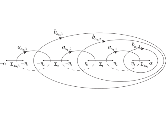
Figure 9: The Riemann surface $\mathcal{S}_{\alpha_{2}}$ of genus three and its basis $\{{a}_{\alpha_{2},j},{b}_{\alpha_{2},j}\}~{}(j=1,2,3)$ of circles.

The normalized holomorphic differentials associated with the Riemann surface $\mathcal{S}_{\alpha_{2}}$ are denoted as $\omega_{\alpha_{2},j}~{}(j=1,2,3)$. Suppose the period matrix of $\omega_{\alpha_{2},j}$ is $\tau_{\alpha_{2}}:=(\tau_{\alpha_{2},ij})_{3\times 3}$ with the symmetry $\tau_{\alpha_{2},11}=\tau_{\alpha_{2},33},\tau_{\alpha_{2},12}=\tau_{\alpha_{2},23}$ like the case in (3.2.2). Similarly, define the Jacobi map $J_{\alpha_{2}}(\lambda)$ as

$$J_{\alpha_{2}}(\lambda)=\int_{\alpha_{2}}^{\lambda}\hat{\omega}_{\alpha_{2}}:=\int_{\alpha_{2}}^{\lambda}\begin{pmatrix}\omega_{\alpha_{2},1}+\omega_{\alpha_{2},3}\\ 2\omega_{\alpha_{2},2}\end{pmatrix},$$ (4.3.15)

and the corresponding period matrix is

$$\hat{\tau}_{\alpha_{2}}=\begin{pmatrix}\tau_{\alpha_{2},11}+\tau_{\alpha_{2},31}&\tau_{\alpha_{2},12}+\tau_{\alpha_{2},32}\\ 2\tau_{\alpha_{2},21}&2\tau_{\alpha_{2},22}\end{pmatrix}.$$ (4.3.16)

In fact, the Jacobi map $J_{\alpha_{2}}(\lambda)$ satisfies the similar properties in (3.2.6) and (3.2.7) just by replacing $\eta_{4}$ with $\alpha_{2}$. In addition, by the symmetry of $J_{\alpha_{2}}(\lambda)$ like that in (3.2.8), it is derived that $d_{\alpha_{2}}=d=\frac{e_{2}+e_{1}}{2}$. According to the second and third jump conditions in (4.3.2), it follows

$${\Omega}_{\alpha_{2},1}=24\int_{\alpha_{2}}^{\eta_{3}}\frac{Q_{\alpha_{2},2}(\zeta)}{R_{\alpha_{2}}(\zeta)}d\zeta-8\xi\int_{\alpha_{2}}^{\eta_{3}}\frac{Q_{\alpha_{2},1}(\zeta)}{R_{\alpha_{2}}(\zeta)}d\zeta,$$ (4.3.17)

$${\Omega}_{\alpha_{2},0}={\Omega}_{\alpha_{2},1}+24\int_{\eta_{2}}^{\eta_{1}}\frac{Q_{\alpha_{2},2}(\zeta)}{R_{\alpha_{2}}(\zeta)}d\zeta-8\xi\int_{\eta_{2}}^{\eta_{1}}\frac{Q_{\alpha_{2},1}(\zeta)}{R_{\alpha_{2}}(\zeta)}d\zeta.$$

Moreover, since the reconstruction formula involves the derivative with respect to $x$, the following lemma is necessary.

Lemma 4.7.

The following identities are established

$$\partial_{x}(tg^{\prime}_{\alpha_{2}}(\lambda))=1-\frac{Q_{\alpha_{2},1}(\lambda)}{R_{\alpha_{2}}(\lambda)},\ \partial_{x}\left(t\Omega_{\alpha_{2},1}\right)=\oint_{b_{1}}\frac{Q_{\alpha_{2},1}(\zeta)}{R_{\alpha_{2}}(\zeta)}d\zeta,\ \partial_{x}\left(t\Omega_{\alpha_{2},0}\right)=\oint_{b_{2}}\frac{Q_{\alpha_{2},1}(\zeta)}{R_{\alpha_{2}}(\zeta)}d\zeta.$$ (4.3.18)

Proof.

From the definition of the function $g^{\prime}_{\alpha_{2}}(\lambda)$ in (4.3.4), it is seen that

$$\partial_{x}(tg^{\prime}_{\alpha_{2}}(\lambda))=1-\frac{Q_{\alpha_{2},1}(\lambda)}{R_{\alpha_{2}}(\lambda)}+\partial_{\alpha_{2}}\left(12t\frac{Q_{\alpha_{2},2}(\lambda)}{R_{\alpha_{2}}(\lambda)}-x\frac{Q_{\alpha_{2},1}(\lambda)}{R_{\alpha_{2}}(\lambda)}\right)\partial_{x}{\alpha_{2}},$$

and since $\partial_{\alpha_{2}}\left(12t\frac{Q_{\alpha_{2},2}(\lambda)}{R_{\alpha_{2}}(\lambda)}d\lambda-x\frac{Q_{\alpha_{2},1}(\lambda)}{R_{\alpha_{2}}(\lambda)}d\lambda\right)$ doesn’t have singularities at $\pm\alpha_{2}$ and $\infty$, the term $12t\frac{Q_{\alpha_{2},2}(\lambda)}{R_{\alpha_{2}}(\lambda)}d\lambda-x\frac{Q_{\alpha_{2},1}(\lambda)}{R_{\alpha_{2}}(\lambda)}d\lambda$ is a holomorphic differential 1-form. Simultaneously, it is normalized to zero on the $a_{\alpha_{2},j}~{}(j=1,2,3)$-cycles, thus by Riemann bilinear relation one has

$$\partial_{\alpha_{2}}\left(12t\frac{Q_{\alpha_{2},2}(\lambda)}{R_{\alpha_{2}}(\lambda)}-x\frac{Q_{\alpha_{2},1}(\lambda)}{R_{\alpha_{2}}(\lambda)}\right)=0.$$

On the other hand, it is obvious that

$$\Omega_{\alpha_{2},1}=-\oint_{b_{1}}(g^{\prime}(\zeta)+12\zeta^{2}-4\xi)d\zeta,\ \Omega_{\alpha_{2},0}=-\oint_{b_{2}}(g^{\prime}(\zeta)+12\zeta^{2}-4\xi)d\zeta.$$

So it follows that

$$\partial_{x}\left(t\Omega_{\alpha_{2},1}\right)=-\partial_{x}\left(t\oint_{b_{1}}(g^{\prime}(\zeta)+12\zeta^{2}-4\xi)d\zeta\right)=\oint_{b_{1}}\frac{Q_{\alpha_{2},1}(\zeta)}{R_{\alpha_{2}}(\zeta)}d\zeta,$$

$$\partial_{x}\left(t\Omega_{\alpha_{2},0}\right)=-\partial_{x}\left(t\oint_{b_{2}}(g^{\prime}(\zeta)+12\zeta^{2}-4\xi)d\zeta\right)=\oint_{b_{2}}\frac{Q_{\alpha_{2},1}(\zeta)}{R_{\alpha_{2}}(\zeta)}d\zeta.$$

 

Thus for $\xi_{crit}^{(2)}<\xi<\xi_{crit}^{(3)}$, the following theorem holds.

Theorem 4.8.

For $\xi=\frac{x}{4t}$, in the region $\xi_{crit}^{(2)}<\xi<\xi_{crit}^{(3)}$, the large-time asymptotic behavior of the solution to the KdV equation with two-genus soliton gas potential is described by

$$u(x,t)=-\left(2b_{\alpha_{2},1}+{\sum_{j=1}^{3}\eta_{j}^{2}+\alpha_{2}^{2}}+2\partial_{x}^{2}\log\left(\Theta\left(\frac{\Omega_{\alpha_{2}}}{2\pi i};\hat{\tau}_{\alpha_{2}}\right)\right)\right)+\mathcal{O}\left(\frac{1}{t}\right),$$ (4.3.19)

where the parameter $\alpha_{2}$ is determined by (4.3.7).

Proof.

Recall that

$$Y_{1}(\lambda)=\left(S_{\alpha_{2},1}^{\infty}(\lambda)+\frac{(\mathcal{E}_{\alpha_{2},1}(x,t))_{1}}{t\lambda}+\mathcal{O}\left(\frac{1}{\lambda^{2}}\right)\right)e^{-tg_{\alpha_{2}}(\lambda)}f_{\alpha_{2}}(\lambda)^{-1},$$

in which the function $f_{\alpha_{2}}(\lambda)$ behaves

$$f_{\alpha_{2}}(\lambda)=1+\frac{f_{\alpha_{2}}^{(1)}(\alpha_{2})}{\lambda}+\mathcal{O}\left(\frac{1}{\lambda^{2}}\right),$$

with

$$f_{\alpha_{2}}^{(1)}(\alpha_{2})=\left(\int_{\eta_{1}}^{\eta_{2}}+\int_{\eta_{3}}^{\alpha_{2}}\right)\frac{\zeta^{4}\log{r(\zeta)}}{R_{\alpha_{2}}(\zeta)}\frac{d\zeta}{\pi i}+\Delta_{\alpha_{2},0}\int_{-\eta_{1}}^{\eta_{1}}\frac{\zeta^{4}}{R_{\alpha_{2}}(\zeta)}\frac{d\zeta}{2\pi i}+\Delta_{\alpha_{2},1}\int_{\eta_{2}}^{\eta_{3}}\frac{\zeta^{4}}{R(\zeta)}\frac{d\zeta}{\pi i},$$

and the term $\frac{(\mathcal{E}_{\alpha_{2},1}(x,t))_{1}}{t\lambda}$ is first entry of the error vector subject to the modulated two-phase wave region. Similar to the modulated one-phase case, one can conclude that the local parametrix near $\pm\alpha_{2}$ and $\pm\eta_{j}$ ($j=1,2,3$) can be described by Airy function and modified Bessel function respectively and both of them contribute the error term $\mathcal{O}(t^{-1})$ in the asymptotic behavior of potential $u(x,t)$ for $t\to+\infty$.

The derivative of the term $e^{-tg_{\alpha_{2}}(\lambda)}$ has the asymptotics

$$\partial_{x}e^{-tg_{\alpha_{1}}(\lambda)}=-\frac{1}{\lambda}\left[\frac{\eta_{1}^{2}+\eta_{2}^{2}+\eta_{3}^{2}+\alpha_{2}^{2}}{2}+b_{\alpha_{2},1}\right]+\mathcal{O}\left(\frac{1}{\lambda^{2}}\right).$$

In addition, from Lemma 4.7, it follows from Reciprocity theorem [4] that

$$\sum\mathrm{res}_{\infty_{\pm}}\frac{\omega_{\alpha_{2},1}}{\lambda}=\frac{\partial_{x}\left(t\Omega_{\alpha_{2},1}\right)}{2\pi i},\ \sum\mathrm{res}_{\infty_{\pm}}\frac{\omega_{\alpha_{2},2}}{\lambda}=\frac{\partial_{x}(t\Omega_{\alpha_{2},0})}{2\pi i},\ \sum\mathrm{res}_{\infty_{\pm}}\frac{\omega_{\alpha_{2},3}}{\lambda}=\frac{\partial_{x}(t\Omega_{\alpha_{2},1})}{2\pi i}.$$

Recalling $J_{\alpha_{2}}(\infty)=(e_{1}+e_{2})/2$, the Jacobi map $J_{\alpha_{2}}(\lambda)$ has the asymptotics

$$J_{\alpha_{2}}(\lambda)=\frac{e_{1}+e_{2}}{2}-\frac{\begin{pmatrix}\partial_{x}(t\Omega_{\alpha_{2},1})&\partial_{x}(t\Omega_{\alpha_{2},0})\end{pmatrix}^{T}}{\lambda}+\mathcal{O}\left(\frac{1}{\lambda^{2}}\right),\quad\lambda\to\infty.$$

Since $\partial_{x}{\Delta_{\alpha_{2}}}=\mathcal{O}\left(\frac{1}{t}\right)$ as $t\to+\infty$, the Jacobi map $J_{\alpha_{2}}(\lambda)$ can be rewritten as

$$J_{\alpha_{2}}(\lambda)=\frac{e_{1}+e_{2}}{2}-\frac{\partial_{x}(\Omega_{\alpha_{2}})}{\lambda}+\mathcal{O}\left(\frac{1}{\lambda^{2}}\right)+\mathcal{O}\left(\frac{1}{t}\right).$$

Thus the expansion of the function $S_{\alpha_{2},1}^{\infty}(\lambda)$ as $\lambda\to\infty$ is expressed by

$${S}^{\infty}_{\alpha_{2},1}(\lambda) =1-\frac{1}{\lambda}\left[\nabla\log\left(\Theta\left(\frac{\Omega_{\alpha_{2}}}{2\pi i};\hat{\tau}_{\alpha_{2}}\right)\right)-\nabla\log(\Theta(0;\hat{\tau}_{\alpha_{2}}))\right]\cdot\frac{\partial_{x}(\Omega_{\alpha_{2}})}{2\pi i}+\mathcal{O}\left(\frac{1}{t}\right)+\mathcal{O}\left(\frac{1}{\lambda^{2}}\right),$$

$$=1-\frac{1}{\lambda}\partial_{x}\log\left(\Theta\left(\frac{\Omega_{\alpha_{2}}}{2\pi i};\hat{\tau}_{\alpha_{2}}\right)\right)+\mathcal{O}\left(\frac{1}{t}\right)+\mathcal{O}\left(\frac{1}{\lambda^{2}}\right).$$

Therefore, the asymptotics $\partial_{x}f_{\alpha_{2}}^{(1)}=\mathcal{O}\left(\frac{1}{t}\right)$ for $t\to+\infty$ and all the formulae above result in the large-time asymptotic behavior of $u(x,t)$ as

$$u(x,t)=-\left(2b_{\alpha_{2},1}+{\sum_{j=1}^{3}\eta_{j}^{2}+\alpha_{2}^{2}}+2\partial_{x}^{2}\log\left(\Theta\left(\frac{\Omega_{\alpha_{2}}}{2\pi i};\hat{\tau}_{\alpha_{2}}\right)\right)\right)+\mathcal{O}\left(\frac{1}{t}\right),\quad t\to+\infty.$$

 

4.4 Unmodulated two-phase wave region

For $\xi>\xi_{crit}^{(3)}$, the large-time behavior of $u(x,t)$ is described by an unmodulated two-phase Riemann-Theta function. Similar to the case in Section 4.2.1, we only need to modify relevant notations, such as $g_{\alpha_{2}}$, $R_{\alpha_{2}}(\lambda)$, $\mathcal{S}_{\alpha_{2}}$, $\Omega_{\alpha_{2}}$, and $\Delta_{\alpha_{2}}$ in Section 4.3 by replacing $\alpha_{2}$ with $\eta_{4}$. Similarly, one can verify that $g_{\eta_{4}}$ and $f_{\eta_{4}}$ can still deform the RH problem for $Y(x,t;\lambda)$ into a model problem $S_{\eta_{4}}^{\infty}(\lambda)$. Indeed, the model problem $S_{\eta_{4}}^{\infty}(\lambda)$ is also similar to $S^{\infty}(\lambda)$ in (3.0.11) with the same jump contours, but the diagonal matrices are replaced by $e^{(t{\Omega}_{j,\eta_{4}}+{\Delta}_{j,\eta_{4}})\sigma_{3}}$ for $j=0,1$. We omit all the details here for brevity. Thus for $\xi>\xi_{crit}^{(3)}$, the following theorem holds.

Theorem 4.9.

For $\xi=\frac{x}{4t}$, in the region $\xi_{crit}^{(3)}<\xi$, the large-time asymptotic behavior of the solution to the KdV equation with two-genus soliton gas potential is described by

$$u(x,t)=-\left(2b_{\eta_{4},1}+{\sum_{j=1}^{4}\eta_{j}^{2}}+2\partial_{x}^{2}\log\left(\Theta\left(\frac{\Omega_{\eta_{4}}}{2\pi i};\hat{\tau}_{\eta_{4}}\right)\right)\right)+\mathcal{O}\left(\frac{1}{t}\right),$$ (4.4.1)

where $\hat{\tau}_{\eta_{4}}=\hat{\tau}$ in (3.2.4) and $b_{\eta_{4}},\Omega_{\eta_{4}}=\begin{pmatrix}{t\Omega_{\eta_{4},1}+{\Delta_{\eta_{4},1}}}&{t\Omega_{\eta_{4},0}+{\Delta_{\eta_{4},0}}}\end{pmatrix}^{T}$ are defined by (4.3.6) and (4.3.17), respectively.

Remark 4.10.

The error estimation is quite similar with the discussion in Section 3 and the parametrix near $\pm\eta_{j}$ ($j=1,2,3,4$) can be described by the modified Bessel functions [21], which contribute the $\mathcal{O}(t^{-1})$ term in (4.4.1).

5 The $\mathcal{N}$-genus KdV soliton gas

Figure 10: The long-time asymptotic regions of the $\mathcal{N}$-genus KdV soliton gas potential in the $x$-$t$ half plane.

In general, when constructing the RH problem for the KdV equation, one can consider the discrete spectral points gathering in $2\mathcal{N}$ symmetric bands, where the integer $\mathcal{N}>2$. These bands are defined as $\Sigma_{2j-1}:=(i\eta_{j},i\eta_{j+1})$ and $\Sigma_{2j}:=(-i\eta_{j+1},-i\eta_{j})$, for $j=1,2,\cdots,\mathcal{N}$. Consequently, the RH problem for the $\mathcal{N}$-genus KdV soliton gas is given by:

$$X_{+}^{(\mathcal{N})}(\lambda)=X_{-}^{(\mathcal{N})}(\lambda)\begin{cases}\begin{aligned} &\begin{pmatrix}1&-2ir_{2}(\lambda)e^{-2i\lambda x}\\ 0&1\end{pmatrix},&&\lambda\in i\Sigma_{1,3,\ldots,2j-1},\\ &\begin{pmatrix}1&\\ 2ir_{2}(\lambda)e^{2i\lambda x}&1\end{pmatrix},&&\lambda\in i\Sigma_{2,4,\ldots,2j},\end{aligned}\end{cases}$$ (5.0.1)

$$X^{(\mathcal{N})}(\lambda)\to\begin{pmatrix}1&1\end{pmatrix},\quad\lambda\to\infty,$$ (5.0.2)

$$X^{(\mathcal{N})}(-\lambda)=X^{(\mathcal{N})}(\lambda)\begin{pmatrix}0&1\\ 1&0\end{pmatrix}.$$ (5.0.3)

Similarly, the $\mathcal{N}$-genus KdV soliton gas potential can be constructed by

$$u(x)=2\frac{\mathrm{d}}{\mathrm{d}x}\left(\lim_{\lambda\rightarrow\infty}\frac{\lambda}{i}\left(X_{1}^{(\mathcal{N})}(\lambda)-1\right)\right),$$ (5.0.4)

where $X_{1}^{(\mathcal{N})}(\lambda)$ is the first component of $X^{(\mathcal{N})}(\lambda)$.

Following the similar procedure outlined in Section 3, the large $x$ behavior of the $\mathcal{N}$-genus KdV soliton gas potential is described by:

$$u_{\mathcal{N}}(x)=\begin{cases}\begin{aligned} &-\left(2\alpha_{\mathcal{N}}+\sum_{j=1}^{2\mathcal{N}}\eta_{j}^{2}+2\partial_{x}^{2}\log\left(\tilde{\Theta}\left(\frac{\Omega_{\mathcal{N}}}{2\pi i};\tau_{\mathcal{N}}\right)\right)\right)+\mathcal{O}\left(\frac{1}{x}\right),&&x\to+\infty,\\ &\mathcal{O}(e^{-c|x|}),&&x\to-\infty,\end{aligned}\end{cases}$$ (5.0.5)

where $\alpha_{\mathcal{N}}$ is a parameter and $\tilde{\Theta}(\bullet;\tau_{\mathcal{N}})$ is the $\mathcal{N}$-phase Riemann-Theta function with period matrix $\tau_{\mathcal{N}}$ and $\mathcal{N}$-dimensional column vector $\Omega_{\mathcal{N}}$.

As the $\mathcal{N}$-genus soliton gas potential (5.0.4) evolves according to the KdV equation (1.0.1) for $t\to\infty$, the long-time asymptotic regions can be classified into $2\mathcal{N}+1$ regions in the $x$-$t$ plane, which from left to right are rapid decay, modulated one-phase wave, unmodulated one-phase wave, $\cdots$, modulated $\mathcal{N}$-phase wave and unmodulated $\mathcal{N}$-phase wave, respectively (see Fig. 10 for detail).

References

• [1] M. J. Ablowitz, P. A. Clarkson, Solitons, nonlinear evolution equations and inverse scattering, Cambridge University Press, 1991.
• [2] M. J. Ablowitz, J. T. Cole, G. A. El, M. A. Hoefer, X.-D. Luo, Soliton–mean field interaction in Korteweg–de Vries dispersive hydrodynamics, Stud. Appl. Math., 151 (2023), pp. 795–856.
• [3] M. Bertola, R. Jenkins, A. Tovbis, Partial degeneration of finite gap solutions to the Korteweg-de Vries equation: soliton gas and scattering on elliptic backgrounds, Nonlinearity, 36 (2023), pp. 3622–3660.
• [4] M. Bertola, Tau functions in integrable systems: theory and applications, 2018. (available at: http://mypage.concordia.ca/mathstat/bertola/ThetaCourse/ThetaCourse.pdf)
• [5] M. Bertola, T. Grava, G. Orsatti, Soliton Shielding of the Focusing Nonlinear Schrödinger Equation, Phys. Rev. Lett., 130 (2023), 127201.
• [6] M. Bertola, T. Grava, G. Orsatti, $\bar{\partial}$-problem for focusing nonlinear Schrödinger equation and soliton shielding, arXiv:2409.14825.
• [7] D. Bilman, T. Trogdon, On numerical inverse scattering for the Korteweg-de Vries equation with discontinuous step-like data, Nonlinearity, 33 (2020), pp. 2211-2269.
• [8] T. Claeys, T. Grava, Solitonic asymptotics for the Korteweg-de Vries equation in the small dispersion limit, SIAM J. Math. Anal., 42 (2010), pp.2132-2154.
• [9] G. Biondini, G. A. El, X.-D. Luo, J. Oregero, A. Tovbis, Breather gas fission from elliptic potentials in self-focusing media, arXiv:2407.15758.
• [10] C. Charlier, J. Lenells, Miura transformation for the “good” Boussinesq equation, Stud. Appl. Math., 152 (2024), pp. 73–110.
• [11] T. Bonnemain, B. Doyon, G. A. El, Generalized hydrodynamics of the KdV soliton gas, J. Phys. A, 55 (2022), 374004.
• [12] P. Deift, X. Zhou, A Steepest descent method for oscillatory Riemann-Hilbert problems. Asymptotics for the mKdV equation, Ann. Math., 137 (1993), pp. 295-368.
• [13] P. Deift, S. Venakides, X. Zhou, The collisionless shock region for the long-time behavior of solutions of the KdV equation, Comm. Pure Appl. Math., 46 (1994), pp. 199-206.
• [14] P. Deift, S. Venakides, X. Zhou, New results in small dispersion KdV by an extension of the steepest descent method for Riemann-Hilbert problems, Int. Math. Res. Not., 6 (1997), pp. 285-299.
• [15] S. Dyachenko, D. Zakharov, V. Zakharov, Primitive potentials and bounded solutions of the KdV equation, Phys. D, 333 (2016), pp. 148-156.
• [16] I. Egorova, Z. Gladka, V. Kotlyarov, G. Teschl, Long-time asymptotics for the Korteweg-de Vries equation with step-like initial data, Nonlinearity, 26 (2013), pp. 1839-1864.
• [17] G. A. El, The thermodynamic limit of the Whitham equations, Phys. Lett. A, 311 (2003), pp. 374-383.
• [18] G. A. El, A. M. Kamchatnov, M. V. Pavlov, S. A. Zykov, Kinetic equation for a soliton gas and its hydrodynamic reductions, J. Nonlinear Sci., 21 (2011), pp. 151-191.
• [19] E. V. Ferapontov, M. V. Pavlov, Kinetic equation for soliton gas: integrable reductions, J. Nonlinear Sci., 32 (2022), 26.
• [20] M. Girotti, T. Grava, R. Jenkins, K. D. T.-R. McLaughlin, Rigorous asymptotics of a KdV soliton gas, Comm. Math. Phys., 384 (2021), pp. 733-784.
• [21] M. Girotti, T. Grava, R. Jenkins, K. D. T.-R. McLaughlin, A. Minakov, Soliton versus the gas: Fredholm determinants, analysis, and the rapid oscillations behind the kinetic equation, Comm. Pure Appl. Math., 76 (2023), pp. 3233-3299.
• [22] T. Grava, Whitham modulation equations and application to small dispersion asymptotics and long time asymptotics of nonlinear dispersive equations, In: M. Onorato, S. Resitori, F. Baronio (eds), Rogue and Shock Waves in Nonlinear Dispersive Media, Lect. Notes Phys., vol. 926, Springer, 2016.
• [23] R. Gong, D. S. Wang, Modulation theory of soliton-mean flow in KdV equation with box type initial data, Preprint, arXiv:2405.20826, 2024.
• [24] P. D. Lax, Integrals of nonlinear equations of evolution and solitary waves, Comm. Pure Appl. Math., 21 (1968), pp. 467-490.
• [25] C. D. Levermore, The hyperbolic nature of the zero dispersion KdV limit, Comm. Partial Differential Equations, 13(4) (1988), pp. 495-514.
• [26] K. D. T.-R. McLaughlin, P. V. Nabelek, A Riemann-Hilbert problem approach to infinite gap Hill’s operators and the Korteweg–de Vries equation, Int. Math. Res. Not., 2 (2021), pp. 1288-1352.
• [27] P. D. Miller, S. R. Clarke, An exactly solvable model for the interaction of linear waves with Korteweg-de Vries solitons, SIAM J. Math. Anal., 33 (2001), pp.261-285.
• [28] I. Egorova, Z. Gladka, V. Kotlyarov, G. Teschl, Long-time asymptotics for the Korteweg-de Vries equation with step-like initial data, Nonlinearity, 26 (2013), pp. 1839-1864.
• [29] A. Tovbis, F. Wang, Recent developments in spectral theory of the focusing NLS soliton and breather gases: the thermodynamic limit of average densities, fluxes and certain meromorphic differentials; periodic gases, J. Phys. A, 55 (2022), 424006
• [30] M. Piorkowski, G. Teschl, A scalar Riemann–Hilbert problem on the torus: applications to the KdV equation, Anal. Math. Phys., 12, (2022) 112.
• [31] E. G. Shurgalina, E. N. Pelinovsky, Nonlinear dynamics of a soliton gas: Modified Korteweg–de Vries equation framework, Phys. Lett. A, 380 (2016), pp. 2049-2053.
• [32] P. Zhao, E. Fan, A Riemann-Hilbert method to algebro-geometric solutions of the Korteweg–de Vries equation, Phys. D, 454 (2023), 133879.
• [33] V. Zakharov, Kinetic equation for solitons, Sov. Phys. JETP, 33(3) (1971), pp. 538-541.