Thermal effects on warm chromoinflation

Abstract

We explore a model of a pseudo-Nambu-Goldstone boson inflaton field coupled to a non-Abelian $SU(2)$ gauge field. This model naturally leads to a warm inflation scenario, where the inflationary dynamics is dominated by thermal dissipation. In this work, we consider a scenario where the inflaton, an axion-like field, is coupled to the $SU(2)$ gauge field, similar to chromoinflation models. Both the inflaton and the gauge field with a non-vanishing vacuum expectation value are coupled to a thermal radiation bath. We demonstrate that the presence of the thermal bath during warm chromoinflation induces a thermal plasma mass for the background gauge field. This thermal mass can significantly disrupt the dynamics of the background gauge field, thereby driving it to its trivial null solution.

I Introduction

Warm inflation (WI) Berera:1995wh ; Berera:1995ie ; Berera:1998px has recently seen successful implementations in models featuring pseudo-Nambu-Goldstone scalar fields Bastero-Gil:2016qru ; Bastero-Gil:2019gao ; Berghaus:2019whh ; Laine:2021ego ; DeRocco:2021rzv . These models often involve axion-like fields directly coupled to non-Abelian gauge fields. The dissipation of the axion-inflaton into gauge fields can naturally lead to a thermal radiation bath, even from initial vacuum conditions Laine:2021ego ; DeRocco:2021rzv . This thermal bath is a hallmark of the warm inflationary regime.

The explicit realization of consistent warm inflation dynamics in these models is a significant achievement. WI has emerged as a promising inflation model that aligns with effective field theory and potentially finds a ultraviolet (UV) completion in quantum gravity Das:2018rpg ; Motaharfar:2018zyb ; Goswami:2019ehb ; Berera:2019zdd ; Kamali:2019xnt ; Berera:2020iyn ; Das:2020xmh ; Brandenberger:2020oav ; Motaharfar:2021egj . Therefore, constructing explicit models of warm inflation and exploring their implications has become increasingly important.

In this work, we investigate an axion warm inflation (WI) model incorporating a Chern-Simons interaction between the axion inflaton field and a $SU(2)$ gauge field. It is well-established Maleknejad:2011jw ; Maleknejad:2016qjz ; Adshead:2012kp ; Kamali:2019ppi that, in addition to the background inflaton field, an isotropic solution for the $SU(2)$ gauge field is also permissible (for a review, see, e.g. Ref. Maleknejad:2012fw ). This background gauge field can substantially influence the evolutionary dynamics of the expanding system at both the background and perturbation levels.

Here, we demonstrate that the presence of a thermal bath naturally induces a plasma mass for the background gauge field. This thermal mass contribution to the gauge background field, similar to the thermal mass affecting the inflaton equation in warm inflation Berera:1998gx ; Yokoyama:1998ju , can potentially disrupt the slow-roll conditions for the gauge field, driving it towards a vanishing value. We investigate the impact of these thermal effects on the background dynamics and illustrate our results using a commonly employed axion potential.

This paper is organized as follows. In Sec. II, we briefly review the background dynamics of chromoinflation in the context of warm inflation. In Sec. III, we compute the leading order thermal contributions to the background dynamics. In Sec. IV, we illustrate our results by explicitly studying the dynamics in a case of axion-like potential. In Sec. V, we give our concluding remarks.

Throughout this paper, we work with the natural units, in which the speed of light, Planck’s constant and Boltzmann’s constant are all set to $1$, $c=\hbar=k_{B}=1$. We work in the context of a spatially flat homogeneous and isotropic background metric with scale factor $a(t)$, where $t$ is physical time. We also work with the reduced Planck mass, defined as $M_{\rm Pl}=(8\pi G)^{-\frac{1}{2}}\simeq 2.44\times 10^{18}$ GeV and where $G$ is Newton’s gravitational constant. The Hubble expansion rate is $H(t)={\dot{a}(t)}/a(t)$, where an overdot denotes the derivative with respect to time.

II The Axion Warm Inflation Model

We work with a minimal setting for an axion-like field $\phi$ making the role of the inflaton and coupled to a non-Abelian $SU(2)$ gauge field $A_{\mu}$ with the standard dimension five interaction, with action in a FLRW metric,

$$S = \int d^{4}xa^{3}(t)\left[\frac{1}{2}(\partial_{\mu}\phi)^{2}-V(\phi)-\frac{1}{4}F_{\mu\nu}^{c}F^{c\,\mu\nu}\right.$$ (1)

$$- \left.\frac{\lambda}{4f}\phi F_{\mu\nu}^{c}\tilde{F}^{c\,\mu\nu}\right],$$

where $c=1,\ldots,N_{c}^{2}-1$ is the group index, with $N_{c}=2$ for $SU(2)$, $f$ is the axion decay constant, $F_{\mu\nu}^{a}=\partial_{\mu}A_{\nu}^{a}-\partial_{\nu}A_{\mu}^{a}+g\epsilon^{abc}A_{\mu}^{b}A_{\nu}^{c}$ is the gauge field tensor, $\tilde{F}^{c\,\mu\nu}$ is its dual,

$$\tilde{F}^{c\,\mu\nu}=\frac{\epsilon^{\mu\nu\rho\sigma}}{2a^{3}(t)}F_{\rho\sigma}^{c},$$ (2)

and $a(t)$ is the scale factor.

The $SU(2)$ gauge field admit a homogeneous vacuum expectation value (VEV), defined as Maleknejad:2011jw ; Maleknejad:2016qjz ; Adshead:2012kp

$$\bar{A}^{c}_{i}=a(t)\psi(t)\delta^{c}_{i},\;\;\;\;\bar{A}^{c}_{0}=0,$$ (3)

which leads to the gauge field strength components,

$$\bar{F}^{c\,0i}=-\bar{F}^{c,i0}=-\frac{1}{a}(H\psi+\dot{\psi})\delta^{ci},\;\;\;\bar{F}^{c\,ij}=\frac{g}{a^{2}}\psi^{2}\epsilon^{cij},$$

$$\bar{F}_{0i}^{c}=-\bar{F}_{i0}^{c}=a(H\psi+\dot{\psi})\delta_{i}^{c},\;\;\;\bar{F}_{ij}^{c}=ga^{2}\psi^{2}\epsilon_{ij}^{c}.$$ (4)

Note that in chromoinflation Maleknejad:2011jw ; Maleknejad:2016qjz ; Adshead:2012kp the coupling $\lambda$ between the inflaton $\phi$ and the gauge fields in the interaction term in Eq. (1) is assumed to be an independent constant. Typically, a consistent background evolution for the inflaton and gauge field is achieved for large couplings, or more generally, $\lambda M_{\rm Pl}/f\gg 1$. How to achieve such large couplings in effective theories has been discussed recently for example in Refs. Agrawal:2018mkd ; Holland:2020jdh . Note that in the axion dynamics case, the coupling $\lambda$ is simply related to the gauge coupling $g$ by $\lambda=g^{2}/(8\pi^{2})$.

The inflaton (axion) field has been shown to dissipate into radiation bath gauge fields, which forms a thermal bath with temperature $T$ and whose dissipation coefficient is given by Berghaus:2019whh ; Laine:2021ego

$$\Upsilon(T)=\kappa\frac{T^{3}}{f^{2}},$$ (5)

where $\kappa$ is given by

$$\kappa\simeq 1.2\pi\frac{g^{4}(g^{2}N_{c})^{3}(N_{c}^{2}-1)}{(64\pi^{3})^{2}}\left[\ln\left(\frac{m_{D}}{\gamma}\right)+3.041\right],$$ (6)

where $m_{D}^{2}=g^{2}N_{c}T^{2}/3$ is the Debye mass squared of the Yang-Mills plasma and $\gamma$ is given by the solution of Moore:2010jd

$$\gamma=\frac{g^{2}N_{c}T}{4\pi}\left[\ln\left(\frac{m_{D}}{\gamma}\right)+3.041\right].$$ (7)

Explicitly, this gives for $\kappa$ the result

$$\kappa = 0.3\alpha^{5}N_{c}^{3}(N_{c}^{2}-1)W\left(e^{3.041}\sqrt{\frac{4\pi}{3\alpha N_{c}}}\right),$$ (8)

where $\alpha=g^{2}/(4\pi)$ is the fine structure Yang-Mills coupling and $W(x)$ is the Lambert function, given by the principal solution of $x=we^{w}$. For $N_{c}=2$ and assuming e.g. $\alpha=0.1$, we obtain that $\kappa\simeq 2.4\times 10^{-4}$.

II.1 Background Evolution

Implementations of warm inflation in the context of chromoinflation have been considered in some recent works Yeasmin:2022ncm ; Mukuno:2024yoa . At the background level, the energy density related to the inflaton field $\phi$, the VEV $\psi$ of the Yang-Mills gauge field and the thermal bath are, respectively, given by

$$\rho_{\phi}=\frac{1}{2}\dot{\phi}^{2}+V(\phi),$$ (9)

$$\rho_{YM}=\frac{3}{2}\left(\dot{\psi}+H\psi\right)^{2}+\frac{3}{2}g^{2}\psi^{4},$$ (10)

$$\rho_{r}=C_{r}T^{4},$$ (11)

where $C_{r}=g_{*}\pi^{2}/30$ and $g_{*}$ denotes the radiation bath degrees of freedom. In the present work we assume that the radiation bath is constituted primarily by the gauge field fluctuations, which then gives $g_{*}=2(N_{c}^{2}-1)=6$ for the case of the (massless) $SU(2)$ Yang-Mills fields.

Likewise, the evolution equations for the inflaton field $\phi$, the Yang-Mills VEV $\psi$ and the radiation energy density $\rho_{r}$ are given by

$$\!\!\!\!\!\!\!\!\!\!\!\!\!\!\!\ddot{\phi}+3H\dot{\phi}+V_{,\phi}+3\frac{\lambda}{f}g\psi^{2}(\dot{\psi}+H\psi)+\Upsilon\dot{\phi}=0,$$ (12)

$$\!\!\!\!\!\!\!\!\!\!\!\!\!\!\!\ddot{\psi}+3H\dot{\psi}+(2H^{2}+\dot{H})\psi+2g^{2}\psi^{3}-\frac{\lambda g}{f}\psi^{2}\dot{\phi}=0,$$ (13)

$$\!\!\!\!\!\!\!\!\!\!\!\!\!\!\!\dot{\rho}_{r}+4H\rho_{r}=\Upsilon\dot{\phi}^{2},$$ (14)

where the dissipation coefficient $\Upsilon$ is given by Eq. (5).

The slow-roll variables can be defined as Maleknejad:2016qjz

$$\epsilon_{\psi}=\frac{\dot{\psi}}{H\psi}~{}~{}~{}~{}~{}~{}\eta_{\psi}=-\frac{\ddot{\psi}}{H\psi}$$ (15)

$$\epsilon_{H}=-\frac{\dot{H}}{H^{2}}~{}~{}~{}~{}~{}~{}~{}~{}\eta_{H}=-\frac{\ddot{H}}{2H\dot{H}}$$

In the slow-roll approximation, $\epsilon_{\psi}<1$, $\eta_{\psi}<1$, $\epsilon_{H}<1$ and out of the instability condition Adshead:2013nka ; Namba:2013kia ; Dimastrogiovanni:2012ew (where the gauge perturbations become tachyonic), i.e., $g^{2}\psi^{2}/(2H^{2})>1$, the evolution of $\psi$ in Eq. (13) is simplified to

$$g\psi^{3}\simeq\frac{\lambda}{2f}\psi^{2}\dot{\phi}.$$ (16)

There are several consistency conditions that need to be satisfied such that the above equations can work properly in a warm inflation context. First, a thermal bath of particles need to be produced during inflation. This has been explicitly verified in Refs. Laine:2021ego ; DeRocco:2021rzv . Second, backreaction from the nonlinearities which are inherent of non-Abelian gauge fields need to be sufficient suppressed such that the effective theory leading to the evolution equations (12), (13) and (14) remain valid. This typically requires that we work with temperatures that remain smaller than the axion decay constant DeRocco:2021rzv , i.e., $T<f$. The warm inflation regime itself also requires $T>H$. So, we must ensure the hierarchy of energy scales: $H<T<f$. Third, to avoid the instabilities of the non-Abelian gauge field, we are required to have $g|\psi|/H>\sqrt{2}$. Forth, perturbativity also requires that the gauge coupling to be small, $\alpha<1$, such that we can also trust in the computation leading to the dissipation coefficient Eq. (5). Fifth, to ensure that there is a thermal bath of gauge particles, the temperature must remain above the confinement scale of the model Berghaus:2019whh . This implies in particular in the choice for the inflaton potential $V(\phi)$. The usual low energy infrared (IR) potential assumed for the axion cannot be used here and some ultraviolet potential need to be used. Some different potentials have been considered before, like an hybrid type of potential as used in Ref. Berghaus:2019whh . An exponential potential was considered in Ref. Das:2019acf . A simple quadratic potential for the inflaton was used in Ref. Laine:2021ego , while in Ref. DeRocco:2021rzv some axion monodromy type of potentials have been considered.

III Thermal contributions to the background dynamics

To take into account the effects of the thermal bath on the background dynamics, we will work analogously to the loop expansion in quantum field theory. This starts by expanding the fields around their vacuum background expectation values. In this work in special, we will be looking how the fluctuations around the gauge field background $\psi$ will affect the dynamics. Hence, the gauge field in (1) is expanded like $A_{\mu}\to A^{\prime}_{\mu}=\bar{A}_{\mu}(t)+A_{\mu}$, where $\langle A^{\prime}_{\mu}\rangle=\bar{A}_{\mu}(t)$, with $\bar{A}_{\mu}(t)$ given by Eq. (3) and $\langle A_{\mu}\rangle=0$. Working up to one-loop order in the fluctuations of the gauge field (i.e., second order in the gauge field fluctuations), we have for instance that

$$F^{a}_{\mu\nu}=\bar{F}_{\mu\nu}^{a}+\left(\bar{D}_{\mu}A_{\nu}\right)^{a}-\left(\bar{D}_{\nu}A_{\mu}\right)^{a}+g\epsilon^{abc}A_{\mu}^{b}A_{\nu}^{c},$$ (17)

where $\bar{F}_{\mu\nu}^{a}$ is given by Eq. (4) and

$$\bar{D}_{\mu}=\partial_{\mu}-igJ^{a}\bar{A}_{\mu}^{a},$$ (18)

is the covariant derivative expressed in terms of the background gauge field, with $J^{a}$ the generators of the $SU(2)$ group. Working in the adjunct representation of the $SU(2)$ gauge group, $(J_{a})_{bc}=\epsilon_{abc}$.

Using Eq. (17) in (1), the action, up to second order in the gauge field fluctuations, then takes the form

$$S\simeq S_{0}+\delta^{2}S,$$ (19)

where

$$S_{0} = \int d^{4}xa^{3}(t)\left[\frac{1}{2}(\partial_{\mu}\phi)^{2}-V(\phi)-\frac{1}{4}\bar{F}_{\mu\nu}^{c}\bar{F}^{c\,\mu\nu}\right.$$ (20)

$$- \left.\frac{\lambda}{4f}\phi\frac{\epsilon^{\mu\nu\rho\sigma}}{2a^{3}(t)}\bar{F}_{\mu\nu}^{c}\bar{F}_{\rho\sigma}^{c}\right]$$

$$= \int d^{4}x\,a^{3}\left[\frac{\dot{\phi}^{2}}{2}-V(\phi)+\frac{3}{2}\left(\dot{\psi}+H\psi\right)^{2}\right.$$

$$- \left.\frac{3}{2}g^{2}\psi^{4}-3\frac{\lambda}{f}g\phi\left(\dot{\psi}+H\psi\right)\psi^{2}\right],$$

is the zeroth order action in the fluctuations and $\delta^{2}S$ is the action when expanding the fields up to the second-order in the fluctuations (see also Ref. Adshead:2013nka for a similar approach for deriving the perturbation equations in chromoinflation). The Yang-Mills and Chern-Simons contributions can then be expressed as

$$\delta^{2}S_{\rm YM} = \int d^{4}x\,a^{3}\left\{-\frac{1}{2}(\bar{D}^{\mu}A^{\nu})^{a}(\bar{D}_{\mu}A_{\nu})^{a}\right.$$

$$+ \left.\frac{1}{2}(\bar{D}^{\mu}A^{\nu})^{a}(\bar{D}_{\nu}A_{\mu})^{a}-\frac{1}{2}g\epsilon^{abc}\bar{F}^{a\,\mu\nu}A_{\mu}^{b}A_{\nu}^{c}\right.$$

$$- \left.\frac{\lambda}{2f}\phi\;\frac{\epsilon^{\mu\nu\rho\sigma}}{a^{3}}\left[(\bar{D}_{\mu}A_{\nu})^{a}(\bar{D}_{\rho}A_{\sigma})^{a}\right.\right.$$

$$+ \left.\left.\frac{g}{2}\epsilon^{abc}\bar{F}^{a}_{\mu\nu}A_{\rho}^{b}A_{\sigma}^{c}\right]\right\}.$$

We still need to choose a gauge fixing term. Here, it becomes convenient to fix a gauge that depends explicitly on the background gauge field, such that (see, e.g. Srednicki:2007qs )

$$\delta^{2}S_{\rm gf}=\int d^{4}x\,a^{3}\left[-\frac{1}{2\alpha}(\bar{D}^{\mu}A^{\mu})^{a}(\bar{D}_{\nu}A_{\nu})^{a}\right],$$ (22)

and with the corresponding Faddeev-Popov ghost term,

$$\delta^{2}S_{\rm ghost}=\int d^{4}x\,a^{3}\left[(\bar{D}^{\mu}\bar{\eta})^{a}(\bar{D}_{\mu}\eta)^{a}\right],$$ (23)

where $\eta$ and $\bar{\eta}$ are the Faddeev-Popov ghost fields. Hence, by choosing the gauge $\alpha=1$ and after some manipulation of indexes in Eq. (LABEL:S2YM) and integration by parts, we obtain the result for the quadratic term in the fluctuations in the action (note that in arriving at the expression below, a term coming from the integration by parts, but not depending on the background gauge field, was neglected)

$$\delta^{2}S = \int d^{4}x\,a^{3}\left\{-\frac{1}{2}(\bar{D}^{\mu}A^{\nu})^{a}(\bar{D}_{\mu}A_{\nu})^{a}\right.$$

$$+ \left.(\bar{D}^{\mu}\bar{\eta})^{a}(\bar{D}_{\mu}\eta)^{a}-g\epsilon^{abc}\bar{F}^{a\,\mu\nu}A_{\mu}^{b}A_{\nu}^{c}\right.$$

$$- \left.\frac{\lambda}{2f}\phi\;\frac{\epsilon^{\mu\nu\rho\sigma}}{a^{3}}\left[(\bar{D}_{\mu}A_{\nu})^{a}(\bar{D}_{\rho}A_{\sigma})^{a}\right.\right.$$

$$+ \left.\left.\frac{g}{2}\epsilon^{abc}\bar{F}^{a}_{\mu\nu}A_{\rho}^{b}A_{\sigma}^{c}\right]\right\}.$$

By substituting in Eq. (LABEL:S2YM2) the equations (3) and (4), we have many terms depending on the background field $\psi$. Many of them vanishes when performing the functional integration over the fluctuations (e.g. the Chern-Simons dependent terms which are total derivatives). For the terms effectively contributing, one notices that in the presence of a nonvanishing background gauge field, both the gauge field and the ghosts acquire a mass square, $m_{A}^{2}=m_{\eta}^{2}=2g^{2}\psi^{2}$. Their functional integration lead to an effective potential for $\psi$ which can be expressed as

$$\!\!\!\!\!\Delta V_{\rm eff}(\psi) = (N_{c}^{2}-1)\int\frac{d^{4}k_{E}}{(2\pi)^{4}}\ln\left(k_{E}^{2}+2g^{2}\psi^{2}\right),$$ (25)

where $k_{E}$ refers to the (physical) momentum expressed in Euclidean spacetime. Diagrammatically, the terms contributing to the effective potential at leading order are displayed in Fig. 1.

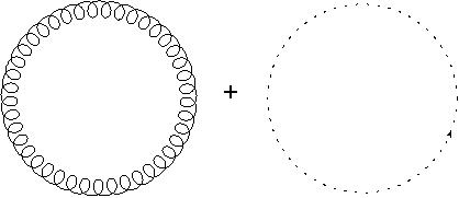
Figure 1: The vacuum diagrams contributing at leading order to the effective potential for $\psi$. The first diagram is a gauge loop diagram, with propagator with a gauge mass squared $m_{A}^{2}=2g^{2}\psi^{2}$, while the second diagram is the ghost contribution, with propagator with mass $m_{\eta}=m_{A}$.

From the usual rules of finite temperature quantum field theory Kapusta:2006pm , $k_{E}^{2}=k_{4}^{2}+{\bf k}^{2}$ and $k_{4}\equiv\omega_{n}=2\pi nT$, $n\in\mathbb{Z}$ and $\omega_{n}$ are the Matsubara’s frequencies for bosons. The integrals over momenta are expressed as

$$\int\frac{d^{4}k_{E}}{(2\pi)^{4}}\to T\sum_{k_{4}=\omega_{n}}\int\frac{d^{3}k}{\left(2\pi\right)^{3}}.$$ (26)

At zero temperature, the momentum integral in Eq. (25) is divergent. The divergent terms can be handled as usual in perturbation theory in quantum field theory by adding the appropriate renormalization counterterms in the tree-level action Eq. (20). The relevant contributions for us are the finite temperature ones, which, after performing the Matsubara’s frequency sum in Eq. (25), we are left with the thermal contribution,

$$\Delta V_{\rm eff}(\psi,T) = 2(N_{c}^{2}-1)\frac{T^{4}}{2\pi^{2}}J_{B}(y),$$ (27)

where Kapusta:2006pm

$$J_{B}(y) = \int_{0}^{\infty}dx\,x^{2}\ln\left(1-e^{-\sqrt{x^{2}+y^{2}}}\right)$$ (28)

$$\simeq -\frac{\pi^{4}}{45}+\frac{\pi^{2}}{12}y^{2}+{\cal O}(y^{3}),$$

with $y^{2}=2g^{2}\psi^{2}/T^{2}$ and the last line in Eq. (28) follows by using an expansion for $y\ll 1$. We could as well consider the additional terms in the expansion in Eq. (28). However, for our purposes of demonstrating the effects of the thermal contributions, the truncation of the series up to quadratic order for the thermal integral $J_{B}(y)$ suffices for us. We then obtain for Eq. (25) the result

$$\Delta V_{\rm eff}(\psi,T) \simeq -2(N_{c}^{2}-1)\frac{\pi^{2}}{90}T^{4}+(N_{c}^{2}-1)g^{2}\frac{T^{2}}{6}\psi^{2}.$$

The total energy density is then modified by the thermal effects, such that now we have that

$$\rho_{T} = \frac{\dot{\phi}^{2}}{2}+V(\phi)$$ (30)

$$+ \frac{3}{2}(\dot{\psi}+H\psi)^{2}+\frac{3}{2}g^{2}\psi^{4}$$

$$+ \Delta V_{\rm eff}(\psi,T)+Ts,$$

where we opted from now on to work for convenience with the entropy density $s$,

$$s = -\frac{\partial\Delta V_{\rm eff}}{\partial T}\simeq\frac{4\pi^{2}(N_{c}^{2}-1)T^{3}}{45}-\frac{(N_{c}^{2}-1)g^{2}T\psi^{2}}{3}.$$

We thus see that the presence of the thermal bath in warm chromoinflation produces not only a friction term due to the nonperturbative spharelon effects in the gauge vacua, but also leads to a thermal plasma mass for the background gauge field $\psi$,

$$m_{\psi}^{2}(T)=(N_{c}^{2}-1)\frac{g^{2}T^{2}}{3}.$$ (32)

The background field equations in warm chromoinflation then get modified such that now we have that

$$\!\!\!\!\!\!\!\!\!\!\!\!\!\!\!\ddot{\phi}+3H\dot{\phi}+V_{,\phi}+3\frac{\lambda}{f}g\psi^{2}(\dot{\psi}+H\psi)+\Upsilon\dot{\phi}=0,$$ (33)

$$\!\!\!\!\!\!\!\!\!\!\!\!\!\!\!\ddot{\psi}+3H\dot{\psi}+(2H^{2}+\dot{H})\psi+2g^{2}\psi^{3}$$

$$+m_{\psi}^{2}(T)\psi-\frac{\lambda g}{f}\psi^{2}\dot{\phi}=0,$$ (34)

$$\!\!\!\!\!\!\!\!\!\!\!\!\!\!\!T\dot{s}+3HTs=\Upsilon\dot{\phi}^{2},$$ (35)

and with the Hubble parameter given by

$$H^{2} = \frac{1}{3M_{\rm Pl}^{2}}\left[\frac{\dot{\phi}^{2}}{2}+V(\phi)+\frac{3}{2}(\dot{\psi}+H\psi)^{2}\right.$$ (36)

$$+ \left.\frac{3}{2}g^{2}\psi^{4}+\Delta V_{\rm eff}(\psi,T)+Ts\right].$$

We can qualitatively already investigate the effect of the thermal mass term in the background equation for $\psi$. In the slow-roll approximation, from Eq. (34), we obtain that

$$3H\dot{\psi}\simeq-\left[2H^{2}+m_{\psi}^{2}(T)\right]\psi-2g^{2}\psi^{3}+\frac{\lambda g}{f}\psi^{2}\dot{\phi}.$$ (37)

If we associate the right-hand side in Eq. (37) as an analogous of the field derivative of an effective potential for $\psi$ (see, e.g. Ref. Fujita:2021eue for a similar approach in cold chromoinflation), then we can define the effective potential (and assuming $\dot{\phi}$ as constant),

$$V_{\rm eff}(\psi,T)\simeq\left[2H^{2}+m_{\psi}^{2}(T)\right]\frac{\psi^{2}}{2}-\frac{\lambda g\dot{\phi}}{f}\frac{\psi^{3}}{3}+g^{2}\frac{\psi^{4}}{2}.$$ (38)

By defining the dimensionless quantities,

$$\Psi = \frac{g\psi}{H},$$

$$\xi = \frac{\lambda\dot{\phi}}{2fH},$$ (39)

$$M_{\psi} = \frac{m_{\psi}(T)}{H},$$

we are left with

$$\bar{V}_{\rm eff}(\Psi)=\left(2+M_{\psi}^{2}\right)\frac{\Psi^{2}}{2}-\frac{2\xi}{3}\Psi^{3}+\frac{\Psi^{4}}{2},$$ (40)

where $\bar{V}_{\rm eff}(\Psi)=g^{2}V_{\rm eff}(\psi,T)/H^{4}$. The potential $\bar{V}_{\rm eff}(\Psi)$ has in general three extrema: at $\Psi=0$ and at

$$\Psi_{\pm}=\frac{1}{2}\left[\xi\pm\sqrt{\xi^{2}-2\left(2+M_{\psi}^{2}\right)}\right].$$ (41)

It can be easily checked that $\Psi=0$ is always a minimum of $\bar{V}_{\rm eff}(\Psi)$, while $\Psi_{-}$ is a maximum and $\Psi_{+}$ is another minimum provided that $\xi^{2}>2\left(2+M_{\psi}^{2}\right)$. At $\xi^{2}=2\left(2+M_{\psi}^{2}\right)$, $\Psi_{\pm}$ coalesces to an inflection point of $\bar{V}_{\rm eff}(\Psi)$ located at $\Psi=\xi/2$. For $\xi^{2}<2\left(2+M_{\psi}^{2}\right)$, we have that $\Psi=0$ is the only solution. Finally, there is a value for $\xi$, where the minimum at the origin is degenerate with the minimum at $\Psi_{+}$, i.e., $\bar{V}_{\rm eff}(0)=\bar{V}_{\rm eff}(\Psi_{+})$, which happens at

$$\xi^{2}=\frac{9}{4}\left(2+M_{\psi}^{2}\right).$$ (42)

This behavior of the effective potential, as seen here as function of the values of the parameters, resembles exactly that one for a first-order phase transition as a function of the temperature. The value of the temperature for which $\bar{V}_{\rm eff}(0)=\bar{V}_{\rm eff}(\Psi_{+})$ is satisfied would correspond to the critical temperature of the phase transition, as conventionally considered in the literature of Ginzburg-Landau phase transition when it is first order Goldenfeld:1992qy . We can here estimate this critical temperature if we use the slow-roll approximation obtained from the entropy evolution equation, Eq. (35),

$$Ts\simeq\frac{\Upsilon}{3H}\dot{\phi}^{2}=\frac{\kappa T^{3}}{3fH}\dot{\phi}^{2},$$ (43)

where we have used the expression (5) for the dissipation coefficient. Finally, from Eq. (LABEL:entropy), considering $g\psi\ll T$, and from the definitions given in Eq. (39), we obtain the result for the critical temperature for phase transition in terms of the parameters of the model,

$$\frac{T_{c}}{H} \sim \frac{2\pi^{2}\lambda^{2}}{45g^{2}\kappa}\left[1+\sqrt{1-\frac{6075g^{2}\kappa^{2}}{2(N_{c}^{2}-1)\pi^{4}\lambda^{4}}}\,\right]\sim\frac{4\pi^{2}\lambda^{2}}{45g^{2}\kappa}.$$

In warm inflation we have in general that $T/H$ increases during inflation Motaharfar:2021egj ; Das:2022ubr . Thus, after the critical temperature Eq. (LABEL:Tc) is reached, $\Psi_{+}$ becomes a local minimum. Hence, above $T_{c}$ it becomes energetically favored for the system to be driven to $\psi=0$. This happens rather fast, in less than one e-fold, as indicated by our numerical results, after which the gauge vacuum expectation value no longer plays a role in the dynamics. The above qualitative analytical analysis is confirmed by our numerical results that are presented in the next section.

IV Numerical Results

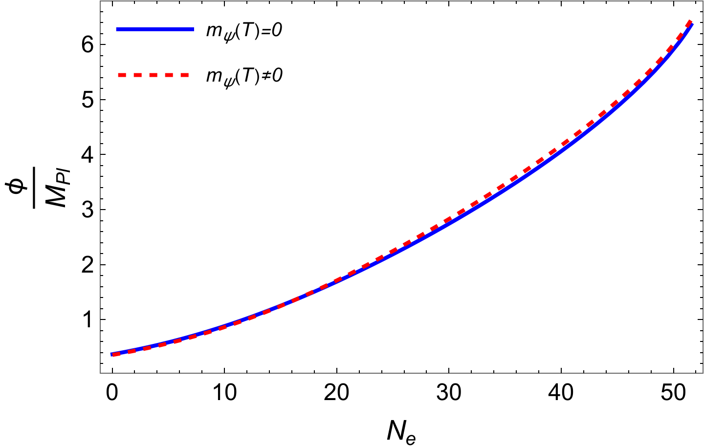
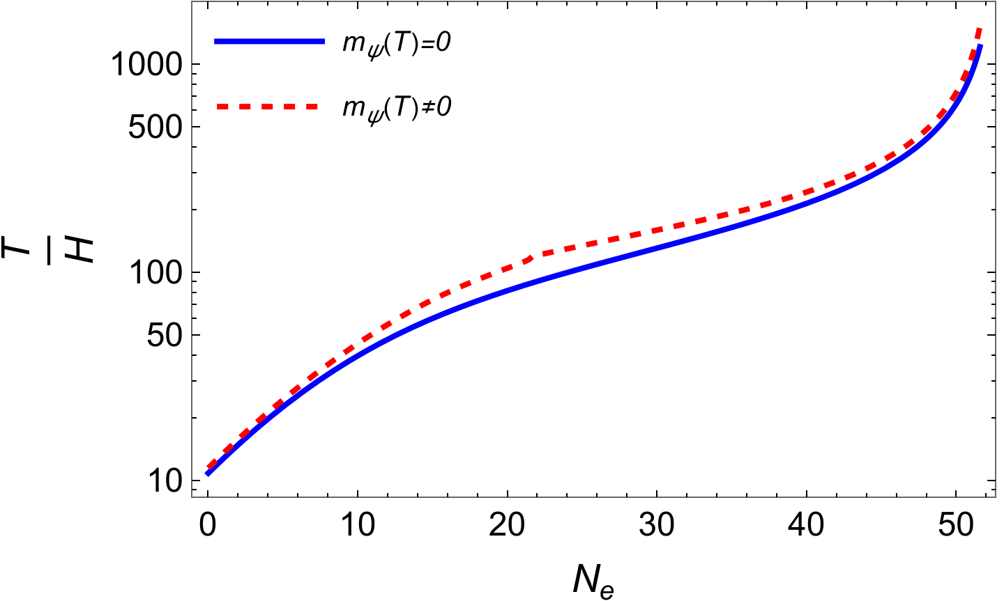
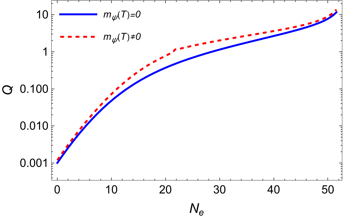
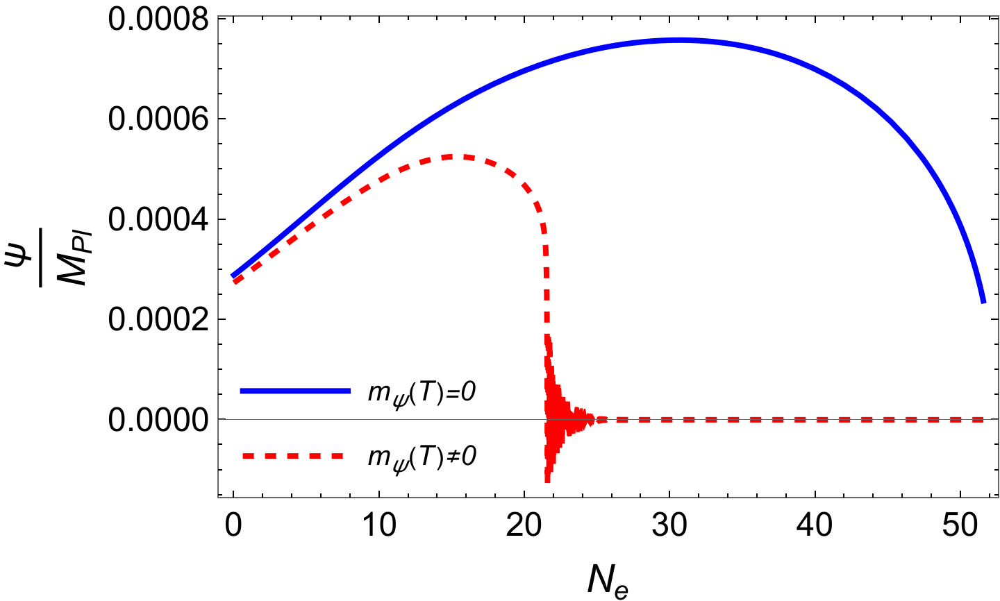
Figure 2: The inflaton field (panel a), temperature over Hubble parameter (panel b), the dissipation ratio $Q=\Upsilon/(3H)$ (panel c) and the gauge field background (panel d) as a function of the number of e-folds. The initial value of the dissipation ratio is $Q_{0}=1.2\times 10^{-3}$. The solid lines correspond to the results obtained in the case where the thermal contribution to the gauge background is neglected, while the dashed lines give the results when it is included.

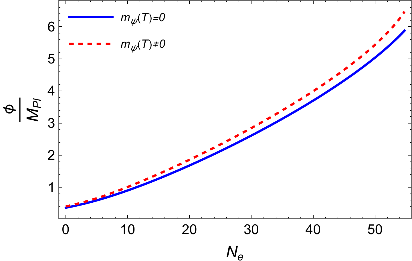
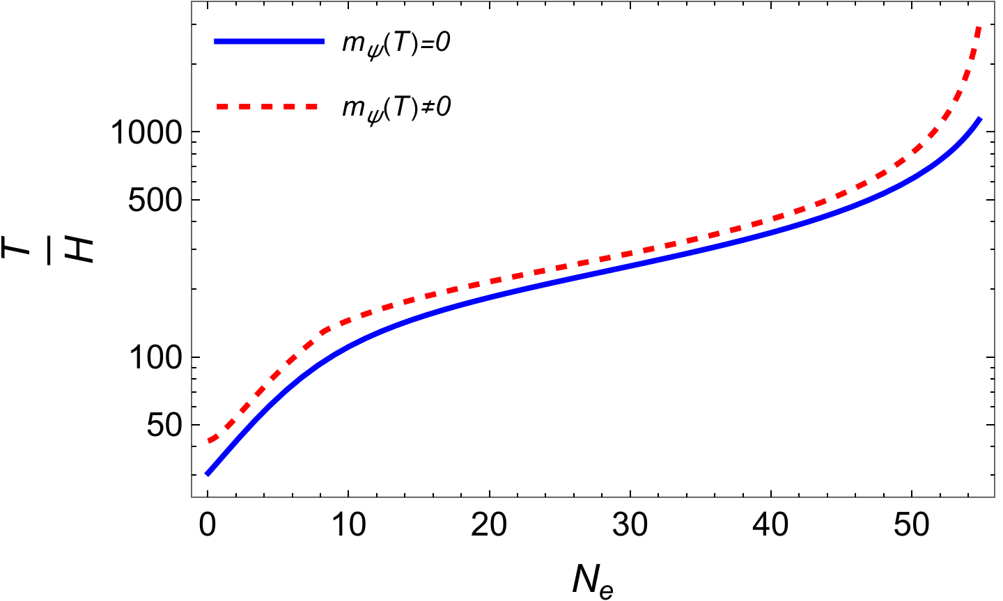
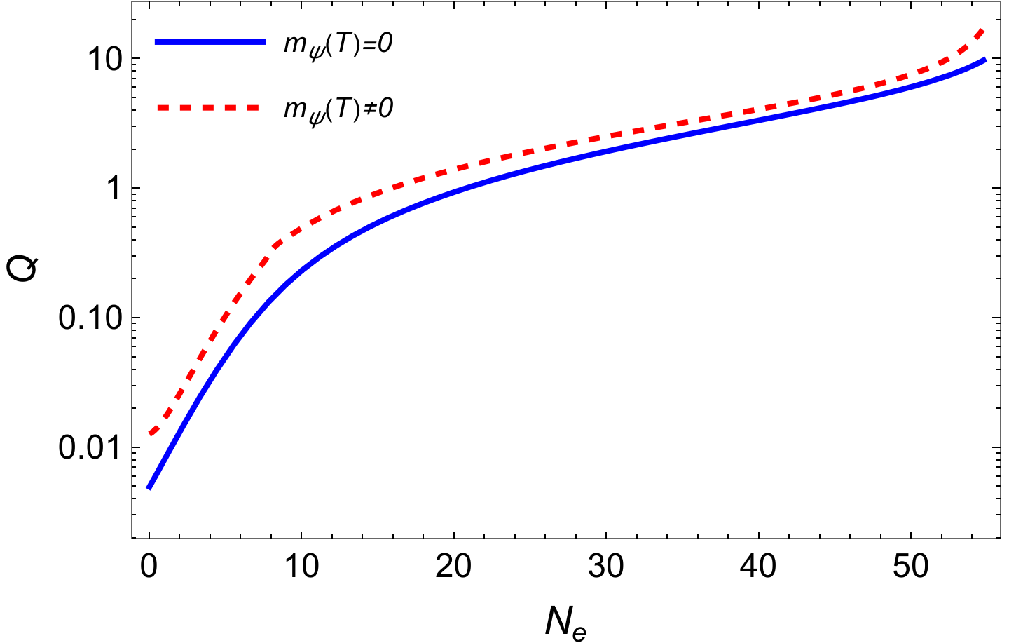
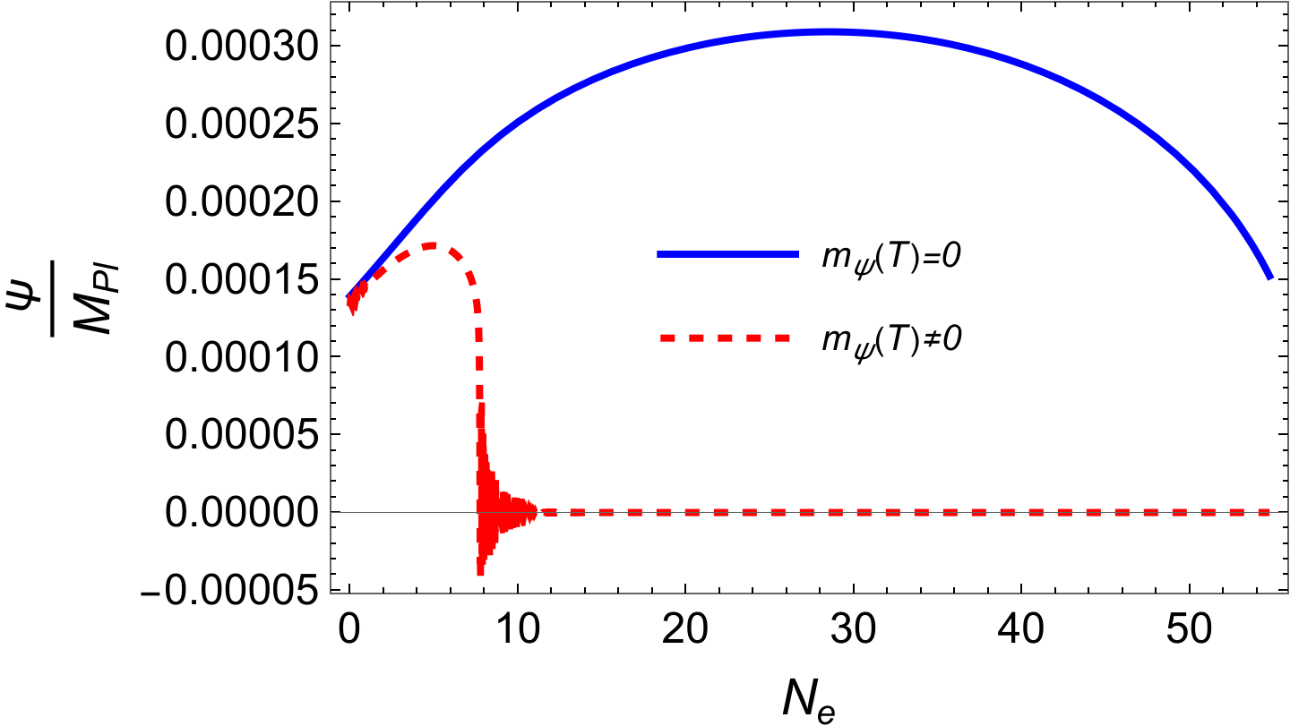
Figure 3: The same as in Fig. 2, but for an initial value of the dissipation ratio is $Q_{0}=1.3\times 10^{-2}$.

To illustrate our results, let us consider an axion-like potential for the inflaton and given by

$$V(\phi)=\Lambda^{4}\left[1+\cos(\phi/f_{D})\right],$$ (45)

where $\Lambda$ is the normalization of the potential (typically $\Lambda^{4}=m_{\phi}^{2}f_{D}^{2}$, where $m_{\phi}$ is the mass of the axion-like particle and $f_{D}$ its decay constant). Note that in standard cold natural inflation one typically requires $f_{D}\gtrsim M_{\rm Pl}/\sqrt{2}$ to have a slowly rolling regime for the inflaton Freese:2004un . To be concrete, we assume $\Lambda$ to correspond to some confinement energy scale of some UV complete theory. Inflation here would then happen at energy scales below $\Lambda$ but still larger than some IR energy scale for the confinement of the $SU(2)$ gauge field considered here, such that the presence of a thermal bath and the use of the dissipation coefficient Eq. (5) are justified.

In warm inflation with a dissipation term like Eq. (5) it was also been shown Montefalcone:2022jfw that consistency of the natural inflation potential with the observations still requires $f_{D}\sim M_{\rm Pl}$. In particular, a more recent analysis Zell:2024vfn has also shown that this model can only sustain inflation consistent with the observations in the weak regime of warm inflation, in which case $Q=\Upsilon/(3H)\ll 1$. Motivated by these previous references, here we will not assume that $f$, which appears in the dissipation and chromoinflation expressions and that comes from the Chern-Simons interaction, and $f_{D}$, which appears in the potential are the same. This will give us some more freedom when playing with the parameters of the model. By fixing $f_{D}$, $\lambda$ and $g$, we can obtain for instance $f$ by demanding to inflation to last a specific number of efolds for a given dissipation ratio $Q$.

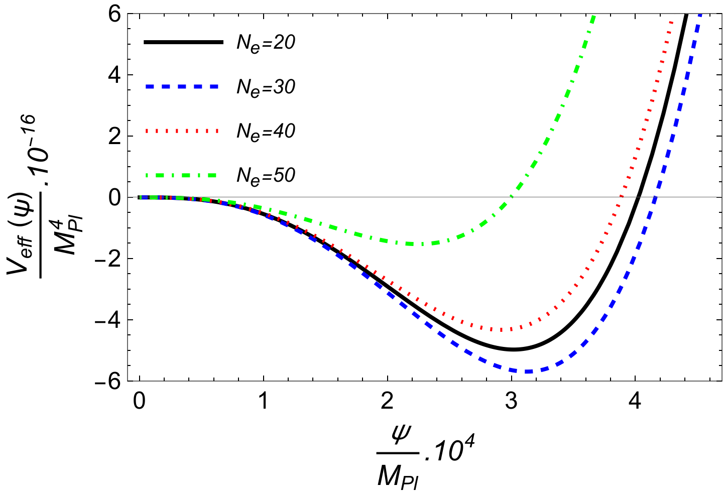
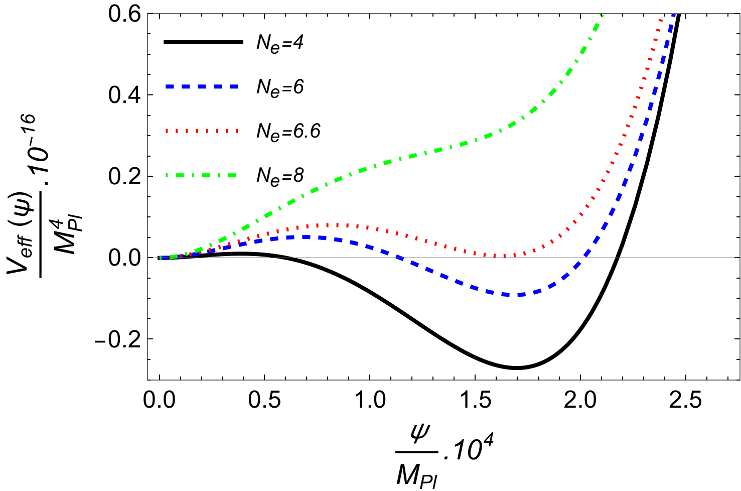
Figure 4: Snapshots of the effective potential Eq. (38) as a function of $\psi$ at specific values of e-folds. Panel (a) is in the absence of the thermal effects for $\psi$, while panel (b) shows the effects of including them.

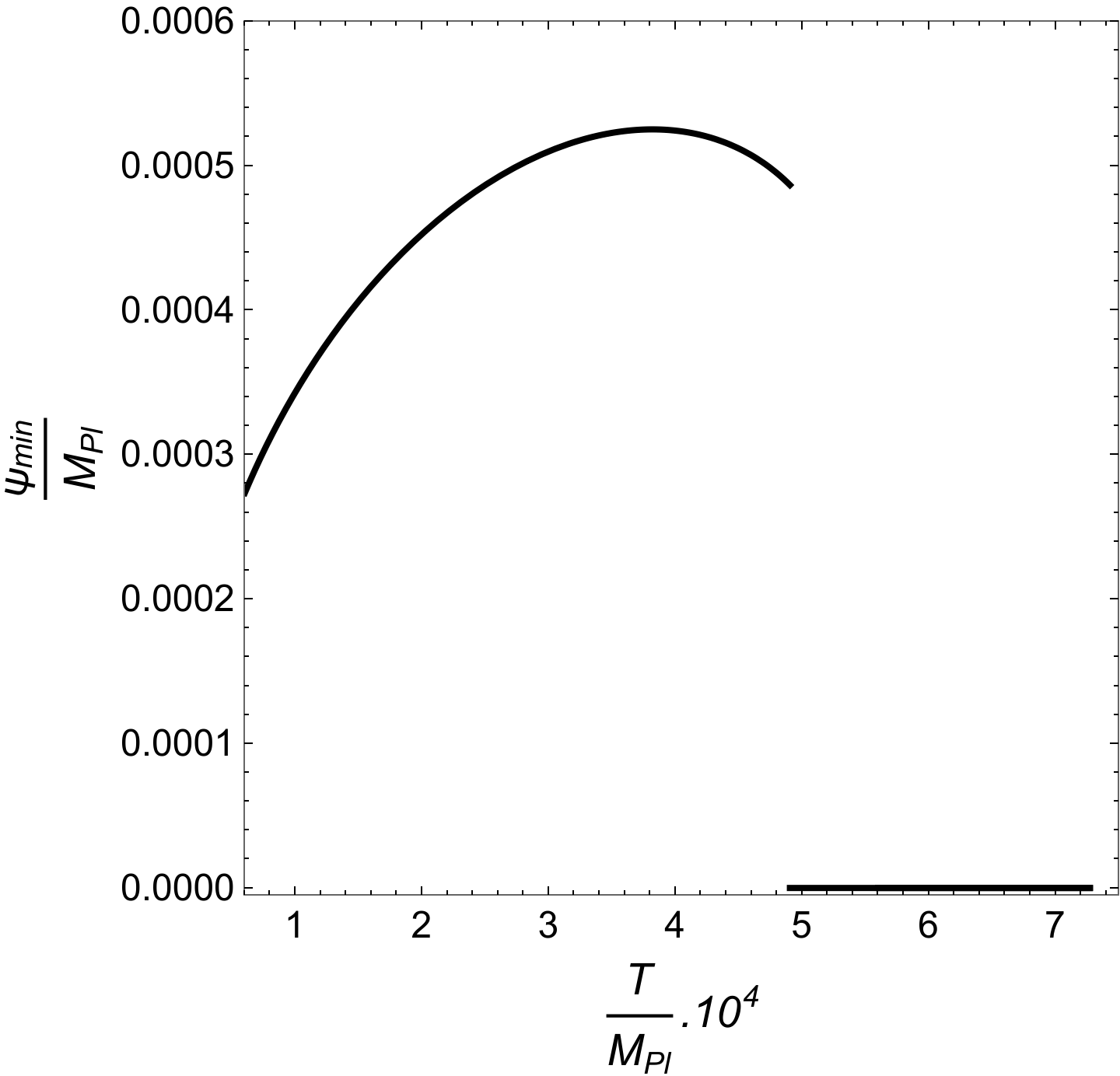
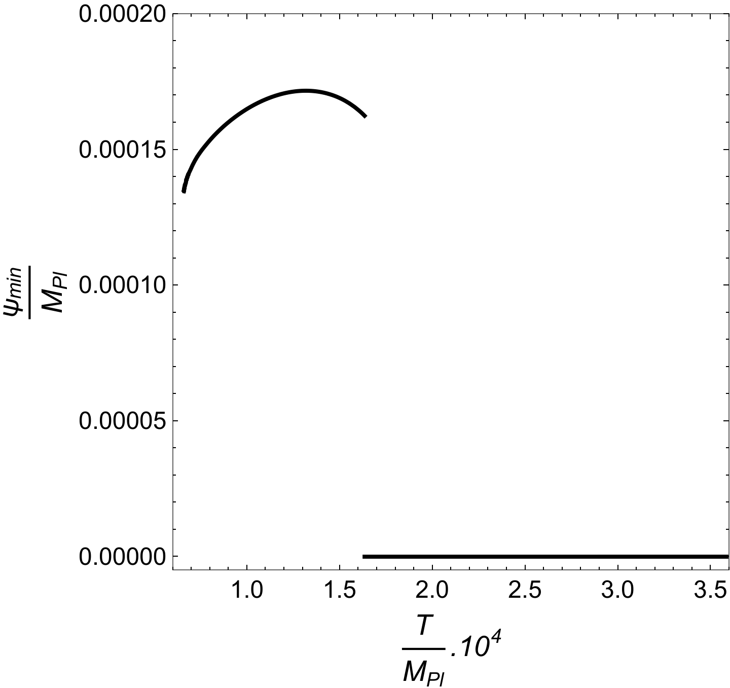
Figure 5: The global minimum of the effective potential Eq. (38) as a function of the temperature, for the cases of $Q_{0}=1.2\times 10^{-3}$ (panel a) and for $Q_{0}=1.3\times 10^{-2}$ (panel b).

Specific examples are given in Figs. 2 and 3, where we show some of the relevant background quantities. In both examples shown in those figures the total number of e-folds of inflation was taken to be $N_{\rm infl}=55$ and for illustration purposes the parameters taken were $g=0.6$, $\lambda=100$, $f_{D}/M_{\rm Pl}=3/\sqrt{2}$ (as motivated e.g. from Ref. Montefalcone:2022jfw ). The initial dissipation ratio in Fig. 2 is $Q_{0}=1.2\times 10^{-3}$, from which the values of $f$ and $\Lambda$ are found to be $f\simeq 0.05M_{\rm Pl}$ and $\Lambda\simeq 0.003M_{\rm Pl}$, respectively. In Fig. 3 we have $Q_{0}\simeq 1.3\times 10^{-2}$, with $f\simeq 0.035M_{\rm Pl}$ and $\Lambda\simeq 0.0016M_{\rm Pl}$.

The results displayed in Figs. 2 and 3 show that the most important effect of including the thermal corrections to the gauge field background is on the evolution of $\psi$ itself. In the absence of a thermal mass correction, the gauge field background is sustained throughout the inflationary evolution. However, in the presence of the thermal correction it is eventually driven to zero well before inflation ends. Furthermore, the larger is the initial value for the dissipation ratio $Q$, the sooner $\psi$ is driven to zero. For the parameters considered, this suppression of $\psi$ already happens in the weak regime of warm inflation, $Q\ll 1$. For the parameters considered and for a dissipation ratio $Q\gtrsim 5\times 10^{2}$, we find that the gauge field background already vanishes at the onset and remains null throughout the inflationary evolution.

In principle, we could believe that the results could be changed by making $g$ very small, thus suppressing the thermal effects and allowing a nonvanishing value for $\psi$ to be sustained throughout inflation. However, this also affects the dissipation coefficient through its dependence on the coupling $g$, forcing either $\lambda$ to be larger or $f$ to be smaller. In general we find that larger values of $Q$ becomes hard to be obtained (we also recall the results of Refs. Montefalcone:2022jfw ; Zell:2024vfn of the difficulties of having warm inflation in the strong regime, $Q>1$, in axion-like inflaton potentials). In special we find that the larger is the dissipation ratio $Q$, one requires smaller couplings to support a gauge background $\psi\neq 0$.

Another approach to favor chromoinflation in the current scenario would be to increase the gauge background field. This would require a gauge field mass, $m_{A}$, much larger than the temperature. This would suppress thermal effects from Eq. (27), as they would be Boltzmann-suppressed. However, this introduces a new challenge. A larger gauge field mass, resulting from a non-zero $\psi$, would also strongly suppress the dissipation coefficient in Eq. (5). This is analogous to what is expected to happen in the electroweak phase transition Cohen:1993nk : above the electroweak scale, massless gauge bosons allow rapid sphaleron processes; below the scale, mass acquisition suppresses these processes. Similarly, here, a larger gauge field mass would suppress the dissipation necessary for warm inflation. While cold chromoinflation could still occur, a warm inflation regime would be precluded.

As discussed at the end of the last section, we can interpret the vanishing of $\psi$ as a true phase transition. This is explicitly illustrate in Fig. 4, where we show snapshots of the effective potential Eq. (38) as a function of $\psi$ at different values of e-folds for the case of $Q_{0}\simeq 1.3\times 10^{-2}$, which is the case shown in Fig. 3. From the results of Figs. 2 and 3 (e.g. from the panels (b) in those figures), this behavior of the minimum of the effective potential can be interpreted in terms of an increasing value of the temperature at the corresponding values of e-folds.

The corresponding critical temperature for the (first-order) phase transition seen in Fig. 4(b) is $T_{c}\simeq 1.6\times 10^{-4}M_{\rm Pl}$, while for the case of the parameters shown in Fig. 1(d), i.e. for $Q_{0}=1.2\times 10^{-3}$ corresponds to $T_{c}\simeq 4.9\times 10^{-4}M_{\rm Pl}$. These values agree well with the simpler estimate given by Eq. (LABEL:Tc). Hence, the smaller is $Q_{0}$, the larger becomes $T_{c}$.

The minimum of the effective potential, corresponding to the solution $\Psi_{+}$ in Eq. (41), as a function of the temperature, is displayed in Fig. 5. It shows the behavior typical of a order parameter as a function of the temperature when the phase transition is first order. The order parameter (which is here represented by $\psi_{+}$) jumps discontinuously from a nonnull to null value across the phase transition point.

V Conclusion

A pseudo-Nambu-Goldstone scalar field coupled to non-Abelian gauge fields via a Chern-Simons term provides a successful model of warm inflation, known as minimal warm inflation. This model arises from the natural dissipation of the axion-like inflaton field due to sphaleron transitions in a thermal bath, ensuring a warm inflationary regime where the temperature $T$ exceeds the Hubble parameter $H$.

Chromoinflation, another model involving axion-like fields coupled to non-Abelian gauge fields, allows for a homogeneous background gauge field. A natural extension is to incorporate this into the minimal warm inflation framework. The thermalized bath of gauge field fluctuations is expected to induce thermal corrections, including a thermal plasma mass, for the background gauge field.

In this paper, we investigated the impact of this thermal mass correction on the background gauge field $\psi$. Our findings reveal that the evolution of $\psi$ can be significantly influenced by thermal effects, particularly at larger dissipation ratios $Q$ characteristic of warm inflation. A non-vanishing initial value of $\psi$ can be rapidly driven to zero by these thermal effects. Subsequently, the dynamics effectively reduces to that of minimal warm inflation without a background gauge field. Conversely, a non-zero gauge field mass, induced by a non-vanishing $\psi$, suppresses sphaleron processes responsible for the dissipation term in Eq. (5). This suppression hinders warm inflation. Therefore, a successful warm inflation scenario in chromoinflation would be prevented.

We have demonstrated that the process by which the background gauge field transitions from a non-zero value to zero closely resembles a phase transition triggered by temperature variations. At a specific critical temperature, the gauge field undergoes a first-order phase transition. We have analytically characterized the properties of this phase transition. We have also illustrated it by an explicit numerical example.

In this work, we have primarily focused on the background dynamics. It is crucial to extend this analysis to perturbations to understand how they differ from standard warm inflation scenarios without a background gauge field. The interplay between the background gauge field and thermal effects could lead to significant deviations. Furthermore, the backreaction effects, commonly studied in cold chromoinflation Maleknejad:2016qjz ; Maleknejad:2018nxz ; Ishiwata:2021yne , should be considered. These additional factors are essential for comparing the model’s predictions with observational data. We plan to address these aspects in a future work.

- (1) A. Berera and L. Z. Fang, Thermally induced density perturbations in the inflation era, Phys. Rev. Lett. 74 (1995), 1912-1915 doi:10.1103/PhysRevLett.74.1912 [arXiv:astro-ph/9501024 [astro-ph]].
- (2) A. Berera, Warm inflation, Phys. Rev. Lett. 75 (1995), 3218-3221 doi:10.1103/PhysRevLett.75.3218 [arXiv:astro-ph/9509049 [astro-ph]].
- (3) A. Berera, M. Gleiser and R. O. Ramos, A First principles warm inflation model that solves the cosmological horizon / flatness problems, Phys. Rev. Lett. 83 (1999), 264-267 doi:10.1103/PhysRevLett.83.264 [arXiv:hep-ph/9809583 [hep-ph]].
- (4) M. Bastero-Gil, A. Berera, R. O. Ramos and J. G. Rosa, Warm Little Inflaton, Phys. Rev. Lett. 117 (2016) no.15, 151301 doi:10.1103/PhysRevLett.117.151301 [arXiv:1604.08838 [hep-ph]].
- (5) M. Bastero-Gil, A. Berera, R. O. Ramos and J. G. Rosa, Towards a reliable effective field theory of inflation, Phys. Lett. B 813 (2021), 136055 doi:10.1016/j.physletb.2020.136055 [arXiv:1907.13410 [hep-ph]].
- (6) K. V. Berghaus, P. W. Graham and D. E. Kaplan, Minimal Warm Inflation, JCAP 03 (2020), 034 [erratum: JCAP 10 (2023), E02] doi:10.1088/1475-7516/2020/03/034 [arXiv:1910.07525 [hep-ph]].
- (7) M. Laine and S. Procacci, Minimal warm inflation with complete medium response, JCAP 06 (2021), 031 doi:10.1088/1475-7516/2021/06/031 [arXiv:2102.09913 [hep-ph]].
- (8) W. DeRocco, P. W. Graham and S. Kalia, Warming up cold inflation, JCAP 11 (2021), 011 doi:10.1088/1475-7516/2021/11/011 [arXiv:2107.07517 [hep-ph]].
- (9) S. Das, Warm Inflation in the light of Swampland Criteria, Phys. Rev. D 99 (2019) no.6, 063514 doi:10.1103/PhysRevD.99.063514 [arXiv:1810.05038 [hep-th]].
- (10) M. Motaharfar, V. Kamali and R. O. Ramos, Warm inflation as a way out of the swampland, Phys. Rev. D 99 (2019) no.6, 063513 doi:10.1103/PhysRevD.99.063513 [arXiv:1810.02816 [astro-ph.CO]].
- (11) S. Das, G. Goswami and C. Krishnan, Swampland, axions, and minimal warm inflation, Phys. Rev. D 101 (2020) no.10, 103529 doi:10.1103/PhysRevD.101.103529 [arXiv:1911.00323 [hep-th]].
- (12) A. Berera and J. R. Calderón, Trans-Planckian censorship and other swampland bothers addressed in warm inflation, Phys. Rev. D 100 (2019) no.12, 123530 doi:10.1103/PhysRevD.100.123530 [arXiv:1910.10516 [hep-ph]].
- (13) V. Kamali, M. Motaharfar and R. O. Ramos, Warm brane inflation with an exponential potential: a consistent realization away from the swampland, Phys. Rev. D 101 (2020) no.2, 023535 doi:10.1103/PhysRevD.101.023535 [arXiv:1910.06796 [gr-qc]].
- (14) A. Berera, R. Brandenberger, V. Kamali and R. O. Ramos, Thermal, trapped and chromo-natural inflation in light of the swampland criteria and the trans-Planckian censorship conjecture, Eur. Phys. J. C 81 (2021) no.5, 452 doi:10.1140/epjc/s10052-021-09240-3 [arXiv:2006.01902 [hep-th]].
- (15) S. Das and R. O. Ramos, Runaway potentials in warm inflation satisfying the swampland conjectures, Phys. Rev. D 102 (2020) no.10, 103522 doi:10.1103/PhysRevD.102.103522 [arXiv:2007.15268 [hep-th]].
- (16) R. Brandenberger, V. Kamali and R. O. Ramos, Strengthening the de Sitter swampland conjecture in warm inflation, JHEP 08 (2020), 127 doi:10.1007/JHEP08(2020)127 [arXiv:2002.04925 [hep-th]].
- (17) M. Motaharfar and R. O. Ramos, Dirac-Born-Infeld warm inflation realization in the strong dissipation regime, Phys. Rev. D 104 (2021) no.4, 043522 doi:10.1103/PhysRevD.104.043522 [arXiv:2105.01131 [hep-th]].
- (18) A. Maleknejad and M. M. Sheikh-Jabbari, Gauge-flation: Inflation From Non-Abelian Gauge Fields, Phys. Lett. B 723 (2013), 224-228 doi:10.1016/j.physletb.2013.05.001 [arXiv:1102.1513 [hep-ph]].
- (19) A. Maleknejad, Axion Inflation with an SU(2) Gauge Field: Detectable Chiral Gravity Waves, JHEP 07 (2016), 104 doi:10.1007/JHEP07(2016)104 [arXiv:1604.03327 [hep-ph]].
- (20) P. Adshead and M. Wyman, Chromo-Natural Inflation: Natural inflation on a steep potential with classical non-Abelian gauge fields, Phys. Rev. Lett. 108 (2012), 261302 doi:10.1103/PhysRevLett.108.261302 [arXiv:1202.2366 [hep-th]].
- (21) V. Kamali, Warm pseudoscalar inflation, Phys. Rev. D 100 (2019) no.4, 043520 doi:10.1103/PhysRevD.100.043520 [arXiv:1901.01897 [gr-qc]].
- (22) A. Maleknejad, M. M. Sheikh-Jabbari and J. Soda, Gauge Fields and Inflation, Phys. Rept. 528 (2013), 161-261 doi:10.1016/j.physrep.2013.03.003 [arXiv:1212.2921 [hep-th]].
- (23) A. Berera, M. Gleiser and R. O. Ramos, Strong dissipative behavior in quantum field theory, Phys. Rev. D 58 (1998), 123508 doi:10.1103/PhysRevD.58.123508 [arXiv:hep-ph/9803394 [hep-ph]].
- (24) J. Yokoyama and A. D. Linde, Is warm inflation possible?, Phys. Rev. D 60 (1999), 083509 doi:10.1103/PhysRevD.60.083509 [arXiv:hep-ph/9809409 [hep-ph]].
- (25) P. Agrawal, J. Fan and M. Reece, Clockwork Axions in Cosmology: Is Chromonatural Inflation Chrononatural?, JHEP 10 (2018), 193 doi:10.1007/JHEP10(2018)193 [arXiv:1806.09621 [hep-th]].
- (26) J. Holland, I. Zavala and G. Tasinato, On chromonatural inflation in string theory, JCAP 12 (2020), 026 doi:10.1088/1475-7516/2020/12/026 [arXiv:2009.00653 [hep-th]].
- (27) G. D. Moore and M. Tassler, The Sphaleron Rate in SU(N) Gauge Theory, JHEP 02 (2011), 105 doi:10.1007/JHEP02(2011)105 [arXiv:1011.1167 [hep-ph]].
- (28) S. Yeasmin and A. Deshamukhya, Effect of dissipation on chromo-natural inflation, Int. J. Mod. Phys. A 38 (2023) no.21, 2350112 doi:10.1142/S0217751X23501129 [arXiv:2203.12213 [astro-ph.CO]].
- (29) A. Mukuno and J. Soda, Chromonatural warm inflation, Phys. Rev. D 109 (2024) no.12, 123504 doi:10.1103/PhysRevD.109.123504 [arXiv:2402.08849 [hep-th]].
- (30) P. Adshead, E. Martinec and M. Wyman, Perturbations in Chromo-Natural Inflation, JHEP 09 (2013), 087 doi:10.1007/JHEP09(2013)087 [arXiv:1305.2930 [hep-th]].
- (31) R. Namba, E. Dimastrogiovanni and M. Peloso, Gauge-flation confronted with Planck, JCAP 11 (2013), 045 doi:10.1088/1475-7516/2013/11/045 [arXiv:1308.1366 [astro-ph.CO]].
- (32) E. Dimastrogiovanni and M. Peloso, Stability analysis of chromo-natural inflation and possible evasion of Lyth’s bound, Phys. Rev. D 87 (2013) no.10, 103501 doi:10.1103/PhysRevD.87.103501 [arXiv:1212.5184 [astro-ph.CO]].
- (33) S. Das, G. Goswami and C. Krishnan, Swampland, axions, and minimal warm inflation, Phys. Rev. D 101 (2020) no.10, 103529 doi:10.1103/PhysRevD.101.103529 [arXiv:1911.00323 [hep-th]].
- (34) M. Srednicki, Quantum field theory, Cambridge University Press, 2007, ISBN 978-0-521-86449-7, 978-0-511-26720-8 doi:10.1017/CBO9780511813917
- (35) J. I. Kapusta and C. Gale, Finite-temperature field theory: Principles and applications, Cambridge University Press, 2011, ISBN 978-0-521-17322-3, 978-0-521-82082-0, 978-0-511-22280-1 doi:10.1017/CBO9780511535130
- (36) T. Fujita, K. Mukaida, K. Murai and H. Nakatsuka, SU(N) natural inflation, Phys. Rev. D 105 (2022) no.10, 103519 doi:10.1103/PhysRevD.105.103519 [arXiv:2110.03228 [hep-ph]].
- (37) N. Goldenfeld, Lectures on Phase Transitions and The Renormalization Group, Frontiers in Physics, Vol. 85 (Addison-Wesley, NY, 1992).
- (38) S. Das and R. O. Ramos, Running and Running of the Running of the Scalar Spectral Index in Warm Inflation, Universe 9 (2023) no.2, 76 doi:10.3390/universe9020076 [arXiv:2212.13914 [astro-ph.CO]].
- (39) K. Freese and W. H. Kinney, On: Natural inflation, Phys. Rev. D 70 (2004), 083512 doi:10.1103/PhysRevD.70.083512 [arXiv:hep-ph/0404012 [hep-ph]].
- (40) G. Montefalcone, V. Aragam, L. Visinelli and K. Freese, Observational constraints on warm natural inflation, JCAP 03 (2023), 002 doi:10.1088/1475-7516/2023/03/002 [arXiv:2212.04482 [gr-qc]].
- (41) S. Zell, No Warm Inflation From Sphaleron Heating With a Vanilla Axion, [arXiv:2408.07746 [hep-ph]].
- (42) D. E. Kaplan and R. Rattazzi, Large field excursions and approximate discrete symmetries from a clockwork axion, Phys. Rev. D 93 (2016) no.8, 085007 doi:10.1103/PhysRevD.93.085007 [arXiv:1511.01827 [hep-ph]].
- (43) K. Choi and S. H. Im, Realizing the relaxion from multiple axions and its UV completion with high scale supersymmetry, JHEP 01 (2016), 149 doi:10.1007/JHEP01(2016)149 [arXiv:1511.00132 [hep-ph]].
- (44) A. G. Cohen, D. B. Kaplan and A. E. Nelson, Progress in electroweak baryogenesis, Ann. Rev. Nucl. Part. Sci. 43 (1993), 27-70 doi:10.1146/annurev.ns.43.120193.000331 [arXiv:hep-ph/9302210 [hep-ph]].
- (45) A. Maleknejad and E. Komatsu, Production and Backreaction of Spin-2 Particles of Gauge Field during Inflation, JHEP 05 (2019), 174 doi:10.1007/JHEP05(2019)174 [arXiv:1808.09076 [hep-ph]].
- (46) K. Ishiwata, E. Komatsu and I. Obata, Axion-gauge field dynamics with backreaction, JCAP 03 (2022) no.03, 010 doi:10.1088/1475-7516/2022/03/010 [arXiv:2111.14429 [hep-ph]].