FISC: Federated Domain Generalization via Interpolative Style Transfer and
Contrastive Learning

Abstract

While Federated Learning (FL) shows promise in preserving privacy and enabling collaborative learning, most current solutions concentrate on private data collected from a single domain. Yet, a substantial problem arises when client data is drawn from diverse domains (i.e., domain shift), leading to poor performance of the trained model on unseen domains. Existing Federated Domain Generalization approaches address this issue but are tailored to scenarios where each client possesses an entire domain’s data. This assumption restricts the practicality of these methods in real-world situations, including domain-based heterogeneity and client sampling. To overcome this limitation, we present FISC, a novel FL domain generalization paradigm designed to handle more complicated domain distributions across clients. FISC facilitates client learning across domains by extracting an interpolative style from local styles obtained from each client and using contrastive learning. This approach provides each client with a multi-domain representation and an unbiased convergent target. Empirical results on multiple datasets, including PACS, Office-Home, and IWildCam, demonstrate FISC’s superiority over state-of-the-art methods. Notably, our method outperforms state-of-the-art techniques by a margin ranging from 3.64 to 57.22% in terms of accuracy on unseen domains. Our code is available at https://anonymous.4open.science/r/FISC-AAAI-16107.

Keywords First keyword  $\cdot$ Second keyword  $\cdot$ More

1 Introduction

Federated learning (FL) McMahan et al. (2017) is a distributed machine learning paradigm that facilitates training a single unified model from multiple disjoint contributors, each of whom may own or control their private data. The security aggregation mechanism and its distinctive distributed training mode render it highly compatible with a wide range of practical applications that have stringent privacy demands Sheller et al. (2020); Nguyen et al. (2021a). Data heterogeneity Li et al. (2020); Karimireddy et al. (2020); Mendieta et al. (2022); Lim et al. (2024) presents a substantial challenge in FL due to the diverse origins of data, each with a distinct distribution. In this scenario, each client optimizes towards the local minimum of empirical loss, deviating from the global direction. Therefore, the averaged global model unavoidably faces a slow convergence speed Li et al. (2020) and achieves limited performance improvement Wang et al. (2020). Many techniques have been developed to handle data heterogeneity in FL Gao et al. (2022); Li et al. (2021); Nguyen et al. (2022a). However, these techniques primarily address label skew — i.e., the variation in label distributions among client’s data within the same domain.

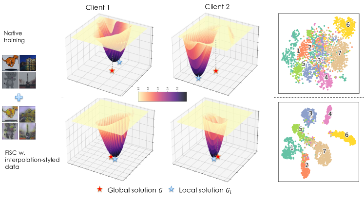
Figure 1: Loss landscape visualization of two clients under domain-based heterogeneity, with normal training (first row) and our method (second row). The vertical axis shows the loss (i.e., solution for the global objective as $G$ and each local objective as $G_{i}$). The horizontal plane represents a parameter space centered at the global model weight. The feature visualization on inter-domains is presented in the last column, which shows that our method acquires generalizing performance on unseen domains.

However, real-world data heterogeneity in practical applications extends beyond class imbalances, introducing complexities such as domain shifts due to the geographical dispersion of data collectors, like cameras and sensors across different hospitals in medical settings Orlando et al. (2020); Guo et al. (2023); Huang et al. (2023). This problem is widely addressed in centralized machine learning, where all training data is collected in central storage. Most existing DG methods for centralized ML Sun and Saenko (2016); Nguyen et al. (2021b); Wang et al. (2021) require sharing the representation of the data across domains or access to data from a pool of multiple source domains (in a central server) Li et al. (2018). However, this violates FL’s privacy-preserving nature and raises a critical need for specialized DG methods in FL.

Recognizing this issue, several Federated Domain Generalization (FedDG) methods have attempted to address domain shift in FL Liu et al. (2021a); Nguyen et al. (2022b); Tenison et al. (2023); Zhang et al. (2023), but their methods and evaluations often reveal several limitations. Firstly, current evaluations are confined to testing on datasets with limited domain diversity and a small number of domains. Secondly, existing approaches are highly sensitive to the number of clients involved in training, and domain-based client heterogeneity Bai et al. (2024) where each client distribution is a (different) mixture of train domain distributions. In addition, client sampling scenarios where only a subset of clients engage are often overlooked, limiting the generalizability of these methods to popular FL setups Fu et al. (2023); Crawshaw et al. (2024). We argue that existing techniques rely on local signals, such as training loss and gradient sign, to mitigate overfitting by penalizing model complexity. However, by treating each client signal as a complete domain indicator, these methods may struggle to generalize when a single client lacks comprehensive domain data. In addition, other methods using cross-sharing local signals, such as amplitude, style statistics, and class-level prototypes, among clients can potentially result in privacy breaches, as discussed in prior studies Nguyen et al. (2022b); Zhang et al. (2023).

To address these challenges, we propose shifting from relying on individual local signals to using an aggregated interpolation style, which fuses shared domain knowledge from all clients. This global interpolation style is formed by clustering and blending local style statistics, creating a representative style that captures common characteristics across domains. By sharing this global style instead of specific local signals, we reduce privacy risks with maintaining superior performance, as the global style conceals client-specific data and class-level information. Given the interpolation style, each client can generate new data that blends local and global domain characteristics. We enforce the model to embed the original data in a manner that is more similar to the style-transferred data from the same class while pushing it away from style-transferred data from other classes. This approach enhances generalization by encouraging the model to focus on domain-invariant features, gradually aligning it with the global model and preventing bias towards local data. Fig. 1 intuitively illustrates local models converge towards its own local optima via loss landscape visualization. Our method aims at guiding local model to optimize towards a converged optimal solution for inter-domain data. This results in better discrimination of unseen domains, as illustrated in the TSNE plot in the Fig. 1’s last column.

We claim the following major contributions in this work.

• We are the first to investigate FedDG methods under both domain-based client heterogeneity and client sampling scenarios, pinpointing the underlying limitation of current methods: the client’s signals in each round is insufficient for representing the complete global domain knowledge, resulting in a model distorted by partial observation.

• We present a novel FedDG method, called FISC, which is robust under domain shift and client-domain heterogeneity. FISC employs unsupervised clustering to identify representative styles across client domains, which are then aggregated into an unbiased interpolative style. Then, we leverage contrastive learning to guide the local model in learning a multi-domain representation aligned with global representation to avoid local bias from their data.

• We rigorously validate the effectiveness of our resulting model with a wide range of datasets (i.e., both small domain and large domain), varied domain distribution and number of client settings. Our results demonstrate that FISC outperforms existing FedDG methods, maintaining comparable computational overhead while effectively preserving client privacy and sensitive information.

2 Methodology

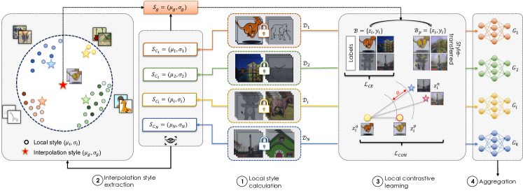
Figure 2: The FISC framework we present in this paper. Clients calculate their style information using their local data and a pre-trained encoder in Step ①. The server extracts interpolation style by weighted averaging the local style information in Step ②. Then, in Step ③, local clients exploit the interpolation style to obtain style-transferred data and update their models via contrastive learning. The aggregated global model in Step ④ runs inference on unseen data.

In this section, we formally introduce the domain-related definitions used in this work and then present FISC, our approach for domain generalization in FL.

2.1 Preliminaries

First, we extend domain and domain generalization definitions in Wang et al. (2022) into domain shift and domain-based client heterogeneity Bai et al. (2023) within the context of FL.

Definition 1 (Domain).

Let $\mathcal{X}$ denote a nonempty input space and $\mathcal{Y}$ an output space. A domain comprises data sampled from a distribution. We denote it as $\mathcal{S}=\left\{\left(\mathbf{x}_{i},y_{i}\right)\right\}_{i=1}^{n}\sim$ $P_{XY}$, where $\mathbf{x}\in\mathcal{X}\subset\mathbb{R}^{d},y\in\mathcal{Y}\subset\mathbb{R}$ denotes the label, and $P_{XY}$ denotes the joint distribution of the input sample and output label. $X$ and $Y$ denote the corresponding random variables.

Definition 2 (Domain Generalization).

We are given $M$ training (source) domains $\mathcal{S}_{\text{train }}=\left\{\mathcal{S}^{i}\mid i=1,\cdots,M\right\}$ where $\mathcal{S}^{i}=\left\{\left(\mathbf{x}_{j}^{i},y_{j}^{i}\right)\right\}_{j=1}^{n_{i}}$ denotes the $i$-th domain. The joint distributions between each pair of domains are different: $P_{XY}^{i}\neq P_{XY}^{j},1\leq i\neq j\leq M$. The goal of domain generalization is to learn a robust and generalizable predictive function $h:\mathcal{X}\rightarrow\mathcal{Y}$ from the $M$ training domains to achieve a minimum prediction error on an unseen test domain $\mathcal{S}_{\text{test }}$ (i.e., $\mathcal{S}_{\text{test }}$ cannot be accessed in training and $P_{XY}^{test}\neq P_{XY}^{i}$ for $\left.i\in\{1,\cdots,M\}\right)$, i.e., $\min_{h}\mathbb{E}_{(\mathbf{x},y)\in\mathcal{S}_{\text{test }}}[\ell(h(\mathbf{x}),y)],$ where $\mathbb{E}$ is the expectation and $\ell(\cdot,\cdot)$ is the loss function.

Definition 3 (Domain Shift in Federated Learning).

We consider a scenario where $M$ training domains $S_{\text{train}}$ are distributed among $K$ participants (indexed by $k$) with respective private datasets $\mathcal{D}_{k}=\left\{(\mathbf{x}_{i}^{k},y_{i}^{k})\right\}_{i=1}^{N_{k}}$, where $N_{k}$ denotes the local data scale of participant $k$. In heterogeneous federated learning, the conditional feature distribution $P(\mathbf{x}|y)$ may vary across participants, even if $P(y)$ remains consistent, leading to domain shift: $P_{k}(\mathbf{x}\mid y)\neq P_{l}(\mathbf{x}\mid y),\text{ where }P_{k}(y)=P_{l}(y).$

Definition 4 (Domain-based Client Heterogeneity).

We consider domain-based client heterogeneity as an instance of domain shift in FL, such that each client distribution $\mathcal{D}_{i}$ is a mixture of training domain distributions, which is $\mathcal{D}_{i}(\mathbf{x},y)=\sum_{d\in\mathcal{S}_{\text{train}}}w_{i,d}\cdot S_{d}(\mathbf{x},y),$ where $w_{i,d}$ represents the proportion of samples from domain $d$ within client $i$.

2.2 FISC: Architecture

Figure 2 presents the overall architecture of FISC. Our method includes four main processes: ① local style calculation, ② interpolation style extraction, ③ contrastive-based local training, and, ④ aggregation. In this subsection, we present how each step is performed. In this work, we adopt the FL scheme formalized from previous works McMahan et al. (2017); Karimireddy et al. (2020), in which all clients agree on sharing a model with the same architecture. We regard the model as having two modules: a feature extractor and a unified classifier. The feature extractor $f:\mathcal{X}\rightarrow\mathcal{Z}$, encodes sample $x$ into a compact $d$ dimensional feature vector $z=f(x)\in\mathbb{R}^{d}$ in the feature space $\mathcal{Z}$. A unified classifier $g:\mathcal{Z}\rightarrow\mathbb{R}^{|I|}$ maps feature $z$ into logits output $y=g(z)$, where $I$ is the classification category.

Local style calculation. Initially, each client must compute their unique style and upload it to the central server. The style information extracted from each local client is carefully abstracted to ensure that it cannot be employed to reconstruct the original dataset. For this purpose, we have chosen to represent the style of each client by statistics of its local data’s feature embedding. Importantly, it has been demonstrated to be highly challenging to reverse-engineer the original dataset solely from this style information ( Chen et al. (2023)). Firstly, to extract the feature representation of each image, we use a pre-trained VGG encoder $\Phi$ of real-time style transfer model AdaIN Huang and Belongie (2017), which will be used to generate interpolative style-transferred data at the next step.

Assume the feature $\Phi(x)$ has the shape of $d\times h\times w$ given channel dimension $x$, in which $h\times w$ is the feature map resolution, and $d$ is the number of dimensions. Then, denote the representation set of a client $\mathcal{C}_{k}$ as $\Phi(\mathcal{C}_{k})$, where $\Phi(\mathcal{C}_{k}):=\{\Phi(x_{i})|\ \forall x_{i}\in\mathcal{D}_{k}\}$. Since each client $k$ may contain data from more than one domain, we cannot estimate precisely the ratio of each domain, i.e., $w_{i,d}$ in Definition 4. Still, we must prevent the local style from being biased by the dominant domains. Therefore, we categorize samples based on different styles using FINCH Sarfraz et al. (2019). This hierarchical clustering method identifies groupings in the data based on its neighborhood relationship without needing hyper-parameters or thresholds. It enables us to discover inherent clustering tendencies inside each client’s samples. Compared to traditional clustering methods, FINCH is more suitable for scenarios where each client contains an uncertain number of clusters. Mathematically, given a set of features $\mathcal{F}$, FINCH outputs a set of partitions $\mathcal{L}=\left\{\Gamma_{1},\Gamma_{2},\cdots,\Gamma_{L}\right\}$ where each partition $\Gamma_{i}=\{C_{1},C_{2},\cdots,C_{\Gamma_{i}}|\ C_{\Gamma_{i}}>C_{\Gamma_{i+1}}\forall i\in\mathcal{L}\}$ is a valid clustering of $\mathcal{F}$, and the last clustering $\Gamma_{L}$ has the smallest number of classes. Here, we use FINCH to group local data points based on their representation $\Phi(\mathcal{C}_{k})$. Specifically,

$$\Phi(\mathcal{C}_{k})\xrightarrow{\text{ FINCH }}\Gamma_{L_{k}}=\left\{\Phi_{j}\right\}_{j=1}^{L_{k}}\in\mathbb{R}^{L_{k}\times d\times w\times h}$$ (1)

This technique implicitly clusters similar characteristic styles due to the low probability of styles from other domains being adjacent. Hence, samples from distinct domains would not successfully combine, whereas those originating from similar domains will be grouped. Specifically, we use cosine similarity to measure the closeness between two image styles and consider the style with the smallest distance as its “neighbor.”

Subsequently, the style of a single cluster $\Phi_{j}\in\mathbb{R}^{d\times w\times h}$ is computed as the pixel-level channel-wise mean and standard deviation feature representation. We denote the style of a cluster $\Phi_{j}$ as $\mathcal{S}_{j}$, then:

$$\mathcal{S}(\Phi_{j})=\left(\mu\left(\Phi_{j}\right),\sigma\left(\Phi_{j}\right)\right)\in\mathbb{R}^{2d}$$ (2)

The local style information for each client $k$ is now the set of all clusters’ styles, i.e., $\mathcal{S}_{\mathcal{C}_{k}}:=\{\mathcal{S}(\Phi_{j})|\forall\Phi_{i}\in\Gamma_{L_{k}}\}$ and the client’s style statistic is then determined by the average of all cluster styles, i.e., $S_{\mathcal{C}_{k}}=\frac{1}{L_{k}}\sum_{i=1}^{L_{k}}\mathcal{S}(\Phi_{i})\in\mathbb{R}^{2d}$.

Interpolation Style Extraction. Since we consider FL settings with many participants and there exists domain-based client heterogeneity among them, we want to find an optimal combination of these local styles, $\mathbf{S}_{\mathcal{C}_{k}}$. Specifically, we use FINCH to find the grouping relationship of these client styles as follows:

$$\mathbf{S}=\left\{\mathcal{S}_{\mathcal{C}_{i}}\right\}_{i=1}^{N}\xrightarrow{\text{ FINCH }}\Gamma_{L}=\left\{\mathcal{S}_{j}\right\}_{j=1}^{L}\in\mathbb{R}^{L\times 2d}$$ (3)

We note that different clients may have overlapping domains or when multiple clients share the same domain. To handle this, we decrease the number of local style representations to $L$ as in Eq. 3 and use the average of each cluster $j$ to represent the style of that cluster. By doing this, the clustering method groups clients with close styles together, and we consider each cluster style equally rather than treating each client equally. Finally, the global interpolation style $\mathcal{S}_{g}$ is defined as the median of all cluster style statistics, i.e., $\mathcal{S}_{g}=median\left(S_{j}\ |\ \forall S_{j}\in\Gamma_{L}\right)\in\mathbb{R}^{2d}$. This enables domains with low cardinality to engage in the interpolation style, hence facilitating the dominant domain’s knowledge acquisition from these smaller populations. The median is robust to outliers (i.e., extreme values) and skewed distributions in style statistics, ensuring no single dominant style skews the global interpolation style. This fairness in representing the central tendency makes the median ideal for capturing diverse client styles without bias, promoting equitable and comprehensive knowledge transfer across all domains.

Local Contrastive Learning. This component demonstrates how each client leverages the global interpolation style, $\mathcal{S}_{g}$, sent from the server to learn an unbiased local model $G_{i}$. The key idea is to use the feature representation of style-transferred data, with the global interpolation style as positive anchors for each data point in $\mathcal{D}_{i}$. Through contrastive learning, the local client learns a feature extractor that aligns its local data and the style-transferred data. Specifically, contrastive learning enhances feature learning by treating samples from the same class with original and transferred styles as positive pairs, and samples from different classes with both styles as negative pairs. This approach fosters more nuanced and discriminative class-level features while enforcing the extraction of domain-invariant features, improving generalization, and reducing biases from domain heterogeneity. To achieve style-transferred data $\mathcal{D}_{i}^{\prime}$ given $\mathcal{D}_{i}$ and $\mathcal{S}_{g}$, we use pre-trained AdaIN model, in which:

$$\operatorname{AdaIN}\left(F_{\mathcal{D}_{i}},\mathcal{S}_{g}\right)=\sigma\left(\mathcal{S}_{g}\right)\left(\frac{f({\mathcal{D}_{i}})-\mu\left(f({\mathcal{D}_{i}})\right)}{\sigma\left(f({\mathcal{D}_{i}})\right)}\right)+\mu\left(\mathcal{S}_{g}\right),$$ (4)

where $f({\mathcal{D}_{i}})$ is the representation of $\mathcal{D}_{i}$ in feature space, and $\mu(.)$ and $\sigma(.)$ are the channel-wise mean and standard variance of image features, respectively. Given a training batch $\mathcal{B}=\{z_{i},y_{i}\}$ with $z_{i},y_{i}$ are the feature representation and label of $i^{th}$ sample, respectively, we denote the corresponding style-transferred batch as $\mathcal{B}_{p}$ such that $\mathcal{B}_{p}=\{\operatorname{AdaIN}\left(z_{i},\mathcal{S}_{g}\right),y_{i}|\ \forall z_{i}\in\mathcal{B}\}$.

To leverage this style-transferred data, we use triplet loss Schroff et al. (2015) to guide clients to learn from embedding following a globally agreed style. In action, for each training batch, FISC would treat all representations of the ground-truth samples as the set of anchors and build up their corresponding positive and negative sets. Specifically, the positive sample for anchor $z_{i}$ is defined as its corresponding style-transferred embedding, i.e., $z^{\prime}_{i}\in\mathcal{B}_{p}$, whereas the negative sample is style-transferred embedding from other classes. Consider the set of negative anchors as: $\textbf{z}_{i}^{n}=\{z_{j}|z_{j}\in\mathcal{B}_{p}\wedge y_{j}\neq y_{i}\}.$ Then, one negative sample $z_{i}^{n}$ will be selected from this set to construct the triplet loss function, which is expressed as follows:

$${\mathcal{L}_{T}}=\sum_{i=1}^{|\mathcal{B}|}\left[\left\|z_{i}^{a}-z_{i}^{p}\right\|_{2}^{2}-\left\|z_{i}^{a}-z_{i}^{n}\right\|_{2}^{2}+\alpha\right].$$ (5)

Here, $z_{i}^{a},z_{i}^{p},z_{i}^{n}$ are feature representations of the current sample $x_{i}$, its positive and negative anchors, respectively, and $\alpha$ is the margin value. Additionally, we incorporate L2 regularization, denoted as $\mathcal{L}_{reg}$, to prevent overfitting and encourage bounded embeddings in contrastive learning. The regularization term is given by:

$$\mathcal{L}_{reg}=\frac{1}{|\mathcal{B}|}\sum_{i=1}^{|\mathcal{B}|}\left(\left(z_{i}^{a}\right)^{2}+\left(z_{i}^{p}\right)^{2}\right)$$ (6)

Including these components in the function ensures a well-balanced and effective contrastive learning process. In addition, we compute CrossEntropy De Boer et al. (2005) loss and use the logits output along with the original annotation signal $\left(y_{i}\right)$ to maintain local domain discriminatory power via: $\mathcal{L}_{CE}=-\mathbf{1}_{y_{i}}\log\left(\sigma\left(g\left(z_{i}\right)\right)\right)$, where $\sigma$ denotes softmax. Finally, each participant $C_{i}$ optimizes on local data during local updating by minimizing the following objective:

$$\mathcal{L}=\mathcal{L}_{CE}+\gamma_{1}\mathcal{L}_{T}+\gamma_{2}\mathcal{L}_{reg}$$ (7)

Aggregation. We adopt the original average aggregator from most FL frameworks, in which the global model $G$ is calculated by $G=\frac{1}{N}\sum_{i=1}^{K}n_{i}G_{i}$, where $n_{i}=|\mathcal{D}_{i}|$ is the data size of client $\mathcal{C}_{i}$ and $N=\sum_{i}^{K}n_{i}$.

3 Experiments

In this section, we compare our method with selected FedDG baselines under FL settings concerning varied training domains, number of clients, and domain-based client heterogeneity, then demonstrate that FISC can achieve improved generalizability in complicated scenarios involving domain-based client heterogeneity and client sampling. We conduct all the experiments using PyTorch version 2.1.0 Imambi et al. (2021) and use the framework provided by Bai et al. (2024) to simulate a domain-based client heterogeneity. We present the key results below and leave more discussion and detailed settings in the Appendix. All experiments are run on a computer with an Intel Xeon Gold 6330N CPU and an NVIDIA A6000 GPU.

3.1 Experimental Setup

Table 1: Comparison of inter-domain performance with SOTA methods under different split LTDO schemes, i.e., two domains are used for validation. AVG denotes the average accuracy calculated from each domain. (The best average accuracy is marked in bold-underline. The second-best average accuracy is marked in underline.)

		Validation Accuracy					Test Accuracy
Dataset	Methods	A	P	C	S	AVG	P	S	A	C	AVG
PACS	FedSR	14.80%	14.67%	13.39%	13.36%	14.06%	13.80%	13.97%	14.55%	12.87%	13.80%
	FedGMA	39.31%	94.13%	63.95%	36.22%	58.40%	73.83%	64.85%	73.10%	52.73%	66.13%
	FPL	77.93%	94.49%	64.97%	31.61%	67.25%	93.53%	55.97%	62.01%	51.83%	65.84%
	FedDG-GA	64.99%	92.46%	63.18%	32.73%	63.34%	84.19%	63.55%	61.87%	48.08%	64.42%
	CCST	68.51%	96.41%	59.26%	35.68%	64.97%	86.89%	59.91%	71.78%	50.94%	67.38%
	Ours	73.63%	95.57%	69.41%	35.91%	68.63%	93.05%	66.20%	71.73%	53.11%	71.02%
		C	A	R	P	AVG	A	P	C	R	AVG
OfficeHome	FedSR	1.40%	1.24%	1.36%	1.31%	1.33%	1.15%	1.14%	1.34%	1.33%	1.24%
	FedGMA	43.18%	54.92%	66.81%	54.29%	54.80%	55.71%	66.43%	39.91%	56.83%	54.72%
	FPL	45.72%	56.82%	69.45%	46.18%	54.54%	59.95%	65.22%	43.99%	52.54%	55.43%
	FedDG-GA	38.99%	51.38%	63.85%	48.07%	50.57%	51.63%	62.38%	36.68%	54.79%	51.37%
	CCST	44.81%	52.48%	62.29%	49.85%	52.36%	52.20%	62.79%	38.37%	54.88%	52.06%
	Ours	46.74%	58.84%	71.13%	55.31%	58.01%	60.09%	67.54%	45.41%	61.62%	58.67%
	PACS: A: Art-Painting, P: Photo, C: Cartoon, S: Sketch
	OfficeHome: C: Clipart, A: Art, R: Real World, P: Product

Table 2: Performance (%) comparisons with the start-of-the-art FedDG methods with the PACS dataset under LODO schemes, i.e., one domain is left for validation.

Methods	PACS					OfficeHome
	P	A	C	S	AVG	P	A	C	R	AVG
FedSR	14.01%	13.27%	15.66%	13.49%	14.11%	1.14%	1.27%	1.34%	1.68%	1.36%
FedGMA	91.08%	81.25%	66.04%	61.72%	75.02%	69.99%	61.60%	49.87%	71.93%	63.35%
FPL	98.20%	81.98%	69.41%	62.64%	78.06%	68.98%	63.00%	48.98%	71.24%	63.05%
FedDG-GA	97.19%	76.17%	58.67%	53.42%	71.36%	66.03%	41.49%	45.98%	64.22%	54.34%
CCST	97.07%	84.18%	72.44%	59.43%	78.28%	66.93%	56.82%	47.35%	69.11%	60.05%
Ours	97.78%	83.89%	73.04%	66.76%	80.37%	71.14%	62.22%	50.70%	73.35%	64.35%

Datasets. We evaluate our methods on three diverse classification tasks, each represented by a specific dataset. The first dataset is PACS Li et al. (2017), encompassing four distinct domains: Photo (P), Art (A), Cartoon (C), and Sketch (S). PACS comprises a total of 7 classes. The second dataset, Office-Home Venkateswara et al. (2017), involves four domains with 65 classes. The four domains are Art, Clipart, Product, and Real-World. The third dataset is IWildCam Koh et al. (2021), a real-world image classification dataset based on wild animal camera traps worldwide, where each camera represents a domain. It contains 243 training, 32 validation, and 48 test domains with a total of 182 classes.

FL Simulation. Based on the framework provided by Bai et al. (2024), we simulate an FL system with a total of $N$ clients; in each training round, the server will randomly select $k\%$ of clients to participate, which is known as client sampling. The data distribution of each client is simulated by domain-based client heterogeneity by $\lambda$ level. We establish a rigorous FL scenario by adjusting the ratio of participating clients $k$ to total clients ($k$/$N$) and heterogeneity degree ($\lambda$). Unless otherwise noted, our default parameters are $N=100$ and $k=20\%$ for PACS/Office-Home, and $N=243$ and $k=10\%$ for IWildCam, with a heterogeneity level of $\lambda=0.1$. We set the number of communication iterations to 50 rounds for PACS/OfficeHome and 100 for IWildCam, and the number of local training epochs to 1. The batch size is set to $32$ for all three datasets.

Baselines. We compare ours against five SOTA methods focusing on addressing domain generalization in FL, representative of three FedDG approaches in related works.

3.2 Experimental Results

Comparison with State-of-the-Art. First, we evaluate FedDG methods under different validation schemes by varying the domain(s) used for training. Specifically, we consider two evaluation methods: Leave-One-Domain-Out (LODO) Nguyen et al. (2022b); Huang et al. (2023) and Leave-Two-Domains-Out (LTDO) Bai et al. (2024) with PACS and OfficeHome datasets.

LTDO Scenarios. Table 1 shows the final accuracy measurements with popular SOTA methods by the end of the FL process. We leave out two domains in each scheme alternately for validation and test accuracy. These results suggest that FedSR is not well-suited in scenarios where each client contains a small amount of data (e.g., with a large number of clients), which aligns with observations in previous work Bai et al. (2024). Other methods, such as FedGMA, FPL, and CCST, can somewhat generalize the FL model, but show degradation when training on domains less representative of the unseen domain, such as training on Photo and testing on Cartoon. On the other hand, our method performs substantially better than other methods, confirming that it generalizes well and thus effectively boosts performance on different unseen domains. Significantly, in the best case, our method outperforms with a gap of 3.64% compared to the second-best method for the PACS dataset.

LODO Scenarios. Table 2 presents the accuracy of compared methods with LODO experiments, i.e., we leave one domain out and use three domains for training. Generally, all methods achieve higher accuracy when more domains are used for training. Our method consistently performs best with PACS and OfficeHome datasets by achieving an average of 80.37% and 64.35% accuracy. Especially with domains such as Cartoon and Sketch of PACS dataset, we observe a large gap between our method and other baselines; our method outperforms the second-best method (i.e., FPL) by 4.63% and 4.12%, respectively.

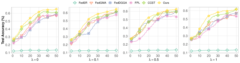
Figure 3: Convergence curve when training round increases on PACS’s Sketch, and training domains are Art-Painting and Cartoon; decreasing domain heterogeneity from left to right. $\lambda=0$ means domain separation while $\lambda=1.0$ means homogeneous domain distribution.

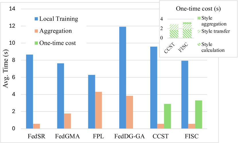
Figure 4: Computational overhead of FedDG methods.

Impact of Domain Heterogeneity. This experiment aims to study the effectiveness of different methods with different domain distribution settings. As shown in Figure. 4, the larger the value of $\lambda$ is, the more heterogeneous domain distribution is among clients. We observe the accuracy when varying the domain heterogeneity using $\lambda=\left\{0.0,0.1,0.5,1.0\right\}$ values. Figure. 4 shows that our method consistently outperforms other baselines under varied domain heterogeneity. Interestingly, our method also achieves the highest accuracy early in training, creating a substantial gap over other baselines.

Next, we consider IWildCam, a dataset containing a larger number (323) of domains. Most SOTA methods demonstrate degraded accuracy. In particular, when $\lambda=0.0$, there is no domain overlap between clients, and the local models quickly converge to a biased model. The second-based performer, CCST, is demonstrably weaker in this challenging case. Our method notably demonstrates robustness by achieving the best average accuracy on validation and testing sets.

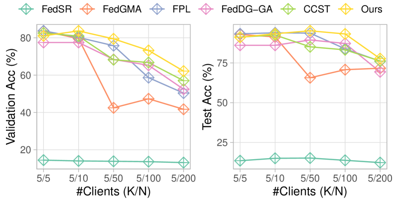
Figure 5: Accuracy comparison with different settings of selected clients (K) per total number of clients (N).

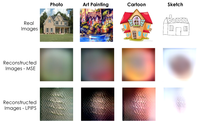
(a) Reconstructed images

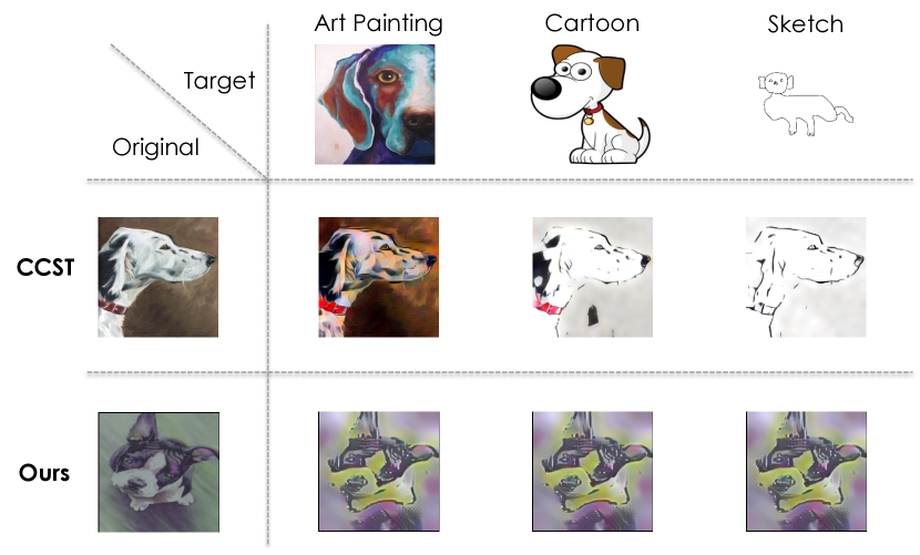
(b) Style-transferred images

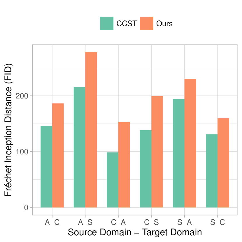
(c) FIDs comparison

Figure 6: The reconstructed images from a GAN model using the client’s style in Fig. 6a, and comparison of style-transferred images from ours and cross-client style transfer in Figs. 6b and 6c.

Table 3: Accuracy (%) comparisons after 100 training rounds of the different methods with the IWildCam dataset, whose 243 training, 32 validation, and 48 test domains.

	Validation Accuracy				Testing Accuracy
Methods	$\lambda=0.0$	$\lambda=0.1$	$\lambda=1.0$	AVG	$\lambda=0.0$	$\lambda=0.1$	$\lambda=1.0$	AVG
FedSR	3.12%	32.97%	5.57%	13.89%	1.87%	16.04%	2.76%	6.89%
FedGMA	39.26%	72.47%	74.65%	62.13%	16.14%	61.21%	59.45%	45.60%
FPL	45.61%	70.45%	72.44%	62.83%	38.71%	54.29%	60.07%	51.02%
FedDG-GA	37.33%	67.98%	71.72%	59.01%	34.97%	59.29%	56.85%	50.37%
CCST	20.89%	66.20%	70.62%	52.57%	38.01%	56.58%	58.95%	51.18%
Ours	54.26%	67.69%	73.55%	65.17%	44.03%	57.23%	60.58%	53.95%

Impact of Number of Clients. The stability of different methods in federated learning (FL) depends on the number of clients, which can range from small (around ten) to large (hundreds or thousands). In many FL schemes, the server randomly selects $K$ participants from a total of $N$ in each training round, especially with many participants. We consider five cases: $N\in\{5,10,50,100,200\}$ and $K=5$, which correspond to 100%, 50%, 10%, 5%, 2.5% clients participating in each round, respectively. We present the comparison of different methods in Figure. 5. The higher the ratio of $K/N$ is, the larger the amount of data participating in each training round is. The scenario of $5/5$ is the most similar setting to previous work, i.e., the number of clients is small, and all clients join each training round. While other methods, such as FPL and CCST, exhibit strong performance with a small number of clients, their efficacy diminishes with an increase in the total number of clients. In contrast, our method outperforms in terms of stability and efficiency.

Computational Overhead. As presented in Fig. 4, the average computation time of FISC is comparable or even smaller than other baselines: (i) FISC does not introduce additional overhead during aggregation, which linearly increases with respect to training rounds as in FedDGGA, FedGMA or FPL. The overhead of average local training is comparable to other methods. The cost for interpolation style calculation is a one-time cost, happening before the training and only takes 3.3s, while the general local training takes 8.67s on average for all methods. This one-time cost does not increase linearly with the number of clients since all clients can conduct local style extraction simultaneously, and the clustering on the server is fast (only 0.3s). Therefore, FISC introduces low overhead when applied to large-scale systems.

Security Analysis. First, we conduct experiments to assess the potential of third-party/server reconstruction attacks — i.e., if an adversary compromises the style vectors and wants to reconstruct private training images from the shared style vectors using generative models Liu et al. (2020). The result shows that the reconstructed images (Fig. 6a) are far different from the real images. We conclude that it is non-trivial to reconstruct a client’s data using only style vectors as in our approach. This observation is aligned with Chen et al. (2023). Second, we demonstrate that interpolation style transfer offers stronger privacy protection than cross-local style transfer by comparing our generated images to those from CCST Chen et al. (2023). As visualized in Fig. 6b, the images produced by FISC across different target domains are visually indistinguishable. We further quantify the similarity between the original private images and the reconstructed ones using Fréchet Inception Distance (FID) Heusel et al. (2017); Seitzer (2020), where a lower FID implies closer resemblance to the original, and a higher FID indicates stronger privacy preservation. As shown in Fig. 6c, our method consistently achieves higher FIDs across all target domains, suggesting that FISC-generated images are far less informative to potential adversaries than those from CCST. In conclusion, FISC provides superior privacy protection compared to cross-client sharing mechanisms, and the use of style statistics does not introduce additional security risks.

4 Related Work

Domain Generalization. Domain generalization aims to learn a model from multiple source domains so that the model can generalize to an unseen target domain. Existing work has explored domain shifts from various directions in a centralized data setting. These methods can be divided into three categories Wang et al. (2022), including data manipulation to enrich data diversity Shankar et al. (2018); Zhou et al. (2021), domain-invariant feature distribution across domains for the robustness of conditional distribution to enhance the generalization ability of the model Nguyen et al. (2021b); Mitrovic et al. (2021), and exploiting general learning strategies such as meta-learning-based Niu et al. (2023) and transfer learning Zhang et al. (2022) to promote generalizability.

However, many of these methods require centralized data from different domains, violating local data preservation in federated learning. Specifically, access for more than one domain is needed to augment data or generate new data in Shankar et al. (2018); Shi et al. (2022); domain-invariant representation learning or decomposing features are performed under the comparison across domains and some learning strategy-based methods use an extra domain for meta-update Arjovsky et al. (2019); Piratla et al. (2020). There exists some methods that do not explicitly require centralized domains and can be adapted for federated learning with minor adjustments. However, these methods such as MixStyle Zhou et al. (2021),Xu et al. (2021) and JiGen Carlucci et al. (2019) offer minimal improvement in addressing domain shift in FL due to constrained intra-client and differing inter-client distributions, as noted by Chen et al. (2023); Bai et al. (2024). This highlights the preference for a specialized FedDG method that preserves the distributed nature of FL while efficiently enhancing generalizability.

Federated Domain Generalization. Existing works tackling heterogeneity among clients in FL Hanzely et al. (2020); Karimireddy et al. (2020); Qu et al. (2022) have not considered model performance under the domain shift between training and testing data. Recently, works tackling DG in FL Liu et al. (2021a); Nguyen et al. (2022b); Huang et al. (2023); Zhang et al. (2023); Tenison et al. (2023); Chen et al. (2023) have been proposed. First, cross-information sharing lets other clients see information abstracted from one client’s domain — for example, the amplitude spectrum Liu et al. (2021a); Shenaj et al. (2023) and the representation statistics Chen et al. (2023). Other clients then use this information to produce synthetic data that contains domain information to enrich the local data. However, these methods cause additional costs and risks of data privacy leakage since the style information of each client is publicly available to other clients. Second, multi-object optimization aligns the generalization gaps among clients. For example, Zhang et al. (2023) create a new optimization goal with a regularizer to lower variance and get a tighter generalization bound. Nguyen et al. (2022b) proposed restricting the representation’s complexity to help minimize the distribution distance between specific and reference domains. In Tenison et al. (2023), the authors suggested using a gradient-masked averaging aggregation method based on the signed agreement of the local updates to eliminate weight parameters with much disagreement. Besides these two approaches, third, unbiased learning Huang et al. (2023) improves domain generalization by creating unbiased by-class prototypes and using regularization to line up the local models with the unbiased prototypes. However, previous studies on FedDG have often focused on domain-isolated settings where the number of clients equals the number of training domains. In addition, these methods shows limited effectiveness under more complicated scenarios such as domain-based heterogeneity and datasets with large number of domains Bai et al. (2024). Moreover, client sampling, – a common setting in FL Fu et al. (2023); Crawshaw et al. (2024), is normally overlooked, where only a portion of clients participate in each training round. Unlike prior methods, we relax the assumption of isolated domain distribution by considering various client-domain heterogeneity and client sampling scenarios. We argue that efficient FedDG methods have to perform robustly and securely under these settings with reasonable computation cost.

5 Conclusions

This work presents FISC, a domain generalization method for Federated Learning. FISC extracts an unbiased interpolative style from all clients to facilitate style transfer. Each client then performs style transfer using this information through contrastive learning, aiming to enhance generalizability and mitigate local bias. Consequently, the aggregated model achieves improved accuracy for unseen domains. Extensive experiments showcase FISC’s superior performance over existing FL Domain Generalization baselines across various settings, including small to large domain datasets and domain heterogeneity scenarios. In addition, using an interpolation style helps enhance the local privacy of clients compared to a cross-client style’s information exchange mechanism.

Appendix / supplemental material

The code is publicly available here: https://anonymous.4open.science/r/FISC-AAAI-16107

Appendix A Experimental Settings

A.1 Datasets

In this section, we introduce the datasets we used in our experiments, the split method we used to build heterogeneous datasets in the training and testing phase, and the heterogeneous local training datasets among clients in the FL.

• PACS Li et al. [2017]: PACS is an image dataset for domain generalization. It consists of four domains, namely Photo (1,670 images), Art Painting (2,048 images), Cartoon (2,344 images), and Sketch (3,929 images). Each domain contains seven categories. This dataset includes 7 classes (Dog, Elephant, Giraffe, Guitar, Horse, House, Person).

• Office-Home Venkateswara et al. [2017]: The Office-Home dataset has been created to evaluate domain adaptation algorithms for object recognition using deep learning. It consists of images from 4 different domains: Art (2,427 images), Clipart (4,365 images), Product (4,439 images), and Real-World (4,357 images). The dataset contains images of 65 object categories with 15,500 images.

• IWildCam Koh et al. [2021]: The IWildCam 2022 training set contains 201,399 images with a total of 182 classes from 323 locations, which are further divided into 243 training domains, 32 validation and 48 test domains. Each location is considered a domain since the camera’s different configurations are associated, resulting in different image quality. This dataset is challenging because of various factors such as illumination, motion blur, occlusion, etc.

A.2 Experimental setup

A.2.1 Training’s hyperparameters

In this section, we present the hyperparameters selected for the evaluation. In the FL simulation, we run 50 communication rounds for PACS and Office-Home and 100 rounds for IWildCam. In each round, the server randomly samples $K$ among $N$ clients to participate in the training. Each selected client will then train their local model using their private data for a specific number of epochs. We use ResNet-50 He et al. [2016] with Adam optimizer for all experiments regarding model architecture and optimizer. After completing all communication rounds, the global model will be tested on unseen domains. Please refer to Table 4 to review training hyper-parameters.

Table 4: Hyper-parameters for simulating FL training

Dataset	Train batch size	Test batch size	Optimizer Learning rate	# Local training epoches	Model architecture	# Clients (K/N)	# Communication rounds
PACS	32	512	Adam $3\times 10^{5}$	1	ResNet-50	20/100	50
Office-Home	32	512	Adam $3\times 10^{5}$	1	ResNet-50	20/100	50
IWildCam	32	512	Adam $3\times 10^{5}$	1	ResNet-50	24/243	100

A.2.2 Dataset split setup

Domain-based heterogeneity degree $\lambda$. We construct Heterogeneous Partitioning $\left\{\mathcal{P}_{\lambda}\right\},\lambda\in[0,1]$, to simulate domain-based heterogeneity, followed by Bai et al. [2024]. It is parameterized by $\lambda$, which allows for the generation of Complete Heterogeneity ($\lambda=0$) and ensures that True Partition is always satisfied (for all $\lambda\in[0,1]$) by design. Additionally, it strives to achieve the optimal balance within these constraints. Heterogeneous Partitioning enables the allocation of samples from multiple domains across any number of clients $C$, with the degree of domain-based client heterogeneity controlled by the parameter $\lambda$, spanning from homogeneity to complete heterogeneity. The 0 value of $\lambda$ means domain separation, and there is no domain overlapping if the number of domains is larger or equal to the total number of clients, i.e., $|\mathcal{D}|\geq N$. The larger the value of $\lambda$ is, the more homogeneous the domain distribution is.

For each dataset, we first split the dataset into five categories: training dataset, in-domain validation dataset, in-domain test dataset, held-out validation dataset, and test domain dataset. For the experiment with LODO, we select a combination of each of the two domains as the training, which ends up in four scenarios: (Cartoon, Sketch), (Art Painting, Cartoon), (Photo, Sketch) and (Photo, Art Painting). In each scenario, the remaining two domains are used for testing. Similarly, there are four scenarios for Office-Home, including (Art, Clipart), (Clipart, Real-World), (Product, Art), and (Product, Real-World). For the training domain, we split 10%, 10% of the total training domain datasets as the in-domain validation dataset and in-domain test dataset, respectively. For IWildCam, we directly apply the Wilds official splits. The visualization of domain distribution among clients in FL with PACS dataset under different values of $\lambda$ is visualized in Fig. 7. In addition, we visualize the domain distribution of the large-domain IWildCam dataset in Fig. 8.

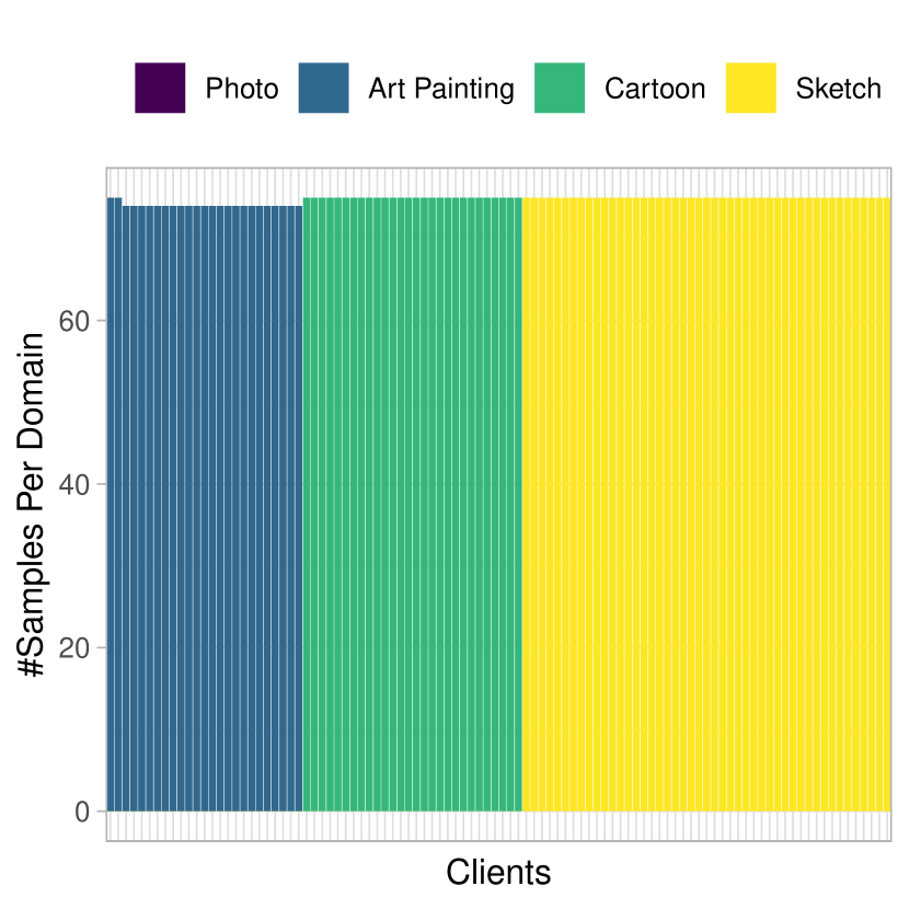
(a) $\lambda=0.0$

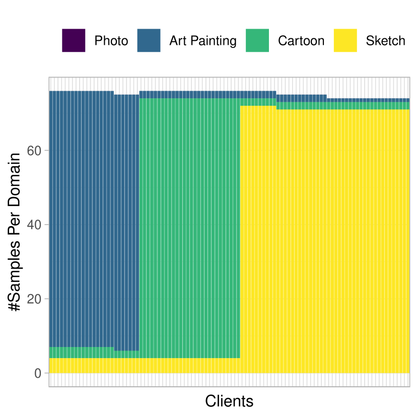
(b) $\lambda=0.1$

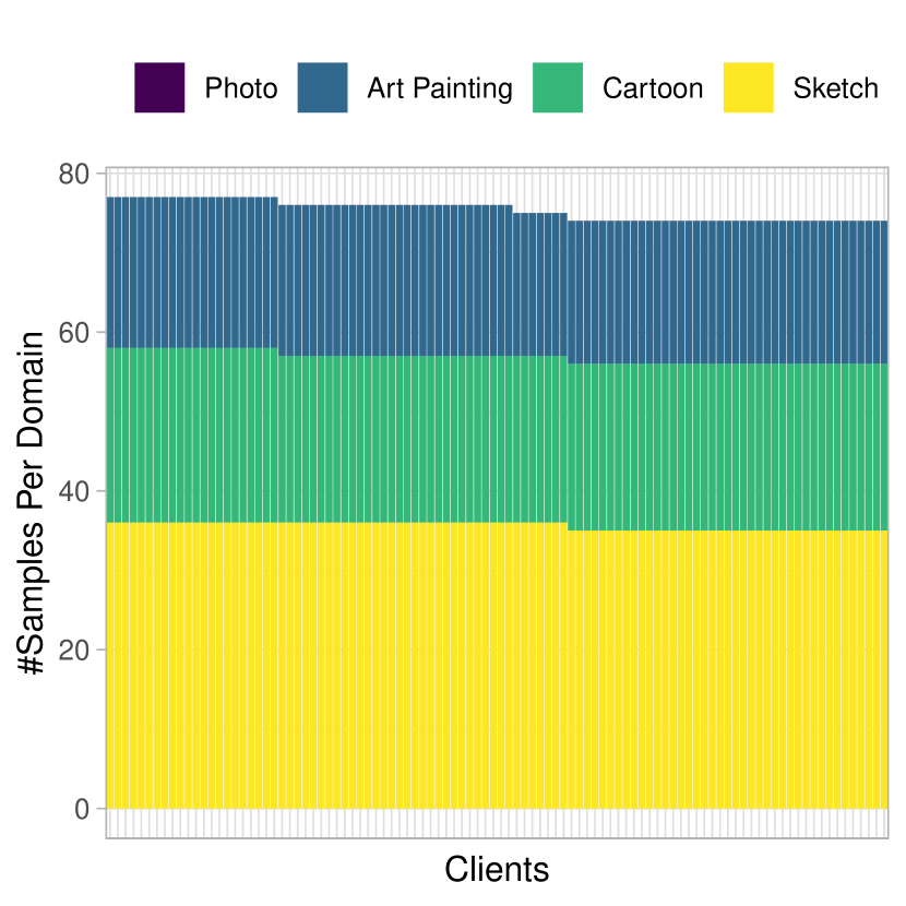
(c) $\lambda=1.0$

Figure 7: Client’s domain heterogeneity distribution illustrated for the PACS dataset.

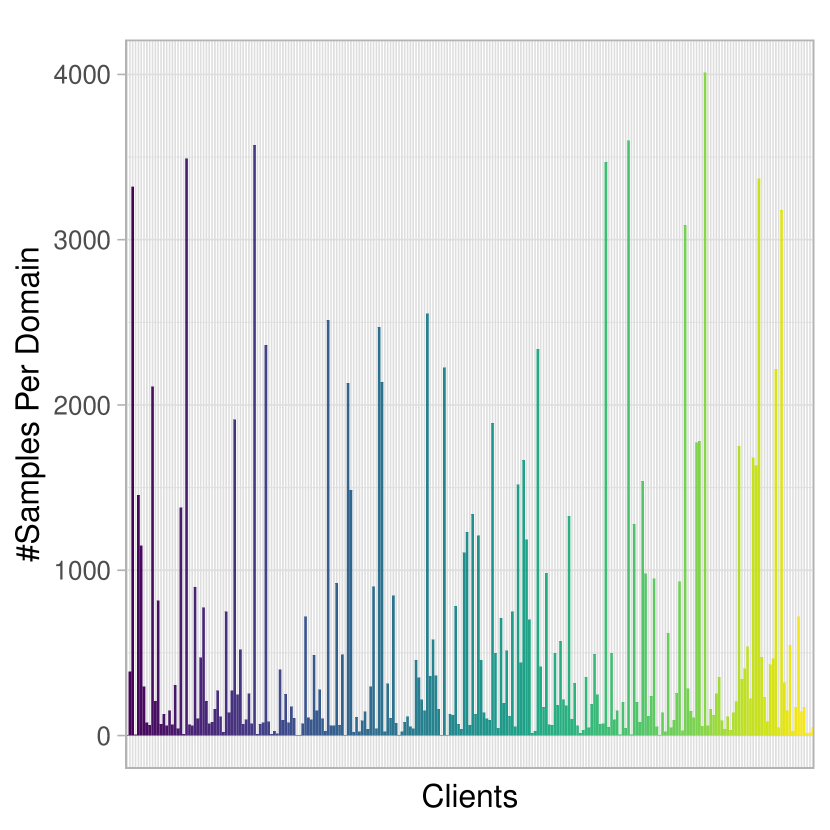
(a) $\lambda=0.0$

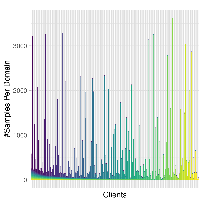
(b) $\lambda=0.1$

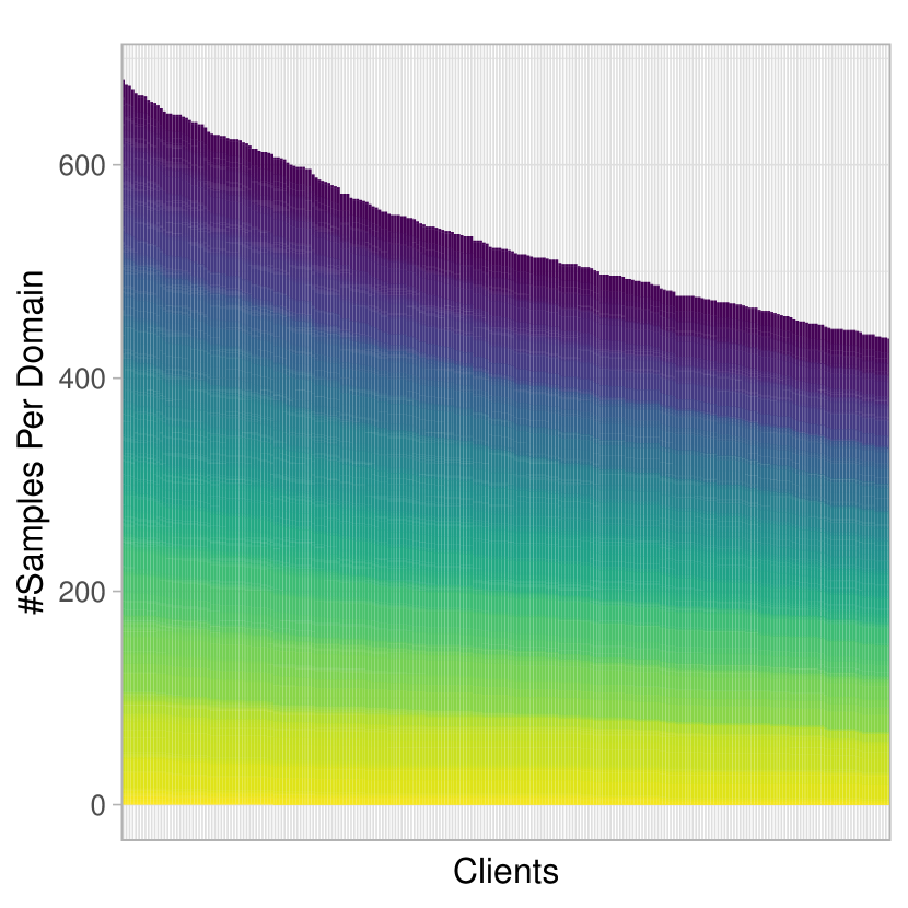
(c) $\lambda=1.0$

Figure 8: Client’s domain heterogeneity distribution with large number of domains (IWildCam)

A.3 Hyper-parameters used with FISC

In this subsection, we present how to select hyper-parameters used within FISC, including Contrastive Loss Coefficient $\lambda_{1}$, Regularization Loss Coefficient $\lambda_{2}$, and Triplet Loss Margin $\alpha$.

A.3.1 Contrastive Loss Coefficient $\gamma_{1}$

This parameter balances the trade-off between learning the main task and the generalization level of each client. The higher this parameter is, the more deviated the local model is toward the global-sharing styled data. However, this may cause a counter-effective result if the style-transferred data does not contain an informative style. Therefore, we suggest to set this parameter no larger than 1.0, i.e., the coefficient for cross-entropy loss. Through empirical grid-searching, we found $\alpha\in[0.5,0.75]$ is the best setting for all three datasets.

Table 5: Comparison of our method and selected baselines

	Local domain signal	Generalization method	Consider non-isolated domain distribution	Consider client sampling	Consider domain-based client heterogeneity
FedSR Nguyen et al. [2022b]	representation’s marginal alignment	local regularization	✗	✗	✗
FedGMA Tenison et al. [2023]	gradient sign	global gradient masking	✗	✗	✗
FedDG-GA Zhang et al. [2023]	training loss difference	weighted averaging	✗	✗	✗
FPL Huang et al. [2023]	class’s prototype	contrastive learning	✓	✗	✗
CCST Chen et al. [2023]	style statistic	training augmented data	✗	✗	✗
Ours	style statistic	contrastive learning	✓	✓	✓

A.3.2 Regularization Loss Coefficient $\gamma_{2}$

Since the deep neural network has more parameters and is easier to overfit, especially when training samples are insufficient, regularization is widely used together with contrastive learning to prevent this Sohn [2016], Tanveer et al. [2021]. When $\beta$ = 0 or negligible, there is no regularization for embedding vectors, which could lead to overfitting, especially when the style transfers are not meaningful. The opposite underfit criterion can happen with a high $\beta$ value. Upon grid searching, this value was observed to give the best performance on $[0.05,0.2]$. For the PACS dataset, we set this value to $0.2$, while the corresponding values for Office-Home and IWildCam are $0.1$ and $0.05$, respectively.

A.3.3 Triplet Loss Margin $\alpha$

The margin parameter specifies the minimum distance that has to be kept between the anchor and the positive example and the maximum distance that has to be retained between both the anchor and the negative example, which is more dependent upon the selection of triplet loss. In our experiments, we set this parameter for PACS and Office-Home to $0.3$, and the corresponding number for IWildCam is $1.0$ since each client in the setting with IWildCam has more samples than the other two datasets. This parameter can be tuned to prevent the vanishing of the triplet loss over each batch and should be set in a $[0.1,1.0]$ range.

A.4 Hyper-parameters used within the baselines

Discussion of baseline selection. We select four SOTA methods corresponding to different approaches mentioned in the Related Work and summarize them as follows:

• FedSR Nguyen et al. [2022b]: Restricting the complexity of the representation can help with the marginal alignment of the representation. Minimizing the representation also helps minimize the distribution distance between the specific and reference domains.

• FedGMA Tenison et al. [2023]: Defining a term called “agreement score” as the percentage of signed agreement (+ or -) among client updates to ensure that global model updates follow their agreement across clients.

• FedDG-GA Zhang et al. [2023]: Defining a term called “flatness” of each domain, which can be presented as a generalization gap between the local and client models (i.e., expected loss difference). Then, adding this term to the global model’s objective function ensures the global model’s flatness on all domains.

• FPL Huang et al. [2023]: Grouping semantically similar prototypes for each class and then averaging them is more efficient than averaging all prototypes to get global prototypes directly. The objective is to handle cases when multiple clients have the same domain. Using contrastive learning to help learn features close to the most representative cluster and separate them from the far-class prototypes.

• CCST Chen et al. [2023]: Generating augmented data via cross-client style transfer (CCST) without exchanging data samples to help create more uniform distributions of source clients and making each local model learn to fit the image styles of all the clients to avoid the different model biases. This method is different from ours since, in this method, style statistics to conduct style transfer are randomly selected from other clients’ styles, while FISC calculates only one interpolation style, which is the aggregate of all client styles. As a result, FISC can help all clients agree on one interpolation style and avoid the randomness of selecting cross-client styles.

We present the conceptual comparison of our method and selected baselines in Table 5. It is worth noting that FISC is the only method considering non-isolated domain distribution, client sampling, and domain-based client heterogeneity simultaneously, addressing the limitation of previous baselines.

A.5 Baselines

FedSR’s Hyper-parameters. In FedSR, there are two parameters which are $\alpha^{L2R},\\ \alpha^{CMI}$, corresponding to two coefficients of the regularization terms in FedSR. Following the original paper, these two parameters are set to $0.01,0.001$, respectively.
FedDG-GA’s Hyper-parameters. The initial step size $d$ belongs to the range of $[0,1]$ for this method, and we set it to $1/3$ as the implementation following the official implementation of FedDG-GA. This step size is decayed by round using $d^{r}=(1-r/R)*d$, where $r$ is the current round and $R$ is the total number of communication rounds. As noted in the original paper, improvement of this method is not sensitive to the specific choices of step size and is consistent with or without the linear decay strategy.
FedGMA’s Hyper-parameters. This work introduces $\tau\in\{0,1\}$, a hyperparameter thresholds agreement across clients. It marks the minimum agreement required to consider the gradient for aggregation. This parameter is set to $0.4$, as suggested by the original paper.
FPL’s Hyper-parameters. In this method, the temperature of the contrastive loss function is controlled by $\tau$. This parameter is set to $0.2$ following the authors’ empirical study.
CCST’s Hyper-parameters. In this method, we set the augmentation level $K$ to 1, where $K$ is the number of styles from style bank B for the augmentation of each image, indicating the diversity of the final augmented data set.

Appendix B Additional Results

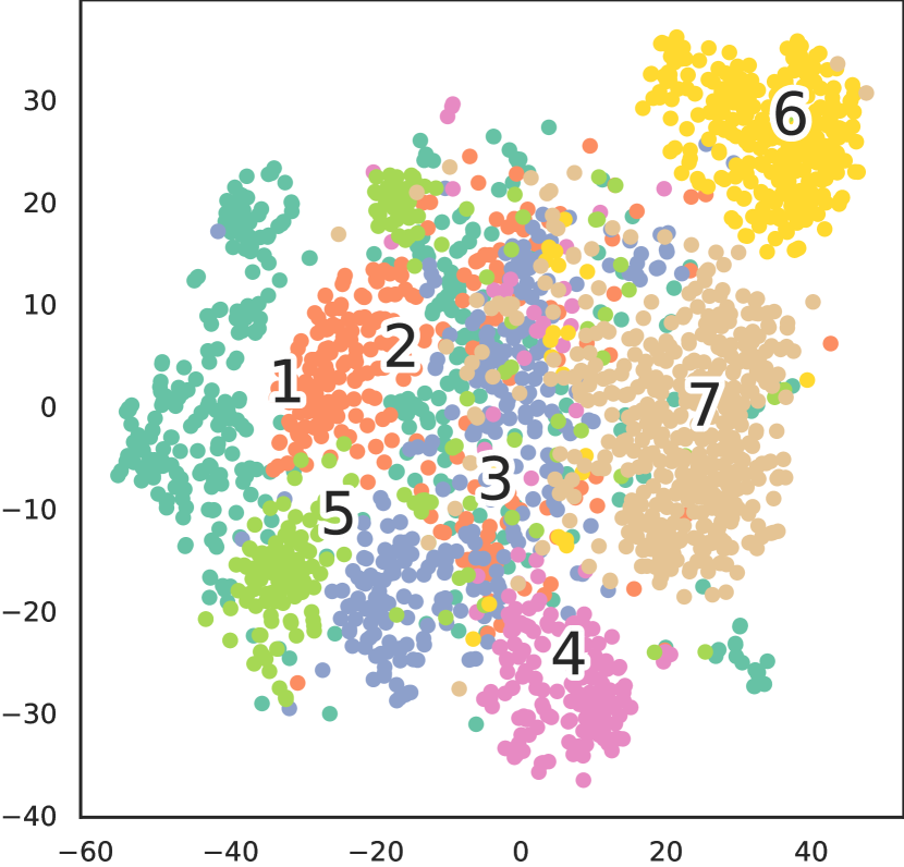
(a) Round 0.

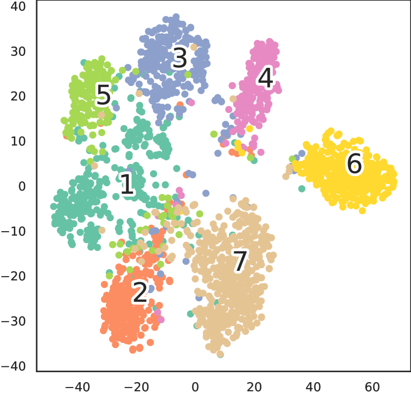
(b) Round 10.

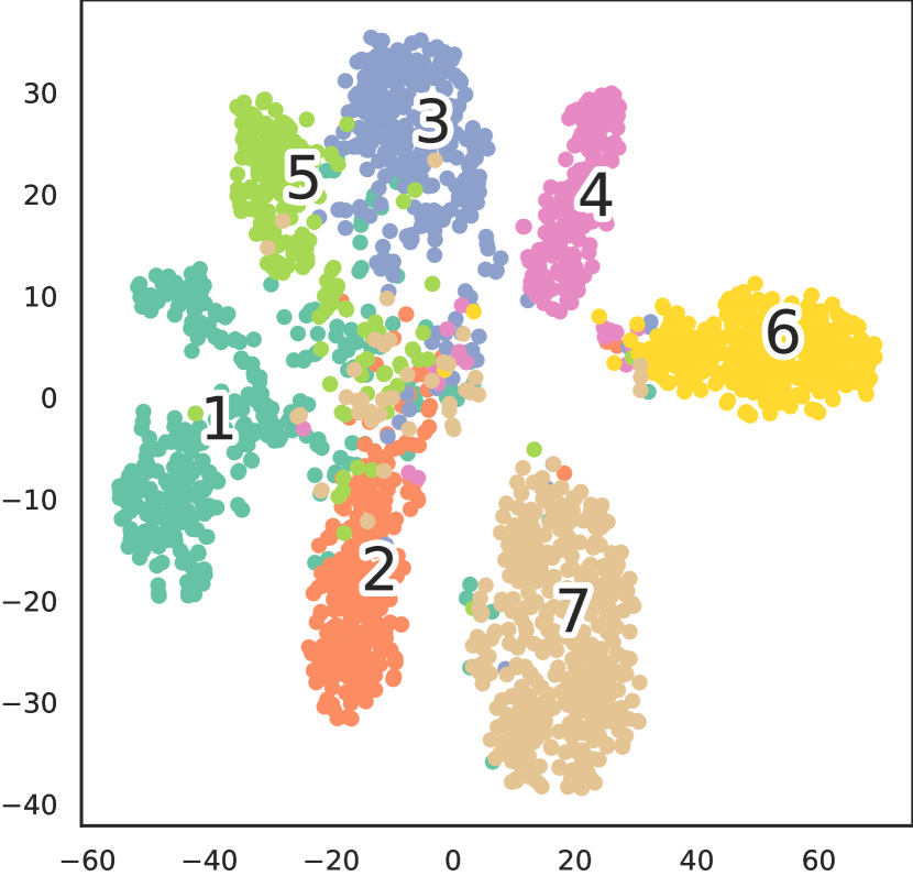
(c) Round 20.

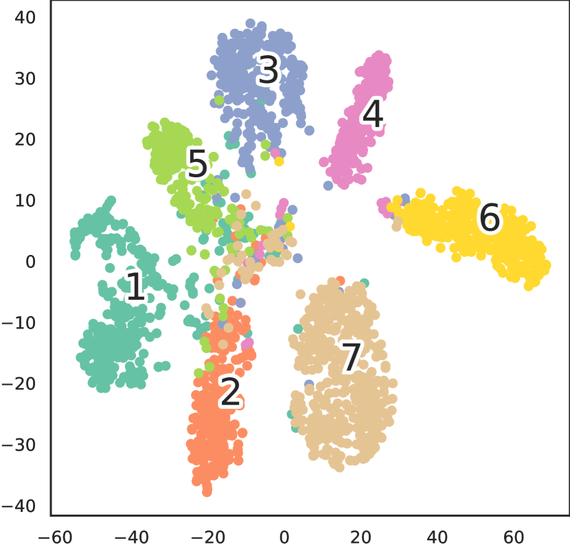
(d) Round 30.

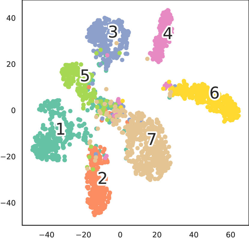
(e) Round 40.

Figure 9: t-SNE Visualization of FISC’s feature extractor at different communication rounds of the global model from PACS. Starting from round 10, the decision boundary among different classes becomes clearer.

We use t-SNE Pedregosa et al. [2011] to visualize FISC’s feature extractor performance by round in Figure. 9. As presented, the feature extractor trained by FISC can discriminate classes clearly after the first 10 training rounds.

Table 6: Accuracy of different methods under different data heterogeneity schemes.

	Methods	$\lambda=0.0$	$\lambda=0.1$	$\lambda=0.5$	$\lambda=1.0$	AVG
Test Accuracy	FedSR	13.34%	13.97%	13.41%	13.21%	13.48%
	FedGMA	59.15%	64.95%	61.59%	51.26%	59.24%
	FedDG-GA	52.46%	63.55%	55.74%	58.16%	54.48%
	FPL	62.13%	56.20%	65.18%	48.99%	58.13%
	CCST	69.41%	63.12%	66.86%	58.23%	64.41%
	Ours	67.01%	66.20%	61.26%	66.20%	65.17%
Validation Accuracy	FedSR	14.96%	14.67%	12.81%	14.01%	14.11%
	FedGMA	94.49%	94.13%	96.23%	92.81%	94.42%
	FedDG-GA	95.93%	92.46%	98.26%	94.25%	95.23%
	FPL	95.51%	94.61%	97.13%	95.57%	95.96%
	CCST	96.05%	96.47%	97.19%	94.64%	96.09%
	Ours	97.72%	95.57%	97.31%	97.13%	96.93%

Then, the detailed results for the Impact of Domain Heterogeneity and the Impact of the Number of Clients are presented in Table 6 and Table 7.

B.1 Impact of Domain Heterogeneity

This experiment aims to study the effectiveness of different methods with different domain distribution settings. In this experiment, the training domains are Art-Painting and Cartoon, and the validation and testing domains are Photo and Sketch from PACS datasets, respectively. We observe the accuracy when varying the domain heterogeneity using $\lambda=\left\{0.0,0.1,0.5,1.0\right\}$ values. As presented in Table 6, FISC outperforms all the baselines with the gap compared to the second-best method is 9%. In conclusion, our method consistently outperforms other baselines under varied domain heterogeneity.

B.2 Impact of the Number of Clients

Table 7: Different FL settings of number of clients

	Settings (K/N)	5/5	5/10	5/50	5/100	5/200	AVG
Validation Accuracy	FedSR	14.45%	14.01%	13.83%	13.62%	13.13%	13.81%
	FedGMA	83.59%	79.59%	42.48%	47.31%	41.70%	58.93%
	FPL	83.74%	80.18%	75.78%	58.64%	50.37%	69.74%
	FedDG-GA	77.49%	75.34%	68.41%	65.28%	52.44%	68.22%
	CCST	82.52%	80.91%	68.26%	66.75%	57.03%	71.09%
	Ours	81.05%	83.69%	79.44%	73.24%	62.16%	75.92%
Test Accuracy	FedSR	13.53%	15.04%	15.19%	13.77%	12.34%	13.97%
	FedGMA	92.93%	91.38%	65.69%	70.78%	71.68%	78.49%
	FPL	93.35%	93.95%	93.77%	83.89%	76.11%	88.21%
	FedDG-GA	86.11%	88.14%	89.46%	87.26%	69.40%	83.67%
	CCST	91.26%	92.57%	85.15%	83.25%	76.23%	85.69%
	Ours	91.44%	93.41%	95.21%	93.23%	77.72%	90.14%

This experiment studies the performance of different baselines under a wide range of clients $N$. We consider five cases: $N\in\{5,10,50,100,200\}$ and $K=5$, which correspond to 100%, 50%, 10%, 5%, and 2.5% clients participating in each round, respectively. In this experiment, the training domains are Sketch and Cartoon, and the validation and testing domains are Photo and Art-Painting from PACS datasets, respectively. As seen in Table 7, our method outperforms in terms of stability and efficiency. We achieve low variance and the highest average accuracy across considered scenarios.

B.3 Effect of Hyper-parameters

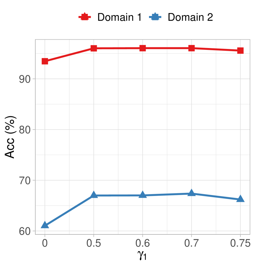
(a) Contrastive Loss Coefficient $\gamma_{1}$.

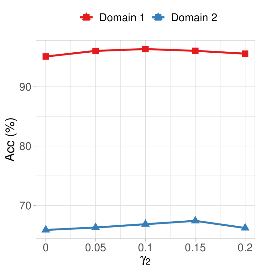
(b) Regularization Loss Coefficient $\gamma_{2}$.

Figure 10: Effect of hyper-parameters on the performance of FISC with PACS dataset.

To assess the stability and effectiveness of the FISC method, we conducted a series of experiments focused on two key parameters, $\gamma_{1}\in\left[0.5,0.75\right]$ and $\gamma_{2}\in\left[0.05,0.2\right]$, which play a critical role in the local contrastive learning component ( Eqn. 7) of our approach. The results in Fig. 10 demonstrate that FISC exhibits stable performance across the suggested ranges for both parameters. For $\gamma_{1}$, the values of P and S remain consistently high, with P showing a slight decrease only at the upper boundary, and S maintaining stable behavior with a peak at $\gamma_{1}=0.7$. Similarly, for $\gamma_{2}$, the performance metrics show minimal fluctuation, with P remaining above 96.0 for most of the range and S reaching its peak at $\gamma_{2}=0.15$. These findings highlight the robustness of FISC, ensuring reliable and consistent performance within these parameter ranges across different scenarios. In this experiment, the training domains are Art-painting and Cartoon, and the validation and testing domains are Photo and Sketch from PACS datasets, respectively.

B.4 Computation Time

Table 8: Computational overhead of different FedDG methods, which is broken down into local training time, aggregation time and one-time cost.

	FedSR	FedGMA	FPL	FedDG-GA	CCST	FISC
Local Training (s)	8.66	7.63	6.29	11.92	9.60	7.94
Aggr. (s)	0.57	1.77	4.31	3.85	0.57	0.57
One-time cost (s)	0	0	0	0	2.89	3.30

For the computation time measurement, we used the same SEED for all experiments and the consistent settings for all baselines, including the number of clients, the local data that each client owns, and the indices of clients selected in each round. Then, for the local training time, we average the training time for all clients in each round for a fair comparison of each baseline. As presented in Table. 8, the average computation time of FISC is comparable to or even smaller than other baselines: (i) FISC does not introduce overhead during aggregation, which is linearly increasing by time as FedDGGA, FedGMA, or FPL. The overhead of avg. local training is comparable to other methods. The cost for interpolation style calculation is a one-time cost, happening before the training and only takes 3.3(s), while the general local training takes 8.67(s) in an average of all methods. This one-time cost does not increase linearly with the number of clients since all clients can conduct local style extraction at the same time, and the clustering at the server is fast (only 0.3s). Since FISC does not modify the aggregation step, this method does not introduce additional overhead to the aggregation phase; which is similar to CCST and FedSR. Regarding the local training time, FISC only needs to use the contrastive loss on the embedding of original batch data and style-transferred batch data. This loss functions are computed on a per-batch basis, which is typical in deep learning training pipelines. Since the batch size $\mathcal{B}$ in Algo. 2 is usually manageable, the additional overhead introduced by the triplet loss and regularizer remains minimal compared to the overall training process. The result in Table. 8 shows that the overall training time and resource consumption remain comparable to models without these components. Other baselines such as FedSR or FedDGGA introduce much overhead in local training because each client needs to maintain an additional probabilistic representation network for distribution sampling (FedSR) or inference on the training data to submit the training loss difference (FedDGGA). To this end, FISC does not introduce difficulty when applied to large-scale systems.

B.5 Security Analysis

Table 9: Comparison metrics for quality of reconstructed images from generative models with MSE and LPIPS losses.

Metrics		P	A	C	S
Inception Score	Real Images	10.3744 $\pm$ 0.6525	10.1615 $\pm$ 1.159	4.764 $\pm$ 0.2522	2.52 $\pm$ 0.0758
	Style2Image - MSE	0.1828 $\pm$ 0.00047	0.1763 $\pm$ 0.0005	0.216 $\pm$ 0.00067	0.2183 $\pm$ 0.00023
	Style2Image - LPIPS	0.273 $\pm$ 0.0008	0.289 $\pm$ 0.0005	0.257 $\pm$ 0.0007	0.2256 $\pm$ 0.0012
FID	Baseline-GAN	59.185	126.72	118.66	321.59
	Style2Image - MSE	365.873	415.45	343.66	360.365
	Style2Image - LPIPS	342.12	379.03	310.53	362.56

Table 10: The performance of FISC on PACS dataset after incorporating privacy-preserving techniques. $s$ represents the scale parameter for the noise distribution generation and $p\in(0,1)$ represents the perturbation coefficient of the noise.

Methods	Test Domain
	P	S	A	C	AVG
$p=0.1,s=0.02$	90.84	66.94	73.49	51.96	70.81
$p=0.1,s=0.05$	89.70	67.12	73.88	48.93	69.91
Original	93.05	66.20	71.73	53.11	71.02

Firstly, we argue that our method is more effective in avoiding inter-client inference attacks compared to the cross-client sharing mechanism discussed in the Security Analysis section of the main paper. This is primarily because our method relies on using images transferred from the interpolation style, which do not contain domain-specific characteristics. By omitting these domain-specific features, the transferred images are significantly different from the real images, making it more challenging for an attacker to infer sensitive information. This approach enhances the security of client data in federated learning scenarios by reducing the risk of inter-client inference attacks.

Second, we conducted experiments to evaluate the vulnerability of our method to third-party or server-side reconstruction attacks, specifically focusing on the scenario where an external attacker, pre-trained on large-scale images, compromises the style vectors and attempts to reconstruct the original images. To simulate this attack, we trained a generator using a state-of-the-art GAN[1] on the Tiny-ImageNet[2] dataset, employing both Mean Squared Error (MSE) and Learned Perceptual Image Patch Similarity (LPIPS) losses to guide the reconstruction process from the shared style vectors. For comparison, the baseline model was trained on real images, representing an ideal yet impractical scenario where the attacker has direct access to client data. The results in Table. 9 indicate that the images reconstructed from the style vectors are vastly different from the original images, as well as from the images generated by the baseline GAN model. This is evidenced by significant differences in key evaluation metrics, such as the Inception Score (IS) and the Fréchet Inception Distance (FID). Specifically, the reconstructed images from the style vectors achieved substantially lower IS values and higher FID scores compared to real images and the baseline, underscoring the poor quality and substantial divergence of these reconstructions. For instance, while the IS for real images was above 10 for datasets P and A, the Style2Image reconstructions yielded IS scores below 0.3, and the FID scores for these reconstructions were several times higher than those of the baseline model. These findings strongly suggest that reconstructing a client’s data using only the style vectors in our approach is highly non-trivial, making it difficult for an attacker to derive meaningful or accurate representations of the original images. Therefore, our method effectively mitigates the risk of data reconstruction attacks, further enhancing the security and privacy of client data in federated learning environments.

Third, the practice of sharing class-wise mean values of embedding vectors during training has gained traction in federated learning, as seen in recent works such as FedDG and others Tan et al. [2022], Zhang et al. [2024], Huang et al. [2023], Liu et al. [2021a]. However, compared to these approaches, FISC offers superior privacy-preserving capabilities by avoiding sharing any class-level information. Instead, FISC only transmits channel-wise embedding vector statistics once before training begins, reducing the exposure of sensitive data. This limited sharing significantly lowers the risk of privacy breaches and makes it more challenging for adversaries to infer class-specific information. Moreover, FISC facilitates the integration of additional privacy-preserving techniques, such as adding noise to the local style during the initialization phase, without compromising performance. In line with the setups of FedPCL Tan et al. [2022] and DBE Zhang et al. [2024], we experimented with adding Gaussian noise to the client style using controllable parameters like the noise scale ($s$) and perturbation coefficient ($p$). The results indicate that introducing perturbations does not lead to a significant drop in accuracy but effectively enhances privacy protection. For instance, the average accuracy across domains remains competitive, with minor differences when applied perturbation, as shown in Table. 10. Specifically, the model’s performance with $p=0.1$ and $s=0.02$ achieves an average accuracy of 70.81%, closely matching the original accuracy of 71.02%, demonstrating the robustness of FISC in maintaining utility even under privacy-preserving transformations. In summary, reconstructing local data using client-style statistics in our approach is notably challenging, and adding mechanisms like Gaussian noise at the client level before transmitting the style to the server provides additional protection without degrading utility. FISC achieves state-of-the-art performance while upholding stringent privacy-preserving mechanisms, ensuring that privacy and performance are not mutually exclusive.

B.6 Ablation Study

Table 11: Performance of FISC with different components present – removed components (✗) / retained (✓).

Methods	Components			Performance
	Local Clustering	Global Clustering	Contrastive Learning	Validation Accuracy	Test Accuracy
FISC-v1	✗	✓	✓	72.90%	92.22%
FISC-v2	✓	✗	✓	72.80%	92.18%
FISC-v3	✓	✓	✗	64.89%	85.69%
FISC-v4	✗	✗	✓	59.42%	82.33%
FISC-v5	✓	✓	✓	73.63%	93.05%

In Table 11, we conduct an ablation study to investigate the impacts of the main components proposed in our FISC approach. We gradually remove each component from FISC architecture to construct four incomplete versions of FISC. In the FISC-v1 and FISC-v2 versions, the ✗ cells indicate that simple averaging was used to calculate the local and global styles, rather than the clustering methods described earlier. The results demonstrate that clustering at both the local and global levels is essential in mitigating the bias introduced by domain heterogeneity, proving to be more effective than simple averaging. The performance limitations of the simple averaging approach underscore the necessity for clustering, with FINCH outperforming simple averaging in both versions. The contrastive learning component in FISC-v3 is identified as the second-most critical element. Excluding this component leads to a significant 9% drop in accuracy, even when style-transferred data is added to the training. This result underscores the importance of the carefully designed combination of interpolation style and contrastive learning. However, it is important to note that the effectiveness of the contrastive learning component hinges on the use of interpolation style-transferred data. This is evident from the comparison between FISC-v4 and FISC-v5, where FISC-v4—relying on standard contrastive learning with augmentation and close samples as positive anchors—fails to address domain shifts effectively in federated learning, unlike FISC-v5, which utilizes interpolation style-transferred data. In conclusion, the FISC-v5 version, which incorporates all components, demonstrates superior performance in handling unseen domain accuracy, reinforcing the value of the well-designed components of FISC.

Appendix C Limitations

The main limitation of this work is the intuition of style definition. We use the style as the statistic of the embedding vector, which is every channel’s mean and standard deviation. The style-transfer models are often pre-trained on large datasets of color images, such as ImageNet Huang and Belongie [2017], which contain a vast array of color variations, textures, and patterns. As a result, the learned representations inherently capture the color information. As a result, we hypothesize that our method will not perform well with gray-scaled datasets. Taking the FEMNIST Caldas et al. [2018] dataset as an example, the style of each image relies heavily on the content itself, i.e., the hand-written style of each individual. Other than that, backgrounds in other pixels do not help determine the style of these images.

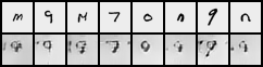
Figure 11: FEMNIST’s style-transferring data. The first row is the original images, and the second is the corresponding style-transferred images.

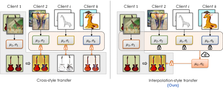
Figure 12: Other cross-transfer methods and ours.

We illustrate the images generated by FISC with the FEMNIST dataset in Figure. 11. Using the current style of statistical information and interpolative style extraction method Figure. 12 despite preserving information ability may introduce noise or distortion to the original images, leading to degradation in model accuracy.

One of the potential solutions for this is to change the style extraction component specialized for learning tasks — datasets, e.g., hand-written images Kang et al. [2021], Fu et al. [2022] and gray-scaled images Liu et al. [2021b]. We will address this in future works.

Appendix D Societal Impacts

Our method (FISC) aims to improve existing FedDG approaches by addressing the challenge of domain shift in Federated Learning (FL). We focus on domain-based client heterogeneity and client sampling to enhance the generalizability of FL schemes across multiple domains while preserving privacy. By centralizing local style statistics on the server and using contrastive learning techniques, FISC helps protect privacy while enabling the sharing of interpolative styles from multiple clients across distributed clients. This approach ensures individuals’ data privacy and fosters trust in data-driven applications across different domains. This method supports AI learning in real-world applications where addressing domain shift while preserving privacy is essential for deploying AI solutions effectively and ethically, such as healthcare, smart cities, social media, etc. In addition, FISC’s effectiveness in handling domain shift promotes fairness in AI systems, ensuring models perform well across diverse domains and demographic groups, thus reducing the risk of biased outcomes. This contributes to building more inclusive AI technologies. In broader impact, FISC can accelerate progress in machine learning research and address complex societal challenges such as healthcare disparities, environmental sustainability, and social equity. By ensuring privacy protection, promoting equity, facilitating collaboration, and supporting responsible data use, FISC contributes to a more responsible and trustworthy AI ecosystem, benefiting individuals, organizations, and society.

Appendix E Pseudo Algorithms

The detailed pseudo algorithm for FISC is presented in Algorithm 1 and Algorithm 2.

Algorithm 1 FISC

1:Input:

2:$G_{0}$: Initial global model

3:$T$: Total training rounds

4:$N$: Total clients

5:$K$: Total participating clients per training round

6:$n_{i},\forall i\in N$: Size of local training data

7:Output: $G^{T}$: Updated global model after $T$ training iterations

8:for client $\mathcal{C}_{i}\ \forall i\in[1,\ldots,N]$ do

9:     $\Phi(\mathcal{C}_{i})\leftarrow\{\Phi(x_{j})\mid\forall x_{j}\in\mathcal{D}_{i}\}$ $\triangleright$ Local data of client $i$

10:     $\Phi(\mathcal{C}_{k})\xrightarrow{\text{ FINCH }}\Gamma_{L_{k}}=\left\{\Phi_{j}\right\}_{j=1}^{L_{k}}\in\mathbb{R}^{L_{k}\times d\times w\times h}$

11:     $\mathcal{S}(\Phi_{j})\leftarrow\left(\mu\left(\Phi_{j}\right),\sigma\left(\Phi_{j}\right)\right)\in\mathbb{R}^{2d}$

12:     $S_{\mathcal{C}_{k}}\leftarrow\frac{1}{L_{k}}\sum_{i=1}^{L_{k}}\mathcal{S}(\Phi_{i})\in\mathbb{R}^{2d}$

13:end for

14:Server collects local style from $N$ clients and conducts interpolation style extraction

15:$\mathbf{S}=\left\{\mathcal{S}_{\mathcal{C}_{i}}\right\}_{i=1}^{N}\xrightarrow{\text{ FINCH }}\Gamma_{L}=\left\{\mathcal{S}_{j}\right\}_{j=1}^{L}\in\mathbb{R}^{L\times 2d}$

16:$\mathcal{S}_{g}\leftarrow\text{median}\left(S_{j}\mid\forall S_{j}\in\Gamma_{L}\right)\in\mathbb{R}^{2d}$ $\triangleright$ Interpolative style

17:for iteration $t$ in $[1,\ldots,T]$ do

18:     Server samples a subset $\mathcal{C}=\{\mathcal{C}_{1},\mathcal{C}_{2},\ldots,\mathcal{C}_{i},\ldots,\mathcal{C}_{K}\}$ of $K$ clients randomly from $N$ clients;

19:     for each client $i$ in $\mathcal{C}_{t}$ do

20:         $G^{t}_{i}\leftarrow\text{ContrastiveTraining}(G_{t-1})$

21:     end for

22:     $G_{t}\leftarrow\frac{1}{N}\sum_{i=1}^{K}n_{i}G_{i}^{t}$ $\triangleright$ with $N=\sum_{i=1}^{K}n_{i}$

23:end for

24:return $G_{T}$

Algorithm 2 ContrastiveTraining

1:Input:

2:$G_{t-1}$: Global model at previous round

3:$\mathcal{S}_{g}$: Interpolative style

4:$\mathcal{D}_{i}$: Local training data of the $i$-th client

5:Output: $G^{i}_{t}$: Updated global model at $t$-th communication round.

6:Initialize $G^{i}_{t}\leftarrow G_{t-1}$;

7:for each batch $\mathcal{B}$ in $\mathcal{D}_{i}$ do

8:     $\mathcal{B}_{p}\leftarrow\{\text{AdaIN}(z_{i},\mathcal{S}_{g}),y_{i}\mid\forall z_{i}\in\mathcal{B}\}$ $\triangleright$ Generate style-transferred data $\mathcal{B}_{p}$

9:     Sample triplets $\{\textbf{z}^{a},\textbf{z}^{p},\textbf{z}^{n}\}$ for this batch;

10:     $\mathcal{L}_{T}\leftarrow\frac{1}{|\mathcal{B}|}\sum_{i=1}^{|\mathcal{B}|}\left[\left\|z_{i}^{a}-z_{i}^{p}\right\|_{2}^{2}-\left\|z_{i}^{a}-z_{i}^{n}\right\|_{2}^{2}+\alpha\right]$;

11:     $\mathcal{L}_{reg}\leftarrow\frac{1}{|\mathcal{B}|}\sum_{i=1}^{|\mathcal{B}|}\left(\left(z_{i}^{a}\right)^{2}+\left(z_{i}^{p}\right)^{2}\right)$;

12:     $\mathcal{L}_{CE}\leftarrow-\frac{1}{|\mathcal{B}|}\sum_{i=1}^{|\mathcal{B}|}\mathbf{1}_{y_{i}}\log\left(\text{softmax}\left(g\left(z_{i}\right)\right)\right)$;

13:     $\mathcal{L}\leftarrow\mathcal{L}_{CE}+\alpha\mathcal{L}_{T}+\beta\mathcal{L}_{reg}$;

14:     $G_{i}^{t}\leftarrow G_{i}^{t}-\eta\nabla\mathcal{L}\left(G_{i}^{t}\right)$

15:end for

16:return $G^{t}_{i}$

References

- McMahan et al. [2017] Brendan McMahan, Eider Moore, Daniel Ramage, Seth Hampson, and Blaise Aguera y Arcas. Communication-efficient learning of deep networks from decentralized data. In Artificial intelligence and statistics, pages 1273–1282. PMLR, 2017.
- Sheller et al. [2020] Micah J Sheller, Brandon Edwards, G Anthony Reina, Jason Martin, Sarthak Pati, Aikaterini Kotrotsou, Mikhail Milchenko, Weilin Xu, Daniel Marcus, Rivka R Colen, et al. Federated learning in medicine: facilitating multi-institutional collaborations without sharing patient data. Scientific reports, 10(1):12598, 2020.
- Nguyen et al. [2021a] Dinh C Nguyen, Ming Ding, Pubudu N Pathirana, Aruna Seneviratne, Jun Li, and H Vincent Poor. Federated learning for internet of things: A comprehensive survey. IEEE Communications Surveys & Tutorials, 23(3):1622–1658, 2021a.
- Li et al. [2020] Tian Li, Anit Kumar Sahu, Manzil Zaheer, Maziar Sanjabi, Ameet Talwalkar, and Virginia Smith. Federated optimization in heterogeneous networks. Proceedings of Machine learning and systems, 2:429–450, 2020.
- Karimireddy et al. [2020] Sai Praneeth Karimireddy, Satyen Kale, Mehryar Mohri, Sashank Reddi, Sebastian Stich, and Ananda Theertha Suresh. Scaffold: Stochastic controlled averaging for federated learning. In International conference on machine learning, pages 5132–5143. PMLR, 2020.
- Mendieta et al. [2022] Matias Mendieta, Taojiannan Yang, Pu Wang, Minwoo Lee, Zhengming Ding, and Chen Chen. Local learning matters: Rethinking data heterogeneity in federated learning. In Proceedings of the IEEE/CVF Conference on Computer Vision and Pattern Recognition, pages 8397–8406, 2022.
- Lim et al. [2024] Jin Hyuk Lim, SeungBum Ha, and Sung Whan Yoon. Metavers: Meta-learned versatile representations for personalized federated learning. In Proceedings of the IEEE/CVF Winter Conference on Applications of Computer Vision, pages 2587–2596, 2024.
- Wang et al. [2020] Hongyi Wang, Mikhail Yurochkin, Yuekai Sun, Dimitris Papailiopoulos, and Yasaman Khazaeni. Federated learning with matched averaging. In International Conference on Learning Representations, 2020. URL https://openreview.net/forum?id=BkluqlSFDS.
- Gao et al. [2022] L Gao, H Fu, L Li, Y Chen, M Xu, and C-Z Feddc Xu. Federated learning with non-iid data via local drift decoupling and correction. In Proceedings of the IEEE/CVF Conference on Computer Vision and Pattern Recognition, New Orleans, LA, USA, pages 18–24, 2022.
- Li et al. [2021] Qinbin Li, Bingsheng He, and Dawn Song. Model-contrastive federated learning. In Proceedings of the IEEE/CVF conference on computer vision and pattern recognition, pages 10713–10722, 2021.
- Nguyen et al. [2022a] Nang Hung Nguyen, Phi Le Nguyen, Thuy Dung Nguyen, Trung Thanh Nguyen, Duc Long Nguyen, Thanh Hung Nguyen, Huy Hieu Pham, and Thao Nguyen Truong. Feddrl: Deep reinforcement learning-based adaptive aggregation for non-iid data in federated learning. In Proceedings of the 51st International Conference on Parallel Processing, pages 1–11, 2022a.
- Orlando et al. [2020] José Ignacio Orlando, Huazhu Fu, João Barbosa Breda, Karel Van Keer, Deepti R Bathula, Andrés Diaz-Pinto, Ruogu Fang, Pheng-Ann Heng, Jeyoung Kim, JoonHo Lee, et al. Refuge challenge: A unified framework for evaluating automated methods for glaucoma assessment from fundus photographs. Medical image analysis, 59:101570, 2020.
- Guo et al. [2023] Jintao Guo, Lei Qi, and Yinghuan Shi. Domaindrop: Suppressing domain-sensitive channels for domain generalization. In Proceedings of the IEEE/CVF International Conference on Computer Vision, pages 19114–19124, 2023.
- Huang et al. [2023] Wenke Huang, Mang Ye, Zekun Shi, He Li, and Bo Du. Rethinking federated learning with domain shift: A prototype view. In 2023 IEEE/CVF Conference on Computer Vision and Pattern Recognition (CVPR), pages 16312–16322. IEEE, 2023.
- Sun and Saenko [2016] Baochen Sun and Kate Saenko. Deep coral: Correlation alignment for deep domain adaptation. In Computer Vision–ECCV 2016 Workshops: Amsterdam, The Netherlands, October 8-10 and 15-16, 2016, Proceedings, Part III 14, pages 443–450. Springer, 2016.
- Nguyen et al. [2021b] A Tuan Nguyen, Toan Tran, Yarin Gal, and Atilim Gunes Baydin. Domain invariant representation learning with domain density transformations. Advances in Neural Information Processing Systems, 34:5264–5275, 2021b.
- Wang et al. [2021] Jing Wang, Jiahong Chen, Jianzhe Lin, Leonid Sigal, and Clarence W de Silva. Discriminative feature alignment: Improving transferability of unsupervised domain adaptation by gaussian-guided latent alignment. Pattern Recognition, 116:107943, 2021.
- Li et al. [2018] Da Li, Yongxin Yang, Yi-Zhe Song, and Timothy Hospedales. Learning to generalize: Meta-learning for domain generalization. In Proceedings of the AAAI conference on artificial intelligence, volume 32, 2018.
- Liu et al. [2021a] Quande Liu, Cheng Chen, Jing Qin, Qi Dou, and Pheng-Ann Heng. Feddg: Federated domain generalization on medical image segmentation via episodic learning in continuous frequency space. In Proceedings of the IEEE/CVF Conference on Computer Vision and Pattern Recognition, pages 1013–1023, 2021a.
- Nguyen et al. [2022b] A Tuan Nguyen, Philip Torr, and Ser Nam Lim. Fedsr: A simple and effective domain generalization method for federated learning. Advances in Neural Information Processing Systems, 35:38831–38843, 2022b.
- Tenison et al. [2023] Irene Tenison, Sai Aravind Sreeramadas, Vaikkunth Mugunthan, Edouard Oyallon, Irina Rish, and Eugene Belilovsky. Gradient masked averaging for federated learning. Transactions on Machine Learning Research, 2023. ISSN 2835-8856. URL https://openreview.net/forum?id=REAyrhRYAo.
- Zhang et al. [2023] Ruipeng Zhang, Qinwei Xu, Jiangchao Yao, Ya Zhang, Qi Tian, and Yanfeng Wang. Federated domain generalization with generalization adjustment. In Proceedings of the IEEE/CVF Conference on Computer Vision and Pattern Recognition, pages 3954–3963, 2023.
- Bai et al. [2024] Ruqi Bai, Saurabh Bagchi, and David I. Inouye. Benchmarking algorithms for federated domain generalization. In The Twelfth International Conference on Learning Representations, 2024. URL https://openreview.net/forum?id=wprSv7ichW.
- Fu et al. [2023] Lei Fu, Huanle Zhang, Ge Gao, Mi Zhang, and Xin Liu. Client selection in federated learning: Principles, challenges, and opportunities. IEEE Internet of Things Journal, 2023.
- Crawshaw et al. [2024] Michael Crawshaw, Yajie Bao, and Mingrui Liu. Federated learning with client subsampling, data heterogeneity, and unbounded smoothness: A new algorithm and lower bounds. Advances in Neural Information Processing Systems, 36, 2024.
- Wang et al. [2022] Jindong Wang, Cuiling Lan, Chang Liu, Yidong Ouyang, Tao Qin, Wang Lu, Yiqiang Chen, Wenjun Zeng, and Philip Yu. Generalizing to unseen domains: A survey on domain generalization. IEEE Transactions on Knowledge and Data Engineering, 2022.
- Bai et al. [2023] Ruqi Bai, Saurabh Bagchi, and David I Inouye. Benchmarking algorithms for federated domain generalization. arXiv preprint arXiv:2307.04942, 2023.
- Chen et al. [2023] Junming Chen, Meirui Jiang, Qi Dou, and Qifeng Chen. Federated domain generalization for image recognition via cross-client style transfer. In Proceedings of the IEEE/CVF Winter Conference on Applications of Computer Vision, pages 361–370, 2023.
- Huang and Belongie [2017] Xun Huang and Serge Belongie. Arbitrary style transfer in real-time with adaptive instance normalization. In Proceedings of the IEEE international conference on computer vision, pages 1501–1510, 2017.
- Sarfraz et al. [2019] Saquib Sarfraz, Vivek Sharma, and Rainer Stiefelhagen. Efficient parameter-free clustering using first neighbor relations. In Proceedings of the IEEE/CVF conference on computer vision and pattern recognition, pages 8934–8943, 2019.
- Schroff et al. [2015] Florian Schroff, Dmitry Kalenichenko, and James Philbin. Facenet: A unified embedding for face recognition and clustering. In Proceedings of the IEEE conference on computer vision and pattern recognition, pages 815–823, 2015.
- De Boer et al. [2005] Pieter-Tjerk De Boer, Dirk P Kroese, Shie Mannor, and Reuven Y Rubinstein. A tutorial on the cross-entropy method. Annals of operations research, 134:19–67, 2005.
- Imambi et al. [2021] Sagar Imambi, Kolla Bhanu Prakash, and GR Kanagachidambaresan. Pytorch. Programming with TensorFlow: Solution for Edge Computing Applications, pages 87–104, 2021.
- Li et al. [2017] Da Li, Yongxin Yang, Yi-Zhe Song, and Timothy M Hospedales. Deeper, broader and artier domain generalization. In Proceedings of the IEEE international conference on computer vision, pages 5542–5550, 2017.
- Venkateswara et al. [2017] Hemanth Venkateswara, Jose Eusebio, Shayok Chakraborty, and Sethuraman Panchanathan. Deep hashing network for unsupervised domain adaptation. In Proceedings of the IEEE conference on computer vision and pattern recognition, pages 5018–5027, 2017.
- Koh et al. [2021] Pang Wei Koh, Shiori Sagawa, Henrik Marklund, Sang Michael Xie, Marvin Zhang, Akshay Balsubramani, Weihua Hu, Michihiro Yasunaga, Richard Lanas Phillips, Irena Gao, et al. Wilds: A benchmark of in-the-wild distribution shifts. In International Conference on Machine Learning, pages 5637–5664. PMLR, 2021.
- Liu et al. [2020] Bingchen Liu, Yizhe Zhu, Kunpeng Song, and Ahmed Elgammal. Towards faster and stabilized gan training for high-fidelity few-shot image synthesis. In International conference on learning representations, 2020.
- Heusel et al. [2017] Martin Heusel, Hubert Ramsauer, Thomas Unterthiner, Bernhard Nessler, and Sepp Hochreiter. Gans trained by a two time-scale update rule converge to a local nash equilibrium. Advances in neural information processing systems, 30, 2017.
- Seitzer [2020] Maximilian Seitzer. pytorch-fid: FID Score for PyTorch. https://github.com/mseitzer/pytorch-fid, August 2020. Version 0.3.0.
- Shankar et al. [2018] Shiv Shankar, Vihari Piratla, Soumen Chakrabarti, Siddhartha Chaudhuri, Preethi Jyothi, and Sunita Sarawagi. Generalizing across domains via cross-gradient training. arXiv preprint arXiv:1804.10745, 2018.
- Zhou et al. [2021] Kaiyang Zhou, Yongxin Yang, Yu Qiao, and Tao Xiang. Domain generalization with mixstyle. In International Conference on Learning Representations, 2021. URL https://openreview.net/forum?id=6xHJ37MVxxp.
- Mitrovic et al. [2021] Jovana Mitrovic, Brian McWilliams, Jacob C Walker, Lars Holger Buesing, and Charles Blundell. Representation learning via invariant causal mechanisms. In International Conference on Learning Representations, 2021. URL https://openreview.net/forum?id=9p2ekP904Rs.
- Niu et al. [2023] Ziwei Niu, Junkun Yuan, Xu Ma, Yingying Xu, Jing Liu, Yen-Wei Chen, Ruofeng Tong, and Lanfen Lin. Knowledge distillation-based domain-invariant representation learning for domain generalization. IEEE Transactions on Multimedia, 2023.
- Zhang et al. [2022] Lin Zhang, Li Shen, Liang Ding, Dacheng Tao, and Ling-Yu Duan. Fine-tuning global model via data-free knowledge distillation for non-iid federated learning. In Proceedings of the IEEE/CVF conference on computer vision and pattern recognition, pages 10174–10183, 2022.
- Shi et al. [2022] Yuge Shi, Jeffrey Seely, Philip Torr, Siddharth N, Awni Hannun, Nicolas Usunier, and Gabriel Synnaeve. Gradient matching for domain generalization. In International Conference on Learning Representations, 2022. URL https://openreview.net/forum?id=vDwBW49HmO.
- Arjovsky et al. [2019] Martin Arjovsky, Léon Bottou, Ishaan Gulrajani, and David Lopez-Paz. Invariant risk minimization. arXiv preprint arXiv:1907.02893, 2019.
- Piratla et al. [2020] Vihari Piratla, Praneeth Netrapalli, and Sunita Sarawagi. Efficient domain generalization via common-specific low-rank decomposition. In International Conference on Machine Learning, pages 7728–7738. PMLR, 2020.
- Xu et al. [2021] Qinwei Xu, Ruipeng Zhang, Ya Zhang, Yanfeng Wang, and Qi Tian. A fourier-based framework for domain generalization. In Proceedings of the IEEE/CVF Conference on Computer Vision and Pattern Recognition, pages 14383–14392, 2021.
- Carlucci et al. [2019] Fabio M Carlucci, Antonio D’Innocente, Silvia Bucci, Barbara Caputo, and Tatiana Tommasi. Domain generalization by solving jigsaw puzzles. In Proceedings of the IEEE/CVF Conference on Computer Vision and Pattern Recognition, pages 2229–2238, 2019.
- Hanzely et al. [2020] Filip Hanzely, Slavomír Hanzely, Samuel Horváth, and Peter Richtárik. Lower bounds and optimal algorithms for personalized federated learning. Advances in Neural Information Processing Systems, 33:2304–2315, 2020.
- Qu et al. [2022] Liangqiong Qu, Yuyin Zhou, Paul Pu Liang, Yingda Xia, Feifei Wang, Ehsan Adeli, Li Fei-Fei, and Daniel Rubin. Rethinking architecture design for tackling data heterogeneity in federated learning. In Proceedings of the IEEE/CVF Conference on Computer Vision and Pattern Recognition, pages 10061–10071, 2022.
- Shenaj et al. [2023] Donald Shenaj, Eros Fanì, Marco Toldo, Debora Caldarola, Antonio Tavera, Umberto Michieli, Marco Ciccone, Pietro Zanuttigh, and Barbara Caputo. Learning across domains and devices: Style-driven source-free domain adaptation in clustered federated learning. In Proceedings of the IEEE/CVF winter conference on applications of computer vision, pages 444–454, 2023.
- He et al. [2016] Kaiming He, Xiangyu Zhang, Shaoqing Ren, and Jian Sun. Deep residual learning for image recognition. In Proceedings of the IEEE conference on computer vision and pattern recognition, pages 770–778, 2016.
- Sohn [2016] Kihyuk Sohn. Improved deep metric learning with multi-class n-pair loss objective. Advances in neural information processing systems, 29, 2016.
- Tanveer et al. [2021] Muhammad Tanveer, Hung-Khoon Tan, Hui-Fuang Ng, Maylor Karhang Leung, and Joon Huang Chuah. Regularization of deep neural network with batch contrastive loss. IEEE Access, 9:124409–124418, 2021.
- Pedregosa et al. [2011] F. Pedregosa, G. Varoquaux, A. Gramfort, V. Michel, B. Thirion, O. Grisel, M. Blondel, P. Prettenhofer, R. Weiss, V. Dubourg, J. Vanderplas, A. Passos, D. Cournapeau, M. Brucher, M. Perrot, and E. Duchesnay. Scikit-learn: Machine learning in Python. Journal of Machine Learning Research, 12:2825–2830, 2011.
- Tan et al. [2022] Yue Tan, Guodong Long, Jie Ma, Lu Liu, Tianyi Zhou, and Jing Jiang. Federated learning from pre-trained models: A contrastive learning approach. Advances in neural information processing systems, 35:19332–19344, 2022.
- Zhang et al. [2024] Jianqing Zhang, Yang Hua, Jian Cao, Hao Wang, Tao Song, Zhengui Xue, Ruhui Ma, and Haibing Guan. Eliminating domain bias for federated learning in representation space. Advances in Neural Information Processing Systems, 36, 2024.
- Caldas et al. [2018] Sebastian Caldas, Sai Meher Karthik Duddu, Peter Wu, Tian Li, Jakub Konečnỳ, H Brendan McMahan, Virginia Smith, and Ameet Talwalkar. Leaf: A benchmark for federated settings. arXiv preprint arXiv:1812.01097, 2018.
- Kang et al. [2021] Lei Kang, Pau Riba, Marcal Rusinol, Alicia Fornes, and Mauricio Villegas. Content and style aware generation of text-line images for handwriting recognition. IEEE Transactions on Pattern Analysis and Machine Intelligence, 44(12):8846–8860, 2021.
- Fu et al. [2022] Tsu-Jui Fu, Xin Eric Wang, and William Yang Wang. Language-driven artistic style transfer. In European Conference on Computer Vision, pages 717–734. Springer, 2022.
- Liu et al. [2021b] Kunlin Liu, Dongdong Chen, Jing Liao, Weiming Zhang, Hang Zhou, Jie Zhang, Wenbo Zhou, and Nenghai Yu. Jpeg robust invertible grayscale. IEEE Transactions on Visualization and Computer Graphics, 28(12):4403–4417, 2021b.