Abstract

Machine learning models are increasingly used in critical areas such as loan approvals and hiring, yet they often function as black boxes, obscuring their decision-making processes. Transparency is crucial, as individuals need explanations to understand decisions, primarily if the decisions result in an undesired outcome. Our work introduces CoGS (Counterfactual Generation with s(CASP)), a model-agnostic framework capable of generating counterfactual explanations for classification models. CoGS leverages the goal-directed Answer Set Programming system s(CASP) to compute realistic and causally consistent modifications to feature values, accounting for causal dependencies between them. By using rule-based machine learning algorithms (RBML), notably the FOLD-SE algorithm, CoGS extracts the underlying logic of a statistical model to generate counterfactual solutions. By tracing a step-by-step path from an undesired outcome to a desired one, CoGS offers interpretable and actionable explanations of the changes required to achieve the desired outcome. We present details of the CoGS framework along with its evaluation.

1 Introduction

Predictive models are widely used in automated decision-making processes like job-candidate filtering and loan approvals. However, these models often function as black boxes, making it difficult to understand their internal reasoning for decision-making. The decisions made by these models can have significant consequences, leading individuals to seek satisfactory explanations, particularly for unfavourable outcomes. Whether automated systems or humans make decisions, this desire for transparency is crucial. Explaining these decisions presents a significant challenge, particularly when users want to know what changes are required to flip an undesired (negative) decision into a desired (positive) one.

In the approach of Wachter et al., (2018), counterfactuals are employed to explain the reasoning behind a prediction by a machine learning model. Additionally, counterfactuals help answer the question: “What changes should be made to input attributes or features to flip an undesired outcome to a desired one?” as shown by Byrne, (2019). Statistical techniques were used to find counterfactuals-based on the proximity of points in the N-dimensional feature space. However, these counterfactual based approaches by Ustun et al., (2019), Karimi et al., (2020), Tolomei et al., (2017), and Russell, (2019) assume feature independence and do not consider the causal dependencies between features. This results in unrealistic counterfactuals. MINT by Karimi et al., (2021) utilized causal relations between features to generate causally consistent counterfactuals. However, these counterfactuals had limited utility as they followed from a set of simultaneous actions, which may not always be possible in the real world.

We present the Counterfactual Generation with s(CASP) (CoGS) framework, which generates counterfactual explanations for any classification model by using rule-based machine learning (RBML) algorithms such as FOLD-SE by Wang and Gupta, (2024). Compared to the work by Wachter et al., (2018), CoGS computes causally compliant counterfactuals for any classification model—whether statistical or rule-based—using Answer Set Programming (ASP) and rule-based machine learning (RBML) algorithms. Compared to the work by Karimi et al., (2021), CoGS takes causal dependencies among features into account when computing a step-by-step path to obtaining these counterfactuals. Another novelty of the CoGS framework is that it further leverages the FOLD-SE algorithm to automatically discover potential dependencies between features that are subsequently approved by a user.

CoGS models various scenarios (or worlds): the current initial state, $i$, represents a negative outcome, while the goal state, $g$, represents a positive outcome. A state is represented as a set of feature-value pairs. CoGS finds a path from the initial state $i$ to the goal state $g$ by performing interventions (or transitions), where each intervention corresponds to changing a feature value while accounting for causal dependencies among features. These interventions ensure realistic and achievable changes from state $i$ to $g$. CoGS relies on Answer Set Programming (ASP), as described by Gelfond and Kahl, (2014), specifically using the goal-directed s(CASP) ASP system by Arias et al., (2018). The problem of finding these interventions can be viewed as a planning problem as shown by Gelfond and Kahl, (2014). However, unlike the standard planning problem, the interventions that take us from one state to another are not mutually independent.

2 Background and Related Work

2.1 Counterfactual Reasoning

Explanations help us understand decisions and inform actions. Wachter et al., (2018) advocated using counterfactual explanations (CFE) to explain individual decisions, offering insights on achieving desired outcomes. For instance, a counterfactual explanation for a loan denial might state: If John had good credit, his loan application would be approved. This involves imagining alternate (reasonably plausible) scenarios where the desired outcome is achievable.

For a binary classifier given by $f:X\rightarrow\{0,1\}$, we define a set of counterfactual explanations $\hat{x}$ for a factual input $x\in X$ as $\textit{CF}_{f}(x)=\{\hat{x}\in X|f(x)\neq f(\hat{x})\}$. This set includes all inputs $\hat{x}$ leading to different predictions than the original input $x$ under $f$.

Various methods were proposed by Wachter et al., (2018), Ustun et al., (2019) and Karimi et al., (2020) that offered counterfactual explanations. However, they assumed feature independence. This resulted in unrealistic counterfactuals as in the real world, causal dependencies exist between features.

2.2 Causality and Counterfactuals

Causality relates to the cause-effect relationship among variables, where one event (the cause) directly influences another event (the effect). In the causal framework by Pearl, (2009), causality is defined through interventions. An intervention involves external manipulation of $P$ (by the do-operator), which explicitly changes $P$ and measures the effect on $Q$. This mechanism is formalized using Structural Causal Models (SCMs), which represent the direct impact of $P$ on $Q$ while accounting for all confounding factors. SCMs allow us to establish causality by demonstrating that an intervention on $P$ leads to a change in $Q$.

In SCM-based approaches such as MINT by Karimi et al., (2021), capturing the downstream effects of interventions is essential to ensure causally consistent counterfactuals. By explicitly modelling counterfactual dependencies, SCMs help in generating these counterfactuals. While MINT produces causally consistent counterfactuals, it typically proposes a simultaneous set of minimal interventions/actions. When applied together, this set of interventions produces the counterfactual solution. However, executing this set of interventions simultaneously in the real world might not be possible. The order matters as some interventions may depend on others or require different time-frames to implement. Thus, although MINT identifies the minimal set of interventions needed to obtain a counterfactual, the order of these interventions is crucial in the real world. Sequence planning is necessary to account for dependencies and practical constraints.

2.3 Answer Set Programming (ASP)

Answer Set Programming (ASP) is a paradigm for knowledge representation and reasoning described in Brewka et al., (2011), Baral, (2003), Gelfond and Kahl, (2014). It is widely used in automating commonsense reasoning. ASP inherently supports non-monotonic reasoning that allows conclusions to be retracted when new information becomes available. This is helpful in dynamic environments where inter-feature relationships may evolve, allowing ASP to reason effectively in the presence of incomplete or changing knowledge. In ASP, we can model the effect of interventions by defining rules that encode the relationship between variables. While ASP does not explicitly use a do-operator, it can simulate interventions through causal rules. For example, rules in ASP specify that when $P$ is $TRUE$, $Q$ follows, and similarly, when $P$ is $FALSE$, $Q$ is also $FALSE$: $(P\Rightarrow Q)$ $\wedge$ $(\neg P\Rightarrow\neg Q)$. By changing $P$ (representing an intervention), ASP can simulate the effect of this change in $Q$, thereby capturing causal dependencies similar to SCMs. We employ ASP to encode feature knowledge, decision-making, and causal rules, enabling the automatic generation of counterfactual explanations.

To execute ASP programs efficiently, s(CASP) by Arias et al., (2018) is used. It is a goal-directed ASP system that executes answer set programs in a top-down manner without grounding. Its query-driven nature aids in commonsense and counterfactual reasoning, utilizing proof trees for justification. To incorporate negation, s(CASP) adopts program completion as described in Baral, (2003), turning “if” rules into “if and only if” rules: $(P\Rightarrow Q)$ $\wedge$ $(\neg P\Rightarrow\neg Q)$. The “only if” counterpart corresponding to a rule is called the dual rule and is automatically computed by s(CASP). The dual rules allow the construction of alternate worlds that lead to the counterfactuals.

Through these mechanisms, ASP in CoGS provides a novel framework for generating realistic counterfactual explanations in a step-by-step manner.

2.4 FOLD-SE

FOLD-SE is an efficient, explainable rule-based machine learning (RBML) algorithm for classification developed by Wang and Gupta, (2024). FOLD-SE generates default rules—a stratified normal logic program—as an explainable model from the given input dataset. Both numerical and categorical features are allowed. The generated rules symbolically represent the machine learning model that will predict a label, given a data record. FOLD-SE can also be used for learning rules capturing causal dependencies among features in a dataset. FOLD-SE maintains scalability and explainability, as it learns a relatively small number of rules and literals regardless of dataset size, while retaining good classification accuracy compared to state-of-the-art machine learning methods.

3 Overview

3.1 The Problem

When an individual (represented as a set of features) receives an undesired negative decision (loan denial), they can seek necessary changes to flip it to a positive outcome. CoGS automatically identifies these changes. For example, if John is denied a loan (initial state $i$), CoGS models the (positive) scenarios (goal set $G$) where he obtains the loan. The query goal ‘?- reject_loan(john)’ represents the prediction of the classification model regarding whether John’s loan should be rejected, based on the extracted underlying logic of the model used for loan approval. The (negative) decision in the initial state $i$ should not apply to any scenario in the goal set $G$. The query goal ‘?- reject_loan(john)’ should be True in the initial state $i$ and False for all goals in the goal set $G$. The problem is to find a series of interventions, namely, changes to feature values, that will take us from $i$ to $g\in G$.

3.2 Solution: CoGS Approach

The CoGS approach casts the solution as traversing from an initial state to a goal state, represented as feature-value pairs (e.g., credit score: 600; age: 24). In CoGS, ASP is used to model interventions and generate a step-by-step plan of interventions, tracing how changes propagate from $i$ to $g\in G$. This generation of a plan is a planning problem. However, unlike the standard planning problem, the interventions that take us from one state to another are not mutually independent. This approach ensures that each interventions respects casual dependencies between variables, offering an explanation of how one action leads to the next. The step-wise approach of CoGS contrasts with approaches like MINT, which applies all interventions simultaneously and is useful for understanding the dynamic changes in systems with complex causal relationships.

There can be multiple goal states ($G$) that represents the positive outcome. The objective is to turn a negative decision (initial state i) into a positive one (goal state g) through necessary changes to feature values, so that the query goal ‘?- not reject_loan(john)’ will succeed for $g\in G$.

CoGS models two scenarios: 1) the negative outcome world (e.g., loan denial, initial state $i$), and 2) the positive outcome world (e.g., loan approval, goal state $g$) achieved through specific interventions. Both states are defined by specific attribute values (e.g., loan approval requires a credit score $\geq$ 600). CoGS symbolically computes the necessary interventions to find a path from $i$ to $g$, representing a flipped decision.

In terms of ASP, the problem of finding interventions can be cast as follows: given a possible world where a query succeeds, compute changes to the feature values (while taking their causal dependencies into account) that will reach another possible world where negation of the query will succeed. Each of the intermediate possible worlds we traverse must be viable worlds with respect to the rules. We use the s(CASP) query-driven predicate ASP system for this purpose. s(CASP) automatically generates dual rules, allowing us to execute negated queries (such as ‘?- not reject_loan/1’) constructively.

When the decision query (e.g., ‘?- reject_loan/1’) succeeds (negative outcome), CoGS finds the state where this query fails (e.g., ‘?- not reject_loan/1’ succeeds), which constitutes the goal state $g$. In terms of ASP, the task is as follows: given a world where a query succeeds, compute changes to feature values (accounting for causal dependencies) to reach another world where negation of the query will succeed. Each intermediate world traversed must be viable with respect to the rules. We use the s(CASP) query-driven predicate ASP system for this purpose. s(CASP) automatically generates dual rules, allowing us to execute negated queries (such as ‘?- not reject_loan/1’) constructively.

CoGS employs two kinds of actions: 1) Direct Actions: directly changing a feature value, and 2) Causal Actions: changing other features to cause the target feature to change, utilizing the causal dependencies between features. These actions guide the individual from the $i$ to the $g$ through intermediate states, suggesting realistic and achievable changes. Unlike CoGS, the approach of Wachter et al., (2018) can output non-viable solutions as it assumes feature independence.

Example 1- Using direct actions to reach the counterfactual state: Consider a loan application scenario. There are 4 feature-domain pairs: 1) Age: {1 year,…, 99 years}, 2) Debt: {$\$1$, …, $\$1000000$}, 3) Bank Balance: {$\$0$, …, $\$1\ billion$} and 4) Credit Score: {$300\ points,...,850\ points$}. John (31 years, $\$5000$, $\$40000$, $599\ points$) applies for a loan. Based on the extracted underlying logic of the classifier for loan rejection, the bank denies his loan (negative outcome) as his bank balance is less than $\$60000$. To get approval (positive outcome), CoGS suggests the following: Initial state: John (31 years, $\$5000$, 12 months, $\$40000$, $599\ points$) is denied a loan. Goal state: John (31 years, $\$5000$, 12 months, $\$60000$, $599\ points$) is approved. Intervention: Increase the bank balance to $\$60000$. As shown in Fig. 1, the direct action flips the decision, making John eligible for the loan.

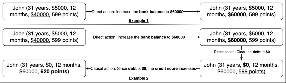
Figure 1: Example 1: John increases his bank balance to $\$60000$. Example 2: While the bank balance is directly altered by John, altering the credit score requires John to directly alter his debt obligations first. After clearing his debt, the causal effect of having $\$0$ debt increases John’s credit score to $620\ point$.

Example 2- Utility of Causal Actions: The extracted underlying logic of the classifier for loan rejection produces two rejection rules: 1) individuals with a bank balance of less than $\$60000$, and 2) individuals with a credit score below $600$. John (31 years, $\$5000$, $\$40000$, $599\ points$) is denied a loan (negative outcome) but wants approval (positive outcome). Without causal knowledge, the solution would be: Interventions: 1) Change the bank balance to $\$60000$, and 2) the credit score to $620\ points$. However, credit score cannot be changed directly. To realistically increase the credit score, the bank’s guidelines suggest having no debt, indicating a causal dependency between debt and credit score. CoGS provides: Initial state: John (31 years, $\$5000$, 12 months, $\$40000$, $599\ points$) is denied a loan. Goal state: John (31 years, $\$0$, 12 months, $\$60000$, $620\ points$) is approved for a loan. Interventions: 1) John changes his bank balance to $\$60000$, and 2) reduces his debt to $0 to increase his credit score. As shown in Figure 1, clearing the debt (direct action) leads to an increase in credit score, making John eligible for the loan. Intermediate states (e.g., ‘$\$5000$ in debt’ and ‘$\$0$ in debt’) represent the path to the goal state. Hence, we demonstrated how leveraging causal dependencies between features leads to realistic desired outcomes through appropriate interventions.

The challenge now is (i) identifying causal dependencies using rule-based machine learning algorithms (FOLD-SE), and (ii) computing the sequence of necessary interventions while avoiding repeating states— a known issue in the planning. CoGS addresses these by generating the path from the initial state i to the counterfactual goal state g using the find_path algorithm (Algorithm 2), explained in Section 4.2.1.

4 Methodology

We next outline the methodology used by CoGS to generate paths from the initial state (negative outcome) to the goal state (positive outcome). Unlike traditional planning problems where actions are typically independent, our approach involves interdependent actions governed by causal rules $C$. This ensures that the effect of one action can influence subsequent actions, making interventions realistic and causally consistent. Note that the CoGS framework uses the FOLD-SE RBML algorithm to automatically compute causal dependency rules. These rules have to be either verified by a human, or commonsense knowledge must be used to verify them automatically. This is important, as RBML algorithms can identify a correlation as a causal dependency. CoGS uses the former approach. We next define specific terms.

Definition 1 (State Space (S)).

$S$ represents all combinations of feature values. For domains $D_{1},...,D_{n}$ of the features $F_{1},...,F_{n}$, $S$ is a set of possible states $s$, where each state is defined as a tuple of feature values $V_{1},...,V_{n}$.

$$s\in S\ where\ S=\{(V_{1},V_{2},...,V_{n})\ |$$

$$V_{i}\in D_{i},\ for\ each\ i\ in\ 1,...,n\}$$

E.g., an individual John: s = $(31$ years, $\$5000$, $\$40000$, $599$ points$)$, where $s\in S$.

Definition 2 (Causally Consistent State Space ($S_{C}$)).

$S_{C}$ is a subset of $S$ where all causal rules are satisfied. $C$ represents a set of causal rules over the features within a state space $S$. Then, $\theta_{C}:P(S)\rightarrow P(S)$ (where $P(S)$ is the power set of S) is a function that defines the subset of a given state sub-space $S^{\prime}\subseteq S$ that satisfy all causal rules in C.

$$\theta_{C}(S^{\prime})=\{s\in S^{\prime}\mid s\ satisfies\ all\ causal\ rules\ in\ C\}$$

$$S_{C}=\theta_{C}(S)$$

E.g., causal rules state that if $debt$ is $0$, the credit score should be above 599, then instance $s_{1}$ = (31 years, $0, $40000, 620 points) is causally consistent, and instance $s_{2}$ = (31 years, $0, $40000, 400 points) is causally inconsistent.

In a traditional planning problem, allowed actions in a given state are independent, i.e., the result of one action does not influence another. In CoGS, causal actions are interdependent, governed by $C$.

Definition 3 (Decision Consistent State Space ($S_{Q}$)).

$S_{Q}$ is a subset of $S_{C}$ where all decision rules are satisfied. $Q$ represents a set of rules that compute some external decision for a given state. $\theta_{Q}:P(S)\rightarrow P(S)$ is a function that defines the subset of the causally consistent state space $S^{\prime}\subseteq S_{C}$ that is also consistent with decision rules in $Q$:

$$\theta_{Q}(S^{\prime})=\{s\in S^{\prime}\mid s\ satisfies\ any\ decision\ rule\ in\ Q\}$$

Given $S_{C}$ and $\theta_{Q}$, we define the decision consistent state space $S_{Q}$ as

$$S_{Q}=\theta_{Q}(S_{C})=\theta_{Q}(\theta_{C}(S))$$

E.g., an individual John whose loan has been rejected: s = ($31$ years, $\$0$, $\$40000$, $620$ points), where $s\in S_{Q}$.

Definition 4 (Initial State ($i$)).

$i$ is the starting point with an undesired outcome. Initial state $i$ is an element of the causally consistent state space $S_{C}$

$$i\in S_{C}$$

For example, $i=(31\ years,\ \$0,\ \$40000,\ 620\ points)$

Definition 5 (Actions).

The set of actions $A$ includes all possible interventions (actions) that can transition a state from one to another within the state space. Each action $a\in A$ is defined as a function that maps $s$ to a new state $s^{\prime}$.

$$a:S\rightarrow S\ \mid where\ a\in A$$

Actions are divided into: 1) Direct Actions: Directly change the value of a single feature of a state $s$, e.g., Increase bank balance from $\$40000$ to $\$60000$. 2) Causal Actions: Change the value of a target feature by altering related features, based on causal dependencies. It results in a causally consistent state with respect to C, e.g., reduce debt to increase the credit score.

Definition 6 (Transition Function).

A transition function $\delta:S_{C}\times A\rightarrow S_{C}$ maps a causally consistent state to the set of allowable causally consistent states that can be reached in a single step, and is defined as:

$$\delta(s,a)=\left\{\begin{array}[]{l}a(s)\textit{ if }a(s)\in S_{C}\\ \delta(a(s),a^{\prime})\textit{ with }a\in A,a^{\prime}\in A\textit{, otherwise}\end{array}\right.$$

$\delta$ models a function that repeatedly takes actions until a causally consistent state is reached. In example 1, $\delta$ suggests changing the bank balance from $\$40000$ to $\$60000$: $\delta(31\ years,\$5000,\$40000,599)=$ $(31\ years,\$5000,\$60000,599)$

Definition 7 (Counterfactual Generation (CFG) Problem).

A counterfactual generation (CFG) problem is a 4-tuple $(S_{C},S_{Q},I,\delta)$ where $S_{C}$ is causally consistent state space, $S_{Q}$ is the decision consistent state space, $I\in S_{C}$ is the initial state, and $\delta$ is a transition function.

Definition 8 (Goal Set).

The goal set $G$ is the set of desired outcomes that do not satisfy the decision rules $Q$. For the Counterfactual Generation (CFG) problem $(S_{C},S_{Q},I,\delta)$, $G\subseteq S_{C}$:

$$G=\{s\in S_{C}|s\not\in S_{Q}\}$$

$G$ includes all states in $S_{C}$ that do not satisfy $S_{Q}$. For example 1, an example goal state $g\in G$ is $g=(31\ years,\ \$5000,\ \$60000,\ 599\ points).$

Definition 9 (Solution Path).

A solution to the problem $(S_{C},S_{Q},I,\delta)$ with Goal set $G$ is a path:

$$s_{0},s_{1},\dots,s_{m}\ \text{where}\ s_{j}\in S_{C}\ \text{for all}\ j\in\{0,\dots,m\},$$

$$such\ that\ s_{0}=I;s_{m}=G;s_{0},...,s_{m-1}\not\in G;$$

$$s_{i+1}\in\delta(s_{i})\ \text{for}\ i\in\{0,\dots,m-1\}$$

For example 1, individuals with less than $\$60000$ in their account are ineligible for a loan, thus the state of an ineligible individual $s\in S_{Q}$ might be $s=(31\ years,\$5000,\$40000,599\ points)$. The goal set has only one goal state $g\in G$ given by $s=(31\ years,\$5000,\$60000,599\ points)$. The path from $s$ to $g$ is {(31 years,$5000,$40000,599 points)$\rightarrow Direct\rightarrow$(31 years,$5000,$60000,599 points)$\}$. Here, the path has only 2 states as only changing the bank balance to be $\$60000$ is needed to reach the goal state.

Algorithm 1 extract_logic: Extract the underlying logic of the classification model

0:  Original Classification model $M$, Data $H$, RBML Algorithm R:

1:  if  $M$ is rule-based then

2:     // Decision Rules are the rules of M

3:     Set Q = M

4:  else

5:     if  $M$ is statistical then

6:        // For input data H, predict the labels as V

7:        Set V = predict(M(H))

8:        // Use the H and V to train R

9:        Set R = train(R(H,V))

10:        // Decision Rules are the rules of R

11:        Set Q = R

12:     end if

13:  end if

14:  Return Q

4.1 Algorithm to Extract Decision Rules

We first describe the algorithm for extracting the underlying logic in the form of rules for the classification model that provides the undesired outcome. By using this extracted logic or rules, we can generate a path to the counterfactual solution $g$.

The function ‘extract_logic’ extracts the underlying logic of the classification model used for decision-making. Our CoGS framework applies specifically to tabular data, so any classifier handling tabular data can be used. Algorithm 1 provides the pseudocode for ‘extract_logic’, which takes the original classification model $M$, input data $H$, and a RBML algorithm $R$ as inputs and returns $Q$, the underlying logic of the classification model.

$Q$ represents the decision rules responsible for generating the undesired outcome. The algorithm first checks if the classification model $M$ is rule-based. If yes, we set $Q=M$ and return Q. Otherwise, the corresponding labels for the input data are predicted using $M$. These predicted labels, along with the input data $H$, are then used to train the RBML algorithm $R$. The trained RBML algorithm represents the underlying logic of $M$, and we set $Q=R$, returning $Q$ as the extracted decision rules.

4.2 Algorithm to Obtain the Counterfactual

We next describe our algorithm to find the goal states and compute the solution paths. The algorithm makes use of the following functions: (i) not_member: checks if an element is: a) not a member of a list, and b) Given a list of tuples, not a member of any tuple in the list. (ii) drop_inconsistent: given a list of states [$s_{0},...,s_{k}$] and a set of Causal rules $C$, it drops all the inconsistent states resulting in a list of consistent states with respect to $C$. (iii) get_last: returns the last member of a list. (iv) pop: returns the last member of a list. (v) is_counterfactual: returns True if the input state is a causally consistent counterfactual solution. (vi) intervene: performs interventions/ makes changes to the current state through a series of actions and returns a list of visited states. The interventions are causally compliant. Further details are available in the supplement.

Algorithm 2 find_path: Obtain a path to the counterfactual state

0:  Initial State $(I)$, States $S$, Causal Rules $C$, Decision Rules $Q$, is_counterfactual, intervene, Actions $a\in A$:

1:   Create an empty list visited_states that tracks the list of states traversed (so that we avoid revisiting them).

2:  Append ($i$, [ ]) to visited_states

3:  while is_counterfactual(get_last(visited_states),C,Q) is $FALSE$  do

4:     Set visited_states=intervene(visited_states,C,A)

5:  end while

6:  candidate_path = drop_inconsistent(visited_states)

7:  Return candidate_path

4.2.1 Find Path:

Function ‘find_path’ implements the Solution Path $P$ of Definition 9. Its purpose is to find a path to the counterfactual state. Algorithm 2 provides the pseudo-code for ‘find_path’, which takes as input an Initial State $i$, a set of Causal Rules $C$, decision rules $Q$, and actions $A$. It returns a path to the counterfactual state/goal state $g\in G$ for the given $i$ as a list ‘visited_states’. Unrealistic states are removed from ‘visited_states’ to obtain a ‘candidate_path’.

Initially, $s=i$. The function checks if the current state $s$ is a counterfactual. If $s$ is already a counterfactual, ‘find_path’ returns a list containing $s$. If not, the algorithm moves from $s=i$ to a new causally consistent state $s^{\prime}$ using the ‘intervene’ function, updating ‘visited_states’ with $s^{\prime}$. It then checks if $s^{\prime}$ is a counterfactual using ‘is_counterfactual’. If True, the algorithm drops all inconsistent states from ‘visited_states’ and returns the ‘candidate_path’ as the path from $i$ to $s^{\prime}$. If not, it updates ‘$current\_state$’ to $s^{\prime}$ and repeats until reaching a counterfactual/goal state $g$. The algorithm ends when ‘is_counterfactual’ is satisfied, i.e., $s^{\prime}=g\mid\ where\ g\in G$.

$$\begin{split}s^{\prime}\in G\mid\ by\ definition\\ s_{0},...,s_{k},s^{\prime}\mid s_{0},...,s_{k}:\not\in G\end{split}$$ (1)

4.2.2 Discussion:

A few points should be highlighted: (i) Certain feature values may be immutable or restricted, such as age cannot decrease or credit score cannot be directly altered. To respect these restrictions, we introduce plausibility constraints. These constraints apply to the actions in our algorithms, ensuring realistic changes to the features. Since they do not add new states but restrict reachable states, they are represented through the set of available actions in Algorithms 2, (ii) Similarly, CoGS has the ability to specify the path length for candidate solutions. Starting with a minimal path length of 1, CoGS can identify solutions requiring only a single change. If no solution exists, CoGS can incrementally increase the path length until a solution is found. This ensures that the generated counterfactuals are both minimal and causally consistent, enhancing their practicality and interpretability. This is achieved via constraints on path length.

4.3 Soundness

Definition 10 (CFG Implementation).

When Algorithm 2 is executed with the inputs: Initial State $i$ (Definition 4), States Space $S$ (Definition 1), Set of Causal Rules $C$ (Definition 2), Set of Decision Rules $Q$ (Definition 3), and Set of Actions $A$ (Definition 5), a CFG problem $(S_{C},S_{Q},I,\delta)$ (Definition 7) with causally consistent state space $S_{C}$ (Definition 2), Decision consistent state space $S_{Q}$ (Definition 3), Initial State $i$ (Definition 4), the transition function $\delta$ (Definition 6) is constructed.

Definition 11 (Candidate path).

Given the counterfactual $(S_{C},S_{Q},I,\delta)$ constructed from a run of algorithm 2, the return value (candidate path) is the resultant list obtained from removing all elements containing states $s^{\prime}\not\in S_{C}$.

Definition 10 maps the input of Algorithm 2 to a CFG problem (Definition 7). Candidate path maps the result of Algorithm 2 to a possible solution (Definition 9) of the corresponding CGF problem. From Theorem 1 (proof in supplement), the candidate path (Definition 11) is a solution to the corresponding CFG problem implementation (Definition 10).

Theorem 1 Soundness: Given a CFG $\mathbb{X}$=$(S_{C},S_{Q},I,\delta)$, constructed from a run of Algorithm 2 & a corresponding candidate path $P$, $P$ is a solution path for $\mathbb{X}$. Proof is provided in the supplement.

Dataset	Model	Fid. (%)	Acc. (%)	Prec. (%)	Rec. (%)	F1. (%)
Adult	DNN	N/A	85.57 $\pm$0.38	85.0 $\pm$0.63	85.8 $\pm$0.40	85.0 $\pm$0.63
	FOLD-SE[DNN]	93.16 $\pm$0.6	84.2 $\pm$0.28	83.4 $\pm$0.49	84.2 $\pm$0.4	83.4 $\pm$0.49
	GBC	N/A	86.45 $\pm$0.33	85.8 $\pm$0.4	86.6 $\pm$0.49	85.8 $\pm$0.4
	FOLD-SE[GBC]	95.94 $\pm$0.67	85.24 $\pm$0.23	84.6 $\pm$0.49	85.2 $\pm$0.4	84.2 $\pm$0.4
	RF	N/A	85.60 $\pm$0.27	85.0 $\pm$0.0	85.6 $\pm$0.49	85.2 $\pm$0.4
	FOLD-SE[RF]	90.27 $\pm$0.3	84.37 $\pm$0.23	83.4 $\pm$0.49	84.4 $\pm$0.49	83.2 $\pm$0.4
	LR	N/A	84.78 $\pm$0.28	84.2 $\pm$0.4	84.8 $\pm$0.4	84.2 $\pm$0.4
	FOLD-SE[LR]	94.03 $\pm$0.36	83.92 $\pm$0.32	83.0 $\pm$0.0	83.8 $\pm$0.40	83.4 $\pm$0.49
German	DNN	N/A	74.5 $\pm$1.67	73.0 $\pm$2.19	74.4 $\pm$1.74	73.0 $\pm$2.19
	FOLD-SE[DNN]	81.5 $\pm$2.32	71.6 $\pm$1.5	71.0 $\pm$2.37	71.6 $\pm$1.5	70.8 $\pm$1.72
	GBC	N/A	75.8 $\pm$1.63	74.6 $\pm$1.62	76.0 $\pm$1.67	74.6 $\pm$1.62
	FOLD-SE[GBC]	81.60 $\pm$5.42	72.6 $\pm$3.64	72.0 $\pm$2.9	72.6 $\pm$3.61	71.0 $\pm$3.03
	RF	N/A	75.7 $\pm$1.21	74.6 $\pm$2.15	76.0 $\pm$1.41	72.8 $\pm$1.17
	FOLD-SE[RF]	85.1 $\pm$2.37	71.6 $\pm$0.20	70.2 $\pm$1.94	71.2 $\pm$0.40	66.2 $\pm$2.86
	LR	N/A	74.5 $\pm$1.18	73.0 $\pm$1.26	74.6 $\pm$1.36	73.4 $\pm$1.02
	FOLD-SE[LR]	82.5 $\pm$2.41	72.2 $\pm$2.01	71.4 $\pm$2.87	72.0 $\pm$2.19	71.8 $\pm$2.48
Car	DNN	N/A	94.4 $\pm$0.31	97.6 $\pm$0.49	97.2 $\pm$0.40	97.2 $\pm$0.4
	FOLD-SE[DNN]	91.55 $\pm$3.95	91.6 $\pm$4.00	93.6 $\pm$2.5	91.6 $\pm$3.88	91.8 $\pm$3.87
	GBC	N/A	97.5 $\pm$1.12	97.4 $\pm$1.02	97.4 $\pm$1.02	97.4 $\pm$1.02
	FOLD-SE[GBC]	97.16 $\pm$3.8	95.24 $\pm$4.3	96.4 $\pm$2.8	95.4 $\pm$4.27	95.4 $\pm$4.27
	RF	N/A	95.71 $\pm$0.56	95.6 $\pm$0.8	95.6 $\pm$0.8	95.6 $\pm$0.8
	FOLD-SE[RF]	94.27 $\pm$3.27	95.08 $\pm$2.92	96.0 $\pm$2.19	95.2 $\pm$3.12	95.4 $\pm$2.87
	LR	N/A	94.79 $\pm$1.43	95.0 $\pm$1.79	94.8 $\pm$1.72	94.8 $\pm$1.72
	FOLD-SE[LR]	95.37 $\pm$1.21	94.32 $\pm$1.54	94.8 $\pm$1.17	94.4 $\pm$1.5	94.4 $\pm$1.5
Mushroom	DNN	N/A	100.0 $\pm$0.0	100.0 $\pm$0.0	100.0 $\pm$0.0	100.0 $\pm$0.0
	FOLD-SE[DNN]	99.57 $\pm$0.26	99.56 $\pm$0.25	99.4 $\pm$0.49	99.4 $\pm$0.49	99.4 $\pm$0.49
	GBC	N/A	99.95 $\pm$0.05	100.0 $\pm$0.0	100.0 $\pm$0.0	100.0 $\pm$0.0
	FOLD-SE[GBC]	99.57 $\pm$0.3	99.56 $\pm$0.25	99.4 $\pm$0.49	99.4 $\pm$0.49	99.4 $\pm$0.49
	RF	N/A	100.0 $\pm$0.0	100.0 $\pm$0.0	100.0 $\pm$0.0	100.0 $\pm$0.0
	FOLD-SE[RF]	99.57 $\pm$0.26	99.56 $\pm$0.25	99.4 $\pm$0.49	99.4 $\pm$0.49	99.4 $\pm$0.49
	LR	N/A	99.96 $\pm$0.05	100.0 $\pm$0.0	100.0 $\pm$0.0	100.0 $\pm$0.0
	FOLD-SE[LR]	99.6 $\pm$0.27	99.56 $\pm$0.25	99.4 $\pm$0.49	99.4 $\pm$0.49	99.4 $\pm$0.49

Table 1: Performance of FOLD-SE in learning the underlying logic of various models.

5 Experiments

We have split the tasks into two steps: 1) Find the rule based equivalent of the original model; and 2) Using the rules obtained, find the path to the counterfactual. Further details on the experiments as well as the implementation are provided in the supplement.

5.1 Approximation of Models

We demonstrate the utility of learning the underlying rules of any classifier using RBML algorithms. For our CoGS framework, we applied the FOLD-SE algorithm various classifiers, including Deep Neural Networks (DNN), Gradient Boosted Classifiers (GBC), Random Forest Classifiers (RF), and Logistic Regression Classifiers (LR). These classifiers are first trained on several datasets: the Adult dataset by Becker and Kohavi, (1996), the Statlog (German Credit) dataset by Hofmann, (1994), the Car evaluation dataset by Bohanec, (1997), and the Mushroom dataset by Schlimmer, (1981). The results of these classifiers and their corresponding FOLD-SE equivalent are shown in the Table 1. The Accuracy (Acc.), Precision (Prec.), Recall (Rec.) and F1 Score (F1.) performance on the test set are shown along with the Fidelity (Fid.) of the FOLD-SE approximation. Fidelity, as used by White and d’Avila Garcez, (2020), refers to the degree to which the RBML algorithm (FOLD-SE) approximates the behaviour of the underlying model. A higher fidelity score indicates that FOLD-SE closely matches the predictions of the underlying model.

FOLD-SE successfully learns the underlying logic of these models, and the decision rules it generates (denoted as $Q$ in Definition 3) are used to produce counterfactuals. While there is a penalty in performance compared to the original models, this is to be expected as FOLD-SE and other RBML algorithms have the added constraint of being explainable and interpretable in addition to learning the underlying logic when compared to the underlying models which may not have such constraints. For further details please see the supplement. Next we show how the decision rules learned by our RBML algorithm (FOLD-SE) are used to generate a path to the counterfactual.

5.2 Obtaining a Path to the Counterfactual

We applied the CoGS methodology to rules generated by FOLD-SE across the German, Adult, and Car Evaluation datasets. These datasets include demographic and decision labels such as credit risk (‘good’ or ‘bad’), income (‘$=<\$50k/year$’ or ‘$>\$50k/year$’), and used car acceptability. We relabeled the car evaluation dataset -‘acceptable’ or ‘unacceptable’- to generate the counterfactuals. For the German dataset, CoGS identifies paths that convert a ‘bad’ credit rating to ‘good’ to determine the criteria for a favourable credit risk, i.e., likely to be approved for a loan. Similarly, CoGS identifies paths for converting the undesired outcomes in the Adult and Car Evaluation datasets-‘$=<\$50k/year$’ and ‘unacceptable’-to their counterfactuals: ‘$>\$50k/year$’ and ‘acceptable’. We use CoGS to obtain counterfactual paths. Details are provided in the supplement.

Dataset	Avg. # Feature Values	Time (s)
Adult	2	$1.29\pm 0.43$
	2.667	$4.34\pm 3.60$
German	2.2	$8.98\pm 6.257$
	2.6	$27.82\pm 21.72$
Car	2	$1.29\pm 0.43$
	3	$15.49\pm 7.72$

Table 2: Scalability of CoGS: Time taken to generate a counterfactual path increases as Average Feature Values increases.

CoGS can be computationally heavy as it searches through an ever-increasing solution space to find a path to a counterfactual. We run an experiment to check the effect of increasing the search space of feature values on the time taken to obtain a counterfactual solution path. There are two ways to increase the search space: increase the number of features or, for a fixed set of features, increase the available values that can be assigned to them. Since our decision rules are static, so are our features. Hence, we increase the number of values available to the features and test its effect on the time taken. We only consider categorical features. This is because numeric features are handled as a range and are computationally treated as holding only one value —the range—hence, they have a limited effect on the feature space. We use a metric Average # Feature Values = (Total Count of Categorical Feature Values) $\div$ (Total Count of Categorical Features). Table 2 shows how increasing the Average Feature Values increases the time to find a solution. Further details of the experiment and counterfactual paths generated are available in the supplement.

6 Conclusion and Future Work

The main contribution of this paper is the CoGS framework, which automatically generates paths to causally consistent counterfactuals for any machine learning model—statistical or rule-based. CoGS efficiently computes counterfactuals, even for complex models, and the paths can be minimal if desired. By incorporating Answer Set Programming (ASP), CoGS ensures each counterfactual is causally compliant and delivered through a sequence of actionable interventions, making it more practical for real-world applications compared to methods by Bertossi and Reyes, (2021) and Karimi et al., (2021). Inspired by Padalkar et al., (2024), future work will explore improving scalability and extending CoGS to non-tabular data, such as image classification tasks.

References

- Arias et al., (2018) Arias, J., Carro, M., Salazar, E., Marple, K., and Gupta, G. (2018). Constraint Answer Set Programming without Grounding. TPLP, 18(3-4):337–354.
- Baral, (2003) Baral, C. (2003). Knowledge representation, reasoning and declarative problem solving. Cambridge University Press.
- Becker and Kohavi, (1996) Becker, B. and Kohavi, R. (1996). Adult. UCI Machine Learning Repository. DOI: https://doi.org/10.24432/C5XW20.
- Bertossi and Reyes, (2021) Bertossi, L. E. and Reyes, G. (2021). Answer-set programs for reasoning about counterfactual interventions and responsibility scores for classification. In Proc. ILP, LNCS.
- Bohanec, (1997) Bohanec, M. (1997). Car Evaluation. UCI Machine Learning Repository. DOI: https://doi.org/10.24432/C5JP48.
- Brewka et al., (2011) Brewka, G., Eiter, T., and Truszczynski, M. (2011). Answer set programming at a glance. Commun. ACM, 54(12):92–103.
- Byrne, (2019) Byrne, R. M. J. (2019). Counterfactuals in explainable artificial intelligence (XAI): evidence from human reasoning. In Proc. IJCAI, pages 6276–6282.
- Gelfond and Kahl, (2014) Gelfond, M. and Kahl, Y. (2014). Knowledge Representation, Reasoning, and the Design of Intelligent Agents: The Answer-Set Programming Approach. Cambridge University Press, USA.
- Hofmann, (1994) Hofmann, H. (1994). Statlog (German Credit Data). UCI Machine Learning Repository. DOI: https://doi.org/10.24432/C5NC77.
- Karimi et al., (2020) Karimi, A., Barthe, G., Balle, B., and Valera, I. (2020). Model-agnostic counterfactual explanations for consequential decisions. In AISTATS. PMLR.
- Karimi et al., (2021) Karimi, A., Schölkopf, B., and Valera, I. (2021). Algorithmic recourse: from counterfactual explanations to interventions. In Proc. ACM FAccT, pages 353–362.
- Padalkar et al., (2024) Padalkar, P., Wang, H., and Gupta, G. (2024). NeSyFOLD: A framework for interpretable image classification. In Proc. AAAI.
- Pearl, (2009) Pearl, J. (2009). Causal inference in statistics: An overview. Statistics Surveys, 3(none):96 – 146.
- Russell, (2019) Russell, C. (2019). Efficient search for diverse coherent explanations. In Proc. ACM FAT, page 20–28.
- Schlimmer, (1981) Schlimmer, J. (1981). Mushroom. UCI Machine Learning Repository. DOI: https://doi.org/10.24432/C5959T.
- Tolomei et al., (2017) Tolomei, G., Silvestri, F., Haines, A., and Lalmas, M. (2017). Interpretable predictions of tree-based ensembles via actionable feature tweaking. In Proc. ACM SIGKDD.
- Ustun et al., (2019) Ustun, B., Spangher, A., and Liu, Y. (2019). Actionable recourse in linear classification. In FAT. ACM.
- Wachter et al., (2018) Wachter, S., Mittelstadt, B., and Russell, C. (2018). Counterfactual explanations without opening the black box: Automated decisions and the gdpr.
- Wang and Gupta, (2024) Wang, H. and Gupta, G. (2024). FOLD-SE: an efficient rule-based machine learning algorithm with scalable explainability. In Proc. PADL 2024, pages 37–53. Springer LNCS 14512.
- White and d’Avila Garcez, (2020) White, A. and d’Avila Garcez, A. S. (2020). Measurable counterfactual local explanations for any classifier. In Proc. ECAI, volume 325, pages 2529–2535.