Ising Disks

Abstract.

We introduce a dynamic model where the state space is the set of contractible cubical sets in the Euclidian space. The permissible state transitions, that is addition and removal of a cube to/from the set, is locally decidable. We prove that in the planar special case the state space is connected. We then define a continuous time Markov chain with a fugacity (tendency to grow) parameter. We prove that, on the plane, the Markov chain is irreducible (due to state connectivity), and is also ergodic if the fugacity is smaller than a threshold.

1. Introduction

A cubical set (complex) is a collection of cubes (i.e., products of unit intervals, of various dimensions) such that the intersection of any two cubes is again within the collection. In this paper, we will be dealing with complexes formed by the $d$-dimensional cubes of the integer partition of $\mathbb{R}^{d}$, cubes that are products of intervals that start and end at integers in $d$ copies of the real line. Equivalently, we will be dealing with the subsets of the cube-centered lattice.

We will be looking at the Markov chains valued in such cubical sets, defined by a Glauber-like local dynamics, generating, in essence, a topologically constrained Ising model.

An important constraint on the cubical set of our model is that their topology will be fixed: the homotopy type of the union of (closed) cubes of the complex will remain constant. In the following we will be initiating the process with a single cube, so that throughout the evolution, the cubical set will remain contractible. Of course, one can start with arbitrary topological homotopy type realizable by a cubical set in $\mathbb{R}^{d}$.

It might be surprising that this constraint can be realized using local updates: for example, that would be impossible if one attempted to keep the configuration merely connected. However, as we show, the homotopy type can be preserved under the local moves, resulting in an ensemble of contractible cubical complexes. In fact, we will be working with a version where even the local relative homology of any boundary point of the cubical complex $\mathbf{X}$ modulo its small vicinity (in $\mathbf{X}$) is contractible, thus making the union of the cubes homeomorphic to the $d$-disk. We call such cubical sets clumps.

In the case of planar clumps, their boundary forms a self-avoiding planar polygon, a close relative of the self-avoiding polygons, a highly studied object in statistical physics. Our construction allows one to generate higher-dimensional analogues to self-avoiding walks, - self avoiding codimension $1$ cellular structures, something that has not been explored thus far.

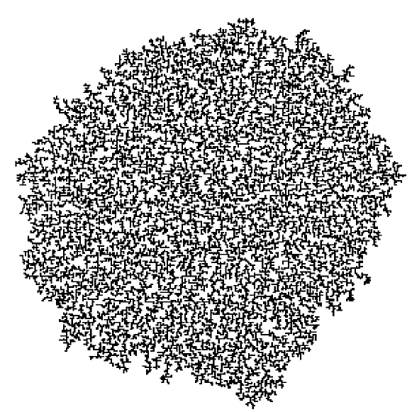
Figure 1.1. A planar clump, generated by the Markov process defined in Section 6 in the over-critical regime.

While our model is, we believe, new, there are several adjacent lines of research. One of them addresses the self-avoiding paths and polygons [guttbook, guttmann_self-avoiding_2012]. The other deals with the general growth models, and their topology. In a recent paper [damron_number_2023], the authors consider the shape emerging by time $t$ in the last passage percolation model, and ask what is the number of holes in (equivalently, what is the $(d-1)$-th Betti number of) the resulting shape. More detailed results about the topology of that shape are obtained in [manin_topology_2023, hua_local_2024]. Again, the emphasis in this line of research is to describe the local topology in the growth models, rather than to generate a topology-constrained one.

In this paper, we are focusing on the few basic patterns of the clumps: construction, phase transition in $d=2$, and some large deviation estimates. The model, however, is rich, and invites a number of different questions.

One of them is the question of the shapes of the clumps. One way to think about them is to view them as two counteracting drifts: to grow, driven by the entropic factor, i.e., the number of clump configurations growing exponentially, as $\mu^{A},\mu>1$, in the surface area $A$, and the fugacity, which controls the growth exponentially in the volume. As the volume cannot grow more slowly than the surface area of the clump, there is a phase transition: when the fugacity is below a threshold, $\kappa_{*}$, the clump remains bounded. Furthermore, in the over-critical regime, when the fugacity is not too high, the clumps grow in a porous fashion, looking like a coral (or vesicle [guttmann_self-avoiding_2012]), see Fig. 1.1. It would be instructive to quantify this behavior.

While we focus here on the clumps evolving from a single cube, other starting configurations are possible. One version of interest is to start with a half space occupied, half vacant. A coral-like interface develops: what is its typical width? speed? These and many other questions will be addressed elsewhere.

2. Cubical Set Definitions and Notation

Some of the standard definitions we include in the coming paragraphs, and will use throughout the paper, are from [mischai], although there are some important differences.

An elementary interval is a set in the form of either $[l-\frac{1}{2},l+\frac{1}{2}]$ or $\{l+\frac{1}{2}\}$ for $l\in\mathbb{Z}$. It is called non-degenerate if it is in the $[l-\frac{1}{2},l+\frac{1}{2}]$ form, and degenerate otherwise. For some fixed $d\geq 2$, an (elementary) cube, $X$, is defined as a product of $d$ elementary intervals. We refer to the geometric realization of a given cube $X$ in the Euclidian space as $|X|\subset\mathbb{R}^{d}$. All cube realizations we consider will be in $\mathbb{R}^{d}$.

We call an elementary cube $k$-dimensional if exactly $k$ of the elementary intervals that compose it are non-degenerate. The set of all elementary cubes of dimension $j\geq 0$ is denoted by $\mathcal{K}^{j}$. With some abuse of notation, for $X,Y\in\mathcal{K}^{j}$, we mean by $X\cap Y\in\mathcal{K}^{i}$ that $|X|\cap|Y|$ is the geometric realization of an $i$-dimensional elementary cube in $\mathbb{R}^{d}$. We will also say that $X$ and $Y$ share an $i$-dimensional face in this case.

We call the point in $\mathbb{R}^{d}$ obtained through taking the middle point of each elementary interval that composes a cube $X$, the center of $X$, and denote it by $\operatorname{\mathtt{c}}(X)$. For instance, the center of the cube $[-\frac{1}{2},\frac{1}{2}]\times\{\frac{3}{2}\}$ is the point $(0\;\;\frac{3}{2})\in\mathbb{R}^{2}$.

A cubical set, $\mathbf{X}=\{X_{1},\ldots,X_{m}\}$ for $m\geq 2$, is any finite subset of $\mathcal{K}^{d}$. The cardinality of a cubical set will be denoted by $\operatorname{\mathtt{card}}(\mathbf{X})$, whereas $|\mathbf{X}|$ will denote its geometric realization, i.e.,

$$|\mathbf{X}|\coloneqq\bigcup_{i=1}^{m}|X_{i}|.$$

For an $x\in\mathbb{R}^{d}$, $\|x\|_{2}$ and $\|x\|_{\infty}$ denote the $\ell_{2}$ and $\ell_{\infty}$ norms respectively. We denote the ball in terms of the $\ell_{2}$ norm centered at $x\in\mathbb{R}^{d}$ of radius $\varepsilon$ by $B_{\varepsilon}(x)$. We denote the set of nonnegative reals by $\mathbb{R}^{+}$ and the set of nonnegative integers by $\mathbb{N}$.

3. More Definitions and Fundamentals

In addition to the standard definitions given in the previous section, here, we introduce some new concepts that we will use to study contractible cubical sets.

Definition 3.1 (Regularity).

Given a subset $\mathscr{A}$ of $\mathbb{R}^{d}$, a point $x\in\mathscr{A}$ is called a regular point of $\mathscr{A}$, if and only if it satisfies at least one of the following conditions.

1. It is an interior point of $\mathscr{A}$, i.e., $\exists\varepsilon>0$ such that

   $$B_{\varepsilon}(x)\subset\mathscr{A}.$$

2. The set

   $$B_{\varepsilon}(x)\cap\mathscr{A}\setminus\{x\}$$

   is contractible (homotopy equivalent to a single point) for all $\varepsilon>0$ small enough.

Definition 3.2.

A cubical set $\mathbf{X}$ is called a regular cubical set if all $x\in|\mathbf{X}|$ is a regular point of $|\mathbf{X}|$.

Example 3.3.

For $d=2$ and $d=3$, some examples of irregular points are illustrated in Figure 3.2.

Figure 3.2. Illustration of irregular points for $d=2$ and $d=3$

Remark 3.4.

Note that regularity is a local property. That is, for an $x\in\mathscr{A}\cup\mathscr{B}$ with $\mathscr{A},\mathscr{B}\subset\mathbb{R}^{d}$, if

$$B_{\varepsilon}(x)\cap\mathscr{A}=B_{\varepsilon}(x)\cap\mathscr{B}$$ (3.1)

for all $\varepsilon>0$ small enough, then $x$ is a regular point of $\mathscr{A}$ if and only if it is a regular point of $\mathscr{B}$.

Definition 3.5 (Neighborhood and Perimeter).

Given a cubical set $\mathbf{X}$ and $X\in\mathcal{K}^{d}$, we call the cubical set

$$\mathcal{N}_{\mathbf{X}}(X)\coloneqq X\cup\left\{\bigcup_{\stackrel{{\scriptstyle Y\in\mathbf{X}}}{{|Y|\cap|X|\neq\varnothing}}}Y\right\}$$

the neighborhood of $X$ in $\mathbf{X}$. We will also sometimes refer to the geometric realization $|\mathcal{N}_{\mathbf{X}}(X)|$ as the neighborhood when the context is clear.

Remark 3.6.

Note that

$$|\mathcal{N}_{\mathbf{X}}(X)|=|X|\cup\left\{y\in|\mathbf{X}|:\|y-\operatorname{\mathtt{c}}(X)\|_{\infty}\leq\frac{3}{2}\right\}.$$

Definition 3.7.

The perimeter of the neighborhood $|\mathcal{N}_{\mathbf{X}}(X)|$ is defined as the set

$$\left\{y\in|\mathcal{N}_{\mathbf{X}}(X)|:\|y-\operatorname{\mathtt{c}}(X)\|_{\infty}=\frac{3}{2}\right\}.$$

Next, we give our first observation regarding irregularity, which shows that irregular points of a neighborhood should be “inside” of it.

Lemma 3.8.

For any cubical set $\mathbf{X}$ and $X\in\mathcal{K}^{d}$, the neighborhood $|\mathcal{N}_{\mathbf{X}}(X)|$ cannot have an irregular point on its perimeter.

Proof.

Assume $x=(x_{1},\ldots,x_{d})$ is an irregular point of $|\mathcal{N}_{\mathbf{X}}(X)|$ on its perimeter. Also assume, without loss of generality, that $x$ is on the hyperplane $\left\{z+\frac{1}{2}\right\}\times\mathbb{R}^{d-1}$ for some $z\in\mathbb{Z}$, and that for all $\varepsilon$ small enough,

$$(x_{1},x_{1}+\varepsilon]\times\{x_{2}\}\times\ldots\times\{x_{d}\}\subset|\mathcal{N}_{\mathbf{X}}(X)|,$$

while

$$[x_{1}-\varepsilon,x_{1})\times\{x_{2}\}\times\ldots\times\{x_{d}\}$$

does not intersect $|\mathcal{N}_{\mathbf{X}}(X)|$. We observe that for every $d$-dimensional cube $Y\in\mathcal{N}_{\mathbf{X}}(X)$ with $x\in|Y|$,

$$(x_{1},x_{1}+\varepsilon]\times\{x_{2}\}\times\ldots\times\{x_{d}\}\subset|Y|,$$

and therefore, $B_{\varepsilon}(x)\cap|Y|\setminus\{x\}$ has a deformation retraction to $(x_{1},x_{1}+\varepsilon]\times\{x_{2}\}\times\ldots\times\{x_{d}\}$. Since

$$B_{\varepsilon}(x)\cap|\mathcal{N}_{\mathbf{X}}(X)|\setminus\{x\}=\bigcup_{Y\in\mathcal{N}_{\mathbf{X}}(X)}B_{\varepsilon}(x)\cap|Y|\setminus\{x\},$$

and each set that composes the union on the right hand side has a deformation retraction to $(x_{1},x_{1}+\varepsilon]\times\{x_{2}\}\times\ldots\times\{x_{d}\}$, which is contractible, we conclude $B_{\varepsilon}(x)\cap|\mathcal{N}_{\mathbf{X}}(X)|\setminus\{x\}$ has to be contractible. This, however, is in contradiction with our initial assumption that $x$ was an irregular point of $|\mathcal{N}_{\mathbf{X}}(X)|$, concluding the proof. ∎

We establish in the lemma below that regularity of a cubical set is equivalent to the local regularity of the neighborhoods of its cubes.

Lemma 3.9.

The cubical set $\mathbf{X}$ is regular if and only if $\mathcal{N}_{\mathbf{X}}(X)$ is so for all $X\in\mathbf{X}$.

Proof.

Assume $x\in\mathbb{R}^{d}$ is an irregular point of $|\mathcal{N}_{\mathbf{X}}(X)|$. This requires $x$ be not in the perimeter of $|\mathcal{N}_{\mathbf{X}}(X)|$ due to Lemma 3.8. For all such $x$, though, (3.1) holds for $\mathscr{A}=|\mathcal{N}_{\mathbf{X}}(X)|$ and $\mathscr{B}=|\mathbf{X}|$, and therefore $x$ is an irregular point of $|\mathbf{X}|$ as well, which implies $\mathbf{X}$ is irregular.

Assume now that $x$ is an irregular point of $|\mathbf{X}|$. Choose an arbitrary $X\in\mathbf{X}$ such that $x\in|X|$. Using Remark 3.4 again for the same choice of $\mathscr{A}$ and $\mathscr{B}$ as above, we conclude $x$ is also an irregular point of $|\mathcal{N}_{\mathbf{X}}(X)|$. We proved if $x$ is an irregular point of $|\mathcal{N}_{\mathbf{X}}(X)|$ then it is also an irregular point of $|\mathbf{X}|$, and if $x$ is an irregular point of $\mathbf{X}$ then there exists $X\in\mathbf{X}$ such that it is irregular in $|\mathcal{N}_{\mathbf{X}}(X)|$. These two assertions prove the claim in the lemma. ∎

4. Clumps

We define below the main object of study in this paper, and the partial order on them underlying the Markov process we will define.

Definition 4.1 (Clump).

A cubical set $\mathbf{X}$ is called a clump if it is regular and its geometric realization $|\mathbf{X}|$ is contractible.

Definition 4.2 (Collapse).

Given a cubical set $\mathbf{X}$, $\operatorname{\mathtt{card}}(\mathbf{X})\geq 2$ and a cube $X\in\mathbf{X}$, we call the cubical set $\mathbf{X}\setminus X$ the collapse of $\mathbf{X}$ through $X$.

Definition 4.3 ($k$-Collapsibility).

A clump $\mathbf{X}$ is called $k$-collapsible if there exist distinct cubes $X_{1},\ldots,X_{k}\in\mathbf{X}$ such that $\mathbf{X}\setminus X_{i}$ is a clump for each $i\in\{1,\ldots,k\}$. We say that $\mathbf{X}$ is collapsible “to $\mathbf{X}\setminus X_{i}$” or “through $X_{i}$” for any $i\in\{1,\ldots,k\}$, and call the set $\{X_{1},\ldots,X_{k}\}$ its collapse set. We call 1-collapsible clumps, sometimes, briefly, collapsible. When we say that the neighborhood $\mathcal{N}_{\mathbf{X}}(X)$ is collapsible we mean it is a clump and it is collapsible through $X$.

Figure 4.3. Collapse action for a cubical set in $\mathbb{R}^{2}$

The following lemma establishes that collapsibility through a cube is a neighborhood property. This will make sure that the rules of actions of our dynamic model for cubical sets that we will define later on will be local.

Lemma 4.4.

The clump $\mathbf{X}$ is collapsible through some $X\in\mathbf{X}$ if and only if $\mathcal{N}_{\mathbf{X}}(X)$ is a collapsible clump.

Proof.

We first prove the “if” part. Assume for an $X\in\mathbf{X}$, $\mathcal{N}_{\mathbf{X}}(X)$ is a collapsible clump, which implies $\mathcal{N}_{\mathbf{X}}(X)\setminus X$ is regular. We will first show that $\mathbf{X}\setminus X$ is regular. For that, take a point $x\in|\mathbf{X}\setminus X|$. If $x\in|X|$, using Remark 3.4 with the choices of $\mathscr{A}=|\mathbf{X}\setminus X|$ and $\mathscr{B}=|\mathcal{N}_{\mathbf{X}}(X)\setminus X|$, and that $\mathcal{N}_{\mathbf{X}}(X)\setminus X$ is regular, $x$ has to be regular in $|\mathbf{X}\setminus X|$. Assume now that $x\notin|X|$. Now using Remark 3.4 for $\mathscr{A}=|\mathbf{X}\setminus X|$, $\mathscr{B}=|\mathbf{X}|$, and that $\mathbf{X}$ was regular, we obtain that $x$ is regular in $|\mathbf{X}\setminus X|$. This concludes the proof that $\mathbf{X}\setminus X$ is regular.

To prove that the collapse of $\mathbf{X}$ through $X$ is contractible, we take a deformation retraction $F(x,t):|\mathbf{X}|\times[0,1]\to|\mathbf{X}|$ from $|\mathbf{X}|$ to a point $y\in|\mathcal{N}_{\mathbf{X}}(X)\setminus X|$, existence of which is implied by the fact that $\mathbf{X}$ is a clump. Also take a deformation retraction from $|\mathcal{N}_{\mathbf{X}}(X)\setminus X|$ to the point $y$, $\tilde{F}(x,t):|\mathcal{N}_{\mathbf{X}}(X)\setminus X|\times[0,1]\to|\mathcal{N}_{\mathbf{X}}(X)\setminus X|$, where $\tilde{F}(x,1)=y$ for all $x\in|\mathcal{N}_{\mathbf{X}}(X)\setminus X|$. Note such $\tilde{F}$ exists since $\mathcal{N}_{\mathbf{X}}(X)$ is a collapsible clump (through $X$) and therefore $|\mathcal{N}_{\mathbf{X}}(X)\setminus X|$ is contractible. Furthermore, for each $x\in|\mathbf{X}\setminus X|$, define

$$T_{x}\coloneqq\inf\left\{t\in[0,1]\,\,|\,\,F(x,t)\in\mathcal{N}_{\mathbf{X}}(X)\right\}.$$

Trivially, $T_{x}=0$ for all $x\in|\mathcal{N}_{\mathbf{X}}(X)\setminus X|$. Now we define the mapping $G:|\mathbf{X}\setminus X|\times[0,1]\to|\mathbf{X}\setminus X|$

$$G(x,t)=\begin{cases}F(x,t)\quad&\text{if}\quad t<T_{x}\\ \tilde{F}\left(F(x,T_{x}),\frac{t-T_{x}}{1-T_{x}}\right)&\text{otherwise.}\end{cases}$$ (4.1)

Note that $G(x,t)$ is continuous since $F$ and $\tilde{F}$ are and $G(x,0)$ and $G(x,1)=y$ for all $x\in|\mathbf{X}\setminus X|$. Therefore $G$ defines a homotopy between the identity $\text{id}_{|\mathbf{X}\setminus X|}$ and the constant map $y$, establishing that $|\mathbf{X}\setminus X|$ is contractible. Together with the regularity, this establishes that $\mathbf{X}\setminus X$ is a clump, and therefore, $\mathbf{X}$ is collapsible through $X$.

To prove the reverse implication, assume $\mathbf{X}$ is a collapsible clump through some $X\in\mathbf{X}$. For the regularity of $\mathcal{N}_{\mathbf{X}}(X)\setminus X$, take an $x\in|\mathcal{N}_{\mathbf{X}}(X)\setminus X|$. If $x$ is on the perimeter of $|\mathcal{N}_{\mathbf{X}}(X)\setminus X|$, then $x$ is regular in $|\mathcal{N}_{\mathbf{X}}(X)\setminus X|$ due to Lemma 3.8. If otherwise $x$ is not on the perimeter of $|\mathcal{N}_{\mathbf{X}}(X)\setminus X|$, we invoke Remark 3.4 for $\mathscr{A}=|\mathbf{X}\setminus X|$ and $\mathscr{B}=|\mathcal{N}_{\mathbf{X}}(X)\setminus X|$ to conclude $x$ is regular in $|\mathcal{N}_{\mathbf{X}}(X)\setminus X|$. This concludes the proof that $\mathcal{N}_{\mathbf{X}}(X)\setminus X$ is regular. Repeating the argument with some $x\in|\mathcal{N}_{\mathbf{X}}(X)|$ with $\mathscr{A}=|\mathbf{X}|$ and $\mathscr{B}=|\mathcal{N}_{\mathbf{X}}(X)|$ proves that $\mathcal{N}_{\mathbf{X}}(X)$ is also regular.

For the contractibility, assume $|\mathcal{N}_{\mathbf{X}}(X)\setminus X|$ is not contractible. This means that $|\mathcal{N}_{\mathbf{X}}(X)\setminus X|$ bounds a non-contractible $d^{\prime}$-dimensional hole for some $d^{\prime}\leq d$. Note that, by definition, $|\mathbf{X}\setminus X|$ bounds the same hole and therefore it has to be uncontractible as well, contradicting the assumption that $\mathbf{X}$ was a collapsible clump through $X$. Repeating the arguments for $|\mathcal{N}_{\mathbf{X}}(X)|$ and $|\mathbf{X}|$ establishes that $|\mathcal{N}_{\mathbf{X}}(X)|$ also has to be contractible. Since both $\mathcal{N}_{\mathbf{X}}(X)$ and $\mathcal{N}_{\mathbf{X}}(X)\setminus X$ are regular and their geometric realizations are contractible, we conclude that $\mathcal{N}_{\mathbf{X}}(X)$ is a collapsible clump. ∎

Below, we define the inverse of the collapse action, expansion.

Definition 4.5 (Expand).

Given a cubical set $\mathbf{X}$, $\operatorname{\mathtt{card}}(\mathbf{X})\geq 1$ and a cube $Y\in\mathcal{K}^{d}\setminus\mathbf{X}$, we call the cubical set $\mathbf{X}\cup Y$ the expansion of $\mathbf{X}$ through $Y$. A clump $\mathbf{X}$ is called expandable through $Y\in\mathcal{K}^{d}\setminus\mathbf{X}$ if $\mathbf{X}\cup Y$ is a clump.

That a clump $\mathbf{X}$ is expandable or not is also a neighborhood property, as expected, which is shown in the next lemma.

Lemma 4.6.

The clump $\mathbf{X}$ is expandable through some $Y\in\mathcal{K}^{d}$ if and only if $\mathcal{N}_{\mathbf{X}}(Y)$ is a collapsible clump and $Y\notin\mathbf{X}$.

Proof.

Assume first that $\mathcal{N}_{\mathbf{X}}(Y)$ is a collapsible clump for some $Y\in\mathcal{K}^{d}\setminus\mathbf{X}$ and $\mathbf{X}$ is a clump. Proof of the regularity of $\mathbf{X}\cup Y$ follows the same arguments presented in the first paragraph of the proof of Lemma 4.4 with appropriate choices for the sets $\mathscr{A}$ and $\mathscr{B}$. Namely, we choose $\mathscr{A}=|\mathbf{X}\cup Y|$, $\mathscr{B}=|\mathcal{N}_{\mathbf{X}}(Y)|$ if $x\in|Y|$, and $\mathscr{A}=|\mathbf{X}\cup Y|$, $\mathscr{B}=|\mathbf{X}|$ otherwise. Proof that $|\mathbf{X}\cup Y|$ is contractible follows by the analogous arguments to the second paragraph of the proof of Lemma 4.4, choosing some $y\in|\mathcal{N}_{\mathbf{X}}(Y)\setminus Y|$ and a deformation retraction $\tilde{F}(x,t):|\mathcal{N}_{\mathbf{X}}(Y)|\times[0,1]\to|\mathcal{N}_{\mathbf{X}}(Y)|$ and using that $|\mathbf{X}|$ and $|\mathcal{N}_{\mathbf{X}}(Y)|$ are contractible. Defining the mapping $G:|\mathbf{X}\cup Y|\times[0,1]\to|\mathbf{X}\cup Y|$ as in (4.1), we see that $G$ is a homotopy between $\text{id}_{|\mathbf{X}\cup Y|}$ and the constant map $y$, establishing that $|\mathbf{X}\cup Y|$ is contractible and therefore a clump.

The reverse implication is similar to the argument in the last two paragraphs of the proof of Lemma 4.4. Namely, assume $\mathbf{X}$ is expandable through $Y\in\mathcal{K}^{d}\setminus\mathbf{X}$. Take an $x\in|\mathcal{N}_{\mathbf{X}}(Y)|$ but not on the perimeter. Using Remark 3.4 with $\mathscr{A}=|\mathbf{X}\cup Y|$, $\mathscr{B}=|\mathcal{N}_{\mathbf{X}}(Y)|$ reveals $x$, and therefore, $\mathcal{N}_{\mathbf{X}}(Y)$ is regular. Repeating this with $x\in|\mathcal{N}_{\mathbf{X}}(Y)\setminus Y|$, $\mathscr{A}=|\mathbf{X}|$, $\mathscr{B}=|\mathcal{N}_{\mathbf{X}}(Y)\setminus Y|$ lets us conclude $\mathcal{N}_{\mathbf{X}}(Y)\setminus Y$ is regular too. For conciseness, the proof that both $|\mathcal{N}_{\mathbf{X}}(Y)|$ and $|\mathcal{N}_{\mathbf{X}}(Y)\setminus Y|$ are contractible is omitted. ∎

Combining Lemma 4.4 and Lemma 4.6 we can state the following corollary.

Corollary 4.7.

The clump $\mathbf{X}$ is expandable through some $Y\in\mathcal{K}^{d}\setminus\mathbf{X}$ if and only if $\mathbf{X}\cup Y$ is a collapsible clump through $Y$.

Next, we give definitions that we will use in our study of cubical sets when $d=2$. We establish the definitions in any $d$, for the sake of generality, nevertheless.

Definition 4.8 (Paths and Loops).

A sequence of distinct $d$-dimensional elementary cubes $P_{1},\ldots,P_{n}$ is called a path (of length $n\geq 2$) if $P_{i}\cap P_{i+1}\in\mathcal{K}^{d-1}$ for all $1\leq i\leq n-1$. The path $P_{1},\ldots,P_{n}$ is a loop if $P_{1}\cap P_{n}\in\mathcal{K}^{d-1}$ and $n\geq 3$. The term “path” will sometimes refer to the cubical set $\mathbf{P}\coloneqq\{P_{1},\ldots,P_{n}\}$ when there is no room for confusion. We say a path $\mathbf{P}$ is in the cubical set $\mathbf{X}$ if $\mathbf{P}\subseteq\mathbf{X}$.

Definition 4.9 (Nerve).

Given a path $\mathbf{P}=\{P_{1},\ldots,P_{n}\}$, we call the set

$$\operatorname{\mathtt{nrv}}(\mathbf{P})\coloneqq\begin{cases}\left\{\bigcup_{i=1}^{n-1}\mkern 1.5mu\overline{\mkern-1.5mu\operatorname{\mathtt{c}}(P_{i})\operatorname{\mathtt{c}}(P_{i+1})\mkern-1.5mu}\mkern 1.5mu\right\}\cup\mkern 1.5mu\overline{\mkern-1.5mu\operatorname{\mathtt{c}}(P_{n})\operatorname{\mathtt{c}}(P_{1})\mkern-1.5mu}\mkern 1.5mu\quad&\text{if $\mathbf{P}$ is a loop},\\ \bigcup_{i=1}^{n-1}\mkern 1.5mu\overline{\mkern-1.5mu\operatorname{\mathtt{c}}(P_{i})\operatorname{\mathtt{c}}(P_{i+1})\mkern-1.5mu}\mkern 1.5mu&\text{otherwise.}\end{cases}$$

the nerve of $\mathbf{P}$, where $\mkern 1.5mu\overline{\mkern-1.5muab\mkern-1.5mu}\mkern 1.5mu\subset\mathbb{R}^{d}$ denotes the closed line segment connecting $a,b\in\mathbb{R}^{d}$.

We have a similar definition for general cubical sets as follows.

Definition 4.10 (Skeleton).

Given a cubical set $\mathbf{X}$ we call the set

$$\left\{\bigcup_{X\in\mathbf{X}}\operatorname{\mathtt{c}}(X)\right\}\cup\left\{\bigcup_{\stackrel{{\scriptstyle X,Y\in\mathbf{X}}}{{X\cap Y\in\mathcal{K}^{d-1}}}}\mkern 1.5mu\overline{\mkern-1.5mu\operatorname{\mathtt{c}}(X)\operatorname{\mathtt{c}}(Y)\mkern-1.5mu}\mkern 1.5mu\right\}$$

the skeleton of $\mathbf{X}$.

We next define a concept only for $d=2$ case, to be used in the next section.

Definition 4.11 (Interior, $d=2$).

Given a loop $\mathbf{L}$, composed of subsequent distinct cubes $L_{1},\ldots L_{n}$, we define its interior, $\operatorname{\mathtt{int}}(\mathbf{L})\subset\mathbb{R}^{2}$, as the union of $|\mathbf{L}|$ and the subset of $\mathbb{R}^{2}$ bounded by its nerve.

Now that we have established the fundamentals of clumps and actions defined on them, we are ready to focus on the planar special case $(d=2)$, where we can prove some stronger statements.

5. Planar Clumps

We state our first main theorem below.

Theorem 5.1.

For $d=2$, all clumps are 2-collapsible.

Remark 5.2.

Note that 2-collapsibility is the strongest notion of collapsibility that can be proven for all clumps of all sizes on the plane. The “straight line” clump shown in the Figure 5.4 below can be made arbitrarily large, but although it is 2-collapsible (through first and last cubes), it is never 3-collapsible.

Figure 5.4. Line clump.

Before giving the proof of the theorem, we will give some auxiliary lemmas. Unless otherwise noted, we assume $d=2$ for the rest of this section. We start with definitions of some specific cubical sets that will play an important role in our proof of Theorem 5.1. Note that for the rest of this section, we will continue calling our building blocks “cubes” in order to be consistent with the general notation, although one might argue calling them “squares” would have been more intuitive.

Definition 5.3 (Rectangle Configuration).

We define the 2-by-3 rectangle configuration as the cubical set $\mathbf{R}_{6}$ composed of 6 cubes (illustrated in Figure 5.5). More concretely,

$$\begin{split}\mathbf{R}_{6}\coloneqq&\bigg{\{}\left[-\frac{3}{2},-\frac{1}{2}\right]\times\left[\frac{1}{2},\frac{3}{2}\right],\left[-\frac{1}{2},\frac{1}{2}\right]\times\left[\frac{1}{2},\frac{3}{2}\right],\left[\frac{1}{2},\frac{3}{2}\right]\times\left[\frac{1}{2},\frac{3}{2}\right],\\ &\left[-\frac{3}{2},-\frac{1}{2}\right]\times\left[-\frac{1}{2},\frac{1}{2}\right],\left[-\frac{1}{2},\frac{1}{2}\right]\times\left[-\frac{1}{2},\frac{1}{2}\right],\left[\frac{1}{2},\frac{3}{2}\right]\times\left[-\frac{1}{2},\frac{1}{2}\right]\bigg{\}}.\end{split}$$

Figure 5.5. 2-by-3 rectangle configuration $\mathbf{R}_{6}$ with the origin of $\mathbb{R}^{2}$ for reference.

We call the 90-degree rotational symmetry of $\mathbf{R}_{6}$, defined in a straightforward way, $\mathbf{R}_{6}^{\top}$, which is illustrated in Figure 5.6.

Figure 5.6. Rotational symmetry of $\mathbf{R}_{6}$, i.e., $\mathbf{R}_{6}^{\top}$

We say that a cubical set $\mathbf{X}$ includes (or does have) a 2-by-3 rectangle (at $z$) if there exists $z\in\mathbb{Z}^{2}$ such that

$$\mathbf{X}\supseteq\mathbf{R}_{6}+z$$

or

$$\mathbf{X}\supseteq\mathbf{R}_{6}^{\top}+z,$$

where $\mathbf{X}+z$ is the translation of $\mathbf{X}$ defined in the natural way.

Definition 5.4 (Double-deck Configuration).

The cubical set double-deck configuration is shown in Figure 5.7. A formal definition is straightforward and omitted to save space.

Figure 5.7. Double-deck configuration at the origin (0,0).

We adopt the same terminology we introduced previously for the rectangular configuration. That is, we say a cubical set has a double-deck (configuration) if it includes a translation or rotation of a double deck at $(0,0)$.

Definition 5.5 (Human Configuration).

The cubical set Human configuration, named after its resemblance to the silhouette of the human body, is shown in Figure 5.8. The cross signs in the figure indicate that for a subset of a cubical set to be counted as Human, the corresponding locations should be empty in the cubical set. We use the same terminology regarding the inclusion of a Human configuration as we described for previous configurations. Note that, in contrast to the rectangle and double-deck configurations, Human also requires some locations outside of its borders be unoccupied. Furthermore, Human is 1-collapsible since the neighborhood of the cube with the center $(0,-2)$ is collapsible.

Figure 5.8. Human configuration at $(0,0)$.

Our proof of Theorem 5.1 is based on the following idea. We can roughly categorize the clumps as the “branchy” ones and “round” ones. For round ones, 2-collapsibility is ensured by the fact that some cubes on the border of the clump will have collapsible neighborhoods since they can neither be “bottlenecks” that keeps the connectivity nor be “embedded deep” whose removal would introduce a nontrivial 1-dimensional homology. The 2-collapsibility of branchy ones, on the other hand, follows from arguing that the longest path (branch), looks like a “line” and therefore its first and last cubes have collapsible neighborhoods (see Remark 5.2).

Now we state the series of lemmas that connect 2-collapsibility and the existence of special configurations defined above in a cubical set. The results until Lemma 5.12 will be related to the 2-collapsibility of “round” clumps.

Lemma 5.6.

If a clump has a double-deck at the origin then its collapse set includes a cube with the center $(x,y)$ where $y\geq 1$.

Proof.

Assume a clump $\mathbf{X}$ has a double-deck at the origin and it does not have any cube centered at a positive $y$-coordinate in its collapse set. We label the cubes of $\mathbf{X}$ in and around the configuration as in Figure 5.9. Note that we do not yet know whether the nearby cubes are in the clump or not, hence they are drawn with lighter shade and bordered with dashed edges.

First, we notice that unless $X_{8}\in\mathbf{X}$, $\mathcal{N}_{\mathbf{X}}(X_{5})$ would be collapsible no matter whether other cubes of $\mathcal{N}_{\mathbf{X}}(X_{5})$ are in $\mathbf{X}$ or not, and since $X_{5}$ has center at $(0,1)$, this would contradict our assumption, therefore $X_{8}\in\mathbf{X}$. Similarly $X_{9}$ is in also $\mathbf{X}$ because otherwise $\mathcal{N}_{\mathbf{X}}(X_{6})$ would be collapsible. Given that now we know $\{X_{8},X_{9}\}\subset X$, looking back to $\mathcal{N}_{\mathbf{X}}(X_{5})$ again, we see that $\mathcal{N}_{\mathbf{X}}(X_{5})$ would be collapsible unless $X_{7}\in\mathbf{X}$. Repeating the same argument for $\mathcal{N}_{\mathbf{X}}(X_{6})$, we conclude $\{X_{7},X_{10}\}\subset\mathbf{X}$. Now the cubical set $\mathbf{X}$ looks as in Figure 5.9-ii. Repeating the steps now for the double deck composed of cubes $\{X_{7},X_{5},X_{6},X_{10},X_{8},X_{9}\}$, we argue that $\{X_{11},X_{12},X_{13},X_{14}\}\subset\mathbf{X}$. This configuration in $\mathbf{X}$ can be stacked up indefinitely, which would contradict that $\mathbf{X}$ is a finite set since it is a clump. Therefore we conclude the proof of the statement in the lemma.

Figure 5.9. Double-deck configuration in a cubical set $\mathbf{X}$. Note that $\operatorname{\mathtt{c}}(X_{2})=(0,0)$

∎

Corollary 5.7.

If a clump has two double decks back-to-back (or any translation and rotation symmetry of it) as shown in Figure 5.10, then it is 2-collapsible.

Figure 5.10. Back-to-back double-deck configurations.

Proof.

Follows by the fact that a clump that has back-to-back double-decks must necessarily have at least two cubes, one with positive and another with negative $y$-coordinate centers, in its collapse set due to Lemma 5.6. ∎

Lemma 5.8.

If a clump includes a 2-by-3 rectangle then it is 2-collapsible or it has a Human.

Proof.

Assume that a clump $\mathbf{X}$ has $\mathbf{R}_{6}$ and it is not 2-collapsible. We will show that it does have a Human. As in Figure 5.11-i), let us name the cubes in $\mathbf{R}_{6}$ (bordered with blue) as $X_{1},\ldots,X_{6}$ in clockwise order and the nearby cubes that are potentially included in the clump.

Figure 5.11. $\mathbf{X}$ with an $\mathbf{R}_{6}$ on i, and with the additional squares it needs to include/exclude so that it is not 2-collapsible on ii, iii, and iv.

We first argue that at least one of $X_{9}$ and $X_{14}$ needs to be in $\mathbf{X}$ because, otherwise, both $\mathcal{N}_{\mathbf{X}}(X_{2})$ and $\mathcal{N}_{\mathbf{X}}(X_{5})$ would have been collapsible no matter whether $X_{8}$, $X_{10}$, $X_{13}$, and $X_{15}$ are in $\mathbf{X}$ or not. However, this would make $\mathbf{X}$ 2-collapsible due to Lemma 4.4 leading to a contradiction. We also see that at most one of $X_{9}$ or $X_{14}$ can be in $\mathbf{X}$ due to Corollary 5.7, since otherwise $\mathbf{X}$ would have a 90-degree rotation symmetry of back-to-back double-decks. Therefore, we conclude that exactly one of $X_{9}$ or $X_{14}$ must be in $\mathbf{X}$. Let us assume $X_{9}\in\mathbf{X}$ and $X_{14}\notin\mathbf{X}$ without loss of generality, due to symmetry (shown in Figure 5.11-ii).

Note that now $\mathcal{N}_{\mathbf{X}}(X_{5})$ is collapsible, $\mathbf{X}$ cannot have another cube in its collapse set. Since the cubes $X_{1}$, $X_{3}$, and $X_{9}$ would be in the collapse set of $\mathbf{X}$ unless $X_{7}$, $X_{11}$, and $X_{17}$ are in $\mathbf{X}$, we conclude that $\{X_{7},X_{11},X_{17}\}\subset\mathbf{X}$. Figure 5.11-iii) shows the cubes we have argued to (not) be in $\mathbf{X}$ up until this point in our proof.

Similarly, $X_{13}$ and $X_{15}$ must be in $\mathbf{X}$, because otherwise $\mathcal{N}_{\mathbf{X}}(X_{4})$ and $\mathcal{N}_{\mathbf{X}}(X_{6})$ would be collapsible. That $X_{8}\notin\mathbf{X}$ and $X_{10}\notin\mathbf{X}$ follows from the observations that inclusion of either of them would create a double deck with the bottom row composed of $X_{7},X_{1},X_{2},X_{3}$ or $X_{1},X_{2},X_{3},X_{11}$, and therefore would make $\mathbf{X}$ 2-collapsible due to Lemma 5.6. After all these steps, we obtain a Human shown in Figure 5.11-iv). Proof goes in the same manner if we initially assume $\mathbf{X}$ includes $\mathbf{R}_{6}^{\top}$ rather than $\mathbf{R}_{6}$, but we get a rotation symmetry of Human. ∎

We next give a basic observation that will be useful in the coming lemmas.

Lemma 5.9.

Given a loop $\mathbf{L}$ in a clump $\mathbf{X}$, its interior satisfies

$$\operatorname{\mathtt{int}}(\mathbf{L})\subseteq|\mathbf{X}|.$$

Proof.

Otherwise $|\mathbf{X}|$ would have been not contractible since it would have a nontrivial 1-dimensional homology. ∎

Lemma 5.10.

Assume a clump $\mathbf{X}$ has a Human, cubes of which are labeled as in Figure 5.11-iv. Define the cubical set $\mathbf{Z}$ as the set of all cubes of $\mathbf{X}$ reachable through a path from $X_{17}$ that does not go through $X_{2}$, i.e.,

$$\begin{split}\mathbf{Z}\coloneqq\{Z\in\mathbf{X},\text{ $\exists$ a path $\mathbf{P}=\{P_{1},\ldots,P_{n}\}\subset\mathbf{X}$ \text{ for some $n\geq 1$}},\\ \text{ s.t. $P_{1}=X_{17},P_{n}=Z,X_{2}\notin\mathbf{P}$}\}.\end{split}$$

Then $\mathbf{Z}$ is a clump.

Proof.

Note that there cannot be a cube in $\mathbf{Z}$ that share a 1-dimensional face (edge) with any of the cubes of the Human, because this would mean that there is a loop in $\mathbf{X}$ starting at $X_{9}$ and ending at $X_{2}$, and the interior of this loop would include at least one of the empty locations (denoted with crosses in Figure 5.11-iv), which would contradict with Lemma 5.9. Furthermore, $|\mathbf{Z}|$ cannot share a single point with the Human since this would make the intersection an irregular point (see Figure 3.2 left hand side), contradicting that $\mathbf{X}$ is a clump. Therefore we conclude $\mathbf{Z}$ does not have any irregular points. That $|\mathbf{Z}|$ is contractible follows from the fact that $|\mathbf{X}|$ is contractible. ∎

Corollary 5.11.

If a clump, $\mathbf{X}$, has a Human then it is 2-collapsible.

Proof.

Using Lemma 5.10, we argue that $\mathbf{X}$ has a clump that does not intersect the Human. On this clump we use Lemma 5.8 and Lemma 5.12 to deduce that it is 2-collapsible or has a Human of itself. This implies that $\mathbf{X}$ is either 2-collapsible or it has two disjoint Humans. Noting that a Human is always 1-collapsible concludes the proof. ∎

Our next lemma will take care of the “branchy” clumps that do not have a 2-by-3 rectangle.

Lemma 5.12.

If a clump does not include a 2-by-3 rectangle then it is 2-collapsible.

Proof.

We will first show that if a clump $\mathbf{X}$ does not have a 2-by-3 rectangle then then it does not have a loop of length at least 6. For this, assume $\mathbf{X}$ has a loop of length 6 or longer. We take one such loop of $\mathbf{X}$ and consider its nerve. Note that this is a self avoiding polygon enclosing an area of at least 2 and therefore its interior includes the skeleton of an $\mathbf{R}_{6}$, which is composed of two squares sharing an edge. Using Lemma 5.9, we conclude $\mathbf{X}$ has a 2-by-3 rectangle.

Now assume $\mathbf{X}$ does not have a loop of length 6 longer. We take the longest path (choose an arbitrary one if there are multiple) in $\mathbf{X}$ that we name $\mathbf{P}=\{P_{1},\ldots,P_{n}\}$. Without loss of generality, due to symmetry, assume that the neighborhood of $P_{n}$ looks as in Figure 5.12 below.

Figure 5.12. Neighborhood of the last cube in the longest path in $\mathbf{X}$.

Note that $X_{2}$ cannot be on $\mathbf{P}$, since otherwise the part of $\mathbf{P}$ from $X_{2}$ to $P_{n}$ would constitute a loop of length at least 6. However, $X_{2}$ cannot be in $\mathbf{X}$ without being in $\mathbf{P}$ because that would contradict that $\mathbf{P}$ is the longest path in $\mathbf{X}$. Therefore we conclude that $X_{2}\not\in\mathbf{X}$. One can also argue that if $X_{7}\in\mathbf{X}$ then $X_{7}$ needs to be in $\mathbf{P}$ because it is the longest path. Assume that $X_{7}\in\mathbf{P}$. The only way $\mathbf{P}$ would not include a loop of length greater than or equal to 6 is that $\{X_{7},X_{6},P_{n-1},P_{n}\}\subseteq\mathbf{P}$ (note that a loop cannot have a length of 5). We conclude that if $X_{7}\in\mathbf{X}$ then $X_{6}\in\mathbf{X}$. Similarly, if $X_{4}$ is in $\mathbf{X}$ then $X_{5}$ is too. It is straightforward to check that $\mathcal{N}_{\mathbf{X}}(P_{n})$ is collapsible in all possible cases. Repeating the argument for $P_{1}$ instead of $P_{n}$ results in that $\mathcal{N}_{\mathbf{X}}(P_{1})$ is also collapsible. Using Lemma 4.4, we obtain that $P_{1}$ and $P_{n}$ are in the collapse set of $\mathbf{X}$. This concludes the proof. ∎

Proof of Theorem 5.1.

Follows from Lemma 5.12, Lemma 5.8, and Corollary 5.11. ∎

Using Theorem 5.1, we will be able to prove the ergodicity of our dynamic cubical set model, to be discussed in the next section, for the special case of $d=2$.

6. Ising Ensemble on Clumps

In this section, we construct a Markov process that samples random clumps in any dimension and that models a randomly evolving Markovian cubical set. The state space of the process is the set of cubical sets in $\mathbb{R}^{d}$, i.e., finite subsets of $\mathcal{K}^{d}$. The process starts with the assignment $\mathbf{X}(t)=\left\{[-\frac{1}{2},\frac{1}{2}]^{d}\right\}$ for $t=0$, and an independent unit-rate Poisson counting process with an exponential clock $C_{K}:\mathbb{R}^{+}\to\{0,1,2,\ldots\}$ associated with each $K\in\mathcal{K}^{d}$. Define the set

$$\mathcal{M}(\mathbf{X}(t))\coloneqq\left\{\bigcup_{X\in\mathbf{X}(t)}\mathcal{N}_{\mathbf{X}(t)}(X)\right\}\setminus\left[-\frac{1}{2},\frac{1}{2}\right]^{d},$$

and the $i\textsuperscript{th}$ transition time, $i\in\{1,2,\ldots\}$,

$$\tau_{i}\coloneqq\inf\{t>\tau_{i-1}:\text{$C_{X}(t)>C_{X}(\tau_{i-1})$ for some $X\in\mathcal{M}(\mathbf{X}(\tau_{i-1}))$ }\}$$

with $\tau_{0}=0$, and

$$Y_{i}=\{\text{$X\in\mathcal{M}(\mathbf{X}(\tau_{i-1})):$ $C_{X}(\tau_{i})>C_{X}(\tau_{i-1})$ }\}.$$

In words, $\tau_{i}$ denotes the first tick in the independent exponential clocks of the set of all cubes that are in $\mathbf{X}(\tau_{i-1})$ and their neighbors, and $Y_{i}$ denotes the cube whose clock made the first tick.

For the interval between ticks, i.e. for all $\tau_{i-1}\leq t<\tau_{i}$, we assume $\mathbf{X}(t)=\mathbf{X}(\tau_{i-1})$. The transition at time $\tau_{i}$ is decided as follows. If $\mathcal{N}_{\mathbf{X}(\tau_{i-1})}(Y_{i})$ is not a collapsible clump then $\mathbf{X}(\tau_{i})=\mathbf{X}(\tau_{i-1})$. Otherwise,

$$\mathbf{X}(\tau_{i})=\begin{cases}\mathbf{X}(\tau_{i-1})\setminus Y_{i}&\textit{w.p.\quad$p_{\downarrow}$},\\ \mathbf{X}(\tau_{i-1})&\textit{w.p.\quad$1-p_{\downarrow}$,}\end{cases}$$

if $Y_{i}\in\mathbf{X}(\tau_{i-1})$, and

$$\mathbf{X}(\tau_{i})=\begin{cases}\mathbf{X}(\tau_{i-1})\cup Y_{i}&\textit{w.p.\quad$p_{\uparrow}$},\\ \mathbf{X}(\tau_{i-1})&\textit{w.p.\quad$1-p_{\uparrow}$,}\end{cases}$$

if $Y_{i}\not\in\mathbf{X}(\tau_{i-1})$. Here $p_{\uparrow}$ and $p_{\downarrow}$ refer to expand and collapse probabilities respectively, for some $0<p_{\downarrow},p_{\uparrow}\leq 1$. The ratio, $p_{\uparrow}/p_{\downarrow}$, of these probabilities, which determines the tendency of the clump to grow, will play an important role in our analysis of the CTMC in the planar special case. An analogous parameter is called the (area) fugacity in the study of self-avoiding polygons through generating functions [guttbook].

Remark 6.1.

Due to Lemmas 4.4 and 4.6, under the rules of Markov chain given above, $\mathbf{X}(t)$ is a clump for all $t\geq 0$.

6.1. Markov model for $d=2$

Under this subsection, we will study the CTMC defined above for general $d\geq 2$, in the planar special case $d=2$. The planar assumption will be assumed to hold throughout even when it is not explicitly mentioned.

We will first relate the ergodic behavior of the Markov process to the combinatorial properties of self-avoiding polygons, defined below.

Definition 6.2.

A self-avoiding circuit that starts at the origin is a sequence of points $Z_{1},Z_{2},\cdots,Z_{n}$ in $\mathbb{Z}^{2}$ such that $Z_{1}=Z_{n}=0$, and for all $1\leq i,j\leq n-1$, $|Z_{i}-Z_{i+1}|_{2}=1$ and $Z_{i}=Z_{j}$ only if $i=j$. A self-avoiding polygon is the interior (in $\mathbb{R}^{2}$) of a self avoiding circuit.

First, we make the following crucial observation.

Remark 6.3.

For all $n\geq 1$, there is a bijection between the set of all clumps of size $n$ and the set of all self-avoiding polygons of area $n$. This follows from observing that the boundary of the geometric realization of each clump defines a self-avoiding polygon and vice versa.

Next, we set up some notation regarding the self-avoiding polygons which will be used in the proof of the theorem that follows.

Remark 6.4.

Define $a_{n}$ to be the number of self-avoiding polygons (up to translation) of area $n$. Due to the classical concatenation arguments using the sub-multiplicative inequality [guttbook],

$$\lim_{n\to\infty}(a_{n})^{1/n}=\kappa$$ (6.1)

for some $\kappa\in(0,\infty)$. This implies for any $\kappa^{\prime}>\kappa$ that there exists a constant $C>0$ such that

$$a_{n}\leq C\cdot(\kappa^{\prime})^{n}.$$

Now we state the main theorem of this section delineating the properties of the CTMC when $d=2$.

Theorem 6.5.

The continuous-time Markov chain $\mathbf{X}(t)$, $t\in\mathbb{R}^{+}$, described previously is irreducible. Furthermore, if $\beta\coloneqq\frac{p_{\uparrow}}{p_{\downarrow}}<\frac{1}{\kappa}$, then $\mathbf{X}(t)$ is also ergodic and has the stationary distribution $\Pi$, given as (up to normalization)

$$\Pi(\mathbf{Y})\propto\begin{cases}\beta^{\operatorname{\mathtt{card}}(\mathbf{Y})}\quad&\text{if $\mathbf{Y}$ is a clump and $[-1/2,1/2]^{2}\in\mathbf{Y}$,}\\ 0&\text{otherwise.}\end{cases}$$ (6.2)

Before the proof of the theorem above, we give an auxiliary lemma as follows.

Lemma 6.6.

If $\beta<\frac{1}{\kappa}$, $\Pi(\mathbf{Y})$ given in (6.2) is a well-defined distribution on cubical sets. Furthermore, all finite moments of $\operatorname{\mathtt{card}}(\mathbf{Y})$ under $Y\sim\Pi$ are finite.

Proof.

First, we prove that $\Pi$ given in (6.2) is a valid distribution on the space of cubical sets on $\mathbb{R}^{2}$. Letting $\tilde{\Pi}$ denote the unnormalized $\Pi$, we note that

$$\sum_{\mathbf{Y}\subset\mathcal{K}^{2}}\tilde{\Pi}(\mathbf{Y})=\sum_{n=1}^{\infty}\sum_{\stackrel{{\scriptstyle\mathbf{Y}\subset\mathcal{K}^{2}}}{{\operatorname{\mathtt{card}}(\mathbf{Y})=n}}}\beta^{n}\cdot\operatorname{\mathds{1}}\{\text{$\mathbf{Y}$ is a clump and $[-1/2,1/2]^{2}\in\mathbf{Y}$}\}$$

where the sum is over all cubical sets on $\mathbb{R}^{2}$.

Remark 6.3 gives

$$\sum_{\stackrel{{\scriptstyle\mathbf{Y}\subset\mathcal{K}^{2}}}{{\operatorname{\mathtt{card}}(\mathbf{Y})=n}}}\operatorname{\mathds{1}}\{\text{$\mathbf{Y}$ is a clump and $[-1/2,1/2]^{2}\in\mathbf{Y}$}\}=na_{n}.$$ (6.3)

as there are $n$ different ways of translating a self-avoiding polygon of area $n$ such that the origin is in the interior. Combining (6.3) with the previous equality and using Remark 6.4, we obtain

$$\sum_{\mathbf{Y}\subset\mathcal{K}^{2}}\tilde{\Pi}(\mathbf{Y}) =\sum_{n=1}^{\infty}\beta^{n}na_{n}\leq C\cdot\sum_{n=1}^{\infty}(C_{1}\kappa)^{n}\beta^{n}n,$$ (6.4)

for some $C>0$. Choosing $C_{1}=\sqrt{1/\kappa\beta}$,

$$\sum_{\mathbf{Y}\subset\mathcal{K}^{2}}\tilde{\Pi}(\mathbf{Y})\leq C\cdot\sum_{n=1}^{\infty}(\sqrt{\kappa\beta})^{n}n<\infty$$

as $\kappa\beta<1$, and therefore, $\tilde{\Pi}$ is normalizable giving the distribution $\Pi$.

To prove that $\operatorname{\mathtt{card}}(\mathbf{Y})$ has finite moments under $\Pi$, we write, using (6.4)

$$\operatorname{\mathbb{E}}_{\Pi}[(\operatorname{\mathtt{card}}(\mathbf{Y}))^{k}]\leq C^{\prime}\cdot\sum_{n=1}^{\infty}(C_{1}\kappa)^{n}\beta^{n}n^{k+2},$$

for some constant $C^{\prime}>0$. Choosing again $C_{1}=\sqrt{1/\kappa\beta}$, we obtain

$$\operatorname{\mathbb{E}}_{\Pi}[(\operatorname{\mathtt{card}}(\mathbf{Y}))^{k}]\leq C^{\prime}\cdot\sum_{n=1}^{\infty}(\sqrt{\kappa\beta})^{n}n^{k+2}<\infty.$$

for all $k\in\{1,2,\ldots\}$. ∎

Now we are ready to prove Theorem 6.5.

Proof of Theorem 6.5.

Note the embedded discrete-time Markov chain

$$\hat{\mathbf{X}}_{i}=\mathbf{X}(\tau_{i}),$$

$i\in\mathbb{N}$ of $\mathbf{X}(t)$ is irreducible due to Theorem 5.1. This is because any pair of clumps $\mathbf{V},\mathbf{W}$ is connected through the collapse of $\mathbf{V}$ to the single cube at the origin followed by reversing the collapse steps of $\mathbf{W}$ as expansions. This proves the irreducibility of $\mathbf{X}(t)$. Note that 2-collapsibility is crucial for this argument since the CTMC never chooses the cube at the origin to collapse, therefore there always needs to be another cube with a collapsible neighborhood.

Furthermore, $\Pi$ satisfies the detailed balance equation for the CTMC

$$\lambda_{\mathbf{Y},\mathbf{Z}}(t){\Pi(\mathbf{Y})}=\lambda_{\mathbf{Z},\mathbf{Y}}(t){\Pi(\mathbf{Z})}$$ (6.5)

for all $t\geq 0$, and all clumps $\mathbf{Y},\mathbf{Z}$ that contain $[-1/2,1/2]^{2}$, where the transition rates $\lambda_{\mathbf{Y},\mathbf{Z}}$ at time $t$ is defined as

$$\lambda_{\mathbf{Y},\mathbf{Z}}(t)\coloneqq\lim_{h\to 0}\frac{\mathbb{P}\left[\mathbf{X}(t+h)=\mathbf{Z}|\mathbf{X}(t)=\mathbf{Y}\right]}{h}.$$

First note that if $\mathbf{Y}=\mathbf{Z}$ then (6.5) is trivially satisfied. Otherwise, if $\operatorname{\mathtt{card}}(\mathbf{Y})=\operatorname{\mathtt{card}}(\mathbf{Z})+1$, and $\mathbf{Z}$ is collapsible to $\mathbf{Y}$, then $\Pi(\mathbf{Y})=\beta\cdot\Pi(\mathbf{Z})$. Also note that

$$\mathbb{P}\left[\mathbf{X}(t+h)=\mathbf{Y}|\mathbf{X}(t)=\mathbf{Z}\right]=p_{\uparrow}(1-e^{-h})e^{-h(\operatorname{\mathtt{card}}(\mathcal{M}(\mathbf{Z}))-1)}+o(h),$$

and similarly,

$$\mathbb{P}\left[\mathbf{X}(t+h)=\mathbf{Z}|\mathbf{X}(t)=\mathbf{Y}\right]=p_{\downarrow}(1-e^{-h})e^{-h(\operatorname{\mathtt{card}}(\mathcal{M}(\mathbf{Y}))-1)}+o(h).$$

Therefore,

$$\frac{\lambda_{\mathbf{Z},\mathbf{Y}}(t)}{\lambda_{\mathbf{Y},\mathbf{Z}}(t)}=\lim_{h\to 0}\frac{\mathbb{P}\left[\mathbf{X}(t+h)=\mathbf{Y}|\mathbf{X}(t)=\mathbf{Z}\right]}{\mathbb{P}\left[\mathbf{X}(t+h)=\mathbf{Z}|\mathbf{X}(t)=\mathbf{Y}\right]}=\frac{p_{\uparrow}}{p_{\downarrow}}=\beta,$$

establishing (6.5) for this case. On the other hand, if $\operatorname{\mathtt{card}}(\mathbf{Z})=\operatorname{\mathtt{card}}(\mathbf{Y})+1$ and $\mathbf{Y}$ is collapsible to $\mathbf{Z}$,

$$\begin{split}\frac{\lambda_{\mathbf{Z},\mathbf{Y}}(t)}{\lambda_{\mathbf{Y},\mathbf{Z}}(t)}=\lim_{h\to 0}\frac{\mathbb{P}\left[\mathbf{X}(t+h)=\mathbf{Y}|\mathbf{X}(t)=\mathbf{Z}\right]}{\mathbb{P}\left[\mathbf{X}(t+h)=\mathbf{Z}|\mathbf{X}(t)=\mathbf{Y}\right]}=\frac{p_{\downarrow}}{p_{\uparrow}}=&\frac{1}{\beta}\\ =&\frac{\beta^{\operatorname{\mathtt{card}}(\mathbf{Y})}}{\beta^{\operatorname{\mathtt{card}}(\mathbf{Z})}}=\frac{\Pi(\mathbf{Y})}{\Pi(\mathbf{Z})}.\end{split}$$

For all other cases, both sides of (6.5) is zero, establishing the detailed balance equation, and therefore that $\Pi$ is the stationary distribution.

To conclude ergodicity we lastly need to show that the CTMC is nonexplosive, that is, the probability that it makes infinitely many transitions in finite time is zero. This follows from the criteria that prohibits explosions given in the Corollary 4.4 of [asmussenbook], which translates to our setting as

$$\sum_{\mathbf{Y}\subset\mathcal{K}^{2}}\Pi(\mathbf{Y})\operatorname{\mathtt{card}}(\mathcal{M}(\mathbf{Y}))<\infty.$$

Note that for all $\mathbf{Y}\subset\mathcal{K}^{2}$,

$$\operatorname{\mathtt{card}}(\mathcal{M}(\mathbf{Y}))\leq 9\operatorname{\mathtt{card}}(\mathbf{Y}),$$

and therefore

$$\sum_{\mathbf{Y}\subset\mathcal{K}^{2}}\Pi(\mathbf{Y})\operatorname{\mathtt{card}}(\mathcal{M}(\mathbf{Y}))\leq 9\sum_{\mathbf{Y}\subset\mathcal{K}^{2}}\Pi(\mathbf{Y})\operatorname{\mathtt{card}}(\mathbf{Y}) =9\cdot\operatorname{\mathbb{E}}_{\Pi}[\operatorname{\mathtt{card}}(\mathbf{Y})]$$

$$<\infty,$$

due to Lemma 6.6. ∎

Corollary 6.7.

If $\beta=\frac{p_{\uparrow}}{p_{\downarrow}}<\frac{1}{\kappa}$, for all cubical sets $\mathbf{Y}$, the CTMC, $\mathbf{X}(t)$, satisfies

$$\lim_{t\to\infty}\mathbb{P}[\mathbf{X}(t)=\mathbf{Y}]=\Pi(\mathbf{Y}).$$

Remark 6.8.

As would be expected based on Theorem 6.5, numerical experiments we carried out show an excellent alignment of the critical $\beta$ for the existence of a stationary distribution and the inverse of the critical fugacity ($\kappa$) available in the self-avoiding polygon literature. We have observed in our experiments that for fixed $p_{\downarrow}=1$, the clump in the CTMC stays bounded if and only if $p_{\uparrow}<0.252\approx 1/3.971\approx 1/\kappa$ [guttbook].

The Theorem 6.5 is true beyond $d=2$ case we postpone the proof till a later publication, and state for now

Conjecture 6.9.

Theorem 6.5 holds for all $d\geq 2$ with $d$-dependent constants $\kappa(d)$.

7. Large Deviations

In this part, we will present a Poisson process approximation theorem for the “rare” time instances that the clump in CTMC reaches “unusually” large sizes. Given that the dynamic clump passes a threshold of a large size at some time point, one would expect that it will have fluctuations of going up and down with positive probability, therefore a Poisson process approximation would not hold in the strict sense. However, a point process that counts each “cluster” of fluctuations as one, might qualify for Poisson approximation with correct time scaling. It turns out this is correct. We first introduce some notation in order to define how we count clusters.

Definition 7.1.

Assign $\zeta_{0}=0$. Given $\mathbf{X}(t)$, for $i\in\mathbb{N}$, define

$$\zeta_{i+1}\coloneqq\inf\{\text{$t:$ $t>\zeta_{i}$, $\operatorname{\mathtt{card}}(\mathbf{X}(t))=1$, $\exists\,\hat{t}$ with} \zeta_{i}<\hat{t}<t$$ ,

$$\text{ and $\operatorname{\mathtt{card}}(\mathbf{X}(\hat{t}))=2$}\},$$

and

$$\xi_{i+1} \coloneqq\sup_{\zeta_{i}\leq t<\zeta_{i+1}}\operatorname{\mathtt{card}}(\mathbf{X}(t)).$$ (7.6)

Note that $\zeta_{i}$ is the time that $\mathbf{X}(t)$ comes back to being composed of only the unit square in the origin $i$^th time, and $\xi_{i}$ records the largest size the clump has reached in the $i$^th interval between successive returns to the origin.

Definition 7.2.

If $\beta<\frac{1}{\kappa}$ then ergodicity and the existence of the stationary distribution $\Pi$ imply the positive recurrence of the CTMC (see Theorem 3.5.3 of [norrisbook]), which leads us to define the (finite) expected recurrence time,

$$\mu\coloneqq\operatorname{\mathbb{E}}[\zeta_{1}]\in(0,\infty).$$

Definition 7.3.

Assume $\beta<\frac{1}{\kappa}$, and let, for all $T>0$,

$$\eta_{T}\coloneqq\frac{\mu}{\mathbb{P}[\xi_{1}\geq T]}.$$ (7.7)

Given $\mathbf{X}(t)$ and $T$, assign $\zeta^{\prime}_{0}=0$, and for $i\in\mathbb{N}$, define

$$\begin{split}\zeta^{\prime}_{i+1}\coloneqq\inf\{\text{$t:$ $t>\zeta^{\prime}_{i}$, $\operatorname{\mathtt{card}}(\mathbf{X}(t))\geq T$, $\exists\,\hat{t}$}&\text{ with $\zeta^{\prime}_{i}<\hat{t}<t$}\\ &\text{ and $\operatorname{\mathtt{card}}(\mathbf{X}(\hat{t}))=1$}\}.\end{split}$$

Lastly, define $\sigma(i):\mathbb{N}\setminus\{0\}\to\mathbb{N}$ as

$$\sigma(i)\coloneqq\sup\{k:\,k\geq 0,\,\zeta_{k}<\zeta^{\prime}_{i}\},$$

and $\upsilon(i):\mathbb{N}\to\mathbb{N}\setminus\{0\}$,

$$\upsilon(i)\coloneqq\inf\{k:\,k\geq 1,\,\zeta_{i}<\zeta^{\prime}_{k}\}.$$

In the definition above, $\zeta^{\prime}_{i}$ is the $i$^th time that $\mathbf{X}(t)$ reaches the size $T$ after being of size one. The last time $\mathbf{X}(t)$ was of size one before $\zeta^{\prime}_{i}$ is $\zeta_{\sigma(i)}$, and the first time it reaches size $T$ after $\zeta_{i}$ is $\zeta^{\prime}_{\upsilon(i)}$.

Remark 7.4.

By definition, for all $i\in\mathbb{N}$,

$$\zeta_{i}\leq\zeta_{\sigma(\upsilon(i))}<\zeta^{\prime}_{\upsilon(i)}<\zeta_{\sigma(\upsilon(i))+1}.$$

The asymptotics of the quantity $\eta_{T}$ will control the expected sojourn time of the process from a single square to a clump of size $L$.

Lastly, we give necessary formal definitions for point processes and their convergence in distribution. More abstract and general theory of point processes can be found in [kallenbergbook]. The following special case, though, will suffice for our purposes.

Definition 7.5.

A (simple) point process $N$ on $\mathbb{R}^{+}$ is a random counting measure in the form

$$N=\sum_{i}\delta_{\tau_{i}},$$

where $\delta_{x}$ denotes the Dirac measure at $x\in\mathbb{R}^{+}$, and $\tau_{i}\in\mathbb{R}^{+}$ are distinct for $i\in\{1,2,\ldots\}$. Given a point process $N$, and a sequence of point processes $N_{1},N_{2},\ldots$, it is said that $N_{n}$ converges in distribution (under the vague topology) to $N$ if and only if the sequence of random variables $\int f\mathrm{d}N_{n}$ converge in distribution to $\int f\mathrm{d}N$ for every bounded measurable continuous function $f$ with bounded support on non-negative reals. We denote convergence in distribution also as

$$N_{n}\xrightarrow[n\to\infty]{\mathtt{d}}N.$$

The following is a standard result in the study of point processes.

Theorem 7.6 (Theorem A1 in [leadbetterbook]).

Given the notation in Definition 7.5, $N_{n}\xrightarrow[n\to\infty]{\mathtt{d}}N$ if

$$\lim_{n\to\infty}\operatorname{\mathbb{E}}[N_{n}((c,d])]=\operatorname{\mathbb{E}}[N((c,d])]$$

for all $0<t_{1}<t_{2}<\infty$, and

$$\lim_{n\to\infty}\mathbb{P}[N_{n}(B)=0]=\mathbb{P}[N(B)=0],$$ (7.8)

for all $B=\cup_{i=1}^{k}(t_{1,i},t_{2,i}]$ where $0<t_{1,i}<t_{2,i}<\infty$, $1\leq i\leq k$.

Equipped with the necessary terminology, now we are ready to state our main theorem regarding Poisson convergence.

Theorem 7.7.

Define the counting process

$$N^{\prime}_{T}\coloneqq\sum_{i\geq 1}\delta_{\zeta^{\prime}_{i}/\eta_{T}}.$$

If $\beta<\frac{1}{\kappa}$ then

$$N^{\prime}_{T}\xrightarrow[T\to\infty]{\mathtt{d}}N^{*},$$

where with $N^{*}$, we denote the homogeneous Poisson point process on the nonnegative real line with unit intensity.

Note that $N^{\prime}_{T}$, defined above, counts the number of times $\mathbf{X}(t)$ is of size $T$ after collapsing to a single square. We will prove Theorem 7.7 by showing the Poisson convergence of a “related” discrete-time process of exceedances. We start with some auxiliary lemmas below. The first lemma formalizes what we mean by a “related” process and how this notion connects to the convergence in distribution. The second one will introduce and prove the convergence of the discrete-time process that is of interest to us.

Lemma 7.8.

Given two sequences of point processes $N_{k}$ and $\hat{N}_{k}$, $k\in\{1,2,\ldots\}$ on $\mathbb{R}^{+}$, satisfying

$$\lim_{k\to\infty}\mathbb{P}[N_{k}(I)=\hat{N}_{k}(I)]=1,$$

for any semi-closed interval $I=[t_{1},t_{2})\subset\mathbb{R}^{+}$. Then, for any point process $N$ on $\mathbb{R}^{+}$

$$N_{k}\xrightarrow[k\to\infty]{\mathtt{d}}N\iff\hat{N}_{k}\xrightarrow[k\to\infty]{\mathtt{d}}N.$$

Proof.

See Lemma 3.3 of [movingavg], proof of which is, in turn, based on Theorem 3.1.7 of [kerstaninfdiv]. ∎

Lemma 7.9.

Given the CTMC, $\mathbf{X}(t)$, define the exceedance point process of $\xi_{i}$’s (7.6) as

$$\widetilde{N}_{T}\coloneqq\sum_{\stackrel{{\scriptstyle i\geq 1}}{{\xi_{i}\geq T}}}\delta_{i\mu/\eta_{T}}.$$

If the parameter of CTMC satisfies $\beta<\frac{1}{\kappa}$ then

$$\widetilde{N}_{T}\xrightarrow[T\to\infty]{\mathtt{d}}N^{*}.$$

Proof.

The conclusion is through Theorem 7.6, given that $\xi_{i}$ are iid, which results in

$$\lim_{T\to\infty}\operatorname{\mathbb{E}}[\widetilde{N}_{T}(A)]=\lim_{T\to\infty}\frac{\eta_{T}}{\mu}\mathcal{L}(A)\mathbb{P}[\xi_{1}\geq T]=\mathcal{L}(A),$$

for any semi-closed interval $A\subset\mathbb{R}^{+}$ where $\mathcal{L}(A)$ denotes the Lebesgue measure of $A$. Checking (7.8) is also straightforward. ∎

Now we are ready to prove Theorem 7.7 by relating $\widetilde{N}_{T}$ and $N^{\prime}_{T}$.

Proof of Theorem 7.7.

Given a semi-closed interval $I\coloneqq[t_{1},t_{2})\subset\mathbb{R}^{+}$, we will show that, with asymptotically high probability,

$$\widetilde{N}_{T}(I)=N^{\prime}_{T}(I),$$

that is,

$$\lim_{T\to\infty}\mathbb{P}[\widetilde{N}_{T}(I)\neq N^{\prime}_{T}(I)]=0,$$

and then the proof will follow by Lemma 7.8. We start by defining the following events

$$A_{j,T} \coloneqq\left\{\exists i:1\leq i<\frac{t_{j}\eta_{T}}{\mu},\,\frac{\zeta_{i}}{\eta_{T}}\geq t_{j},\,\xi_{i}\geq T\right\},$$

$$B_{j,T} \coloneqq\left\{\exists i:i\geq\frac{t_{j}\eta_{T}}{\mu},\,\frac{\zeta_{i}}{\eta_{T}}<t_{j},\,\xi_{i+1}\geq T\right\},$$

for $j\in\{1,2\}$. Note that,

$$A_{1,T}^{\complement} \implies\left\{\forall i:1\leq i<\frac{t_{1}\eta_{T}}{\mu},\,\xi_{i}\geq T\implies\frac{\zeta_{i}}{\eta_{T}}<t_{1}\right\}$$

$$\implies\left\{\forall i:1\leq i<\frac{t_{1}\eta_{T}}{\mu},\,\xi_{i}\geq T\implies\frac{\zeta^{\prime}_{\upsilon(i-1)}}{\eta_{T}}<t_{1}\right\}$$

$$\implies\widetilde{N}_{T}([0,t_{1}))\leq N^{\prime}_{T}([0,t_{1})),$$

where with $A_{1,T}^{\complement}$, we denote the complement of the event $A_{1,T}$. The last implication follows from that, by definition, there is a bijection between the support sets of $\widetilde{N}_{T}$ and $N^{\prime}_{T}$ given by

$$\widetilde{N}_{T}(\{i\mu/\eta_{T}\})>0\iff N^{\prime}_{T}(\{\zeta^{\prime}_{\upsilon(i-1)}/\eta_{T}\})>0$$

for all $i\in\mathbb{N}\setminus\{0\}$. Similarly,

$$A_{2,T}^{\complement} \implies\left\{\forall i:1\leq i<\frac{t_{2}\eta_{T}}{\mu},\,\xi_{i}\geq T\implies\frac{\zeta^{\prime}_{\upsilon(i-1)}}{\eta_{T}}<\frac{\zeta_{i}}{\eta_{T}}<t_{2}\right\}$$

$$\implies\widetilde{N}_{T}([0,t_{2}))\leq N^{\prime}_{T}([0,t_{2})).$$

Also,

$$B_{1,T}^{\complement} \implies\left\{\forall i:i\geq\frac{t_{1}\eta_{T}}{\mu},\,\xi_{i+1}\geq T\implies\frac{\zeta_{i}}{\eta_{T}}\geq t_{1}\right\}$$

$$\implies\left\{\forall i:i\geq\frac{t_{1}\eta_{T}}{\mu},\,\xi_{i+1}\geq T\implies\frac{\zeta_{\nu(i)}}{\eta_{T}}\geq t_{1}\right\}$$

$$\implies\widetilde{N}_{T}([0,t_{1}))\geq N^{\prime}_{T}([0,t_{1})),$$

and

$$B_{2,T}^{\complement}\implies\widetilde{N}_{T}([0,t_{2}))\geq N^{\prime}_{T}([0,t_{2})).$$

Therefore

$$A_{1,T}^{\complement}\cap A_{2,T}^{\complement}\cap B_{1,T}^{\complement}\cap B_{2,T}^{\complement}\implies\widetilde{N}_{T}(I)=N^{\prime}_{T}(I),$$

and

$$\mathbb{P}[N^{\prime}_{T}(I)\neq\widetilde{N}_{T}(I)] \leq\mathbb{P}[A_{1,T}]+\mathbb{P}[B_{1,T}]+\mathbb{P}[A_{2,T}]+\mathbb{P}[B_{2,T}].$$ (7.9)

We will show that each term on the right hand side above has limit 0 as $T\to\infty$. We first consider $\mathbb{P}[A_{1,T}]$ and write,

$$\mathbb{P}[A_{1,T}] \leq\sum_{i=1}^{\frac{t_{1}\eta_{T}}{\mu}}\mathbb{P}[\zeta_{i}\geq t_{1}\eta_{T},\,\xi_{i}\geq T]=\frac{\mu}{\eta_{T}}\sum_{i=1}^{\frac{t_{1}\eta_{T}}{\mu}}\mathbb{P}[\zeta_{i}\geq t_{1}\eta_{T}]$$ (7.10)

due to Markov bound and using that $\xi_{i}$ are iid with (7.7). Now, choose some $\epsilon>0$. Note that there exists $K_{\epsilon}\in(0,\infty)$ which satisfies

$$\sum_{i=1}^{\infty}\mathbb{P}\left[\frac{\zeta_{i}}{i}\geq\mu+\epsilon\right]\leq K_{\epsilon}$$

due to the Strong Law of Large Numbers (SLLN). Choose

$$\rho_{T,\epsilon}\coloneqq\frac{t_{1}}{\mu(\mu+\epsilon)}\epsilon\eta_{T}.$$

From (7.10) we get,

$$\mathbb{P}[A_{1,T}] \leq\frac{\mu}{\eta_{T}}\sum_{i=1}^{\lfloor t_{1}\eta_{T}/\mu-\rho_{T,\epsilon}\rfloor}\mathbb{P}[\zeta_{i}\geq t_{1}\eta_{T}]+\frac{\mu}{\eta_{T}}\sum_{i=\lfloor t_{1}\eta_{T}/\mu-\rho_{T,\epsilon}\rfloor+1}^{t_{1}\eta_{T}/\mu}\mathbb{P}[\zeta_{i}\geq t_{1}\eta_{T}]$$

$$\leq\frac{\mu}{\eta_{T}}\sum_{i=1}^{\lfloor t_{1}\eta_{T}/\mu-\rho_{T,\epsilon}\rfloor}\mathbb{P}\left[\frac{\zeta_{i}}{i}\geq\frac{t_{1}\eta_{T}}{t_{1}\eta_{T}/\mu-\rho_{T,\epsilon}}\right]+\frac{\mu}{\eta_{T}}\rho_{T,\epsilon}$$

$$\leq\frac{\mu}{\eta_{T}}\sum_{i=1}^{\infty}\mathbb{P}\left[\frac{\zeta_{i}}{i}\geq\frac{t_{1}\eta_{T}}{t_{1}\eta_{T}/\mu-t_{1}\epsilon\eta_{T}/\mu\cdot(\mu+\epsilon)}\right]+t_{1}\frac{\epsilon}{\mu+\epsilon}$$

$$\leq\frac{\mu}{\eta_{T}}\sum_{i=1}^{\infty}\mathbb{P}\left[\frac{\zeta_{i}}{i}\geq\mu+\epsilon\right]+t_{1}\frac{\epsilon}{\mu+\epsilon}\leq\frac{\mu}{\eta_{T}}K_{\epsilon}+t_{1}\epsilon.$$ (7.11)

Since $\lim_{T\to\infty}\eta_{T}=\infty$, by choosing $T$ large enough, the right hand side of the above inequality can be made as close to $t_{1}\epsilon$ as desired. Since (7.11) holds for all $\epsilon>0$, we conclude that

$$\lim_{T\to\infty}\mathbb{P}[A_{1,T}]=0.$$

For $\mathbb{P}[B_{1,T}]$, using Markov bound again and that $\xi_{i}$ are iid, we write

$$\mathbb{P}[B_{1,T}] \leq\frac{\mu}{\eta_{T}}\sum_{i=\lceil t_{1}\eta_{T}/\mu\rceil}^{\lfloor t_{1}\eta_{T}/\mu+\varrho_{T,\epsilon}\rfloor}\mathbb{P}[\zeta_{i}<t_{1}\eta_{T}]+\frac{\mu}{\eta_{T}}\sum_{i=\lfloor t_{1}\eta_{T}/\mu+\varrho_{T,\epsilon}\rfloor+1}^{\infty}\mathbb{P}[\zeta_{i}<t_{1}\eta_{T}]$$ (7.12)

where

$$\varrho_{T,\epsilon}\coloneqq\frac{t_{1}}{\mu(\mu-\epsilon)}\epsilon\eta_{T}.$$

We can find a $K^{\prime}_{\epsilon}\in\mathbb{R}^{+}$, due to SLLN, such that

$$\sum_{i=1}^{\infty}\mathbb{P}\left[\frac{\zeta_{i}}{i}<\mu-\epsilon\right]\leq K^{\prime}_{\epsilon}.$$

Continuing from (7.12), using the inequality above,

$$\mathbb{P}[B_{1,T}] \leq\frac{\mu}{\eta_{T}}\varrho_{T,\epsilon}+\frac{\mu}{\eta_{T}}\sum_{i=\lfloor t_{1}\eta_{T}/\mu+\varrho_{T,\epsilon}\rfloor+1}^{\infty}\mathbb{P}\left[\frac{\zeta_{i}}{i}<\frac{t_{1}\eta_{T}}{t_{1}\eta_{T}/\mu+\varrho_{T,\epsilon}}\right]$$

$$\leq t_{1}\frac{\epsilon}{\mu-\epsilon}+\frac{\mu}{\eta_{T}}\sum_{i=1}^{\infty}\mathbb{P}\left[\frac{\zeta_{i}}{i}<\mu-\epsilon\right]\leq t_{1}\epsilon+\frac{\mu}{\eta_{T}}K^{\prime}_{\epsilon}.$$

From which, we conclude that $\lim_{T\to\infty}\mathbb{P}[B_{1,T}]=0$. Similarly,

$$\lim_{T\to\infty}\mathbb{P}[A_{2,T}]=\lim_{T\to\infty}\mathbb{P}[B_{2,T}]=0.$$

Therefore, the proof concludes through (7.9) and Lemma 7.8. ∎

Note that we have not exactly characterized the asymptotics of the quantity $\eta_{T}$ as $T\to\infty$. Nevertheless, we can state the following asymptotic lower bound.

Lemma 7.10.

If $\beta<\frac{1}{\kappa}$ then,

$$\liminf_{T\to\infty}(\eta_{T})^{1/T}\geq\frac{1}{\kappa\beta}.$$

Proof.

We use the electrical network representation (see [peresbook], Chapter-9 for definitions) of the embedded discrete-time Markov chain, $\hat{\mathbf{X}}_{i}$, to bound the escape probability,

$$\mathbb{P}[\xi_{1}\geq T]=\mathbb{P}[\zeta^{\prime}_{1}<\zeta_{1}].$$

Note that for any pair of clumps $\mathbf{Y},\mathbf{Z}$, such that $|\operatorname{\mathtt{card}}(\mathbf{Z})-\operatorname{\mathtt{card}}(\mathbf{Y})|\allowbreak=1$, the transition probability of $\hat{\mathbf{X}}_{i}$ satisfies,

$$\mathbb{P}(\hat{\mathbf{X}}_{i+1}=\mathbf{Z}|\hat{\mathbf{X}}_{i}=\mathbf{Y})=\begin{cases}\frac{p_{\uparrow}}{p_{\downarrow}M^{-}(\mathbf{Y})+p_{\uparrow}M^{+}(\mathbf{Y})}&\text{if $\mathbf{Z}\setminus\mathbf{Y}\in\mathcal{M}^{+}(\mathbf{Y})$,}\\ \frac{p_{\downarrow}}{p_{\downarrow}M^{-}(\mathbf{Y})+p_{\uparrow}M^{+}(\mathbf{Y})}&\text{if $\mathbf{Y}\setminus\mathbf{Z}\in\mathcal{M}^{-}(\mathbf{Y})$,}\\ 0&\text{otherwise.}\end{cases}$$

for $i\in\mathbb{N}$, where

$$\mathcal{M}^{+}(\mathbf{Y}) \coloneqq\{Y\in\mathcal{M}(\mathbf{Y})\setminus\mathbf{Y}:\text{$\mathbf{Y}\cup Y$ is a clump}\}$$

$$\mathcal{M}^{-}(\mathbf{Y}) \coloneqq\{Y\in\mathbf{Y}:\text{$\mathbf{Y}\setminus Y$ is a clump}\},$$

and

$$M^{+}(\mathbf{Y}) \coloneqq\operatorname{\mathtt{card}}(\mathcal{M}^{+}(\mathbf{Y}))$$

$$M^{-}(\mathbf{Y}) \coloneqq\operatorname{\mathtt{card}}(\mathcal{M}^{-}(\mathbf{Y})).$$

Therefore, the detailed balance equation

$$\mathbb{P}(\hat{\mathbf{X}}_{i+1}=\mathbf{Z}|\hat{\mathbf{X}}_{i}=\mathbf{Y})\hat{\Pi}(\mathbf{Y}) =\mathbb{P}(\hat{\mathbf{X}}_{i+1}=\mathbf{Y}|\hat{\mathbf{X}}_{i}=\mathbf{Z})\hat{\Pi}(\mathbf{Z})$$

$$=K^{-1}\beta^{\max\{\operatorname{\mathtt{card}}(\mathbf{Y}),\operatorname{\mathtt{card}}(\mathbf{Z})\}}$$

holds for the stationary distribution $\hat{\Pi}$ defined as

$$\hat{\Pi}(\mathbf{Y})\coloneqq K^{-1}\cdot\beta^{\operatorname{\mathtt{card}}(\mathbf{Y})}\left(\beta M^{+}(\mathbf{Y})+M^{-}(\mathbf{Y})\right),$$

where

$$K \coloneqq\sum_{\text{$\mathbf{Y}$ is a clump}}\beta^{\operatorname{\mathtt{card}}(\mathbf{Y})}\left(\beta M^{+}(\mathbf{Y})+M^{-}(\mathbf{Y})\right)$$

$$\leq(\beta+1)\sum_{\text{$\mathbf{Y}$ is a clump}}\beta^{\operatorname{\mathtt{card}}(\mathbf{Y})}9\operatorname{\mathtt{card}}(\mathbf{Y})<\infty,$$

due to Lemma 6.6. Therefore, the electrical network representation of $\hat{\mathbf{X}}_{i}$ between the clumps $\mathbf{Y}$ and $\mathbf{Z}$ has conductance

$$\mathcal{C}(\mathbf{Y},\mathbf{Z})=\begin{cases}\frac{\beta^{\max\{\operatorname{\mathtt{card}}(\mathbf{Y}),\operatorname{\mathtt{card}}(\mathbf{Z})\}}}{K}\,&\text{if $\mathbf{Y}$ is collapsible to $\mathbf{Z}$ or vice versa,}\\ 0&\text{otherwise.}\end{cases}$$

The network diagram of $\hat{\mathbf{X}}_{i}$ is shown in Figure 7.13.

Figure 7.13. Electrical network representation of $\hat{\mathbf{X}}_{i}$.

From Proposition 9.5 of [peresbook],

$$\mathbb{P}[\zeta^{\prime}_{1}<\zeta_{1}]=\frac{\mathcal{C}_{\text{eff}}(T)}{\hat{\Pi}\left([-1/2,1/2]^{2}\right)},$$

where $\mathcal{C}_{\text{eff}}(T)$ denotes the effective conductance between the single square at the origin, i.e., layer-1, and the layer-$\lceil T\rceil$.

Using Corollary 9.13 of [peresbook], $\mathcal{C}_{\text{eff}}(T)$ is upper bounded by the modified network of $\hat{\mathbf{X}}_{i}$ where all the clumps with the same cardinality, i.e., those on the same layer, are glued together. The effective conductance of the modified network is calculated below using the parallel and series laws,

$$\mathcal{C}_{\text{eff}}(T) \leq K^{-1}\left(\sum_{n=2}^{\lceil T\rceil}\frac{\beta^{-n}}{\sum_{\operatorname{\mathtt{card}}(\mathbf{Y})=n}M^{-}(\mathbf{Y})}\right)^{-1}\leq K^{-1}\left(\sum_{n=2}^{\lceil T\rceil}\frac{\beta^{-n}}{n\cdot n\cdot a_{n}}\right)^{-1},$$

where the second inequality is due to $M^{-}(\mathbf{Y})\leq\operatorname{\mathtt{card}}(Y)$ and (6.3). By the definition of $\eta_{T}$, and the inequality above,

$$\eta_{T}\geq K\mu\sum_{n=2}^{\lceil T\rceil}\frac{\beta^{-n}}{n^{2}a_{n}}\geq\frac{C}{\beta^{T}T^{2}a_{T}}$$

for some constant $C>0$. Therefore, the statement of the Lemma follows by (6.1). ∎

We conjecture below that, indeed, the limit, $\lim_{T\to\infty}\eta_{T}^{1/T}$ exists. Proving it through a non-trivial upper bound will likely require a more delicate study of the state transition space of $\hat{\mathbf{X}}_{i}$, and is left for future work.

Conjecture 7.11.

If $\beta<\frac{1}{\kappa}$ then

$$\lim_{T\to\infty}\eta_{T}^{1/T}=\frac{1}{\kappa\beta}.$$