Electrostatic self$-$assembly of neutral particles on a dielectric substrate: A theoretical study via a multiple$-$image method and an effective$-$dipole approach

Abstract

A multiple$-$image method is developed to accurately calculate the electrostatic interaction between neutral dielectric particles and a uniformly charged dielectric substrate. The difference in dielectric constants between the particle and the solvent medium leads to a reversal of positive and negative polarizations in the particle. The variance in dielectric constants between the solvent medium and the substrate causes a transition from attractive to repulsive forces between the particle and the substrate. A nonuniform electrostatic field is generated by the polarized charges on the substrate due to mutual induction. These characteristics of electrostatic manipulation determine whether particles are adsorbed onto the substrate or pushed away from it. The self$-$assembled particles tend to aggregate in a stable hexagonal structure on the substrate. These findings provide new insights into self-assembly processes involving neutral particles on a dielectric substrate.

Self-assembly of particles is a fundamental process in colloidal solution, wherein individual components autonomously arrange themselves into ordered structures and patterns. These self$-$assemblies have exhibited novel physical and chemical properties that differ from their bulk material counterparts, including unique characteristics in electronics, optical absorption, catalysis, mechanical rheology, and drug delivery[1, 2, 3]. Substantial efforts have been dedicated to developing methods for self$-$assembled particles, encompassing metals, polymers, semiconductors, and neutral dielectric particles[4, 5, 6]. The assembly strategies for particles are determined by their intrinsic properties and the environment, i.e., magnetism[7, 8, 9, 10, 11], electrostatics[12, 13, 14, 15], and pH value of solvent[16] and external magnetic and electric fields, which influence the types of interparticle interactions. The primary objective of these methods is to adjust the attractive and repulsive interactions between the particles, thereby modulating both their strength and range.

In a colloidal solution, suspended particles can aggregate together through various interparticle forces, such as hydrogen bonding and hydrophobic interactions, as well as externally driven forces such as light and magnetic fields. Electrostatic manipulation of self$-$assembly holds significant importance due to its controllability[4, 18]. When particles carry net charges, such as ion particles and charge-decorated particles, an external electric field will propel them in a consistent direction[19]. However, when the particles are neutral, electrostatic manipulation of self$-$assembly becomes subtle, depending on the dielectric constants of the particle $\varepsilon_{p}$ and the solvent medium $\varepsilon_{m}$. Under the condition of $\varepsilon_{p}>\varepsilon_{m}$, positive polarization occurs, aligning the polarization moments with the external electric field. Conversely, when $\varepsilon_{p}<\varepsilon_{m}$, the polarization moment reverses, leading to negative polarization. Regardless of the type of polarization, polarized particles can gather together in a chain$-$like structure[20, 21, 22]. In cases where the external electrostatic field is non-uniform, such as around a non$-$planar electrode, spatial variations in the field gradient lead to different polarized charge distributions on each side of the particle. The external nonuniform electric field creates a differential electrostatic force on both sides known as dielectrophoresis, causing aggregation and separation of diverse particles on the substrate. To control the packing behavior and functionality of assembled particles on the substrate, different substrates, such as metal and dielectric electrode with varying dielectric constants, are employed to manipulate the electrostatic field distribution around the substrate[23, 24, 25, 26, 27]. Therefore, studying the influence of the substrate^′s properties on the electrostatic interaction between the particles and thus the bottom$-$up self-assembly process is a crucial research issue[28, 29, 30].

To quantitatively determine the electrostatic interaction between particles, experimental studies have directly investigated a bi$-$spherical system comprising two identical conducting or dielectric particles[31, 32, 33, 34]. Wang et al. discovered that the mutual interaction force $(F)$ increases with the strength of external electric field $(E_{0})$ and follows a quadratic relation of $F\propto{E_{0}^{2}}$[35, 36, 37]. Similar findings have been reported under DC and low$-$frequency AC electric fields for two metal$-$oxide spheres $\rm{SrTiO_{3}}$. Various theoretical methods have also been developed to analyze the electrostatic interaction between particles, such as finite element analysis (FEA) and multipole moment expansion et al.[38, 39, 40, 41, 42, 43, 44, 45]. These foundational studies indicate that the polarization effect significantly influences the electrostatic interaction between neutral particles. In our previous works, a novel approach known as the multiple$-$image method (MIM) was introduced, and the theoretical results using this method achieved good agreement with the experimental findings[46, 47, 48]. In this study, the MIM is extended to systems involving a substrate. By incorporating MIM, the mutual dipolar inductions to include a substrate are taken into account, enabling the modulation of attractive and repulsive electrostatic interactions between the particles by adjusting the ratio of their dielectric constants.

This paper is organized as follows. Detailed introduction to the theoretical methods, including EDA and MIM, are presented for a system consisting of a neutral sphere and a uniformly charged substrate. Two special cases, involving the attractive and repulsive electrostatic interactions between the particle and the substrate, are initially explored using both EDA and MIM. The analysis includes a study of the corresponding electric potential. A comprehensive tabulation summarizing the attractive and repulsive electrostatic interactions between the particles and the substrate is provided for various dielectric constants of particles, solvent medium, and substrates. Additionally, the spatial distribution of mutual energy for a system with two particles is illustrated. The electrostatic interactions for multiple particles around the substrate are calculated, and conclusions regarding the stable packing structure are drawn. The findings of the study are summarized.

THEORETICAL ARGUMENTS

A planar dielectric substrate, assumed to be infinitely extended and uniformly charged, is always to serve as a source for a uniform electric field throughout the space. According to Gauss^′s law, the magnitude of this electric field is determined by:

$${\mathop{E}\limits^{\rightharpoonup}}_{0}=\frac{\sigma}{2\varepsilon_{m}\varepsilon_{0}},$$ (1)

where $\sigma$ represents the surface charge density on the substrate, $\varepsilon_{m}$ and $\varepsilon_{0}$ are the relative permittivity of the medium and the permittivity of vacuum, respectively.

A spherical dielectric particle with radius $R$ will become polarized in a uniform electric field ${\mathop{E}\limits^{\rightharpoonup}}_{0}$. According to the Clausius$-$Mossotti (CM) relation, it is widely accepted that the induced charges on the sphere can be effectively approximated by an equivalent electric dipole moment,

$$\mathop{p}\limits^{\rightharpoonup}=\frac{\varepsilon_{p}-\varepsilon_{m}}{\varepsilon_{p}+2\varepsilon_{m}}4\pi\varepsilon_{m}\varepsilon_{0}R^{3}{\mathop{E}\limits^{\rightharpoonup}}_{0},$$ (2)

where $\varepsilon_{p}$ is the relative permittivity of the sphere[49].

An infinitely extended planar substrate, characterized by a uniform surface charge density of $\sigma$ and a dielectric sphere with radius $R_{A}$ are arranged as shown in Fig.1. The center of the sphere and the planar substrate are located at $z_{A}$ and $0$ on the z$-$axis, resulting in a separation distance of $L$ between them. The separation gap between the lower surface of sphere $A$ and the substrate surface is $\delta$. The relative permittivities of the sphere, the planar substrate, and the medium are denoted as $\varepsilon_{p}$, $\varepsilon_{s}$, and $\varepsilon_{m}$ respectively. In Fig.1, we illustrate the case under the condition of $\varepsilon_{p}>\varepsilon_{m}$ and $\varepsilon_{s}>\varepsilon_{m}$. The mutual inductance between the sphere and the planar substrate can be calculated through various analytical methods.

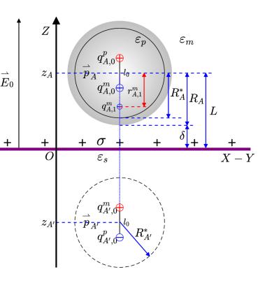
Figure 1: (color online) Schematic of electrostatic interaction between a dielectric sphere with radius $R_{A}$ and an infinite planar substrate with uniform initial charge density $\sigma$. The relative permittivities of the sphere, the planar substrate, and the medium are denoted as $\varepsilon_{p}$, $\varepsilon_{s}$, and $\varepsilon_{m}$ respectively. $L$ is the distance from the center of the dielectric sphere to the planar substrate. The hypothetical conducting sphere and the imageed one are denoted in solid and dashed circular lines, respectively. Their radii are $R_{A}^{*}$ and $R_{A^{\prime}}^{*}$, respectively. $q_{A,0}^{p}$ and $q_{A,0}^{m}$ are the initial polarized charges induced by external uniform electric field ${\mathop{E}\limits^{\rightharpoonup}}_{0}$, separated by a distance $l_{0}$. $q_{A^{\prime},0}^{m}$ and $q_{A^{\prime},0}^{p}$ are the image charges of $q_{A,0}^{m}$ and $q_{A,0}^{p}$, respectively, with respect to the planar substrate. $q_{A,1}^{m}$ is the image charge of $q_{A^{\prime},0}^{m}$ in sphere $A$. $r_{A,1}^{m}$ represents the distance between $q_{A,1}^{m}$ and the center of sphere $A$.

EFFECTIVE$-$DIPOLE APPROACH

In our previous work[47, 48], the effective$-$dipole approach (EDA), originally introduced by Chan et al.[50, 51, 52], is extended to macroscopic dielectric spheres. With this methodology, a dielectric sphere in an external uniform electric field ${\mathop{E}\limits^{\rightharpoonup}}_{0}$ can be treated as a hypothetical conducting sphere with a reduced radius ${R_{A}^{*}}^{3}=\rvert\frac{\varepsilon_{p}-\varepsilon_{m}}{\varepsilon_{p}+2\varepsilon_{m}}\rvert R_{A}^{3}$, enabling us to express Eq.(2) as:

$${\mathop{p}\limits^{\rightharpoonup}}_{A}=\frac{\varepsilon_{p}-\varepsilon_{m}}{\rvert\varepsilon_{p}-\varepsilon_{m}\rvert}4\pi\varepsilon_{m}\varepsilon_{0}{R_{A}^{*}}^{3}{\mathop{E}\limits^{\rightharpoonup}}_{0},$$ (3)

which indicates two reversed polarization conditions in a external uniform electric field. When $\varepsilon_{p}>\varepsilon_{m}$, positive polarization occurs, in which ${\mathop{p}\limits^{\rightharpoonup}}_{A}$ aligns with the direction of ${\mathop{E}\limits^{\rightharpoonup}}_{0}$. Conversely, when $\varepsilon_{p}<\varepsilon_{m}$, negative polarization happens, in which the polarization of ${\mathop{p}\limits^{\rightharpoonup}}_{A}$ is opposite to that of ${\mathop{E}\limits^{\rightharpoonup}}_{0}$.

To calculate the total polarization of sphere $A$, ${\mathop{p}\limits^{\rightharpoonup}}_{A}$, two components need to be considered: the external electric field ${\mathop{E}\limits^{\rightharpoonup}}_{0}$ and the induced electric field generated by the dipole moment ${\mathop{p}\limits^{\rightharpoonup}}_{A^{\prime}}$, which acts as the image dipole ${\mathop{p}\limits^{\rightharpoonup}}_{A}$ on the planar substrate. For the latter, it is typically assumed to be uniform within sphere $A$, with its magnitude equal to that at the center of the sphere.

$${\mathop{p}\limits^{\rightharpoonup}}_{A}=\frac{\varepsilon_{p}-\varepsilon_{m}}{\rvert\varepsilon_{p}-\varepsilon_{m}\rvert}4\pi\varepsilon_{m}\varepsilon_{0}{R_{A}^{*}}^{3}{\mathop{E}\limits^{\rightharpoonup}}_{A},$$ (4a)

$${\mathop{E}\limits^{\rightharpoonup}}_{A}={\mathop{E}\limits^{\rightharpoonup}}_{0}+\frac{2{\mathop{p}\limits^{\rightharpoonup}}_{A^{\prime}}}{4\pi\varepsilon_{m}\varepsilon_{0}(2L)^{3}},$$ (4b)

$${\mathop{p}\limits^{\rightharpoonup}}_{A^{\prime}}=-\frac{\varepsilon_{m}-\varepsilon_{s}}{\varepsilon_{m}+\varepsilon_{s}}{\mathop{p}\limits^{\rightharpoonup}}_{A},$$ (4c)

where $\frac{2{\mathop{p}\limits^{\rightharpoonup}}_{A^{\prime}}}{4\pi\varepsilon_{m}\varepsilon_{0}(2L)^{3}}$ is the electric field of the image dipole ${\mathop{p}\limits^{\rightharpoonup}}_{A^{\prime}}$ at the center of sphere $A$. A detailed derivation of Eq.(4c) can be found in A. In Eq.(4c), two interesting observations are made. Firstly, the magnitude of ${\mathop{p}\limits^{\rightharpoonup}}_{A^{\prime}}$ is smaller than that of ${\mathop{p}\limits^{\rightharpoonup}}_{A}$. Secondly, the direction of ${\mathop{p}\limits^{\rightharpoonup}}_{A^{\prime}}$ is related not only to the direction of ${\mathop{p}\limits^{\rightharpoonup}}_{A}$ but also to the difference between $\varepsilon_{m}$ and $\varepsilon_{s}$.

Combining Eqs.(4a), (4b) and (4c), we can obtain

$$\begin{split}{\mathop{p}\limits^{\rightharpoonup}}_{A}=\frac{\frac{\varepsilon_{p}-\varepsilon_{m}}{|\varepsilon_{p}-\varepsilon_{m}|}\left(4\pi\varepsilon_{m}\varepsilon_{0}{R_{A}^{*}}^{3}{\mathop{E}\limits^{\rightharpoonup}}_{0}\right)}{1+\frac{\varepsilon_{p}-\varepsilon_{m}}{|\varepsilon_{p}-\varepsilon_{m}|}\left(2\frac{\varepsilon_{m}-\varepsilon_{s}}{\varepsilon_{m}+\varepsilon_{s}}\frac{{R_{A}^{*}}^{3}}{(2L)^{3}}\right)}\end{split}.$$ (5)

Eq.5 indicates that the direction of ${\mathop{p}\limits^{\rightharpoonup}}_{A}$ is still determined by the difference in dielectric constants of the sphere and the solvent, although the presence of the substrate does influence its value.

The electrostatic interaction force $F$ between the dielectric sphere and the planar substrate can be calculated using the obtained dipole moments. When considering the colinearity of the dipole moments ${\mathop{p}\limits^{\rightharpoonup}}_{A}$ and ${\mathop{p}\limits^{\rightharpoonup}}_{A^{\prime}}$, the electrostatic interaction force can be written as follows:

$$\begin{split}F&=-\frac{3p_{A}p_{A^{\prime}}}{2\pi\varepsilon_{m}\varepsilon_{0}(2L)^{4}}\\ &=\frac{\varepsilon_{m}-\varepsilon_{s}}{\varepsilon_{m}+\varepsilon_{s}}\frac{3{p_{A}}^{2}}{2\pi\varepsilon_{m}\varepsilon_{0}(2L)^{4}}\end{split}.$$ (6)

Eq.6 indicates that the electrostatic interaction force between the sphere and the substrate is independent of the sphere^′s permittivity. Instead, it is modulated by the difference in the dielectric constants of the substrate and the solvent. When ${\varepsilon_{m}>\varepsilon_{s}}$, a repulsive interaction is obtained, whereas an attractive interaction is produced when ${\varepsilon_{m}}<{\varepsilon_{s}}$.

MULTIPLE$-$IMAGE METHOD

In the MIM framework, the initial dipole moment induced by the uniform electric field ${\mathop{E}\limits^{\rightharpoonup}}_{0}$ in sphere $A$ can be represented as a pair of effective point charges. These theoretical point charges are considered to be positioned at the center of the sphere, separated by a distance denoted as $l_{0}=10^{-4}{~{}\rm{nm}}$. In Fig.1, the pair of point charges $q_{A,0}^{p}$ and $q_{A,0}^{m}$ in sphere $A$ are illustrated as:

$$q_{A,0}^{p}=-q_{A,0}^{m}=\rvert{\mathop{p}\limits^{\rightharpoonup}}_{A,0}/{\mathop{l}\limits^{\rightharpoonup}}_{0}\rvert,$$ (7a)

$$z_{A,0}^{p}=z_{A}+{l_{0}}/2,~{}z_{A,0}^{m}=z_{A}-{l_{0}}/2,$$ (7b)

where the superscripts of $p$ and $m$ represent the positive and negative point charges, respectively.

Based on the treatment for the inductance between a sphere and a planar substrate, an image sphere ${A^{\prime}}$ is imaged at the position of $z_{A^{\prime}}=-z_{A}$ with same radius $R_{A^{\prime}}^{*}=R_{A}^{*}$. Within sphere ${A^{\prime}}$, two image charges $q_{{A^{\prime}},0}^{m}$ and $q_{{A^{\prime}},0}^{p}$ are symmetrically created at a distance $l_{0}$ from each other. For instance, considering $q_{A^{\prime},0}^{m}$, it is produced at the position $z_{{A^{\prime}},0}^{m}=-z_{A,0}^{m}$ with a charge of $q_{{A^{\prime}},0}^{m}=\frac{\varepsilon_{m}-\varepsilon_{s}}{\varepsilon_{m}+\varepsilon_{s}}q_{A,0}^{m}$. This results in an electrostatic interaction force between the dielectric sphere $A$ and the planar substrate that is analogous to that between the reduced sphere and the image sphere ${A^{\prime}}$. The MIM is then employed to calculate the polarization of sphere $A$ due to the image charges in sphere ${A^{\prime}}$. Taking the image charge $q_{A^{\prime},0}^{m}$ as an example, its image charge $q_{A,1}^{m}$ in sphere $A$ is at a distance of $r_{A,1}^{m}={R_{A}^{*}}^{2}/(z_{A}-z_{{A^{\prime}},0}^{m})$ from the sphere center, with a charge of $q_{{A},1}^{m}=-\frac{\varepsilon_{p}-\varepsilon_{m}}{\rvert\varepsilon_{p}-\varepsilon_{m}\rvert}R_{A}^{*}q_{{A^{\prime}},0}^{m}/(z_{A}-z_{{A^{\prime}},0}^{m})$. Similar procedures are repeated for $q_{A^{\prime},0}^{p}$ and $q_{A,1}^{p}$ is generated in sphere $A$. Then the first group of image charges in sphere $A$ is established after the first iteration of MIM. Next, the MIM iteration progresses, generating successive groups of image charges in sequence. The magnitudes and positions of these image charges are determined based on the iteration step,

$$q^{\lambda}_{{A^{\prime}},n}=\frac{\varepsilon_{m}-\varepsilon_{s}}{\varepsilon_{m}+\varepsilon_{s}}q_{A,n}^{\lambda},$$ (8a)

$$z_{{A^{\prime}},n}^{\lambda}=-z_{A,n}^{\lambda},$$ (8b)

$$q^{\lambda}_{A,n+1}=-\frac{\varepsilon_{p}-\varepsilon_{m}}{\rvert\varepsilon_{p}-\varepsilon_{m}\rvert}R_{A}^{*}q_{{A^{\prime}},n}^{\lambda}/(z_{A}-z_{{A^{\prime}},n}^{\lambda}),$$ (8c)

$$r_{A,n+1}^{\lambda}={R_{A}^{*}}^{2}/(z_{A}-z_{{A^{\prime}},n}^{\lambda}),$$ (8d)

$$z^{\lambda}_{A,n+1}=z_{A}-r_{A,n+1}^{\lambda},$$ (8e)

where $\lambda=m,p$ and $n=0,1,\cdots$.

When a sufficient iteration number of the MIM is reached, it becomes necessary to introduce the first compensation point charge, denoted as $q^{c_{0}}_{A,0}$, located at the center of sphere $A$. The specific compensation charge is essential for preserving the conservation of charge within the sphere,

$$q^{c_{0}}_{A,0}=-\sum_{n=0}^{N}q^{m}_{A,n}-\sum_{n=0}^{N}q^{p}_{A,n}.$$ (9)

A similar process of image iteration is also required for the compensation charge $q^{c_{0}}_{A,0}$. This results in the generation of a series of corresponding image charges $q^{c_{0}}_{A,n^{\prime}}$ and $q^{c_{0}}_{{A^{\prime}},n^{\prime}}$. Subsequently, the compensation point charges are once again introduced at the center of the sphere. These compensation charges, along with their corresponding series of image charges, satisfy the following relationships:

$$q^{c_{1}}_{A,0}=-\sum_{n^{\prime}=1}^{N^{\prime}}{q^{c_{0}}_{A,n^{\prime}}},$$ (10)

where $n^{\prime}$ and $N^{\prime}$ are the index and the total number of iteration for the compensation charges. As the iteration process continues, the compensation charge sequences, denoted as $q^{c_{2}}_{A,0},q^{c_{3}}_{A,0}...$, are generated. It has been observed that these sequences tend to approach zero, indicating that the compensation charges become increasingly insignificant as the iterations advance.

Once the polarization, image charges, and compensation charges have been determined, the spatial potential $U^{q}$ outside sphere $A$ and above the planar substrate can be precisely calculated. Additionally, the electrostatic interaction force $F_{A}$ acting on sphere $A$ from the substrate can be calculated using the acquired charges.

$$\begin{array}[]{ll}U^{q}=\frac{1}{4{\pi}\varepsilon_{m}{\varepsilon_{0}}}\sum\limits_{i=A,{A^{\prime}}}\sum\limits_{\lambda=p,m,\atop c_{\tiny 0},c_{\tiny 1},c_{\tiny 2}...}\sum\limits_{n=0}^{N}\frac{q_{i,n}^{\lambda}}{[(x_{i,n}^{\lambda}-x)^{2}+(y_{i,n}^{\lambda}-y)^{2}+(z_{i,n}^{\lambda}-z)^{2}]^{1/2}}\end{array},$$ (11)

$$\begin{array}[]{ll}F_{A}=\frac{1}{4{\pi}{\varepsilon_{m}}{\varepsilon_{0}}}\sum\limits_{\lambda_{{}_{A}},\lambda_{{}_{A^{\prime}}}=p,m,\atop c_{0},c_{1},c_{2}...}\sum\limits_{n_{{}_{A}},n_{{}_{A^{\prime}}}=0}^{N}\frac{q_{A,n_{A}}^{\lambda_{A}}q_{{A^{\prime}},n_{A^{\prime}}}^{\lambda_{A^{\prime}}}}{(x_{A,n_{A}}^{\lambda_{A}}-x_{{A^{\prime}},n_{A^{\prime}}}^{\lambda_{A^{\prime}}})^{2}+(y_{A,n_{A}}^{\lambda_{A}}-y_{{A^{\prime}},n_{A^{\prime}}}^{\lambda_{A^{\prime}}})^{2}+(z_{A,n_{A}}^{\lambda_{A}}-z_{{A^{\prime}},n_{A^{\prime}}}^{\lambda_{A^{\prime}}})^{2}}\end{array},$$ (12)

where $x_{i,n}^{\lambda}=y_{i,n}^{\lambda}=0$. In all calculations, a total of $N=400$ iterations are employed to ensure numerical convergence. Additionally, it is crucial to acknowledge that the particles are electrically neutral, and therefore, it does not undergo any net force in an external uniform field ${\mathop{E}\limits^{\rightharpoonup}}_{0}$.

RESULTS AND DISCUSSIONS

Fig.2 shows the electrostatic interaction force between a neutral dielectric sphere and a dielectric planar substrate using the MIM and the EDA. In accordance with parameters from previous experiments[27], the sphere is made of alumina with a relative permittivity $\varepsilon_{p}=9.9$. The planar substrate, which features a charged nanodiamond surface with a net charge density of $\sigma=1\rm~{}e\cdot nm^{-2}$, also has a relative permittivity of $\varepsilon_{s}=5.3$. Additionally, in Fig.2(a), the medium is an insulating fluorocarbon solution with a relative permittivity of $\varepsilon_{m}=1.86$. Notably, in Fig.2(b), an alternative configuration is presented, utilizing acetone as the medium with a higher dielectric constant of $\varepsilon_{m}=20.0$[28]. In this study, the selected sphere radius is set at $10~{}{\rm nm}$, a common size for nanoscale particles.

The calculations also involve the use of the simple$-$dipole method (SDM), which considers only the charges $q_{A,0}^{\lambda}$ of the sphere and $q_{{A^{\prime}},0}^{\lambda}$ of the substrate. The results obtained from all three methods (MIM, EDA, and SDM) exhibit agreement for large separations $\delta$. However, for small separations, the absolute values of the calculated forces obtained from the MIM are greater than those from the EDA and SDM. This discrepancy becomes more pronounced as the separation decreases. The underlying reason for this difference lies in the distinct approaches employed by these methods. In the SDM, the multiple mutual polarizations between the sphere and the substrate are not considered. In the EDA, the polarized dipole moment is positioned at the center of the sphere $A$, whereas in the MIM, the image charges of the dipole moment are dispersed away from the center of the sphere. This implies that the MIM approach captures the intricate interactions more accurately, thus providing a more comprehensive understanding of the system. The subsequent analyses are conducted using the MIM.

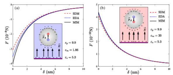
Figure 2: (color online) Dependence of the electrostatic interaction force $F$ between a neutral dielectric sphere and a planar substrate. The radius of the sphere $A$ is $R_{A}={10~{}\rm nm}$ and its relative permittivity is set to $\varepsilon_{p}=9.9$. The charge density of the planar substrate is $\sigma=1\rm~{}e\cdot nm^{-2}$ and its relative permittivity is $\varepsilon_{s}=5.3$. The relative permittivities of the solvent are (a) $\varepsilon_{m}=1.86$ and (b) $\varepsilon_{m}=20.0$. Solid, dotted and dashed lines represent the results using MIM, EDA, and SDM, respectively. The insets provide a schematic illustration of the multiple dipole moment.

In Fig.2, negative and positive values of $F$ represent attractive and repulsive interaction forces, respectively. The relative permittivities of the sphere and the substrate are fixed at ${\varepsilon_{p}}=9.9$ and $5.3$, respectively. The results obtained from all three methods indicate an attractive interaction in a weakly polarizable solvent, $\varepsilon_{m}=1.86$, shown in Fig.2(a) and a repulsive force in a strongly polarizable solvent, $\varepsilon_{m}=20$ shown in Fig.2(b). This reversed polarization is in agreement with the predictions of $EDA$ and the previous work of dielectrophoresis (DEP)[28, 20]. When the relative permittivity of the sphere is higher than that of the solvent, $\varepsilon_{p}>\varepsilon_{m}$, more polarization charges accumulate at the sphere side, schematically indicated by ${\mathop{p}\limits^{\rightharpoonup}}_{A}$ in Fig.2(a). The direction of ${\mathop{p}\limits^{\rightharpoonup}}_{A}$ is aligned in the positive direction of the $z-$axis, which is consistent with the result of Eq.3. On the contrary, when the solvent has a higher relative permittivity $\varepsilon_{m}>\varepsilon_{p}$, it becomes more polarizable than the sphere. The reversed polarization charges appear on the solvent interface. In this case, the resultant dipole moment is shown in the inset of Fig.2(b), which is in the negative direction of the $z-$axis.

Figure 3: (color online) Spatial distribution of electric isopotential $U^{q}$ of the polarized charges. The same parameters are used as in Fig.2. The separation gap is $\delta=5\rm nm$. The relative permittivities of the solvent are (a) $\varepsilon_{m}=1.86$ and (b) $\varepsilon_{m}=20.0$, respectively.

The above results have shown that the attractive and repulsive interaction between a neutral dielectric sphere and a planar dielectric substrate can be entirely reversed by adjusting the dielectric constant of the solvent. It is of significant importance to discover the influence of polarized charges on spatial distribution of electric isopotential $U^{q}$. Fig.3 plots the $U^{q}$ outside of the sphere calculated by the MIM with zero electric potential at infinity. Fig.3$(\rm a_{1})$ plots the $U^{q}$ generated solely by the polarized charges on sphere $A$, with same parameters as shown in Fig.2(a). The initial uniform electric field is expected to be disrupted around sphere $A$. An axial symmetry with the same $U^{q}$ in the $x$ direction is observed due to the identical nature of the sphere. In the $z$ direction, an almost axial symmetry with reversed $U^{q}$ is also observed though a tiny difference exists. Positive and negative $U^{q}$ appear around the upper and lower regions of sphere $A$, respectively. This is equivalent to a dipole moment aligned with the same direction of ${\mathop{E}\limits^{\rightharpoonup}}_{0}$, consistent with the result of Eq.5. In Fig.3$(\rm a_{2})$, the positive $U^{q}$ generated by the polarized charges on the substrate indicates that the polarized charges on the substrate are positive. In the other words, it is actually calculated by the dipole moment at sphere ${A^{\prime}}$. This positive $U^{q}$ above the substrate implies that the direction of ${\mathop{P}\limits^{\rightharpoonup}}_{A^{\prime}}$ aligns with the direction of ${\mathop{E}\limits^{\rightharpoonup}}_{0}$. Furthermore, the nonuniform distribution of $U^{q}$ indicates the generation of a nonuniform electric field, with stronger and weaker electric fields occurring at the lower and upper regions of sphere $A$. This gradient electric field directly results in the occurrence of positive dielectrophoresis. Additionally, it leads to an attractive electrostatic interaction between sphere $A$ and the substrate. Fig.3$(\rm a_{3})$ plots the combined $U^{q}$ of the polarized charges on the sphere $A$ and the substrate, as shown in Fig.3$(\rm a_{1})$ and Fig.3$(\rm a_{2})$. It is evident that the former significantly dominates the distribution of $U^{q}$, with positive and negative $U^{q}$ still appearing around the upper and lower parts regions of sphere $A$, respectively.

We also plot the distribution of $U^{q}$ for the case of Fig.2(b) as shown in Fig.3. The solvent has a large relative permittivity, $\varepsilon_{m}=20$. All similar panels in Fig.3 exhibit analogous properties of $U^{q}$. In the $x$ direction, the identical nature of sphere results in complete symmetry, as shown in Fig.3($\rm b_{1}$). Conversely, in the $z$ direction, the dipole moment at sphere $A$ is reversed as expected from Eq.5, producing positive and negative $U^{q}$ at the lower and upper regions of sphere $A$, respectively. As predicted by Eq.5, positive $U^{q}$ is expected to appear at the region above the substrate, indicating a repulsive electrostatic interaction between sphere $A$ and the substrate. Likewise, $U^{q}$ is predominantly influenced by the polarization charges at the sphere $A$.

In order to systematically investigate the influence of relative permittivity ($\varepsilon_{p}$, $\varepsilon_{m}$ and $\varepsilon_{s}$) on the interaction force, the numerical results are summarized in Table 1, as predicted by Eq.(3), Eq.(4c) and Eq.(5). As indicated by Eq.(3), for ${\varepsilon_{p}}>{\varepsilon_{m}}$, positive polarization occurs for sphere $A$. Conversely, negative polarization of sphere $A$ arises when ${\varepsilon_{p}}<{\varepsilon_{m}}$. This leads to the generation of positive and negative dielectrophoresis depending on the polarization direction of sphere $A$. In Eq.(4c), the polarization of the image sphere ${A^{\prime}}$ is determined by the difference between ${\varepsilon_{s}}$ and ${\varepsilon_{m}}$ along with the polarization state of the sphere $A$. However, according to Eq.(5), the electrostatic interaction force between sphere $A$ and the substrate solely depends on the difference between ${\varepsilon_{s}}$ and ${\varepsilon_{m}}$. The simulation results obtained using the MIM validate the theoretical predictions of the EDA. Taking case $1$ for example, when ${\varepsilon_{p}}>{\varepsilon_{s}}>{\varepsilon_{m}}$, it corresponds to the results shown in Fig.2(a) and Fig.3($\rm a$). In this scenario, sphere $A$ exhibits positive polarization, resulting in positive dielectrophoresis. As a consequence, positive polarized charges accumulate on the surface of the substrate, leading to an attractive electrostatic interaction force between sphere $A$ and the substrate.

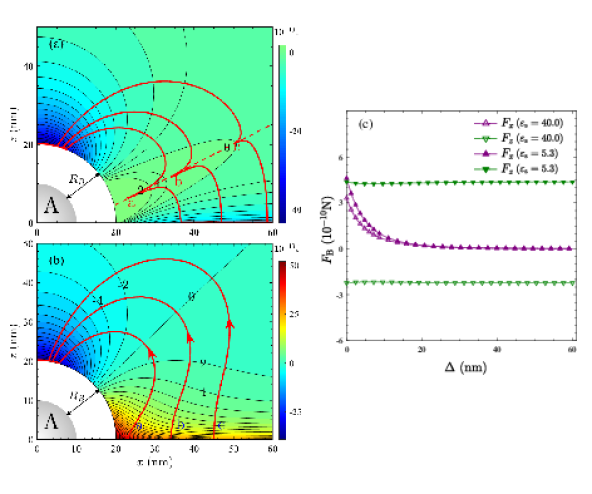
Figure 4: (color online) Spatial distribution of mutual$-$energy of sphere $B$ with sphere $A$ and the substrate in the medium with $\varepsilon_{m}=20.0$. Sphere $A$ is fixed on the substrate with a separation distance of $\delta=0~{}\rm nm$, and the substrate is located at $z=-10~{}\rm nm$. The relative permittivities of the substrate are (a) $\varepsilon_{s}=40.0$ and (b) $\varepsilon_{s}=5.3$, respectively. The solid red lines represent gradient lines, and the width of the white sector corresponds to the radius of sphere $B$. (c) The electrostatic force $F_{B}$ as a function of the gap $\Delta$ between spheres $A$ and $B$. Upward triangles and downward triangles denote $F_{x}$ and $F_{z}$, respectively. Open and solid symbols represent the results of (a) $\varepsilon_{s}=40.0$ and (b) $\varepsilon_{s}=5.3$, respectively.

Since the electrostatic interaction force between sphere $A$ and the substrate is directly modulated by the difference of the relative permittivity between the solvent and the substrate, it is interesting to explore how the relative permittivity of the substrate influences the self$-$assembly of the particles. Let us consider the case of two identical particles $A$ and $B$. Particle $A$ is fixed on the substrate, and particle $B$ is movable. The electrostatic interaction between the particles $A$ and $B$ is calculated using the MIM[47, 48]. The relative permittivities of the substrate, the solvent and the particle are set to $\varepsilon_{s}=40.0$, $\varepsilon_{m}=20.0$ and $\varepsilon_{p}=9.9$, corresponding to the case $6$ in Table 1. Under these conditions, the electrostatic interaction force between the substrate and each particle is attractive. Fig.4(a) plots the distribution of the electrostatic energy for particle $A$, particle $B$ and the substrate, while ignoring any changes of self$-$energy due to the position shift of polarization charges in each particle and the substrate. The three red lines represent typical gradient lines. The direction of the tangent at any point on a gradient line indicates the electrostatic interaction force of particle $B$ from particle $A$ and the substrate. It is evident that lower energy levels occur on the upper side of particle $A$ and at the surface of the substrate. A ridge line for the electrostatic energy, denoted by the dashed line, is clearly observed, dividing the space into two regions. This ridge line does not intersect with the gradient lines. If particle $B$ falls exactly on the ridge line, such as the points ${\rm a}$, $b$ or $\rm c$, the resultant force on particle $B$ will push it away along the dashed line. If particle $B$ deviates slightly from the ridge line, it will move toward the upper side of particle $A$ or the substrate, respectively. When the relative permittivity of the substrate is $\varepsilon_{s}=5.3$, the electrostatic energy and the corresponding gradient lines are also plotted in Fig.4(b). Lower energy levels occur at the upper side of particle $A$, while the higher energy levels appear at the surface of the substrate, respectively. Notably, no ridge line appears. These characteristics indicate that particles $A$ and $B$ will be aligned along a line in the direction of ${\mathop{E}\limits^{\rightharpoonup}}_{0}$.

In Fig.4(c), the electrostatic force of particle $B$ received from particle $A$ and the substrate is plotted when particle $B$ is located at the surface of the substrate. It is noticeable that $F_{x}$ keeps positive, indicating a repulsive force, regardless of the relative permittivity of the substrate. This consistent behavior can be attributed to the similar nature of particles of $A$ and $B$, which result in parallel polarizations. However, for large $\varepsilon_{s}=40$ and small $\varepsilon_{s}=5.3$, we observe negative and positive values for $F_{z}$, indicating attractive and repulsive forces, respectively. These observations align with the results illustrated in Figs.4(a) and 4(b).

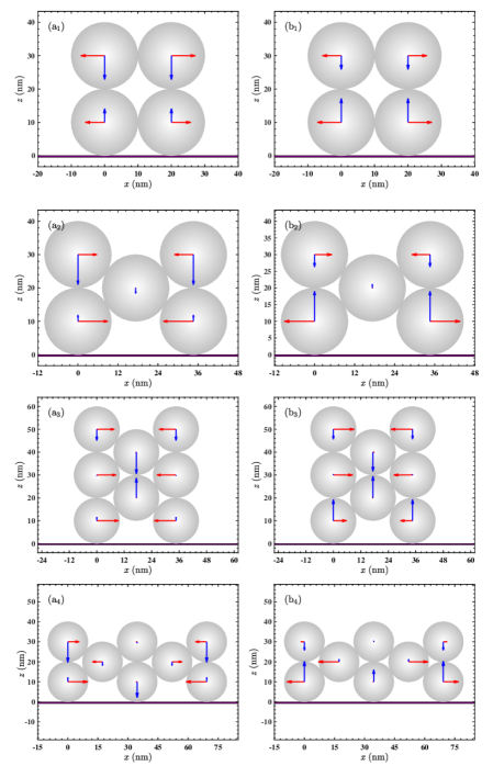
Figure 5: (color online) The electrostatic forces experienced by spheres with different numbers and structures with (a) $\varepsilon_{s}=40.0$ and (b) $\varepsilon_{s}=5.3$. The vertical axis (denoted as z) is indicated by blue vectors, and the horizontal axis (denoted as x) is indicated by red vectors. Within different subfigures, the lengths of vectors in different colors are adaptive in order to more effectively demonstrate and comprehend electrostatic forces.

When more particles are introduced, it becomes essential to observe the stable geometrical structure that the particles will aggregate under the influence of an external electric field. Fig.5 employs the same parameters as Fig.4 with the dielectric constants set at $\varepsilon_{s}=40.0$ and $\varepsilon_{s}=5.3$ for the left and right panels of Fig.5, respectively. Two distinct geometrical structures are examined: the square structure and the hexagonal structure. In Fig.5, the length of the arrows represents the magnitude of the electric force in the $x$ and $z$ directions. Generally, the characteristics of the electrostatic force between the substrate and the cluster exhibit similarities to those between a single particle and the substrate in the $z$ direction. When $\varepsilon_{s}=40.0$, the resultant electrostatic force between the cluster and the substrate is attractive, while it becomes repulsive when $\varepsilon_{s}=5.3$. Additionally, the electrostatic force remains consistently attractive among the particles, suggesting that the chain-like structure is stable for the particles in the $z$ direction. However, the stability of particle aggregation in the $x$ direction is closely associated with the geometrical structure. For instance, in Fig.4$\rm(a_{1})$ and Fig.4$\rm(b_{1})$, the square arrangement of particles is unstable because the electrostatic force always points outward from the interior of the cluster in the $x$ direction. Conversely, the hexagonal structure exhibits stability in the $x$ direction since the peripheral particles experience inward electrostatic forces for $\varepsilon_{s}=40$, as depicted in Fig.4$\rm(a_{2})$. In contrast, when $\varepsilon_{s}=5.3$, the particles tend to separate in the $x$ direction due to outward electrostatic forces. Upon introducing an additional layer of particles in the $z$ direction, the hexagonal structure proves to be stable for both both $\varepsilon_{s}=40$ and $\varepsilon_{s}=5.3$, as shown in Fig.4$\rm(a_{3})$ and Fig.4$\rm(b_{3})$. However, adding an extra layer of particles in the $x$ direction results in stability within the hexagonal structure for $\varepsilon_{s}=40$, as shown in Fig.4$\rm(a_{4})$. On the other hand, for $\varepsilon_{s}=5.3$, the hexagonal structure becomes unstable as the electrostatic force on the particles points outward, as depicted Fig.4$\rm(b_{4})$.

CONCLUSIONS

In conclusion, we conducted numerical investigations of the electrostatic interaction forces between dielectric spherical particles and a uniformly charged substrate using the EDA and the MIM. By applying the CM relation, an equivalent conducting sphere with a smaller radius and a polarized dipole moment was introduced in a uniform electrostatic field. Image charges were symmetrically placed in the substrate depending on the dielectric constants of the solvent medium and the substrate. In the EDA, an analytical formula was derived, while the computation iterations were established in the MIM for analyzing the electrostatic interactions thoroughly.

Both the EDA and the MIM results initially revealed the attractive and repulsive electrostatic interactions between the neutral particle and the substrate for $\varepsilon_{s}>\varepsilon_{m}$ and $\varepsilon_{s}<\varepsilon_{m}$, respectively. The analysis of the distribution of electrostatic potential indicated that the variations of the dielectric constants of the particle and the solvent medium can lead to transitions between positive and negative polarizations of the particle. The polarized charges of the substrate consistently created a nonuniform local electrostatic potential around the particle, resulting in both attractive and repulsive electrostatic interactions. Generally, positive polarization occurs when $\varepsilon_{p}/\varepsilon_{m}>1$, whereas negative polarization arises for $\varepsilon_{p}/\varepsilon_{m}<1$. Furthermore, attractive and repulsive electrostatic interactions are observed for $\varepsilon_{s}/\varepsilon_{m}>1$ and $\varepsilon_{s}/\varepsilon_{m}<1$, respectively. Subsequent analysis of the electrostatic potential and its gradient for a system with two particles indicates that the electrostatic field of the substrate arranges particles in a line. Notably, higher dielectric constants of the substrate tend to cause neutral particles to absorb to the substrate, whereas lower dielectric constants push neutral particles away from the substrate. When multiple particles are considered, they exhibit a preference for forming a hexagonal structure rather than a square one. These findings offer valuable insights into the electrostatic manipulation of the design and fabrication of advanced materials.

Appendix A THE IMAGE OF A POINT CHARGE

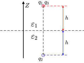
Figure 1: (color online) Schematic of the image method for a point charge in proximity to the interface of two dielectrics, where the dielectric constants are $\varepsilon_{1}$ and $\varepsilon_{2}$, respectively. $h$ is the distance from the point charge to the interface.

In the computation of electric potential within either dielectric $1$ or $2$, we employ image charges situated in the alternate dielectric medium as a substitute for polarization charges at the interface. Correspondingly, we consider the entire space as a homogeneous medium filled with a dielectric constant of $\varepsilon_{1}$ for dielectric $1$, and $\varepsilon_{2}$ for dielectric $2$, as shown in Fig. 1.

The potential at any point in the space can be expressed as

$$\varphi\left(x,y,z\right)=\begin{cases}\frac{1}{4\pi\varepsilon_{1}}\left[\frac{q_{1}}{\sqrt{x^{2}+y^{2}+\left(z-h\right)^{2}}}+\frac{q_{2}}{\sqrt{x^{2}+y^{2}+\left(z+h\right)^{2}}}\right],&\text{if }z\geq 0\\ \frac{1}{4\pi\varepsilon_{2}}\frac{q_{1}+q_{3}}{\sqrt{x^{2}+y^{2}+\left(z-h\right)^{2}}}.&\text{if }z\leq 0\end{cases}$$ (13)

According to the boundary conditions:

$$\varphi_{1}|_{z=0}=\varphi_{2}|_{z=0},$$ (14a)

$$\varepsilon_{1}\frac{\partial\varphi_{1}}{\partial z}\Bigr{|}_{z=0}=\varepsilon_{2}\frac{\partial\varphi_{2}}{\partial z}\Bigr{|}_{z=0},$$ (14b)

we can obtain

$$\frac{1}{\varepsilon_{1}}\left(q_{1}+q_{2}\right)=\frac{1}{\varepsilon_{1}}\left(q_{1}+q_{3}\right),$$ (15a)

$$q_{1}-q_{2}=q_{1}+q_{3}.$$ (15b)

Upon simplification of Eqs.(15a) and (15b), Eqs.(16a) and (16b) are derived,

$$q_{2}=\frac{\varepsilon_{1}-\varepsilon_{2}}{\varepsilon_{1}+\varepsilon_{2}}q_{1},$$ (16a)

$$q_{3}=-\frac{\varepsilon_{1}-\varepsilon_{2}}{\varepsilon_{1}+\varepsilon_{2}}q_{1}.$$ (16b)

For the image of an electric dipole near a boundary interface, both magnitude and direction need to be considered. Specifically, when the direction of the original dipole is perpendicular to the interface, the dipole moment of the image dipole, denoted as ${\mathop{p}\limits^{\rightharpoonup}}_{B}$, is proportional to the original dipole moment, denoted as ${\mathop{p}\limits^{\rightharpoonup}}_{A}$. The magnitude and direction can be determined by the following equation:

$$\begin{split}{\mathop{p}\limits^{\rightharpoonup}}_{B}=-\frac{\varepsilon_{1}-\varepsilon_{2}}{\varepsilon_{1}+\varepsilon_{2}}{\mathop{p}\limits^{\rightharpoonup}}_{A}\end{split}.$$ (17)

References

- [1] Huang, T. C., Zhou, X. P., Ren, C. L., Zhan, P. and Ma, Y. Q. Selfassembled binary photonic crystals under the active confinement and their light trapping. Langmuir 36, 42244230 (2020).
- [2] Levay, S. et al. Frustrated packing in a granular system under geometrical confinement. Soft Matter 14, 396404 (2018).
- [3] Liang, R. et al. Assembly of PolymerTethered Gold Nanoparticles under Cylindrical Confinement. ACS Macro Lett. 3, 486490 (2014).
- [4] Bishop, K. J. M., Wilmer, C. E., Soh, S. and Grzybowski, B. A. Nanoscale forces and their uses in selfassembly. Small 5, 16001630 (2009).
- [5] Tang, J. et al. Tubegraftsheet nanoobjects created by a stepwise selfassembly of polymerpolyoxometalate hybrids. Langmuir 32, 460467 (2016).
- [6] Walker, D. A., Kowalczyk, B., De La Cruz, M. O. and Grzybowski, B. A. Electrostatics at the nanoscale. Nanoscale 3, 13161344 (2011).
- [7] Rossi, E., RuizLopez, J. A., VázquezQuesada, A. and Ellero, M. Dynamics and rheology of a suspension of superparamagnetic chains under the combined effect of a shear flow and a rotating magnetic field. Soft Matter 17, 60066019 (2021).
- [8] Mann, N. Chain formation in a twodimensional system of hard spheres with a shortrange anisotropic interaction. Physical Review E 100, 042118 (2019).
- [9] SpataforaSalazar, A., Lobmeyer, D. M., Cunha, L. H. P., Joshi, K. and Biswal, S. L. Hierarchical assemblies of superparamagnetic colloids in timevarying magnetic fields. Soft Matter 17, 11201155 (2021).
- [10] RuizLópez, J. A., Wang, Z. W., HidalgoAlvarez, R. and De Vicente, J. Simulations of model magnetorheological fluids in squeeze flow mode. Journal of Rheology 61, 871881 (2017).
- [11] Domingos, C., De Freitas, E. A. and Ferreira, W. P. Steady states of nonaxial dipolar rods driven by rotating fields. Soft Matter 16, 12011210 (2020).
- [12] Yakovlev, E. V. et al. 2D colloids in rotating electric fields: A laboratory of strong tunable threebody interactions. Journal of Colloid and Interface Science 608, 564574 (2022).
- [13] Sherman, Z. M., Ghosh, D. and Swan, J. W. Fielddirected selfassembly of mutually polarizable nanoparticles. Langmuir 34, 71177134 (2018).
- [14] Van Blaaderen, A. et al. Manipulating the self assembly of colloids in electric fields. European Physical Journal Special Topics 222, 28952909 (2013).
- [15] Almudallal, A. M. and SaikaVoivod, I. Simulation of a twodimensional model for colloids in a uniaxial electric field. Physical Review E 84, 011402 (2011).
- [16] Cho, J. K., Meng, Z., Lyon, L. A. and Breedveld, V. Tunable attractive and repulsive interactions between pHresponsive microgels. Soft Matter 5, 3599 (2009).
- [17] Dempster, J. M. and Olvera De La Cruz, M. Aggregation of Heterogeneously Charged Colloids. ACS Nano 10, 59095915 (2016).
- [18] Colla, T. et al. SelfAssembly of Ionic Microgels Driven by an Alternating Electric Field: Theory, Simulations, and Experiments. ACS Nano 12, 43214337 (2018).
- [19] Yoon, C.M., Jang, Y., Noh, J., Kim, J. and Jang, J. Smart Fluid System Dually Responsive to Light and Electric Fields: An Electrophotorheological Fluid. ACS Nano 11, 97899801 (2017).
- [20] Cetin, B. and Li, D. Dielectrophoresis in microfluidics technology. Electrophoresis 32, 24102427 (2011).
- [21] Helal, A., Qian, B., McKinley, G. H. and Hosoi, A. E. Yield hardening of electrorheological fluids in channel flow. Physical Review Applied 5, 064011 (2016).
- [22] Fertig, D., Boda, D. and Szalai, I. Induced permittivity increment of electrorheological fluids in an applied electric field in association with chain formation: A brownian dynamics simulation study. Physical Review E 103, 062608 (2021).
- [23] Mohammad, T., Bharti, V., Kumar, V., Mudgal, S. and Dutta, V. Spray coated europium doped PEDOT:PSS anode buffer layer for organic solar cell: The role of electric field during deposition. Organic Electronics 66, 242248 (2019).
- [24] Huo, X. and Yossifon, G. Significant enhancement of the electrorheological effect by nonstraight electrode geometry. Soft Matter 15, 64556460 (2019).
- [25] Woehl, T. J., Heatley, K. L., Dutcher, C. S., Talken, N. H. and Ristenpart, W. D. ElectrolyteDependent Aggregation of Colloidal Particles near Electrodes in Oscillatory Electric Fields. Langmuir 30, 48874894 (2014).
- [26] Suehiro, S. et al. Electrospray deposition of 200 oriented regularassembly BaTiO 3 nanocrystal films under an electric field. Langmuir 35, 54965500 (2019).
- [27] Verveniotis, E., Kromka, A., Ledinský, M., Čermák, J. and Rezek, B. Guided assembly of nanoparticles on electrostatically charged nanocrystalline diamond thin films. Nanoscale Res Lett 6, 144 (2011).
- [28] Lindgren, E. B. et al. Electrostatic selfassembly: Understanding the significance of the solvent. Journal of Chemical Theory and Computation 14, 905915 (2018).
- [29] Liu, S., Kurth, D. G., Bredenkötter, B. and Volkmer, D. The structure of selfassembled multilayers with polyoxometalate nanoclusters. Journal of the American Chemical Society 124, 1227912287 (2002).
- [30] Lee, H. et al. Threedimensional assembly of nanoparticles from charged aerosols. Nano Letters 11, 119124 (2011).
- [31] Cho, H., MorenoHernandez, I. A., Jamali, V., Oh, M. H. and Alivisatos, A. P. In situ quantification of interactions between charged nanorods in a predefined potential energy landscape. Nano Letters 21, 628633 (2021).
- [32] Rupp, B., TorresDiaz, I., Hua, X. and Bevan, M. A. Measurement of anisotropic particle interactions with nonuniform ac electric fields. Langmuir 34, 24972504 (2018).
- [33] Mittal, M., Lele, P. P., Kaler, E. W. and Furst, E. M. Polarization and interactions of colloidal spheres in ac electric fields. The Journal of Chemical Physics 129, 064513 (2008).
- [34] Chiu, C. W. and Ducker, W. A. Direct measurement of fieldinduced polarization forces between spheres in air. Langmuir 30, 140148 (2014).
- [35] Gao, X., Wang, Q., Li, C. X., Hu, L. and Sun, G. Electric interaction between two identical conducting spheres in a uniform electric field. Acta Physica Polonica A 128, 289294 (2015).
- [36] Wang, Z. Y., Shen, R., Liu, X. J., Lu, K. Q. and Wen, W. J. Experimental investigation for fieldinduced interaction force of two spheres. Journal of Applied Physics 94, 7832 (2003).
- [37] Gao, X., Wang, Q., Sun, G., Li, C. and Hu, L. Two identical conducting spheres with same potential in a uniform electric field. Journal of Electrostatics 77, 8893 (2015).
- [38] Bichoutskaia, E., Boatwright, A. L., Khachatourian, A. and Stace, A. J. Electrostatic analysis of the interactions between charged particles of dielectric materials. The Journal of Chemical Physics 133, 024105 (2010).
- [39] Khachatourian, A., Chan, H. K., Stace, A. J. and Bichoutskaia, E. Electrostatic force between a charged sphere and a planar surface: A general solution for dielectric materials. The Journal of Chemical Physics 140, 074107 (2014).
- [40] Lindgren, E. B., Chan, H. K., Stace, A. J. and Besley, E. Progress in the theory of electrostatic interactions between charged particles. Physical Chemistry Chemical Physics 18, 58835895 (2016).
- [41] Lindgren, E. B. et al. An integral equation approach to calculate electrostatic interactions in manybody dielectric systems. Journal of Computational Physics 371, 712731 (2018).
- [42] Hassan, M. et al. Manipulating interactions between dielectric particles with electric fields: A general electrostatic manybody framework. Journal of Chemical Theory and Computation 18, 62816296 (2022).
- [43] Meyer, M. Numerical and analytical verifications of the electrostatic attraction between two likecharged conducting spheres. Journal of Electrostatics 77, 153156 (2015).
- [44] Tao, R. and Sim, H. K. Finiteelement analysis of electrostatic interactions in electrorheological fluids. Physical Review E 52, 2727 (1995).
- [45] Davis, L. C. Polarization forces and conductivity effects in electrorheological fluids. Journal of Applied Physics 72, 13341340 (1992).
- [46] Gao, X., Hu, L. and Sun, G. Multiple Image Method for the Two Conductor Spheres in a Uniform Electrostatic Field. Commun. Theor. Phys. 57, 10661070 (2012).
- [47] Li, X., Gao, X., Sun, G. and Huang, D. Giant electrostatic interaction between two neutral conducting spheres in a uniform electric field: A theoretical study via the multipleimage method. Mod. Phys. Lett. B 36, 2250085 (2022).
- [48] Li, X., Li, C., Gao, X. and Huang, D. Likecharge attraction between two identical dielectric spheres in a uniform electric field: a theoretical study via a multipleimage method and an effectivedipole approach. J. Mater. Chem. A 12, 68966905 (2024).
- [49] Guo, S. H. Electrodynamics. Higher Education Press, 2008, 4951.
- [50] Chan, H. K. A theory for likecharge attraction of polarizable ions. Journal of Electrostatics 105, 103435 (2020).
- [51] Guo, C. and Chan, H. K. Mechanisms of likecharge attraction in threebody systems. Journal of Electrostatics 122, 103793 (2023).
- [52] Zhang, X., Chen, W., Wang, M. and Chan, H. K. Mechanisms of likecharge attraction in manybody systems. Journal of Electrostatics 126, 103859 (2023).