Feature Responsiveness Scores:
Model-Agnostic Explanations for Recourse

Abstract

Machine learning models are often used to automate or support decisions in applications such as lending and hiring. In such settings, consumer protection rules mandate that we provide a list of “principal reasons” to consumers who receive adverse decisions. In practice, lenders and employers identify principal reasons by returning the top-scoring features from a feature attribution method. In this work, we study how such practices align with one of the underlying goals of consumer protection – recourse – i.e., educating individuals on how they can attain a desired outcome. We show that standard attribution methods can mislead individuals by highlighting reasons without recourse – i.e., by presenting consumers with features that cannot be changed to achieve recourse. We propose to address these issues by scoring features on the basis of responsiveness – i.e., the probability that an individual can attain a desired outcome by changing a specific feature. We develop efficient methods to compute responsiveness scores for any model and any dataset under complex actionability constraints. We present an extensive empirical study on the responsiveness of explanations in lending, and demonstrate how responsiveness scores can be used to construct feature-highlighting explanations that lead to recourse and to mitigate harm by flagging instances with fixed predictions.

Keywords: Explainability, Recourse, Actionability, Feature Attribution, Consumer Finance, Consumer Protection

1 Introduction

Machine learning models are now routinely used to automate or support decisions about people in domains such as employment [9, 46], consumer finance [27], and public services [62, 18, 25]. In such applications, explanations are often seen as an essential tool to protect consumers who are adversely affected by the predictions of a machine learning model [60, 54, 49, 6]. Existing and proposed laws and regulations include provisions that require lenders or employers to provide explanations to individuals in such situations [1, 60, 54, 19]. In the United States, for example, the adverse action notice requirement in the Equal Credit Opportunity Act mandates that lenders provide “principal reasons” explaining why individuals are denied credit [1]. In the European Union, Article 86 of the AI Act [19] grants individuals a right to obtain explanations to describe the “main elements” of their decision in high-risk applications regarding employment, education, financial systems, government benefits, law enforcement, and border control [see Annex III 19, for a definition of “high risk”].

The use of explanations in such settings reflects widespread beliefs about the effectiveness of transparency for consumer protection [15] – i.e., that revealing information can protect and empower consumers [49]. For example, the adverse action notice is motivated by the fact that presenting consumers with “principal reasons” can: (1) promote anti-discrimination by highlighting potential bias; (2) facilitate rectification, by allowing individuals to identify and correct data errors, and; (3) support recourse by educating individuals on how to improve future outcomes [53]. Regulators provide model deployers with substantial flexibility in complying with these requirements. In practice, model owners comply with these regulations using feature attribution methods such as LIME and SHAP [21]. These are general-purpose methods that can explain the predictions of a model after it has been trained and generate explanations that can be communicated to consumers. These methods output scores that reflect the importance of each feature for a given prediction. Given these scores, model deployers can retrieve the top scoring features and present them to consumers as a list of “principal reasons” or “main elements” (see Fig. 1).

In this work, we study how to explain model predictions in a way that can achieve one of the main goals of consumer protection: recourse. We focus on achieving recourse through the use of feature attribution – techniques that are widely used in practice. Our work is motivated by the fact that regulations seek to achieve multiple goals; we claim that it is useful to align the design of an explanatory method with the goals it seeks to achieve. To this end, we study how well existing approaches for feature attribution methods support recourse, and develop an approach tailored to communicating with respect to this goal. Our main contributions include:

1. We present a feature attribution method to measure the responsiveness of predictions from a model. The responsiveness score measures the probability of changing the prediction of a model by intervening on a given feature. Our approach highlights features that can be changed to receive a better model outcome, and identifies instances that may lead to harm.

2. We develop model-agnostic methods to compute feature responsiveness scores using reachable sets. Our methods can evaluate scores for any model, paired with theoretical guarantees that support our ability to flag harm, and can be readily adapted to achieve other goals.

3. We conduct a comprehensive empirical study on the responsiveness of feature attribution in consumer finance. Our results demonstrate that common feature attribution methods output reasons without recourse by highlighting features that do not provide recourse, and underscore the benefits of our approach.

4. We include Python source code to measure feature responsiveness available at the project repository.

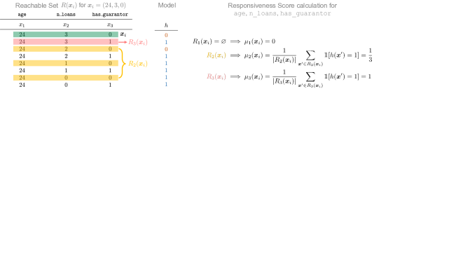
Figure 1: Feature-highlighting explanations for an individual denied credit by a logistic regression model for a lending task (see heloc, Section 4). We show explanations from top-scoring features using SHAP [40] (left) and responsiveness scores (right). As shown, SHAP highlights features immutable (Age, HistoryOfLatePayment, and HistoryOfDeliquency) or unresponsive (CreditLineUtilization). In contrast, explanations build using responsiveness score (right) only two features that provide recourse for the individual.

Related Work

Our work is related to a stream of research on post-hoc explanations  [47, 40, 48, 39, 64, 4, 41]. We focus on methods for feature attribution, which are designed to evaluate the importance of feature for a given prediction. Many methods are built for use cases in model development [e.g., 37, 34, 3], but are now used to construct “feature-highlighting explanations” to comply with regulations on explanations in consumer applications [see e.g., 6, 21].

Our work shows how feature attribution methods can inflict harm in such cases by highlighting reasons without recourse – i.e., by highlighting features, when acted upon, do not change the prediction – sometimes to consumers who are assigned fixed predictions. This is a failure mode that affects a broad class of local explainability techniques – adding to a growing literature on how local explanations are prone to manipulation [e.g., 38, 51, 52, 5, 26], and indeterminate [e.g., due to multiplicity 42, 59, 11, 8]. Our work complements impossibility results on recourse and feature attribution showing that attribution methods that satisfy completeness and linearity (e.g., SHAP) perform no better than random guessing when inferring model behavior (e.g., recourse)  [see e.g., 7, 22]. Here, we establish the prevalence of this effect empirically and develop a principled approach to mitigate it.

Our approach is related to a stream of work on algorithmic recourse [57, 31]. The vast majority of work on this topic develops algorithms for recourse provision – i.e., to present consumers with actions that can change the prediction a specific model [see e.g., 32]. Our goal is to highlight features that can be reliably changed to achieve recourse. To this end, responsiveness scores measure the number of actions on a single feature. Our approach builds on a line of work that elicits and enforces complex actionability constraints [57, 36]. Here, we use this machinery to represent actionability constraints at an instance level, and to generate a set of all points that a person can reach under a set of actionability constraints [36]. Our approach outputs feature responsiveness scores that can be used with any model, and can be adapted to address practical challenges in providing recourse – e.g., robustness [44, 45, 56] and causality [33, 13, 24].

2 Problem Statement

We formalize the problem of explaining the predictions of a machine learning model through feature attribution. We consider a standard classification task where we wish to predict a label $y\in\mathcal{Y}=\{0,1\}$ from a set of $d$ features $\bm{x}=[x_{1},x_{2},\ldots,x_{d}]\in\mathcal{X}\subseteq\mathbb{R}^{d}$. We assume that we given a model $h({}):\mathcal{X}\to\mathcal{Y}$ where each instance represents a person, and their features $\bm{x}_{i}\in\mathcal{X}$ encode semantically meaningful characteristics for the task at hand (e.g., age or income). We assume that the feature values are bounded so that $x_{j}\in[l_{j},u_{j}]$ and $\left\|\bm{x}\right\|\leq B$ for all $\bm{x}\in\mathcal{X}$ and $B$ sufficiently large.

We consider a task where we provide explanations to individuals who are adversely affected by the prediction of a given model (see e.g., [1, 55]). We assume that $h({\bm{x}_{i}})=1$ represents a target prediction that is desirable – e.g., $h({\bm{x}_{i}})=1$ if applicant $i$ is predicted to repay their loan within 2 years – and thus will explain the predictions for individuals where $h({\bm{x}_{i}})=0.$

Feature-Highlighting Explanations

Our goal is to construct explanations where each feature is responsive – i.e., can be changed independently to achieve recourse.

The standard practice of explaining predictions is to use feature-highlighting explanations [see e.g. 6]. These explanations consist of a list of “most important” features using a given method that we convert into a natural language description [e.g., a reason code 21].

Feature Attribution Methods

The standard approach to construct feature-highlighting explanation is to use feature attribution method [21].

Definition 1.

Given a model $h({}):\mathcal{X}\to\mathcal{Y}$ and its training dataset $\mathcal{D}{}=\{(\bm{x}_{i},y_{i})\}_{i=1}^{n}$, a feature attribution method for point $\bm{x}_{i}$ is a function $\bm{\phi}({\bm{x}_{i}\mid h({}),\mathcal{D}{}}):\mathcal{X}\to\mathbb{R}^{d}$, where the $j$th element of the output, $\phi_{j}({\bm{x}_{i}\mid h({}),\mathcal{D}{}})$ is the attribution for feature $j\in[d]$.

In what follows, we write $\bm{\phi}({\bm{x}_{i}})$ instead of $\bm{\phi}({\bm{x}_{i}\mid h({}),\mathcal{D}{}})$ when $h({})$ and $\mathcal{D}{}$ are clear from context. This function captures the behavior of several methods that are used to explain the prediction of a model in terms of its features:

• Local Linear Explainers [see e.g., 47, 65, 63, 16]: Given a model $h({})$ and a point $\bm{x}_{i}$, these methods fit a linear model $g:\mathbb{R}^{d}\to\mathbb{R}$ to approximate the decision boundary surrounding $\bm{x}_{i}$ such that $g(\bm{x}^{\prime})=\langle{\bm{\phi}(\bm{x}_{i})},{\bm{x}^{\prime}}\rangle$. The resulting attribution for each feature is its weight in $g$.

• Shapley Value Methods [see e.g., 40, 28, 23]: Given a model $h({})$ and a point $\bm{x}_{i}$, these methods cast features as players in a cooperative game, and estimate $\phi_{j}({\bm{x}_{i}})$ as the marginal contribution of feature $j$ to the prediction $h({\bm{x}_{i}})$ under basic axioms of social choice [50].

Given a model $h({})$ and its training dataset $\mathcal{D}$, the scores $\bm{\phi}(\bm{x}_{i})$ capture how each feature captures the prediction of a model at the $\bm{x}_{i}$ in different ways. In all cases, the scores satisfy the following properties:

• Relevance: A feature with an attribution score $\phi_{j}({\bm{x}_{i}})=0$ is not relevant to the prediction for $\bm{x}_{i}$ – i.e., it can be changed arbitrarily without changing the prediction [see e.g., the “missingness” axiom in 40].

• Strength: Features with larger attribution scores have larger impact on the prediction – i.e., if $|\phi_{j}({\bm{x}_{i}})|>|\phi_{j^{\prime}}({\bm{x}_{i}})|$, then feature $j$ has a stronger contribution to the prediction than feature $j^{\prime}$.

These properties allow model developers to comply with consumer protection rules, but can promote misinterpretation among consumers [34].

Reasons without Recourse

Features		Label Counts		Best Model
age $\geq$ 60	has_IRA	$n_{0}$	$n_{1}$	$h({\bm{x}})$
0	0	51	10	0
0	1	7	30	1
1	0	21	8	$0$
1	1	31	17	$0$

Table 1: Stylized lending task where the best model assigns fixed predictions. We predict $y\in\{0,1\}={\scriptsize{\small\texttt{repayment}}}$ from two binary features $(x_{1},x_{2})$ = ( age $\geq$ 60, has_IRA). We fit a classifier data with $n_{0}$ negative labels and $n_{1}$ positive labels for each $(x_{1},x_{2})\in\{0,1\}^{2}.$ Individuals with $x_{1}=1$ can only change their features to $(x_{1},x_{2})\in\{(1,0),(1,1)\}$ since age $\geq$ 60 is immutable and has_IRA is binary.

One failure mode of machine learning in consumer-facing applications is that models can assign fixed predictions – i.e., predictions that cannot be changed by their decision subjects (see e.g., Table 1). In lending, for example, fixed predictions inflict harm through preclusion – i.e., permanently barring consumers from access to credit. Fixed predictions are a recently-discovered failure mode [36], which must be mitigated through changes in feature construction, model development, or implementation (e.g.,using a separate model for re-applicants who are assigned fixed predictions). In practice, these instances are often left undetected. We can mitigate harm if instead of providing misleading explanations of fixed predictions they are flagged to model owners or auditors.

These issues stem from an oversight of actionability – how we can change the features of a model. On the one hand, models assign fixed predictions because they use features that can only be changed in specific ways. On the other, we are unable to detect these instances through feature attribution methods because they are designed to explain a prediction, rather than how it can be changed.

Accounting for Actionability

Given these challenges, we introduce machinery to capture how features can be changed at the instance level. For example, a change in one feature might necessitate a change in another; this makes strictly independent changes to certain features infeasible.

Definition 2.

An action is a vector $\bm{a}=[a_{1},\ldots,a_{d}]\in\mathbb{R}^{d}$ that a person can perform to change their features from $\bm{x}_{i}$ to $\bm{x}_{i}+\bm{a}=\bm{x}^{\prime}\in\mathcal{X}$. Given a point $\bm{x}_{i}\in\mathcal{X}$, the action set $A({\bm{x}_{i}})$ contains all possible actions for $\bm{x}_{i}$. We assume that every action set contains the null action $\bm{\emptyset}\in A({\bm{x}_{i}})$.

Action sets captures how we can change features from a given point as a set of actionability constraints. As shown in Table 2, we can elicit complex constraints from human experts in natural language, and convert them into equations that we can embed into an optimization problem. In this way, we can enforce actionability in – for example – algorithms to find recourse actions [see e.g., 57, 36].

Class		Example	Features	Actionability Constraint
Immutability		age cannot change	$x_{j}={\small\texttt{age}}$	$a_{j}=0$
Monotonicity		recent_payment can only increase	$x_{j}={\small\texttt{recent\_payment}}$	$a_{j}\geq 0$
Integrality		late_payments must be positive integer $\leq 12$	$x_{j}={\small\texttt{late\_payments}}$	$a_{j}\in\mathbb{Z}^{+}\cap[0-x_{j},12-x_{j}]$
Encoding Validity		preserve one-hot encoding of categorical feature housing_status $\in\{{\small\texttt{own}},{\small\texttt{rent}},{\small\texttt{other}}\}$	$x_{k}={\small\texttt{housing\_status=own}}$ $x_{l}={\small\texttt{housing\_status=rent}}$ $x_{m}={\small\texttt{housing\_status=other}}$	$a_{j}+x_{j}\in\{0,1\}~{}\textrm{for}~{}j\in\{k,l,m\}$ $\sum_{j\in\{k,l,m\}}a_{j}+x_{j}=1$
Logical Implication		if ${\small\texttt{has\_savings\_account}}={\small\texttt{TRUE}}$ then ${\small\texttt{savings\_account\_balance}}\geq 0$ else ${\small\texttt{savings\_account\_balance}}=0$	$x_{j}={\small\texttt{has\_savings\_account}}$ $x_{k}={\small\texttt{savings\_account\_balance}}$	$a_{j}+x_{j}\in\{0,1\}$ $a_{k}+x_{k}\in[0,10^{12}]$ $a_{j}+x_{j}\leq 10^{12}(x_{k}+a_{k})$
Causal Implication		if years_of_account_history increases then age will increase commensurately	$x_{j}={\small\texttt{years\_of\_account\_history}}$ $x_{k}={\small\texttt{age}}$	$x_{j}+a_{j}\leq x_{k}+\delta_{k}$ $\delta_{k}\in[0,100]$

Table 2: Examples of actionability constraints on semantically meaningful features for a lending task (see Section A for additional examples). Each constraint can be expressed in natural language and embedded into an optimization problem using standard techniques in mathematical programming [see, e.g., 61].

To highlight features that are responsive, we must assign a score to features that accounts for actionability constraints. In practice, the actionability constraints for a given feature will include constraints that pertain to the feature as well as other features. We refer to the features that may change as a result of interventions on feature $j$ as downstream features, $C_{j}$.

Definition 3.

Given an action set $A({\bm{x}_{i}})$ for a point $\bm{x}_{i}\in\mathcal{X}$, the action set for feature $j\in[d]$ is:

$$A_{j}({\bm{x}_{i}}):=\{\bm{a}\in A({\bm{x}_{i}})~{}|~{}\bm{a}_{j}\neq 0\wedge\bm{a}_{k}=0,k\in[d]\setminus C_{j}\}$$

Here, the downstream set $C_{j}:=\{k\in[d]\setminus\{j\}~{}|~{}\bm{a}_{j}\neq 0\implies\bm{a}_{k}\neq 0~{}~{}\forall\bm{a}\in A({\bm{x}})\}$ is the subset of all features that must change as a result of interventions on feature $j$. Definition 3 captures cases where actions on a feature can induce changes in other features. Such cases can stem from deterministic causal relationships – e.g., increasing years_of_account_history should lead to a commensurate change in age. In general, they can capture dependencies that would not be included in a traditional causal graph – e.g., changing a categorical attribute will require switching a binary feature “off” while turning another binary feature “on” (so that $x_{j}=1\to 0\implies x_{j}^{\prime}=0\to 1$).

3 Measuring Feature Responsiveness

In this section, we introduce our main technical contribution – the responsiveness score. We first define the responsiveness score, then discuss its interpretation and computation.

3.1 Responsiveness Scores

Our goal is to measure the responsiveness of the prediction of a model at a point $\bm{x}_{i}$ with respect to the set of feasible actions on specific features. We propose to measure the sensitivity for each feature through the feature responsiveness score.

Definition 4.

Given a model $h({}):\mathcal{X}\to\mathcal{Y}$, a point $\bm{x}_{i}$ with action set $A({\bm{x}_{i}})$ and feature $j\in[d]$, the responsiveness score for feature $j$ is defined as:

$$\mu_{j}({\bm{x}_{i}\mid h({}),A({\bm{x}_{i}})}):=\textnormal{Pr}(h({\bm{x}^{\prime}})=1\mid\bm{x}^{\prime}=\bm{x}_{i}+\bm{a},\bm{a}\in A_{j}({\bm{x}_{i}})$$

The responsive score for a feature $j$ captures the proportion of single-feature actions on feature $j$ that change the prediction of a model $h({})$ at $\bm{x}_{i}$. In what follows, we write $\mu_{j}({\bm{x}})$ instead of $\mu_{j}({\bm{x}\mid h({}),A({\bm{x}_{i}})})$ when $h({})$ and $A({\bm{x}_{i}})$ are clear from context. Given a feature where $\mu_{j}({\bm{x}_{i}})=p$, we know that $100(p)\%$ of the single-feature actions on $j$, $\bm{a}\in A_{j}({\bm{x}_{i}})$ will change the prediction of the model. Thus, all actions to a feature where $\mu_{j}({\bm{x}_{i}})=0$ would not change the prediction while all actions on a feature where $\mu_{j}({\bm{x}_{i}})=1$ would result in a different prediction.

These interpretations are contingent on the actionability constraints used to compute the responsiveness score. In the simplest case, actionability constraints encode indisputable constraints on how a feature can be changed (e.g., feature encoding or physical limits) and so the responsiveness score for a given feature represent an upper bound on responsiveness: “at most $100\mu_{j}({\bm{x}_{i}})$% of single-feature actions on feature $j$ attain a desired prediction.” Such constraints let us flag undeniable instances of harm. More generally, actionability constraints encode information about how other features are expected to vary when a single feature is changed. For example, if a model has a feature indicating the job rank of an individual, we can create actionability constraints that encode the expectation that if job rank increases, so does income.

Safeguards for Consumer Protection

One benefit of responsiveness scores is that we can reliably use them to detect when consumers are assigned fixed predictions, and when feature-based explanations can provide recourse.

Remark 1.

Given a model $h({}):\mathcal{X}\to\mathcal{Y}$, let $\mu_{1}({\bm{x}_{i}}),\ldots,\mu_{d}({\bm{x}_{i}})$ denote the responsiveness scores of $\bm{x}_{i}\in\mathcal{X}$ with respect to the action set $A({\bm{x}_{i}}).$

1. If $\mu_{j}({\bm{x}_{i}})>0$ for some feature $j\in[d]$, then $h({})$ can provide recourse to $\bm{x}_{i}$ through a single-feature action on $j$.

2. If $\mu_{j}({\bm{x}_{i}})=0$ for all features $j\in[d]$, then either: (i) $h({})$assigns a fixed prediction to $\bm{x}_{i}$, or (ii) $h({})$can only provide recourse to $\bm{x}_{i}$ through actions that alter two or more features.

Remark 1a) states that every person ($\bm{x}_{i}$) who receives a positive responsiveness score for at least one feature has recourse. This implies that when we construct feature-highlighting explanations using the top-$k$ responsiveness scores, we will only provide explanations to individuals who have recourse. Remark 1b) also illustrates how the responsiveness scores can flag for potential harm when $\mu_{j}({\bm{x}_{i}})=0$ and allows us to mitigate harm on a case by case basis. In case b)(i) – where a person is assigned fixed predictions – we would refrain from providing explanations to avoid misleading consumers, and flag the issue so that model development can be potentially revisited. In case b)(ii) – where a person is assigned predictions that can change through multiple actions – we could provide explanations that highlight subsets of responsive features, include explicit warning against presumptions of feature independence, or proceed in a similar manner to case b)(i).

3.2 Computing Scores with Reachable Sets

Figure 2: Simple example of how to compute responsiveness scores involving three independent features. age is an immutable feature, n_loans is a discrete feature taking values from 0 to 3 and has_guarantor is a binary feature. The original prediction of 0 is shown in the row highlighted in green. Single-feature actions for n_loans, has_guarantor are highlighted yellow and red respectively. We can see that we can construct a complete reachable set and directly calculate the responsiveness score for discrete datasets. The responsiveness score for age is 0 since it is immutable.

We compute responsiveness scores using a reachable set:

Definition 5.

Given a point $\bm{x}_{i}$ and its action set $A({\bm{x}_{i}})$, we refer to the set of all points that are attainable through actions in $A({\bm{x}})$ as the reachable set: $R({\bm{x}_{i}}):=\{\bm{x}_{i}+\bm{a}\mid\bm{a}\in A({\bm{x}_{i}})\}$. We refer to the subset of points that are reachable through actions on feature $j\in[d]$ as the reachable set for feature $j$ and denote it as: $R_{j}({\bm{x}_{i}}):=\{\bm{x}_{i}+\bm{a}^{\prime}\mid\bm{a}^{\prime}\in A_{j}({\bm{x}_{i}})\}$.

Reachable sets represents an alternative way to store and process information about actionability at the instance level. In particular, a reachable set $R({\bm{x}_{i}})$ encodes this information as a set of feature vectors that can be reached through feasible actions. Given reachable sets for each feature $R_{j}({\bm{x}_{i}})$ for $j\in[d]$, we can calculate responsiveness scores (see Definition 4) for a model by querying its predictions (see Fig. 2). This has the benefits that: (1) it can work with any model; (2) we only need to compute the reachable set once; and (3) it can allow us to evaluate other notions of responsiveness.

Enumeration for Discrete Features

When dealing with discrete feature spaces, we can obtain a complete reachable set through enumeration following an approach of Kothari et al. [36]. Given a point $\bm{x}_{i}$ and its action set $A({\bm{x}_{i}})$, this approach returns a set of all reachable points. Given a complete reachable set, we can calculate the responsiveness score of feature $j$ by evaluating the model $h({})$ on points reachable via single-feature actions on $j$ (see Fig. 2). This approach can certify when an individual cannot change the prediction of a model. Unfortunately, the reachable set grows exponentially with the number of actionable features, which can lead to practical challenges in storage and compute.

Sampling for Continuous Features

The enumeration technique described above is infeasible when we wish to evaluate the responsiveness of a continuous feature, or when a feature has downstream effects on continuous features. In such cases, we estimate the responsiveness score for feature $j$ by drawing a uniform sample of reachable points from $R_{j}({\bm{x}_{i}}).$ Given a feature without downstream effects – i.e., without downstream features so that $|C_{j}|=0$ – we can sample values from $[l_{j},u_{j}]$. When features have downstream effects, we can apply a rejection sampling procedure where we first sample values for all features from $[l_{j},u_{j}]$ and reject values that violate actionability constraints.

Definition 6.

Given a point $\bm{x}_{i}\in\mathcal{X}$, let $\hat{R}_{j}({\bm{x}_{i}})$ denote a sample of $N{}$ points drawn uniformly from the reachable set for feature $j$, $R_{j}({\bm{x}_{i}})$. Given any model $h({}):\mathcal{X}\to\mathcal{Y}$, we can estimate the responsiveness score for feature $j$ as

$$\hat{\mu}_{j}({\bm{x}_{i}}):=\frac{1}{N}\sum_{\bm{x}^{\prime}\in\hat{R}_{j}({\bm{x}_{i}})}\mathbbm{1}[h({\bm{x}^{\prime}})=1$$

When the samples are drawn uniformly from $R_{j}({\bm{x}_{i}})$, the number of responsive predictions $S\sim\textrm{Bin}(N,\mu_{j}({\bm{x}_{i}}))$. We can then quantify the uncertainty associated with our estimate $\hat{\mu}_{j}({\bm{x}_{i}})$:

Proposition 2.

Given a level of significance $\alpha\in(0,1)$, the $100(1-\alpha)\%$ confidence interval for $\mu_{j}({\bm{x}_{i}})$ is:

$$\tilde{\mu}_{j}({\bm{x}_{i}})\;\pm\;\kappa\sqrt{\frac{1}{\tilde{N}}\tilde{\mu}_{j}({\bm{x}_{i}})(1-\tilde{\mu}_{j}({\bm{x}_{i}}))}$$

Here: $\kappa:=\Phi^{-1}(1-\tfrac{\alpha}{2})$, $\Phi(\cdot)$ is the Normal CDF, and $\tilde{\mu}_{j}({\bm{x}_{i}}):=\frac{1}{N+\kappa^{2}}\left(S+\frac{\kappa^{2}}{2}\right)$ is the corrected estimator.

We can alter two parameters to adjust the uncertainty: the level of significance $\alpha$ and the sample size $N$. For a fixed $N$, a larger $\alpha$ will yield a narrower confidence interval at a lower confidence level. Similarly, with a fixed $\alpha$, we can adjust $N$ to attain a desired level of certainty for the estimate $\hat{\mu}_{j}({\bm{x}_{i}})$. For example, given $\alpha=0.05$, $N>42$ would ensure that the width of the confidence interval surrounding $\hat{\mu}_{j}({\bm{x}_{i}})$ is at most 0.1 when we don’t observe any points with the target prediction – i.e. $S=0$. Note that we use a correction upon the standard binomial confidence interval formulation to improve coverage when $\mu_{j}({\bm{x}_{i}})=0$ or $1$ [see 10].

This is a general-purpose approach that can compute responsiveness scores for features that are continuous or discrete. In settings where we are computing the responsiveness score of a discrete feature, we can reap the benefits of responsiveness using a small sample of reachable points. This approach avoids the computation and storage costs of enumeration but sacrifices the ability to identify individuals with fixed predictions with complete certainty.

Discussion

One of the benefits of working with reachable sets is that they can readily be extended to handle other desiderata by weighing and filtering reachable points. As an example, we can highlight features that are robust to changes through a robust variant defined below.

Definition 7.

Given a model $h({}):\mathcal{X}\to\mathcal{Y}$, a point $\bm{x}_{i}$ with action set $A({\bm{x}_{i}})$ and feature $j\in[d]$, the robust responsiveness score for feature $j$ measures the probability that an action on feature $j$ will flip the prediction regardless of the actions on other features:

$$\nu_{j}({\bm{x}_{i}\mid h({}),A({\bm{x}_{i}})}):=\textnormal{Pr}(h({\bm{x}^{\prime}})=1\mid\bm{x}^{\prime}=\bm{x}_{i}+\bm{a},\bm{a}_{j}\neq 0,\bm{a}\in A({x})$$

This variant can measure the prevalence of actions that would change a prediction even as other features change [see e.g., 44]. We can calculate the robust responsiveness score by enumerating a subset of the entire reachable set $R({\bm{x}_{i}})$ containing points reachable by all actions that alter feature $j$.

4 Experiments

We present an empirical study on the responsiveness of explanations. Our goals are: (1) to evaluate how our approach can support recourse and flag fixed predictions; and (2) to demonstrate the limitations of existing feature attribution methods in practice. We include additional results and details in Sections A and B, and code to reproduce these results at the project repository.

Setup

We work with three classification datasets from consumer finance that are publicly available and used in prior work (see Section A for details). Here, each instance represents a consumer and each label indicates whether they will repay a loan. For each dataset, we define inherent actionability constraints that capture indisputable requirements and that apply to all individuals – e.g., no changes for immutable and protected attributes, changes must preserve feature encoding and adhere to deterministic causal effects (see Section A).

We split each dataset into a training sample (80%; to train models and tune hyperparameters) and a test sample (20%; to evaluate out-of-sample performance). We train classifiers using (1) logistic regression ($\mathsf{LR}$), (2) XGBoost ($\mathsf{XGB}$), and (3) random forests ($\mathsf{RF}$). For each model, we construct a feature-based explanation for each individual who is denied credit by listing the top-$k$ highest-scoring features from the following methods:

• Feature Responsiveness Score (RESP): We compute the score in Definition 4 using the procedure in Section 3.2, and the actionability constraints in Section A.

• Standard Feature Attribution: We consider local feature attribution methods that are model-agnostic and widely used in the lending industry [21]: Shapley additive explanation (SHAP)  [40]; and local interpretable model-agnostic explanations (LIME)  [47].

• Actionable Feature Attribution: We also consider action-aware variants of feature attribution methods SHAP-AW and LIME-AW, which seek to promote responsiveness by setting the scores for immutable features to 0 such that $\phi_{j}({\bm{x}_{i}})\leftarrow 0$ when feature $j$ is immutable.

Dataset	Metrics	$\mathsf{LR}$	$\mathsf{RF}$	$\mathsf{XGB}$
heloc $n={5,842}$ $d={43}$ ($d_{A}={31}$) FICO [20]	% Denied $\Rsh$  % Fixed $\Rsh$  % 1-D Rec $\Rsh$  % n-D Rec	56.1% 19.1% 44.4% 36.6%	58.3% 28.1% 34.6% 37.4%	57.0% 49.1% 29.8% 21.2%
german $n={1,000}$ $d={36}$ ($d_{A}={9}$) Dua and Graff [14]	% Denied $\Rsh$  % Fixed $\Rsh$  % 1-D Rec $\Rsh$  % n-D Rec	22.9% 7.4% 73.4% 19.2%	17.5% 29.1% 51.4% 19.4%	22.0% 15.5% 65.5% 19.1%
givemecredit $n={120,268}$ $d={23}$ ($d_{A}={13}$) Kaggle [29]	% Denied $\Rsh$  % Fixed $\Rsh$  % 1-D Rec $\Rsh$  % n-D Rec	24.6% 15.6% 72.4% 12.0%	24.7% 0.2% 93.2% 6.6%	24.8% 11.5% 76.0% 12.5%

Table 3: Recourse feasibility across datasets and model classes. % Denied – the fraction of individuals denied credit by a model; % 1-D – the fraction of denied individuals who can achieve recourse with actions that alter a single feature; % n-D – the fraction of denied individuals who can achieve recourse with actions that alter 2 or more features; and % Fixed – the fraction of denied individuals who are assigned a fixed prediction (in red if $>0$).

Results

We summarize the viability of promoting recourse using feature-highlighting explanations in Table 3, and the responsiveness of explanations from each method in Table 4. We evaluate explanations built using the top-4 scoring features from each method, which reflects the recommended number of reasons to include in an adverse action notice required by the U.S. Equal Credit Opportunity Act [see 2, 6].

Our results in Table 3 show that models admit features that allow some individuals to change them to attain a desired prediction (29.8% to 93.2% across models and datasets). At the same time, they reveal their potential to mislead individuals who are assigned fixed predictions (i.e., 0.2% to 49.1% across all models and datasets). For example, given the $\mathsf{LR}$ model for the heloc dataset, we would present an explanation to 56.1% of individuals who are a denied loan. Among them, 44.4% can achieve recourse through single-feature actions; 35.6% can only achieve recourse through joint actions; and 19.1% have no path to recourse because they receive a fixed prediction.

On Responsiveness Scores

Our results in Table 4 show how our approach can support consumers by presenting responsive features and by flagging instances where explanations may be misleading. Explanations are only provided to individuals who can achieve recourse through a single-feature action, and are given to all such individuals (the values for % Presented with Reasons in Table 4 match the values for % 1-D Rec in Table 3). When we construct feature-based explanations using responsiveness scores, we present individuals with explanations that only contain responsive features, achieving 100% on the % All Reasons Responsive metric across datasets and models. This may result in explanations that highlight fewer reasons on average—for example, individuals receiving explanations from the $\mathsf{LR}$ model on german receive 1.9 out of 4 reasons on average. This behavior can mitigate harm as we avoid presenting explanations to individuals with fixed predictions or those who require joint actions to change their outcomes.

On Feature Attribution Scores

Our results show how standard methods for feature attribution can output explanations that are ineffective and potentially misleading. For example, under the $\mathsf{LR}$ model for the heloc dataset, we find that 82% and 75.6% of explanations from LIME and SHAP include 4/4 unresponsive features respectively. This behavior arises as a result of algorithm design, as the scores do not account for responsiveness nor actionability. This results in two key problems:

• Low Scores for Responsive Features: Methods can assign low scores to responsive features. On the heloc dataset, for example, 44.4% of denied individuals by the $\mathsf{LR}$ model can achieve recourse by altering a single feature. However, explanations built using LIME and SHAP fail to include them since their scoring mechanisms do not account for feature responsiveness. For instance, an individual could achieve recourse by acting on NumRevolvingTrades, but a feature-based explanation produced by LIME does not include it, as it assigns higher scores to four other features that are unresponsive. We also observe this phenomenon beyond the top-4 features in Fig. 3.

• Reasons without Recourse: Methods provide explanations to individuals with fixed predictions. On the heloc dataset, the $\mathsf{LR}$ model assigns a fixed prediction to 19.1% of denied individuals. In such cases, LIME and SHAP, and their variants offer explanations, even though it is impossible for them to achieve recourse. These explanations may mislead individuals by highlighting features that are salient to the prediction and could be changed, but would not lead to recourse. For example, an explanation from SHAP for an individual with a fixed prediction includes AvgYearsInFile and NetFractionRevolvingBurden – both of which are mutable but not actionable.

		$\mathsf{LR}$					$\mathsf{XGB}$
		All Features		Actionable Features			All Features		Actionable Features
Dataset	Metrics	LIME	SHAP	LIME-AW	SHAP-AW	RESP	LIME	SHAP	LIME-AW	SHAP-AW	RESP
heloc $n={5,842}$ $d={43}$ ($d_{A}={31}$) FICO [20]	% Presented with Explanations $\Rsh$  % All Unresponsive $\Rsh$  % At Least 1 Responsive $\Rsh$  % All Responsive $\Rsh$  Mean # of Features	100.0% 82.0% 18.0% 0.0% 4.0	100.0% 75.6% 24.4% 0.0% 4.0	100.0% 64.7% 35.3% 0.2% 4.0	100.0% 64.7% 35.3% 0.2% 4.0	44.4% 0.0% 100.0% 100.0% 2.4	100.0% 92.6% 7.4% 0.0% 4.0	100.0% 80.7% 19.3% 0.0% 4.0	100.0% 77.5% 22.5% 0.0% 4.0	100.0% 75.1% 24.9% 0.0% 4.0	29.8% 0.0% 100.0% 100.0% 2.7
german $n={1,000}$ $d={36}$ ($d_{A}={9}$) Dua and Graff [14]	% Presented with Explanations $\Rsh$  % All Unresponsive $\Rsh$  % At Least 1 Responsive $\Rsh$  % All Responsive $\Rsh$  Mean # of Features	100.0% 100.0% 0.0% 0.0% 4.0	100.0% 100.0% 0.0% 0.0% 4.0	100.0% 62.9% 37.1% 0.0% 4.0	100.0% 66.4% 33.6% 0.0% 4.0	73.4% 0.0% 100.0% 100.0% 1.9	100.0% 100.0% 0.0% 0.0% 4.0	100.0% 83.2% 16.8% 0.0% 4.0	100.0% 64.5% 35.5% 0.0% 4.0	100.0% 66.8% 33.2% 0.0% 4.0	65.5% 0.0% 100.0% 100.0% 2.0
givemecredit $n={120,268}$ $d={23}$ ($d_{A}={13}$) Kaggle [29]	% Presented with Explanations $\Rsh$  % All Unresponsive $\Rsh$  % At Least 1 Responsive $\Rsh$  % All Responsive $\Rsh$  Mean # of Features	100.0% 55.8% 44.2% 0.0% 4.0	100.0% 45.5% 54.5% 0.0% 4.0	100.0% 50.7% 49.3% 5.5% 4.0	100.0% 31.8% 68.2% 23.1% 4.0	72.4% 0.0% 100.0% 100.0% 2.4	100.0% 40.9% 59.1% 0.0% 4.0	100.0% 51.3% 48.7% 0.0% 4.0	100.0% 30.9% 69.1% 5.4% 4.0	100.0% 40.6% 59.4% 3.7% 4.0	76.0% 0.0% 100.0% 100.0% 2.6

Table 4: Responsiveness of feature-based explanations for $\mathsf{LR}$ and $\mathsf{XGB}$ models across all methods and datasets (We defer results for $\mathsf{RF}$ to Section B.2 for clarity). For each model, we generate feature-based explanations for individuals denied a loan, highlighting up to 4 top-scoring features from a given feature attribution method. For each method, we report the proportion of individuals receiving an explanation (% Presented with Explanations); the mean number of features per explanation (Mean # of Features); and the proportion of explanations that highlight only unresponsive features (% All Unresponsive), include at least one responsive feature (At Least 1 Responsive), or highlight only responsive features (All Responsive, in bold). Methods that return only unresponsive explanations are marked in red.

On Adapting Existing Methods

Seeing how responsiveness is inherently tied to actionability, we study the potential to improve responsiveness through action-aware variants of SHAP and LIME – SHAP-AW and LIME-AW. We consider a simple post-processing strategy where we only construct explanations using features that are mutable. This reflects a common belief surrounding actionability is that we can find ways to account for it by post-processing [e.g., 43, 30]. Our results show this approach can improve the responsiveness of explanations – as we observe marginal improvements when switching from SHAP and LIME to SHAP-AW and LIME-AW for all models and datasets in Table 4. For example, when we provide explanations for $\mathsf{LR}$ model on heloc, switching from SHAP to SHAP-AW improves the proportion of explanations that contain at least one responsive feature from $24.4\%$ to $35.3\%.$ As a result, more consumers could achieve recourse based on explanations with at least one responsive feature. We observe SHAP-AW’s increased tendency to return responsive features at higher ranks in Fig. 3 as well: the distribution of the % of times the feature was responsive at each rank shifts slightly upward when we adapt SHAP to SHAP-AW. Nevertheless, SHAP-AW and LIME-AW explanations still contain unresponsive reasons. In the heloc dataset, SHAP-AW and LIME-AW returned explanations where every reason is responsive 0.2% of the time under the $\mathsf{LR}$ model. In other words, 98% of the explanations given to denied consumers contained at least one unresponsive feature. This occurs because LIME-AW and SHAP-AW still suffer from the same drawbacks as their original counterparts, albeit to a lesser extent. They attribute scores to features that are not responsive when there are other responsive features or have exhausted the list of such features. Overall, these results show that they still fall short in providing responsive explanations.

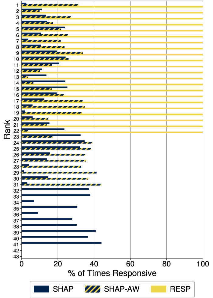
Figure 3: Responsiveness of top-scoring features for individuals who are denied credit by the $\mathsf{LR}$ model on the heloc dataset for using SHAP, SHAP-AW and RESP. For each method, we report the proportion of instances where a feature assigned the $k$-th largest score is responsive – i.e. has at least one single-feature action that leads to recourse. Higher-ranking SHAP features are rarely responsive. SHAP-AW performs better by assigning responsive features to the top more often, but only marginally. RESPonly assigns ranks when features are responsive. We only compute scores for individuals who are denied (i.e., 24%), and only show bars for features that receive a non-zero attribution score. We provide analogous plots for other datasets, model classes and methods in Section C.

5 Concluding Remarks

Explanations are often seen as a strategy to protect individuals from harm when machine learning models are applied in domains like lending and hiring. Our work reveals how this strategy can backfire by highlighting unresponsive features and overlooking fixed predictions. We find that common feature attribution methods exhibit both of these failure modes, leading to situations where consumers are given reasons without recourse. Our work addresses these limitations by developing a feature attribution method that measures responsiveness—i.e., the probability that a feature can be changed in a way that leads to recourse. These scores can readily replace the scores currently used to comply with regulations. In doing so, we can strengthen consumer protection by highlighting features that enable recourse when possible and flagging instances where recourse is unattainable. Our results demonstrate the benefits of developing standalone methods to address specific goals—whether for recourse, rectification, or anti-discrimination. By adopting specialized approaches, we can achieve more effective consumer protection.

Limitations

The main limitations of our work stem from assumptions about actionability and responsiveness. Our approach relies on the validity of actionability assumptions within an action set. When defining this set to encode indisputable constraints, as in Section 4, responsiveness scores can flag individuals with fixed predictions. However, presented features may not achieve recourse due to individual constraints. To mitigate this, we can highlight features achieving a threshold responsiveness or elicit constraints from decision subjects [see e.g., 17, 12, 35]. A broader limitation is that our machinery only represents a subset of constraints considered in causal algorithmic recourse literature. It can represent cases with deterministic causal effects but excludes scenarios where interventions induce probabilistic effects on downstream features [33, 13, 58]. In principle, our approach can incorporate such assumptions: given an individual probabilistic graphical model, we can compute a responsiveness score reflecting the expected recourse rate. The key challenge lies in validating causal assumptions at an individual level. This reflects a practical bottleneck that requires further study and may require an approach to measure responsiveness in a way that is robustness to misspecifcation.

Acknowledgements

This work is supported by the National Science Foundation (NSF) under grant IIS-2313105.

A Datasets and Actionability Constraints

A.1 heloc

A.1.1 Dataset Description

The FICO dataset was created to predict repayment on Home Equity Line of Credit (HELOC) applications. HELOC credit lines are loans that use people’s homes as collateral. The dataset is used by lenders to determine how much credit should be granted. The anonymized version of the HELOC dataset was created by FICO to present an explainable machine learning challenge for a prize.

Each instance in the dataset is a real credit application for HELOC credit; it’s an application that a single person submitted and contains information about that person. There are $n=10,459$ instances, each consisting of $d=23$ features. These features are either binary or discrete. The label, RiskPerformance, is a binary assessment of the risk of repayment based on the 23 predictors. A value of 1 means the person hasn’t been more than 90 days overdue on their payments in the last 2 years; a value of 0 means they have at least once. There are some repeated instances; there are 9,871 unique rows. The dataset is self-contained and has been anonymized for public use in the explainability challenge. It doesn’t use any protected attributes like race and gender.

A.1.2 Actionability Constraints

Name	Type	LB	UB	mutability
ExternalRiskEstimate_geq_40	$\{0,1\}$	0	1	no
ExternalRiskEstimate_geq_50	$\{0,1\}$	0	1	no
ExternalRiskEstimate_geq_60	$\{0,1\}$	0	1	no
ExternalRiskEstimate_geq_70	$\{0,1\}$	0	1	no
ExternalRiskEstimate_geq_80	$\{0,1\}$	0	1	no
YearsOfAccountHistory	$\mathbb{Z}$	0	50	no
AvgYearsInFile_geq_3	$\{0,1\}$	0	1	only increases
AvgYearsInFile_geq_5	$\{0,1\}$	0	1	only increases
AvgYearsInFile_geq_7	$\{0,1\}$	0	1	only increases
MostRecentTradeWithinLastYear	$\{0,1\}$	0	1	yes
MostRecentTradeWithinLast2Years	$\{0,1\}$	0	1	yes
AnyDerogatoryComment	$\{0,1\}$	0	1	no
AnyTrade120DaysDelq	$\{0,1\}$	0	1	no
AnyTrade90DaysDelq	$\{0,1\}$	0	1	no
AnyTrade60DaysDelq	$\{0,1\}$	0	1	no
AnyTrade30DaysDelq	$\{0,1\}$	0	1	no
NoDelqEver	$\{0,1\}$	0	1	no
YearsSinceLastDelqTrade_leq_1	$\{0,1\}$	0	1	only increases
YearsSinceLastDelqTrade_leq_3	$\{0,1\}$	0	1	only increases
YearsSinceLastDelqTrade_leq_5	$\{0,1\}$	0	1	only increases
NumInstallTrades_geq_2	$\{0,1\}$	0	1	only increases
NumInstallTradesWBalance_geq_2	$\{0,1\}$	0	1	only increases
NumRevolvingTrades_geq_2	$\{0,1\}$	0	1	only increases
NumRevolvingTradesWBalance_geq_2	$\{0,1\}$	0	1	only increases
NumInstallTrades_geq_3	$\{0,1\}$	0	1	only increases
NumInstallTradesWBalance_geq_3	$\{0,1\}$	0	1	only increases
NumRevolvingTrades_geq_3	$\{0,1\}$	0	1	only increases
NumRevolvingTradesWBalance_geq_3	$\{0,1\}$	0	1	only increases
NumInstallTrades_geq_5	$\{0,1\}$	0	1	only increases
NumInstallTradesWBalance_geq_5	$\{0,1\}$	0	1	only increases
NumRevolvingTrades_geq_5	$\{0,1\}$	0	1	only increases
NumRevolvingTradesWBalance_geq_5	$\{0,1\}$	0	1	only increases
NumInstallTrades_geq_7	$\{0,1\}$	0	1	only increases
NumInstallTradesWBalance_geq_7	$\{0,1\}$	0	1	only increases
NumRevolvingTrades_geq_7	$\{0,1\}$	0	1	only increases
NumRevolvingTradesWBalance_geq_7	$\{0,1\}$	0	1	only increases
NetFractionInstallBurden_geq_10	$\{0,1\}$	0	1	only increases
NetFractionInstallBurden_geq_20	$\{0,1\}$	0	1	only increases
NetFractionInstallBurden_geq_50	$\{0,1\}$	0	1	only increases
NetFractionRevolvingBurden_geq_10	$\{0,1\}$	0	1	only increases
NetFractionRevolvingBurden_geq_20	$\{0,1\}$	0	1	only increases
NetFractionRevolvingBurden_geq_50	$\{0,1\}$	0	1	only increases
NumBank2NatlTradesWHighUtilizationGeq2	$\{0,1\}$	0	1	only increases

Table 5: Table of Separable Actionability Constraints for the heloc dataset. Includes bounds and monotonicity constraints.

Joint Actionability Constraints:

1. DirectionalLinkage: Actions on NumRevolvingTradesWBalance$\geq$2 will induce to actions on [’NumRevolvingTrades$\geq$2’]. Each unit change in NumRevolvingTradesWBalance$\geq$2 leads to:1.00-unit change in NumRevolvingTrades$\geq$2

2. DirectionalLinkage: Actions on NumInstallTradesWBalance$\geq$2 will induce to actions on [’NumInstallTrades$\geq$2’]. Each unit change in NumInstallTradesWBalance$\geq$2 leads to:1.00-unit change in NumInstallTrades$\geq$2

3. DirectionalLinkage: Actions on NumRevolvingTradesWBalance$\geq$3 will induce to actions on [’NumRevolvingTrades$\geq$3’]. Each unit change in NumRevolvingTradesWBalance$\geq$3 leads to:1.00-unit change in NumRevolvingTrades$\geq$3

4. DirectionalLinkage: Actions on NumInstallTradesWBalance$\geq$3 will induce to actions on [’NumInstallTrades$\geq$3’]. Each unit change in NumInstallTradesWBalance$\geq$3 leads to:1.00-unit change in NumInstallTrades$\geq$3

5. DirectionalLinkage: Actions on NumRevolvingTradesWBalance$\geq$5 will induce to actions on [’NumRevolvingTrades$\geq$5’]. Each unit change in NumRevolvingTradesWBalance$\geq$5 leads to:1.00-unit change in NumRevolvingTrades$\geq$5

6. DirectionalLinkage: Actions on NumInstallTradesWBalance$\geq$5 will induce to actions on [’NumInstallTrades$\geq$5’]. Each unit change in NumInstallTradesWBalance$\geq$5 leads to:1.00-unit change in NumInstallTrades$\geq$5

7. DirectionalLinkage: Actions on NumRevolvingTradesWBalance$\geq$7 will induce to actions on [’NumRevolvingTrades$\geq$7’]. Each unit change in NumRevolvingTradesWBalance$\geq$7 leads to:1.00-unit change in NumRevolvingTrades$\geq$7

8. DirectionalLinkage: Actions on NumInstallTradesWBalance$\geq$7 will induce to actions on [’NumInstallTrades$\geq$7’]. Each unit change in NumInstallTradesWBalance$\geq$7 leads to:1.00-unit change in NumInstallTrades$\geq$7

9. DirectionalLinkage: Actions on YearsSinceLastDelqTrade$\leq$1 will induce to actions on [’YearsOfAccountHistory’]. Each unit change in YearsSinceLastDelqTrade$\leq$1 leads to:-1.00-unit change in YearsOfAccountHistory

10. DirectionalLinkage: Actions on YearsSinceLastDelqTrade$\leq$3 will induce to actions on [’YearsOfAccountHistory’]. Each unit change in YearsSinceLastDelqTrade$\leq$3 leads to:-3.00-unit change in YearsOfAccountHistory

11. DirectionalLinkage: Actions on YearsSinceLastDelqTrade$\leq$5 will induce to actions on [’YearsOfAccountHistory’]. Each unit change in YearsSinceLastDelqTrade$\leq$5 leads to:-5.00-unit change in YearsOfAccountHistory

12. ReachabilityConstraint: The values of [MostRecentTradeWithinLastYear, MostRecentTradeWithinLast2Years] must belong to one of 4 values with custom reachability conditions.

13. ThermometerEncoding: Actions on [YearsSinceLastDelqTrade$\leq$1, YearsSinceLastDelqTrade$\leq$3, YearsSinceLastDelqTrade$\leq$5] must preserve thermometer encoding of YearsSinceLastDelqTradeleq., which can only decrease. Actions can only turn off higher-level dummies that are on, where YearsSinceLastDelqTrade$\leq$1 is the lowest-level dummy and YearsSinceLastDelqTrade$\leq$5 is the highest-level-dummy.

14. ThermometerEncoding: Actions on [AvgYearsInFile$\geq$3, AvgYearsInFile$\geq$5, AvgYearsInFile$\geq$7] must preserve thermometer encoding of AvgYearsInFilegeq., which can only increase. Actions can only turn on higher-level dummies that are off, where AvgYearsInFile$\geq$3 is the lowest-level dummy and AvgYearsInFile$\geq$7 is the highest-level-dummy.

15. ThermometerEncoding: Actions on [NetFractionRevolvingBurden$\geq$10, NetFractionRevolvingBurden$\geq$20, NetFractionRevolvingBurden$\geq$50] must preserve thermometer encoding of NetFractionRevolvingBurdengeq., which can only decrease. Actions can only turn off higher-level dummies that are on, where NetFractionRevolvingBurden$\geq$10 is the lowest-level dummy and NetFractionRevolvingBurden$\geq$50 is the highest-level-dummy.

16. ThermometerEncoding: Actions on [NetFractionInstallBurden$\geq$10, NetFractionInstallBurden$\geq$20, NetFractionInstallBurden$\geq$50] must preserve thermometer encoding of NetFractionInstallBurdengeq., which can only decrease. Actions can only turn off higher-level dummies that are on, where NetFractionInstallBurden$\geq$10 is the lowest-level dummy and NetFractionInstallBurden$\geq$50 is the highest-level-dummy.

17. ThermometerEncoding: Actions on [NumRevolvingTradesWBalance$\geq$2, NumRevolvingTradesWBalance$\geq$3, NumRevolvingTradesWBalance$\geq$5, NumRevolvingTradesWBalance$\geq$7] must preserve thermometer encoding of NumRevolvingTradesWBalancegeq., which can only decrease. Actions can only turn off higher-level dummies that are on, where NumRevolvingTradesWBalance$\geq$2 is the lowest-level dummy and NumRevolvingTradesWBalance$\geq$7 is the highest-level-dummy.

18. ThermometerEncoding: Actions on [NumRevolvingTrades$\geq$2, NumRevolvingTrades$\geq$3, NumRevolvingTrades$\geq$5, NumRevolvingTrades$\geq$7] must preserve thermometer encoding of NumRevolvingTradesgeq., which can only decrease. Actions can only turn off higher-level dummies that are on, where NumRevolvingTrades$\geq$2 is the lowest-level dummy and NumRevolvingTrades$\geq$7 is the highest-level-dummy.

19. ThermometerEncoding: Actions on [NumInstallTradesWBalance$\geq$2, NumInstallTradesWBalance$\geq$3, NumInstallTradesWBalance$\geq$5, NumInstallTradesWBalance$\geq$7] must preserve thermometer encoding of NumInstallTradesWBalancegeq., which can only decrease. Actions can only turn off higher-level dummies that are on, where NumInstallTradesWBalance$\geq$2 is the lowest-level dummy and NumInstallTradesWBalance$\geq$7 is the highest-level-dummy.

20. ThermometerEncoding: Actions on [NumInstallTrades$\geq$2, NumInstallTrades$\geq$3, NumInstallTrades$\geq$5, NumInstallTrades$\geq$7] must preserve thermometer encoding of NumInstallTradesgeq., which can only decrease. Actions can only turn off higher-level dummies that are on, where NumInstallTrades$\geq$2 is the lowest-level dummy and NumInstallTrades$\geq$7 is the highest-level-dummy.

A.2 german

A.2.1 Dataset Description

The german dataset was created in 1994 and contains information about loan history, demographics, occupation, payment history, and whether or not somebody is a good customer.

Each instance is a real person with credit. There are $n=1,000$ instances, each consisting of $d=20$ features. The features are all either categorical or discrete. The label, class, is a binary indicator of whether somebody is a ’good’ ($y_{i}=1$) or ’bad’ ($y_{i}=2$) customer. We changed these labels to be 0 and 1.

There are no missing values in the dataset. We renamed some of the features to be indicative of the values they represent. The dataset is self-contained and anonymous, and it includes features describing gender, age, and marital status.

A.2.2 Actionability Constraints

Name	Type	LB	UB	Actionability	Sign
Age	$\mathbb{Z}$	19	75	No
Male	$\{0,1\}$	0	1	No
Single	$\{0,1\}$	0	1	No
ForeignWorker	$\{0,1\}$	0	1	No
YearsAtResidence	$\mathbb{Z}$	0	7	Yes	$+$
LiablePersons	$\mathbb{Z}$	1	2	No
Housing$=$Renter	$\{0,1\}$	0	1	No
Housing$=$Owner	$\{0,1\}$	0	1	No
Housing$=$Free	$\{0,1\}$	0	1	No
Job$=$Unskilled	$\{0,1\}$	0	1	No
Job$=$Skilled	$\{0,1\}$	0	1	No
Job$=$Management	$\{0,1\}$	0	1	No
YearsEmployed$\geq$1	$\{0,1\}$	0	1	Yes	$+$
CreditAmt$\geq$1000K	$\{0,1\}$	0	1	No
CreditAmt$\geq$2000K	$\{0,1\}$	0	1	No
CreditAmt$\geq$5000K	$\{0,1\}$	0	1	No
CreditAmt$\geq$10000K	$\{0,1\}$	0	1	No
LoanDuration$\leq$6	$\{0,1\}$	0	1	No
LoanDuration$\geq$12	$\{0,1\}$	0	1	No
LoanDuration$\geq$24	$\{0,1\}$	0	1	No
LoanDuration$\geq$36	$\{0,1\}$	0	1	No
LoanRate	$\mathbb{Z}$	1	4	No
HasGuarantor	$\{0,1\}$	0	1	Yes	$+$
LoanRequiredForBusiness	$\{0,1\}$	0	1	No
LoanRequiredForEducation	$\{0,1\}$	0	1	No
LoanRequiredForCar	$\{0,1\}$	0	1	No
LoanRequiredForHome	$\{0,1\}$	0	1	No
NoCreditHistory	$\{0,1\}$	0	1	No
HistoryOfLatePayments	$\{0,1\}$	0	1	No
HistoryOfDelinquency	$\{0,1\}$	0	1	No
HistoryOfBankInstallments	$\{0,1\}$	0	1	Yes	$+$
HistoryOfStoreInstallments	$\{0,1\}$	0	1	Yes	$+$
CheckingAcct_exists	$\{0,1\}$	0	1	Yes	$+$
CheckingAcct$\geq$0	$\{0,1\}$	0	1	Yes	$+$
SavingsAcct_exists	$\{0,1\}$	0	1	Yes	$+$
SavingsAcct$\geq$100	$\{0,1\}$	0	1	Yes	$+$

Table 6: Table of Separable Actionability Constraints for the german dataset. Includes bounds and monotonicity constraints.

Joint Actionability Constraints:

1. DirectionalLinkage: Actions on YearsAtResidence will induce to actions on [’Age’]. Each unit change in YearsAtResidence leads to:1.00-unit change in Age

2. DirectionalLinkage: Actions on YearsEmployed$\geq$1 will induce to actions on [’Age’]. Each unit change in YearsEmployed$\geq$1 leads to:1.00-unit change in Age

3. ThermometerEncoding: Actions on [CheckingAcctexists, CheckingAcct$\geq$0] must preserve thermometer encoding of CheckingAcct., which can only increase. Actions can only turn on higher-level dummies that are off, where CheckingAcctexists is the lowest-level dummy and CheckingAcct$\geq$0 is the highest-level-dummy.

4. ThermometerEncoding: Actions on [SavingsAcctexists, SavingsAcct$\geq$100] must preserve thermometer encoding of SavingsAcct., which can only increase. Actions can only turn on higher-level dummies that are off, where SavingsAcctexists is the lowest-level dummy and SavingsAcct$\geq$100 is the highest-level-dummy.

A.3 givemecredit

A.3.1 Dataset Description

The givemecredit dataset is used to determine whether a loan should be given or denied. The label indicates whether someone was 90 days past due in the two years following data collection. Delinquency refers to a debt with an overdue payment; this dataset is used to predict if someone will experience financial distress in the next two years.

It contains information about $n=120,268$ loan recipients, and each instance represents a borrower. There are $d=10$ features before preprocessing. The label is SeriousDlqin2yrs, meaning serious delinquency in two years. In preprocessing, we change the label to NotSeriousDlqin2yrs so that $y_{i}=1$ is a positive classification and $y_{i}=0$ is negative.

The data is self-contained and anonymous, and it contains features describing age, income, and the number of dependents.

A.3.2 Actionability Constraints

Name	Type	LB	UB	mutability
Age_leq_24	$\{0,1\}$	0	1	no
Age_bt_25_to_30	$\{0,1\}$	0	1	no
Age_bt_30_to_59	$\{0,1\}$	0	1	no
Age_geq_60	$\{0,1\}$	0	1	no
NumberOfDependents_eq_0	$\{0,1\}$	0	1	no
NumberOfDependents_eq_1	$\{0,1\}$	0	1	no
NumberOfDependents_geq_2	$\{0,1\}$	0	1	no
NumberOfDependents_geq_5	$\{0,1\}$	0	1	no
DebtRatio_geq_1	$\{0,1\}$	0	1	only increases
MonthlyIncome_geq_3K	$\{0,1\}$	0	1	only increases
MonthlyIncome_geq_5K	$\{0,1\}$	0	1	only increases
MonthlyIncome_geq_10K	$\{0,1\}$	0	1	only increases
CreditLineUtilization_geq_10.0	$\{0,1\}$	0	1	yes
CreditLineUtilization_geq_20.0	$\{0,1\}$	0	1	yes
CreditLineUtilization_geq_50.0	$\{0,1\}$	0	1	yes
CreditLineUtilization_geq_70.0	$\{0,1\}$	0	1	yes
CreditLineUtilization_geq_100.0	$\{0,1\}$	0	1	yes
AnyRealEstateLoans	$\{0,1\}$	0	1	only increases
MultipleRealEstateLoans	$\{0,1\}$	0	1	only increases
AnyCreditLinesAndLoans	$\{0,1\}$	0	1	only increases
MultipleCreditLinesAndLoans	$\{0,1\}$	0	1	only increases
HistoryOfLatePayment	$\{0,1\}$	0	1	no
HistoryOfDelinquency	$\{0,1\}$	0	1	no

Table 7: Table of Separable Actionability Constraints for the givemecredit dataset. Includes bounds and monotonicity constraints.

Joint Actionability Constraints:

1. ThermometerEncoding: Actions on [MonthlyIncome$\geq$3K, MonthlyIncome$\geq$5K, MonthlyIncome$\geq$10K] must preserve thermometer encoding of MonthlyIncomegeq., which can only increase. Actions can only turn on higher-level dummies that are off, where MonthlyIncome$\geq$3K is the lowest-level dummy and MonthlyIncome$\geq$10K is the highest-level-dummy.

2. ThermometerEncoding: Actions on [CreditLineUtilization$\geq$10.0, CreditLineUtilization$\geq$20.0, CreditLineUtilization$\geq$50.0, CreditLineUtilization$\geq$70.0, CreditLineUtilization$\geq$100.0] must preserve thermometer encoding of CreditLineUtilizationgeq., which can only decrease. Actions can only turn off higher-level dummies that are on, where CreditLineUtilization$\geq$10.0 is the lowest-level dummy and CreditLineUtilization$\geq$100.0 is the highest-level-dummy.

3. ThermometerEncoding: Actions on [AnyRealEstateLoans, MultipleRealEstateLoans] must preserve thermometer encoding of continuousattribute., which can only decrease. Actions can only turn off higher-level dummies that are on, where AnyRealEstateLoans is the lowest-level dummy and MultipleRealEstateLoans is the highest-level-dummy.

4. ThermometerEncoding: Actions on [AnyCreditLinesAndLoans, MultipleCreditLinesAndLoans] must preserve thermometer encoding of continuousattribute., which can only decrease. Actions can only turn off higher-level dummies that are on, where AnyCreditLinesAndLoans is the lowest-level dummy and MultipleCreditLinesAndLoans is the highest-level-dummy.

B Supplementary Experiment Results

B.1 Overview of Model Performance

	$\mathsf{LR}$		$\mathsf{XGB}$		$\mathsf{RF}$
Dataset	Train	Test	Train	Test	Train	Test
heloc $n={5,842}$ $d={43}$ ($d_{A}={31}$) FICO [20]	0.772	0.788	0.859	0.785	0.780	0.790
german $n={1,000}$ $d={36}$ ($d_{A}={9}$) Dua and Graff [14]	0.819	0.760	0.971	0.794	0.828	0.766
givemecredit $n={120,268}$ $d={23}$ ($d_{A}={13}$) Kaggle [29]	0.841	0.844	0.875	0.793	0.864	0.835

Table 8: Train and Test AUC for models across all datasets. We optimized the model’s hyperparameters through randomized search and divided the data into training and testing sets at an 80% and 20% ratio.

B.2 Responsiveness of Explanations for $\mathsf{RF}$ Models

		$\mathsf{RF}$
		All Features		Actionable Features
Dataset	Metrics	LIME	SHAP	LIME	SHAP	RESP
heloc $n={5,842}$ $d={43}$ ($d_{A}={31}$) FICO [20]	% Presented with Explanations $\Rsh$  % All Unresponsive $\Rsh$  % At Least 1 Responsive $\Rsh$  % All Responsive $\Rsh$  Mean # of Features	100.0% 85.1% 14.9% 0.0% 4.0	100.0% 78.2% 21.8% 0.0% 4.0	100.0% 74.1% 25.9% 0.0% 4.0	100.0% 74.4% 25.6% 0.0% 4.0	34.6% 0.0% 100.0% 100.0% 2.5
german $n={1,000}$ $d={36}$ ($d_{A}={9}$) Dua and Graff [14]	% Presented with Explanations $\Rsh$  % All Unresponsive $\Rsh$  % At Least 1 Responsive $\Rsh$  % All Responsive $\Rsh$  Mean # of Features	100.0% 100.0% 0.0% 0.0% 4.0	100.0% 87.4% 12.6% 0.0% 4.0	100.0% 71.4% 28.6% 0.0% 4.0	100.0% 60.0% 40.0% 0.0% 4.0	51.4% 0.0% 100.0% 100.0% 2.5
givemecredit $n={120,268}$ $d={23}$ ($d_{A}={13}$) Kaggle [29]	% Presented with Explanations $\Rsh$  % All Unresponsive $\Rsh$  % At Least 1 Responsive $\Rsh$  % All Responsive $\Rsh$  Mean # of Features	100.0% 60.0% 40.0% 0.0% 4.0	100.0% 39.6% 60.4% 0.0% 4.0	100.0% 28.7% 71.3% 0.8% 4.0	100.0% 17.6% 82.4% 12.7% 4.0	93.2% 0.0% 100.0% 100.0% 2.9

Table 9: Responsiveness of feature-based explanations for $\mathsf{RF}$ models for all methods and all datasets. Given a model, we construct an explanation for each individuals who are denied a loan using the top-4 scoring features from a specific feature attribution method. We report: % Presented with Explanations, the proportion of individuals who receive an explanation; Mean # of Features, the number of features in each explanation; and % All Unresponsive / At Least 1 Responsive / All Responsive, the proportion of explanations where all features are unresponsive/at least 1 feature is responsive/all features are responsive. For each dataset and model class, we show the approach that provides the most responsive explanations in bold, and highlight instances where all explanations are unresponsive in red.

C Additional Plots

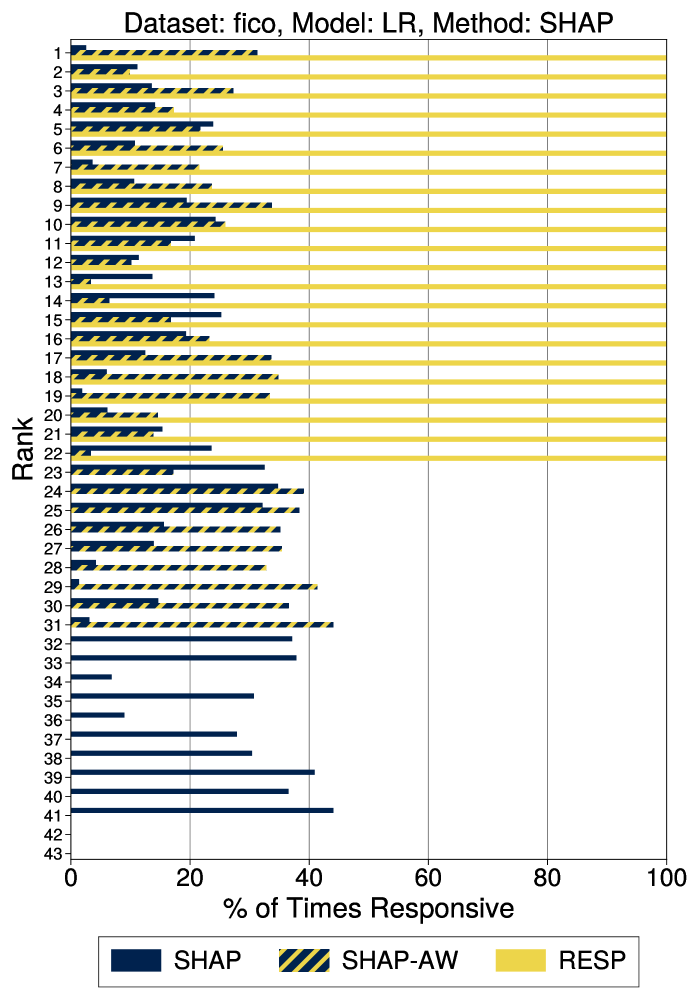
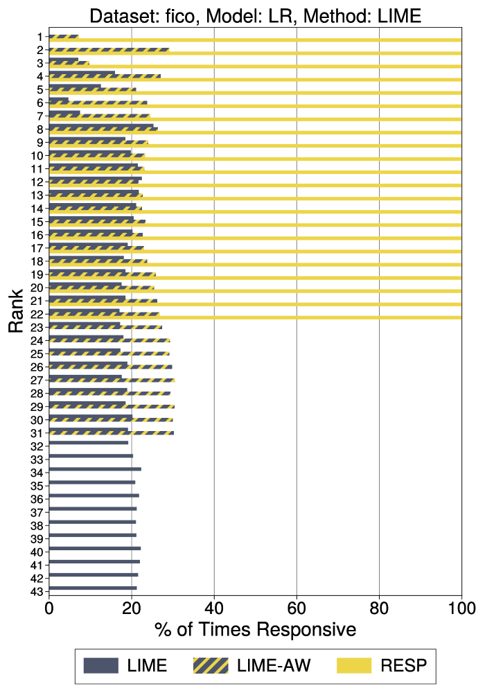
Figure 4: The percent of times where the feature at the shown rank from LIME, LIME-AW, SHAP, SHAP-AW and RESP is responsive – i.e. has at least one single-feature action that leads to recourse – for denied individuals. Only features with a non-zero score under the feature attribution method are shown. Individuals who receive a score of zero do not appear in the chart.

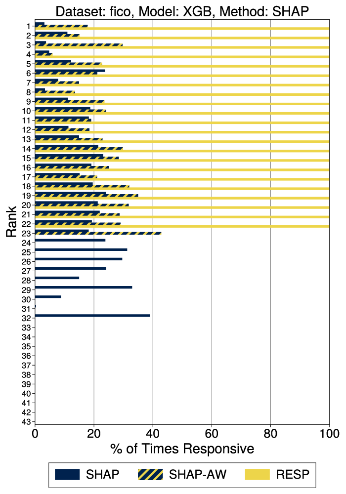
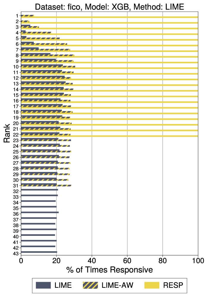
Figure 5: The percent of times where the feature at the shown rank from LIME, LIME-AW, SHAP, SHAP-AW and RESP is responsive – i.e. has at least one single-feature action that leads to recourse – for denied individuals. Only features with a non-zero score under the feature attribution method are shown. Individuals who receive a score of zero do not appear in the chart.

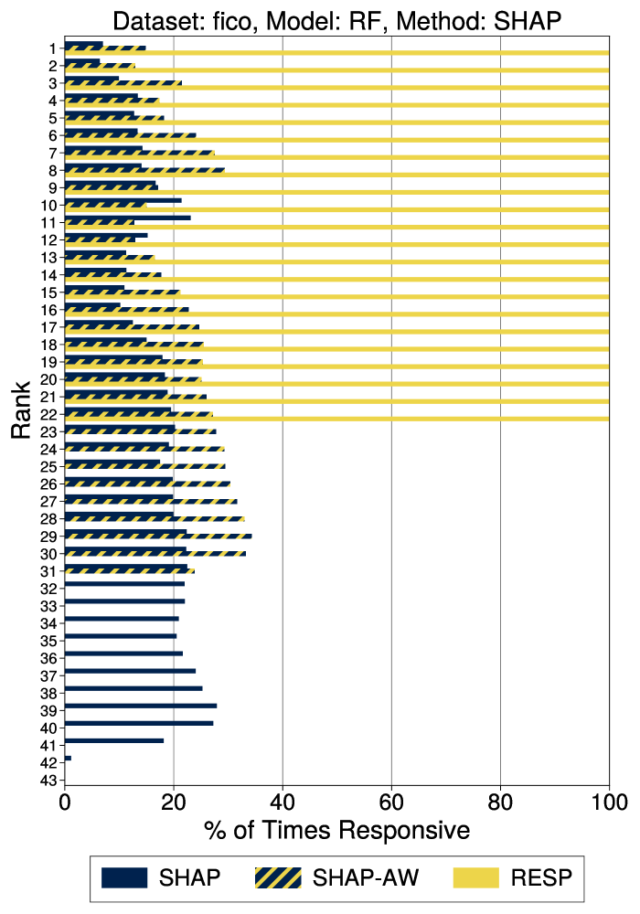
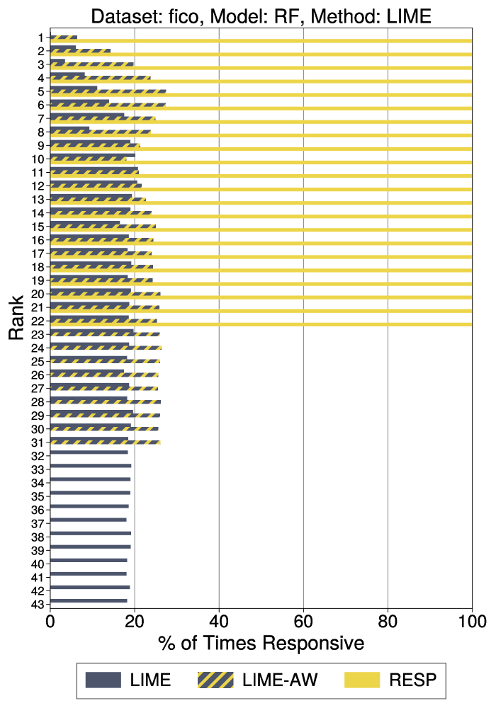
Figure 6: The percent of times where the feature at the shown rank from LIME, LIME-AW, SHAP, SHAP-AW and RESP is responsive – i.e. has at least one single-feature action that leads to recourse – for denied individuals. Only features with a non-zero score under the feature attribution method are shown. Individuals who receive a score of zero do not appear in the chart.

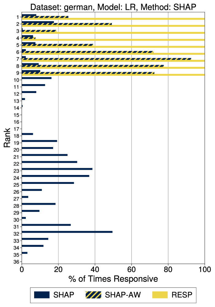
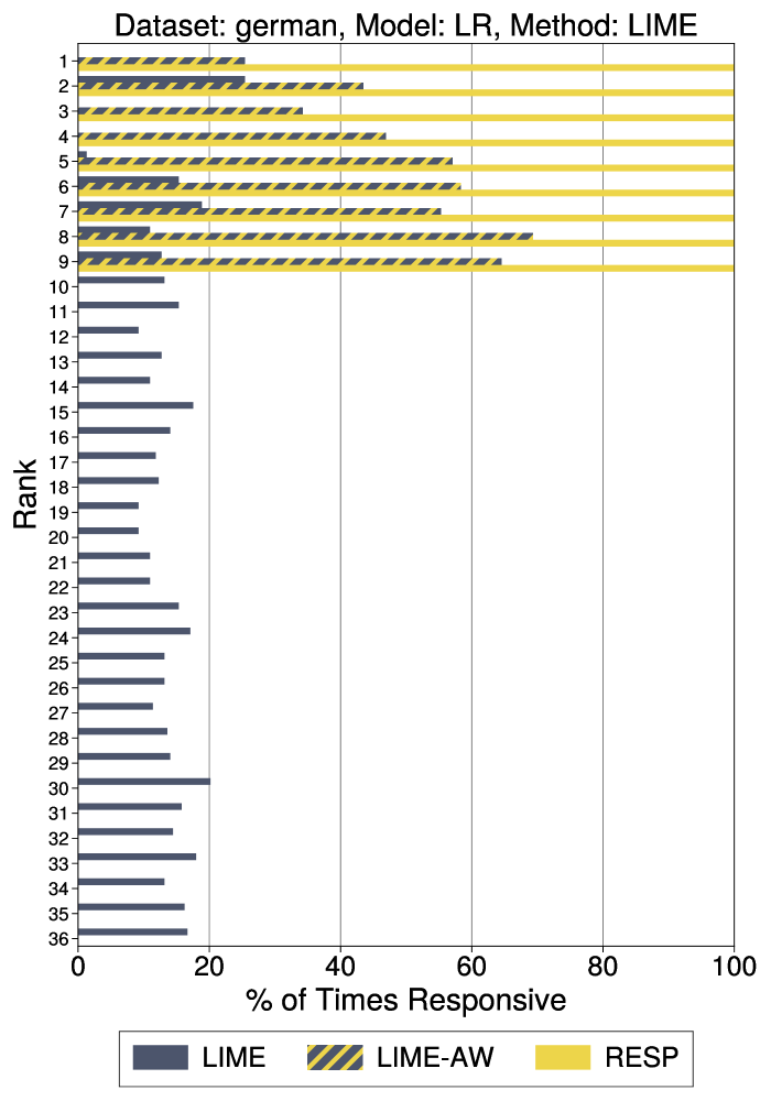
Figure 7: The percent of times where the feature at the shown rank from LIME, LIME-AW, SHAP, SHAP-AW and RESP is responsive – i.e. has at least one single-feature action that leads to recourse – for denied individuals. Only features with a non-zero score under the feature attribution method are shown. Individuals who receive a score of zero do not appear in the chart.

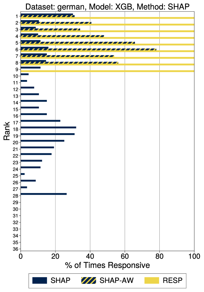
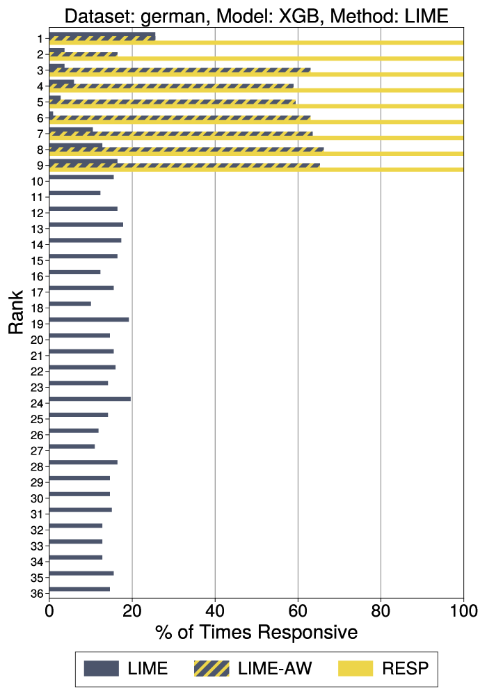
Figure 8: The percent of times where the feature at the shown rank from LIME, LIME-AW, SHAP, SHAP-AW and RESP is responsive – i.e. has at least one single-feature action that leads to recourse – for denied individuals. Only features with a non-zero score under the feature attribution method are shown. Individuals who receive a score of zero do not appear in the chart.

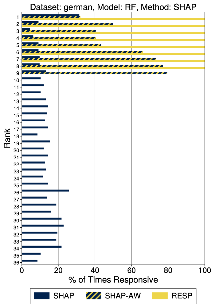
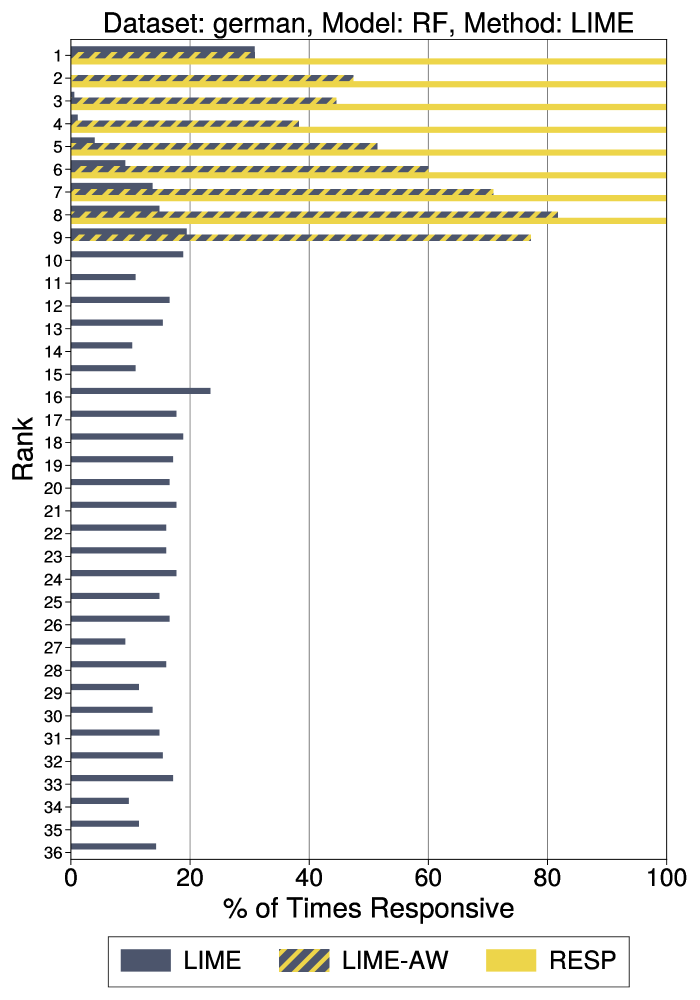
Figure 9: The percent of times where the feature at the shown rank from LIME, LIME-AW, SHAP, SHAP-AW and RESP is responsive – i.e. has at least one single-feature action that leads to recourse – for denied individuals. Only features with a non-zero score under the feature attribution method are shown. Individuals who receive a score of zero do not appear in the chart.

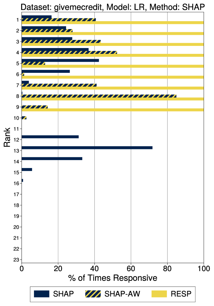
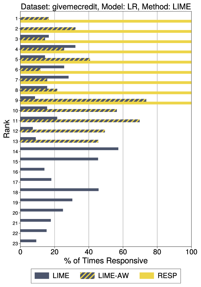
Figure 10: The percent of times where the feature at the shown rank from LIME, LIME-AW, SHAP, SHAP-AW and RESP is responsive – i.e. has at least one single-feature action that leads to recourse – for denied individuals. Only features with a non-zero score under the feature attribution method are shown. Individuals who receive a score of zero do not appear in the chart.

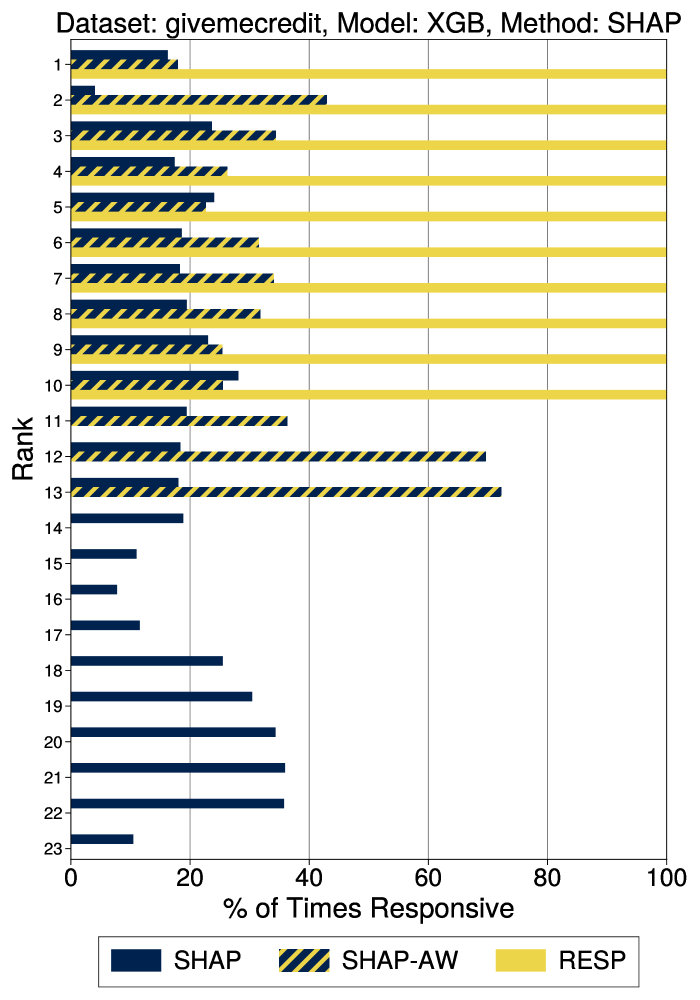
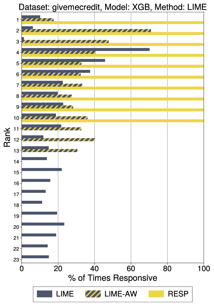
Figure 11: The percent of times where the feature at the shown rank from LIME, LIME-AW, SHAP, SHAP-AW and RESP is responsive – i.e. has at least one single-feature action that leads to recourse – for denied individuals. Only features with a non-zero score under the feature attribution method are shown. Individuals who receive a score of zero do not appear in the chart.

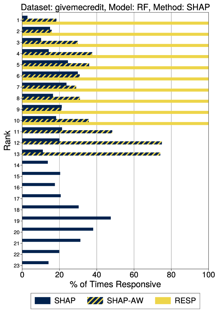
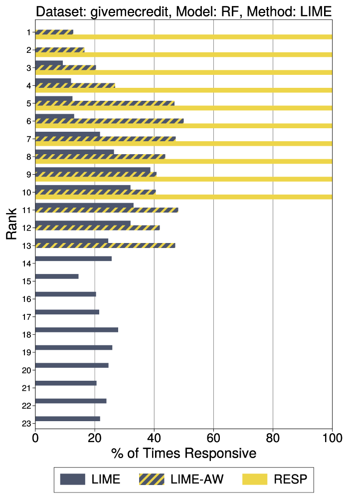
Figure 12: The percent of times where the feature at the shown rank from LIME, LIME-AW, SHAP, SHAP-AW and RESP is responsive – i.e. has at least one single-feature action that leads to recourse – for denied individuals. Only features with a non-zero score under the feature attribution method are shown. Individuals who receive a score of zero do not appear in the chart.

References

- cfp [a] 12 cfr part 1002 - equal credit opportunity act (regulation b). https://www.consumerfinance.gov/rules-policy/regulations/1002/2/, a. Accessed: 2024-07-16.
- cfp [b] Comment for 1002.9 - notifications. https://www.consumerfinance.gov/rules-policy/regulations/1002/interp-9/#9-b-1-Interp-1, b. Accessed: 2024-07-16.
- Adebayo et al. [2020] Julius Adebayo, Michael Muelly, Ilaria Liccardi, and Been Kim. Debugging tests for model explanations. arXiv preprint arXiv:2011.05429, 2020.
- Adler et al. [2018] Philip Adler, Casey Falk, Sorelle A Friedler, Tionney Nix, Gabriel Rybeck, Carlos Scheidegger, Brandon Smith, and Suresh Venkatasubramanian. Auditing black-box models for indirect influence. Knowledge and Information Systems, 54:95–122, 2018.
- Aïvodji et al. [2019] Ulrich Aïvodji, Hiromi Arai, Olivier Fortineau, Sébastien Gambs, Satoshi Hara, and Alain Tapp. Fairwashing: the risk of rationalization. In International Conference on Machine Learning, pages 161–170. PMLR, 2019.
- Barocas et al. [2020] Solon Barocas, Andrew D Selbst, and Manish Raghavan. The hidden assumptions behind counterfactual explanations and principal reasons. In Proceedings of the 2020 Conference on Fairness, Accountability, and Transparency, pages 80–89, 2020.
- Bilodeau et al. [2024] Blair Bilodeau, Natasha Jaques, Pang Wei Koh, and Been Kim. Impossibility theorems for feature attribution. Proceedings of the National Academy of Sciences, 121(2):e2304406120, 2024.
- Black et al. [2022] Emily Black, Manish Raghavan, and Solon Barocas. Model multiplicity: Opportunities, concerns, and solutions. In Proceedings of the 2022 ACM Conference on Fairness, Accountability, and Transparency, pages 850–863, 2022.
- Bogen and Rieke [2018] Miranda Bogen and Aaron Rieke. Help wanted: An examination of hiring algorithms, equity, and bias. Upturn, December, 7, 2018.
- Brown et al. [2001] Lawrence D Brown, T Tony Cai, and Anirban DasGupta. Interval estimation for a binomial proportion. Statistical science, 16(2):101–133, 2001.
- Brunet et al. [2022] Marc-Etienne Brunet, Ashton Anderson, and Richard Zemel. Implications of model indeterminacy for explanations of automated decisions. Advances in Neural Information Processing Systems, 35:7810–7823, 2022.
- De Toni et al. [2022] Giovanni De Toni, Paolo Viappiani, Stefano Teso, Bruno Lepri, and Andrea Passerini. Personalized algorithmic recourse with preference elicitation. arXiv preprint arXiv:2205.13743, 2022.
- Dominguez-Olmedo et al. [2022] Ricardo Dominguez-Olmedo, Amir H Karimi, and Bernhard Schölkopf. On the adversarial robustness of causal algorithmic recourse. In International Conference on Machine Learning, pages 5324–5342. PMLR, 2022.
- Dua and Graff [2017] Dheeru Dua and Casey Graff. UCI machine learning repository, 2017. URL http://archive.ics.uci.edu/ml.
- Edwards and Veale [2017] Lilian Edwards and Michael Veale. Slave to the algorithm: Why a right to an explanation is probably not the remedy you are looking for. Duke L. & Tech. Rev., 16:18, 2017.
- ElShawi et al. [2019] Radwa ElShawi, Youssef Sherif, Mouaz Al-Mallah, and Sherif Sakr. Ilime: local and global interpretable model-agnostic explainer of black-box decision. In Advances in Databases and Information Systems: 23rd European Conference, ADBIS 2019, Bled, Slovenia, September 8–11, 2019, Proceedings 23, pages 53–68. Springer, 2019.
- Esfahani et al. [2024] Seyedehdelaram Esfahani, Giovanni De Toni, Bruno Lepri, Andrea Passerini, Katya Tentori, and Massimo Zancanaro. Exploiting preference elicitation in interactive and user-centered algorithmic recourse: An initial exploration. arXiv preprint arXiv:2404.05270, 2024.
- Eubanks [2018] Virginia Eubanks. Automating inequality: How high-tech tools profile, police, and punish the poor. St. Martin’s Press, 2018.
- [19] Council of the European Union European Parliament. Regulation (eu) 2024/1689. https://eur-lex.europa.eu/eli/reg/2024/1689/oj. Accessed: 2024-08-30.
- FICO [2018] FICO. Explainable machine learning challenge, 2018. URL https://community.fico.com/s/explainable-machine-learning-challenge.
- FinRegLab [2023] FinRegLab. Empirical white paper: Explainability and fairness: Insights from consumer lending. Technical report, FinRegLab, July 2023. URL https://finreglab.org/wp-content/uploads/2023/12/FinRegLab_2023-07-13_Empirical-White-Paper_Explainability-and-Fairness_Insights-from-Consumer-Lending.pdf.
- Fokkema et al. [2023] Hidde Fokkema, Rianne De Heide, and Tim Van Erven. Attribution-based explanations that provide recourse cannot be robust. Journal of Machine Learning Research, 24(360):1–37, 2023.
- Fumagalli et al. [2024] Fabian Fumagalli, Maximilian Muschalik, Patrick Kolpaczki, Eyke Hüllermeier, and Barbara Hammer. Shap-iq: Unified approximation of any-order shapley interactions. Advances in Neural Information Processing Systems, 36, 2024.
- Galhotra et al. [2021] Sainyam Galhotra, Romila Pradhan, and Babak Salimi. Explaining black-box algorithms using probabilistic contrastive counterfactuals. In Proceedings of the 2021 International Conference on Management of Data, pages 577–590, 2021.
- Gilman [2020] Michele E Gilman. Poverty lawgorithms: A poverty lawyer’s guide to fighting automated decision-making harms on low-income communities. Data & Society, 2020.
- Goethals et al. [2023] Sofie Goethals, David Martens, and Theodoros Evgeniou. Manipulation risks in explainable ai: The implications of the disagreement problem. arXiv preprint arXiv:2306.13885, 2023.
- Hurley and Adebayo [2016] Mikella Hurley and Julius Adebayo. Credit scoring in the era of big data. Yale JL & Tech., 18:148, 2016.
- Jethani et al. [2021] Neil Jethani, Mukund Sudarshan, Ian Connick Covert, Su-In Lee, and Rajesh Ranganath. Fastshap: Real-time shapley value estimation. In International conference on learning representations, 2021.
- Kaggle [2011] Kaggle. Give Me Some Credit. http://www.kaggle.com/c/GiveMeSomeCredit/, 2011.
- Karimi et al. [2020a] Amir-Hossein Karimi, Gilles Barthe, Borja Balle, and Isabel Valera. Model-agnostic counterfactual explanations for consequential decisions. In International Conference on Artificial Intelligence and Statistics, pages 895–905. PMLR, 2020a.
- Karimi et al. [2020b] Amir-Hossein Karimi, Julius Von Kügelgen, Bernhard Schölkopf, and Isabel Valera. Algorithmic recourse under imperfect causal knowledge: a probabilistic approach. Advances in neural information processing systems, 33:265–277, 2020b.
- Karimi et al. [2021a] Amir-Hossein Karimi, Gilles Barthe, Bernhard Schölkopf, and Isabel Valera. A survey of algorithmic recourse: definitions, formulations, solutions, and prospects. 2021a.
- Karimi et al. [2021b] Amir-Hossein Karimi, Bernhard Schölkopf, and Isabel Valera. Algorithmic recourse: from counterfactual explanations to interventions. In Proceedings of the 2021 ACM Conference on Fairness, Accountability, and Transparency, FAccT ’21, pages 353–362, New York, NY, USA, 2021b. Association for Computing Machinery. ISBN 9781450383097. doi: 10.1145/3442188.3445899. URL https://doi.org/10.1145/3442188.3445899.
- Kaur et al. [2020] Harmanpreet Kaur, Harsha Nori, Samuel Jenkins, Rich Caruana, Hanna Wallach, and Jennifer Wortman Vaughan. Interpreting interpretability: understanding data scientists’ use of interpretability tools for machine learning. In Proceedings of the 2020 CHI conference on human factors in computing systems, pages 1–14, 2020.
- Koh et al. [2024] Seunghun Koh, Byung Hyung Kim, and Sungho Jo. Understanding the user perception and experience of interactive algorithmic recourse customization. ACM Transactions on Computer-Human Interaction, 2024.
- Kothari et al. [2024] Avni Kothari, Bogdan Kulynych, Tsui-Wei Weng, and Berk Ustun. Prediction without preclusion: Recourse verification with reachable sets. In The Twelfth International Conference on Learning Representations, 2024. URL https://openreview.net/forum?id=SCQfYpdoGE.
- Kulesza et al. [2015] Todd Kulesza, Margaret Burnett, Weng-Keen Wong, and Simone Stumpf. Principles of explanatory debugging to personalize interactive machine learning. In Proceedings of the 20th international conference on intelligent user interfaces, pages 126–137, 2015.
- Lakkaraju and Bastani [2020] Himabindu Lakkaraju and Osbert Bastani. "how do i fool you?": Manipulating user trust via misleading black box explanations. In Proceedings of the AAAI/ACM Conference on AI, Ethics, and Society, AIES ’20, pages 79–85, New York, NY, USA, 2020. Association for Computing Machinery. ISBN 9781450371100. doi: 10.1145/3375627.3375833. URL https://doi.org/10.1145/3375627.3375833.
- Lei et al. [2018] Jing Lei, Max G’Sell, Alessandro Rinaldo, Ryan J Tibshirani, and Larry Wasserman. Distribution-free predictive inference for regression. Journal of the American Statistical Association, 113(523):1094–1111, 2018.
- Lundberg and Lee [2017] Scott M Lundberg and Su-In Lee. A unified approach to interpreting model predictions. NeurIPS, 2017.
- Marx et al. [2019] Charles Marx, Richard Phillips, Sorelle Friedler, Carlos Scheidegger, and Suresh Venkatasubramanian. Disentangling influence: Using disentangled representations to audit model predictions. Advances in Neural Information Processing Systems, 32, 2019.
- Marx et al. [2020] Charles Marx, Flavio Calmon, and Berk Ustun. Predictive multiplicity in classification. In Proceedings of Machine Learning and Systems 2020, pages 9215–9224. 2020.
- Mothilal et al. [2020] Ramaravind K Mothilal, Amit Sharma, and Chenhao Tan. Explaining machine learning classifiers through diverse counterfactual explanations. In Proceedings of the 2020 conference on fairness, accountability, and transparency, pages 607–617, 2020.
- Nguyen et al. [2023] Duy Nguyen, Ngoc Bui, and Viet Anh Nguyen. Distributionally robust recourse action. arXiv preprint arXiv:2302.11211, 2023.
- Pawelczyk et al. [2023] Martin Pawelczyk, Teresa Datta, Johan Van den Heuvel, Gjergji Kasneci, and Himabindu Lakkaraju. Probabilistically robust recourse: Navigating the trade-offs between costs and robustness in algorithmic recourse. In The Eleventh International Conference on Learning Representations, 2023.
- Raghavan et al. [2020] Manish Raghavan, Solon Barocas, Jon Kleinberg, and Karen Levy. Mitigating bias in algorithmic hiring: Evaluating claims and practices. In Proceedings of the 2020 conference on fairness, accountability, and transparency, pages 469–481, 2020.
- Ribeiro et al. [2016] Marco Tulio Ribeiro, Sameer Singh, and Carlos Guestrin. Why should I trust you?: Explaining the predictions of any classifier. In Proceedings of the 22nd ACM SIGKDD International Conference on Knowledge Discovery and Data Mining, pages 1135–1144. ACM, 2016.
- Ribeiro et al. [2018] Marco Tulio Ribeiro, Sameer Singh, and Carlos Guestrin. Anchors: High-precision model-agnostic explanations. In AAAI Conference on Artificial Intelligence, 2018.
- Selbst and Barocas [2018] Andrew D Selbst and Solon Barocas. The intuitive appeal of explainable machines. 2018.
- Shapley [1953] Lloyd S Shapley. A value for n-person games. Contribution to the Theory of Games, 2, 1953.
- Slack et al. [2020] Dylan Slack, Sophie Hilgard, Emily Jia, Sameer Singh, and Himabindu Lakkaraju. Fooling lime and shap: Adversarial attacks on post hoc explanation methods. In Proceedings of the AAAI/ACM Conference on AI, Ethics, and Society, pages 180–186, 2020.
- Slack et al. [2021] Dylan Slack, Anna Hilgard, Himabindu Lakkaraju, and Sameer Singh. Counterfactual explanations can be manipulated. Advances in neural information processing systems, 34:62–75, 2021.
- Taylor [1980] Winnie F Taylor. Meeting the equal credit opportunity act’s specificity requirement: Judgmental and statistical scoring systems. Buff. L. Rev., 29:73, 1980.
- The Lawyers’ Committee for Civil Rights Under Law [December, 2023] The Lawyers’ Committee for Civil Rights Under Law. Online civil rights act, December, 2023. URL https://www.lawyerscommittee.org/online-civil-rights-act.
- Union [2024] European Union. Regulation (eu) 2024/1689: Artificial intelligence act. https://www.aiact-info.eu/article-86-right-to-explanation-of-individual-decision-making/, 2024. Accessed: 2024-08-01.
- Upadhyay et al. [2021] Sohini Upadhyay, Shalmali Joshi, and Himabindu Lakkaraju. Towards robust and reliable algorithmic recourse. arXiv preprint arXiv:2102.13620, 2021.
- Ustun et al. [2019] Berk Ustun, Alexander Spangher, and Yang Liu. Actionable recourse in linear classification. In Proceedings of the Conference on Fairness, Accountability, and Transparency, FAT* ’19, pages 10–19. ACM, 2019. ISBN 978-1-4503-6125-5. doi: 10.1145/3287560.3287566.
- von Kügelgen et al. [2022] Julius von Kügelgen, Amir-Hossein Karimi, Umang Bhatt, Isabel Valera, Adrian Weller, and Bernhard Schölkopf. On the fairness of causal algorithmic recourse. In Proceedings of the AAAI Conference on Artificial Intelligence, volume 36, pages 9584–9594, 2022.
- Watson-Daniels et al. [2023] Jamelle Watson-Daniels, David C. Parkes, and Berk Ustun. Predictive multiplicity in probabilistic classification. In AAAI Conference on Artificial Intelligence, 06 2023.
- White House [October, 2022] White House. Blueprint for an AI bill of rights: Making automated systems work for the American people. The White House Office of Science and Technology Policy, October, 2022. URL https://www.whitehouse.gov/ostp/ai-bill-of-rights/.
- Wolsey [2020] Laurence A Wolsey. Integer programming. John Wiley & Sons, 2020.
- Wykstra [2020] S Wykstra. Government’s use of algorithm serves up false fraud charges. undark, 6 january, 2020.
- Zafar and Khan [2019] Muhammad Rehman Zafar and Naimul Mefraz Khan. Dlime: A deterministic local interpretable model-agnostic explanations approach for computer-aided diagnosis systems. arXiv preprint arXiv:1906.10263, 2019.
- Zhou et al. [2022] Yilun Zhou, Serena Booth, Marco Tulio Ribeiro, and Julie Shah. Do feature attribution methods correctly attribute features? In Proceedings of the AAAI Conference on Artificial Intelligence, volume 36, pages 9623–9633, 2022.
- Zhou et al. [2021] Zhengze Zhou, Giles Hooker, and Fei Wang. S-lime: Stabilized-lime for model explanation. In Proceedings of the 27th ACM SIGKDD conference on knowledge discovery & data mining, pages 2429–2438, 2021.