FGCE: Feasible Group Counterfactual Explanations for Auditing Fairness

Abstract

This paper introduces the first graph-based framework for generating group counterfactual explanations to audit model fairness, a crucial aspect of trustworthy machine learning. Counterfactual explanations are instrumental in understanding and mitigating unfairness by revealing how inputs should change to achieve a desired outcome. Our framework, named Feasible Group Counterfactual Explanations (FGCEs), captures real-world feasibility constraints and constructs subgroups with similar counterfactuals, setting it apart from existing methods. It also addresses key trade-offs in counterfactual generation, including the balance between the number of counterfactuals, their associated costs, and the breadth of coverage achieved. To evaluate these trade-offs and assess fairness, we propose measures tailored to group counterfactual generation. Our experimental results on benchmark datasets demonstrate the effectiveness of our approach in managing feasibility constraints and trade-offs, as well as the potential of our proposed metrics in identifying and quantifying fairness issues.

I Introduction

AI-driven technologies increasingly influence various aspects of society shaping significant decisions that impact our lives. Ensuring the fairness of their decisions and providing a clear understanding of why they yield specific outputs is becoming a societal imperative. Various types of explanation methods have emerged for providing transparency of such decisions  [1, 2, 3, 4]. Among them, counterfactual explanations (CFEs) have attracted significant attention [5]. CFEs offer insights into how altering the features of an instance could lead to a different outcome for this instance.

While most previous work focuses on CFEs for individual instances [6, 7, 8, 9, 10], there is increasing interest in group counterfactuals (GCEs). Unlike individual CFEs, which alter features for single instances, GCFEs explore how modifying features can impact entire groups. This approach is particularly valuable in real-world applications such as fairness in lending, hiring, and criminal justice, where decisions affect groups collectively. GCFEs help assess and gain insights into unfairness by revealing how different changes in features might influence outcomes across different groups [11, 12, 13]. However, existing methods often fall short of producing GCFEs that are feasible and actionable. GCFEs should be coherent with the data distribution, representative of the population, and propose feasible feature alterations.

In this paper, we introduce Feasible Group Counterfactual Explanations (FGCE), a novel graph-based approach to generating group counterfactuals. Our approach utilizes a density-weighted graph that encapsulates feasibility constraints [6]. We call this graph feasibility graph. The graph facilitates feasible transformations between instances while considering the associated costs of these transformations. We represent feasibility through reachability in the feasibility graph. The connected components of the graph represent subgroups of the group to be explained, which are covered by the same set of counterfactuals.

We propose efficient algorithms for identifying a small set of counterfactuals that cover many instances in the group (i.e., are feasible transformations) and capture the various trade-offs in group counterfactual generation. FGCE ensures that the generated CFEs are aligned with the underlying data distribution and offers practical and feasible insights for the decision-making process.

Then, we use FGCE to explain and measure unfairness. Specifically, we consider groups of instances defined based on the value of one or more of their sensitive attributes, and generate FGCEs for each group. We introduce novel measures of the fairness of each group by comparing the FGCEs of each group. Our measures encapsulate the trade-offs of the size, coverage, and cost of the FGCEs and are applicable at both the group and the subgroup level.

Finally, we present experimental results of the fairness of three real datasets using the proposed metrics that show the effectiveness of FGCE in auditing unfairness. We also compare experimentally our method with related research. Despite incorporating stringent feasibility constraints, our method outperforms existing baselines, demonstrating its ability to propose counterfactuals that align with the underlying data distribution.

The remainder of this paper is structured as follows. In Section 2, we introduce the problem, in Section 3 our algorithms, and in Section 4, the FGCE-based fairness measures. In Section 5, we present experimental results, in Section 6 related work, and in Section 7, we offer conclusions.

II Problem Definition

We consider a binary classifier $f:\mathbb{R}^{d}\rightarrow\{0,1\}$, which maps instances in a $d$-dimensional feature space into two classes, labeled 0 and 1. Let $U\subseteq\ \mathbb{R}^{d}$ denote the input space. A model prediction on an individual instance $\mathbf{x}$ $\in$ $U$, called factual, is explained by crafting a counterfactual (CF) instance $\mathbf{x’}$ $\in$ $\mathbb{R}^{d}$ that is similar to $\mathbf{x}$ but its outcome $f(\mathbf{x^{\prime}})$ differs from the initial prediction $f(\mathbf{x})$ [5]. The changes in feature values from $\mathbf{x}$ to $\mathbf{x’}$ should be feasible, adhering to real-world constraints. For instance, alterations to immutable features, such as race or height, should be prohibited. Formally, a CF $\mathbf{x^{\prime}}$ for $\mathbf{x}$ is defined as: $\mathbf{x}^{\prime}={\mathrm{arg}}\ {\mathrm{min_{\mathbf{x}^{\prime}\in{A}_{x}}}\ cost(\mathbf{x},\mathbf{x}^{\prime})\,\text{s.t.}\,f(\mathbf{x}^{\prime})\neq f(\mathbf{x})},$ where $cost(\mathbf{x},\mathbf{x}^{\prime})$ is a distance function and ${A}_{x}$ restricts the set of counterfactuals to those attainable from $\mathbf{x}$ through feasible changes.

Counterfactuals not only explain a decision but also suggest the actions to be applied to a factual for getting a favorable outcome. For example, consider a classifier that decides whether a person is eligible for a loan, using features such as age, education, or income. Say Alice is refused the loan. A counterfactual for Alice could for example indicate that Alice should have received the loan, if she had a MSc degree, or her income was increased by 10K.

It would be hard to trust a counterfactual if it resulted in a combination of features that were unlike any observations the classifier has seen before [5], thus counterfactuals should also be coherent with the underlying data distribution. To ensure feasibility and trustworthiness, we adopt a graph-based approach. We construct a weighted directed graph $G_{U}=(V,E,W)$, termed feasibility graph, whose nodes correspond to instances in $U$ and there is an edge between nodes $\mathbf{x_{i}}$ and $\mathbf{x_{j}}$, if changes between the corresponding instances meet feasibility constraints and the distance between them falls within a predetermined threshold denoted as $\epsilon$. This ensures that alterations between instances are both feasible and small. The weight function $W$ is defined following the density-based approach introduced in FACE [6] to ensure that counterfactuals lie in dense areas of the input space and avoid outliers. Each edge in $G_{U}$ is assigned a weight $W_{ij}$, calculated as the product of the distance between the instances (capturing the difficulty of transitioning) and the density of the instances around the midpoint of $\mathbf{x_{i}}$ and $\mathbf{x_{j}}$, where density is estimated using a Kernel Density Estimator (KDE) [14] :

$$W_{ij} =KDE\left(\frac{\mathbf{x_{i}}+\mathbf{x_{j}}}{2}\right)\|\mathbf{x_{i}}-\mathbf{x_{j}}\|$$

Given a feasibility graph $G_{U}$, we define the feasibility set $A_{\mathbf{x}}$ of instance $\mathbf{x}$ to be the set of instances $\mathbf{x}^{\prime}$ for which there is a path in $G_{U}$ from $\mathbf{x}$ to $\mathbf{x}^{\prime}$, i.e., the set of instances that are reachable from $\mathbf{x}$: $A_{\mathbf{x}}=\{\mathbf{x}^{\prime}\in\mathbf{U}|\mathbf{x}^{\prime}$ is reachable from $\mathbf{x}\text{ in }G_{U}\}$. We call instances in this set feasible counterfactuals for $\mathbf{x}$.

In this paper, instead of finding a CF for a single instance $\mathbf{x}$, we are interested in providing counterfactuals for a set $X\subseteq U$ of instances mapped to the same class. Let $X^{\prime}\subseteq U$ be the set of instances mapped to the opposite class. Our goal is to identify a small subset $S$ of $X^{\prime}$ of size $k$ that best explains $X$. We constrain the number $k$ of CFs for interpretability, so that the produced CFs are manageable. To select $S$, we consider the trade-off between coverage and cost.

For a group of counterfactuals $S\subseteq X^{\prime}$, coverage is defined as:

$coverage(X,S)=\left|\{\mathbf{x}\,|\,\mathbf{x}\in X\text{ and }\exists\text{ }\mathbf{x^{\prime}}\in S\cap A_{\mathbf{x}}\}\right|$

We overload notation and use function $cost$ to define both the cost between an instance and a set of instances and the cost between two sets of instances as follows:

$$cost(\mathbf{x},S)=\min_{\mathbf{x}^{\prime}\in S}cost(\mathbf{x},\mathbf{x}^{\prime}),$$

$$cost(X,S)=\min\max_{\mathbf{x}\in X}cost(\mathbf{x},S)$$

The cost function $cost(\mathbf{x},\mathbf{x^{\prime}})$ between two instances $\mathbf{x}$ and $\mathbf{x^{\prime}}$ can be any function that captures the cost of transforming $\mathbf{x}$ to $\mathbf{x^{\prime}}$ offering flexibility to adapt to specific problem requirements. For example, cost can be defined as the vector distance (e.g., L2 distance) between $\mathbf{x}$ and $\mathbf{x}^{\prime}$. Alternatively, cost can be defines as the sum of edge weights along the shortest path from $\mathbf{x}$ to $\mathbf{x}^{\prime}$ in the feasibility graph, or as the number of hops on this path. By emphasizing proximity in feature space and considering dense paths, these definitions ensure that the derived counterfactual explanations are both feasible and closely aligned with real data instances. Our approach works with any definition of cost.

We provide two definitions of the Feasible Group Counterfactual Explanation (FGCE) problem. Our first definition prioritizes cost over coverage setting a threshold on cost.

Problem 1 (Cost-Constrained FGCE)

Given $X$, $X^{\prime}$, $k$ $\in\mathbb{N}_{*}$, and distance threshold $d\in\mathbb{R}_{*}^{+}$, find $S\subseteq X^{\prime}$ with $|S|\leq k$ and $Q\subseteq X$ such that for every instance $\mathbf{x}\in Q$ there exist an instance $\mathbf{x}^{\prime}\in S$ such that $cost(\mathbf{x},\mathbf{x}^{\prime})\leq d$ and $|Q|$ is maximized.

Our second problem definition prioritizes coverage over cost, asking for a set that provides a specified coverage degree $c$.

Problem 2 (Coverage-Constrained FGCEs)

Given $X$, $X^{\prime}$, $k$ $\in\mathbb{N}_{*}$, and coverage degree $c$, $0<c\leq 1$, find $S\subseteq X^{\prime}$ with $|S|\leq k$ such that $coverage(X,S)\geq c\,|X|$ and $cost(X,S)$ is minimized.

III Algorithms

Our approach to generating feasible counterfactuals hinges on the feasibility graph $G_{U}$ that inherently captures the dataset constraints. It is easy to see that a necessary condition for $\mathbf{x}^{\prime}$ to be a feasible counterfactual for $\mathbf{x}$ is that $\mathbf{x}$ and $\mathbf{x}^{\prime}$ belong to same weakly connected component (WCC) of $G_{U}$. Thus, $G_{U}$ splits the set of factuals $X$ into $m$, $m>0$, disjoint subsets $X_{i}$, where each $X_{i}$ includes the instances of $X$ that belong to the same WCC of $G_{U}$ and whose feasible counterfactuals are also disjoint subsets $X^{\prime}_{i}$ belonging to the same WCC with $X_{i}$. This partition of $X$ into $m$ subgroups with distinct feasible explanations offers an opportunity to understand the behavior of the model both at the group and at the subgroup level.

In the following, we present two versions: (a) a global version that generates counterfactuals for the whole set $X$ and (b) a local version that generates counterfactuals per subgroup $X_{i}$. We also show how the local version can be used to generate counterfactuals for the whole group $X$.

III-A Cost-Constrained FGCE

We formulate the global version of the cost-constrained problem as a greedy optimization problem, where we maximize coverage by iteratively selecting counterfactuals that cover the maximum number of factual instances from $X$ that have not yet been covered (Algorithm 1). In Lines 2-4, we compute for each candidate counterfactual $\mathbf{x}’$ the number of factuals covered by it. The greedy selection is then applied to these candidates to determine the final set $S$ of counterfactuals.

Algorithm 1 Global Greedy

0:  Feasibility graph $G_{U}$, set $X$, number $k$ of CFs, cost threshold $d$.

0:  A set $S\subseteq X^{\prime}$ of cost-constrained FGCEs.

1:  $S\leftarrow\emptyset$; $Covered\leftarrow\emptyset$

2:   $A_{X}$ $\leftarrow$ $\cup_{\mathbf{x}\in X}A_{x}$

3:  for $\mathbf{x}^{\prime}$ $\in$ $A_{X}$ do

4:    $Cov[\mathbf{x}^{\prime}]$ $\leftarrow$ $\{\mathbf{x}|\mathbf{x}\in X\,\text{and}\,\,cost(\mathbf{x},\mathbf{x}^{\prime})\leq d\}$

5:  while $|S|<k$ and $|Covered|$ $<|X|$

6:   $\mathbf{x}^{\prime}$ $\leftarrow$ $\arg\max_{\mathbf{y}\in A_{X}}|Cov[y]-Covered|$

7:   $S\leftarrow S\cup\{\mathbf{x}^{\prime}\}$

8:   $Covered\leftarrow Covered\cup Cov[\mathbf{x}^{\prime}]$

9:  return $S$

The complexity of Algorithm 1 depends on the cost function. To find feasible counterfactuals, i.e., ensure the reachability requirement (Line 2), we use Breadth-First-Search which results in $O(|V|+|E|)$ complexity. In case of the cost function being the vector distance, computing covered instances in Line 4 takes $O(|X|)$, while in case of shortest path distances it takes time $O(|V|\text{log}(|V|)+|E|)$ using Dijkstra’s Algorithm. This step is repeated at most $|X^{\prime}|$ times.

Given the submodular nature of our coverage function, where the marginal gain of adding a new CF to the set $S$ decreases as $S$ grows, Algorithm 1 adheres to the properties of submodular maximization. Consequently, the attained coverage is no worse than $(1-\frac{1}{e})$ times the optimal maximum coverage [15].

Algorithm 1 can also be used to provide a counterfactual explanation for a subgroup $X_{i}$ by applying it only to the corresponding WCC. We can also utilize this local version to provide counterfactuals for the whole group $X$ by applying the greedy algorithm iteratively to all $m$ WCC as follows. Initially, we apply a single step of the greedy algorithm at each WCC. Then we select the CF that provides the overall best coverage and apply an additional step of the algorithm to the WCC from where the CF was selected. We repeat this until the maximum number $k$ of counterfactuals is reached or all factual instances are covered. It is easy to see that this local version provides the same result as the global one.

III-B Coverage-Constrained FGCE

The coverage-constrained FGCE problem is similar to the classical $k$-center problem that is known to be NP-hard  [16]. While there are known polynomial 2-approximations for this problem, in this paper, we adopt a mixed integer programming (MIP) formulation which proves to be very efficient in practice  [17]. Let $r_{\mathbf{x}\mathbf{x}^{\prime}}=1$ if $\mathbf{x}^{\prime}$ covers $\mathbf{x}$; and $r_{\mathbf{x}\mathbf{x}^{\prime}}=0$, otherwise. Let $u_{\mathbf{x}^{\prime}}=1$ if counterfactual $\mathbf{x}^{\prime}$ covers any instance in $X$, and $u_{\mathbf{x}^{\prime}}=0$ otherwise. The goal is to minimize the maximum cost $d$ of the farthest instance, while ensuring $coverage(X,S)\geq c\,|X|$:

$$\text{minimize }d$$

$$\sum_{\mathbf{x}^{\prime}\in X^{\prime}}cost(\mathbf{x},\mathbf{x}^{\prime})r_{\mathbf{x}\mathbf{x}^{\prime}}\leq d,\;\;\forall\mathbf{x}\in X$$ (1)

$$\sum_{\mathbf{x}^{\prime}\in X^{\prime}}r_{\mathbf{x}\mathbf{x}^{\prime}}\leq 1,\;\;\forall\mathbf{x}\in X$$ (2)

$$\sum_{\mathbf{x}^{\prime}\in X^{\prime}}u_{\mathbf{x}^{\prime}}\leq k$$ (3)

$$r_{\mathbf{x}\mathbf{x}^{\prime}}\leq u_{\mathbf{x}^{\prime}},\;\;\forall\mathbf{x}^{\prime}\in X^{\prime}\;\text{ and }\forall\mathbf{x}\in X$$ (4)

$$\sum_{\mathbf{x}^{\prime}\in X^{\prime}}\sum_{\mathbf{x}\in X}r_{\mathbf{x}\mathbf{x}^{\prime}}\geq c\,|X|$$ (5)

$$u_{x},r_{\mathbf{x}\mathbf{x}^{\prime}}\in\{0,1\},\quad\forall\mathbf{x}\in X,\mathbf{x}^{\prime}\in X^{\prime}$$ (6)

Constraint 1 establishes that cost $d$ must be the maximum of the pairwise costs. Constraint 2 ensures that the sum of the $r_{\mathbf{x}\mathbf{x}^{\prime}}$ variables over $\mathbf{x}^{\prime}$ is at most 1. Constraint 3 limits the number of selected instances $\mathbf{x}^{\prime}\in X^{\prime}$ at $k$. Constraint 4 specifies that if $u_{\mathbf{x}^{\prime}}=1$ (instance $\mathbf{x}^{\prime}$ covers at least one instance $\mathbf{x}$) then instances $\mathbf{x}^{\prime}\in X^{\prime}$ for which $r_{\mathbf{x}\mathbf{x}^{\prime}}=1$ should assigned to them. Constraint 5 ensures that the desired coverage percentage is achieved. Finally, Constraint 6 imposes binary restrictions. Note that for full coverage, i.e, $c=1$, Constraint 2 becomes an equality constraint, and Constraint 5 is unnecessary.

In the global version, we invoke the MIP algorithm on the $G_{U}$ graph. To improve performance, we add constraints only for instances $\mathbf{x}$ and $\mathbf{x}^{\prime}$, such that $\mathbf{x}^{\prime}\in A_{X}$. In the local version, to get counterfactuals for a specific subgroup $X_{i}$ of $X$, we invoke the MIP algorithm at the corresponding WCC of $G_{U}$.

We now describe how the local version can be applied to solve the global version. Let us first consider the simplest case of full coverage, i.e., $c=1$. Suppose we have $m$ WCCs ordered arbitrarily as $C_{1},C_{2},\ldots,C_{m}$. In this case, achieving full coverage simplifies to distributing $k$ counterfactuals among these $m$ components. Note that the maximum number of counterfactuals that can be allocated to each WCC is at most $k-m$, since for full coverage we need at least one counterfactual per WCC. First, we run MIP at each WCC with $k$ varying from 1 up to $k-m$. Let $l_{i}$ denote the minimum number of counterfactuals needed to fully cover the $i$-th WCC. We start by allocating $l_{i}$ counterfactuals to each $C_{i}$. Next, we keep allocating one counterfactual at a time to the component with the highest cost until the total number of allocated counterfactuals equals $k$.

When $c<1$, the task becomes more complex as we have to allocate both $k$ and coverage $c$ across the WCCs. Let $F({1...i},k,n)$ be the minimum cost of allocating $k$ counterfactuals that cover a total of $n$ factuals considering connected components $C_{1},....,C_{i}$. Similarly, let $F(i,k,n)$ represent the minimum cost of allocating $k$ counterfactuals to cover $n$ factuals within just component $C_{i}$. Then we can solve the problem using dynamic programming as follows:

$$F({1...i},k,n)= \min_{1\leq n^{\prime}\leq n,1\leq k^{\prime}\leq k}$$

$$\left\{F({1...i-1},k-k^{\prime},n-n^{\prime})+F(i,k^{\prime},n^{\prime})\right\}$$

This dynamic programming approach has a time complexity of $O(m(kn)^{2})$, where $m$ is the number of components, $k$ is the number of counterfactuals, and $n$ $=c|X|$.

IV FGCE for Auditing Fairness

In this section, we examine algorithmic fairness through the lens of FGCEs. In a high level, group (algorithmic) fairness refers to a set of criteria aimed at ensuring that protected groups, such as those defined by the values of sensitive attributes, like gender, race, or age, are treated similarly by the classifier. These criteria can be categorized into [18]: those based on demographic parity, which require that the proportion of groups receiving favorable outcomes reflects their representation in the input, and error-based ones, which focus on equalizing classification errors, such as false negatives, across groups.

Previous research has explored counterfactual explanations towards measuring and understanding group unfairness [4]. FGCEs offer novel tools in both directions. The main idea is to generate FGCEs for each of the groups.

Let $X$ be one of the groups. We generate FGCEs for subsets of $X$, depending on the type of group fairness that we want to explore. For example, for demographic parity, we generate counterfactuals for the instances of $X$ that are classified to the negative class, while for error-based fairness, for e.g., the instances of $X$ that are falsely classified to the negative class, i.e., the false negatives. Disparities among the FGCEs generated for each of the groups can signal underlying biases warranting deeper investigation.

One of the distinctive features of FGCE is that it allows addressing fairness at multiple levels. FGCE partitions each group into subgroups based on the connected components of the feasibility graph, resulting in distinct FGCEs for each subgroup $X_{i}$. This provides a partition of $X$ into subgroups with distinct feasible explanations and offers an opportunity to understand unfair behavior both at the group and at the subgroup level.

Burden-based Fairness Measures. Counterfactuals provide a novel approach to measuring unfairness by evaluating both the disparities in outcomes between groups and the effort required by these groups to achieve fairness, i.e., to obtain a favorable outcome. This effort, also called burden, is often estimated as the aggregated cost between the factuals in a group and their counterfactuals [9, 19].

FGCE provides a set of novel measures of burden that are: (a) parameterized by the number $k$ of counterfactuals, the maximum cost $d$, and the attained coverage $c$, and (b) applicable at both the group and the subgroup level. The importance of including the number $k$ of CFs in the fairness metric is multifaced: it ensures fairness in terms of interpretability, as groups requiring fewer CFs are more interpretable; it promotes fair treatment and trust, as models that require fewer CFs for explaining a group are more transparent and reliable, and it enhances practical fairness by assessing if minimum CFs are uniformly provided across groups.

Minimum k ($k_{0}$) and cost ($d_{0}$) for full coverage. Our first measure is the pair ($k_{0}$, $d_{0}$) where $k_{0}$ is the minimum number of counterfactuals to achieve full coverage (i.e., $c$ = 1) and $d_{0}$ the minimum required cost:

$$k_{0} =\min\{k\in\mathbb{R}_{*}|\,\exists S,|S|\leq k\text{ and }coverage(X,S)=|X|\},$$

$$d_{0} =\min\{d\in\mathbb{R}_{*}^{+}|\,\exists S,cost(X,S)\leq d\text{ and }$$

$$\hskip 34.14322pt\text{coverage}(X,S)=|X|\}$$

To compute $k_{0}$ and $d_{0}$, we solve the coverage-constrained FGCE problem. Clearly, $k_{0}\geq m$, where $m$ is the number of WCCs of $G_{U}$ that include instances of $X$. These values offer insights on the minimum resources required for full coverage of all factuals in $X$.

Area under the curve and saturation points. We now introduce a family of measures to capture the trade-offs of cost, number of counterfactuals, and coverage. The AUC (area under the curve) metrics provide a holistic view of group fairness over a range of cost, number of counterfactuals, and coverage values. The measures avoid biases that might favor one group over another when focusing on a specific set of values thus ensuring a more accurate assessment.

Let $S_{k,d}$ be the set of at most $k$ counterfactuals that provides the best coverage of $X$ with cost at most $d$, and $S_{k,c}$ be the set of at most $k$ counterfactuals that provide at least $c$ coverage with the minimum cost:

$$S_{k,d} =argmax_{|S|\leq k,\,cost(X,S)\leq d}|coverage(X,S)|,$$

$$S_{k,c} =argmin_{|S|\leq k,\,coverage(X,S)\geq c\,|X|}cost(X,S)$$

We define the area under the curve for $k$, $kAUC(k)$, as:

$$kAUC(k)=\int_{d_{min}}^{d_{max}}\text{coverage}(X,S_{k,d})d{d}$$

This metric measures the area under the curve when plotting coverage over a range of cost values for a given number of counterfactuals $k$. This offers insights into how effectively a group can achieve coverage across varying costs for a given $k$. There is a value of cost that provides the largest possible coverage for $k$, we call it saturation point for $k$ and denote it as $sp(k)$. That is, it holds, for any $d\geq sp(k)$, $coverage(X,S_{k,d})=coverage(X,S_{k,sp(k)})$.

Similarly, for a given cost $d$, we define the area under the curve for $d$, $dAUC(d)$, as:

$$dAUC(d)=\int_{k_{min}}^{k_{max}}\text{coverage}(X,S_{k,d})d{k}$$

This metric computes the area under the curve of coverage when plotting coverage against the number of counterfactuals, given a fixed maximum cost $d$. It helps in understanding the difficulty of a group in achieving coverage across various numbers of counterfactuals when restricting the cost to be at most $d$. There is a value of $k$ that provides the largest coverage possible, called saturation point for $d$. That is, it holds, for any $k\geq sp(d)$, $coverage(X,S_{k,d})=coverage(X,S_{sp(d),d})$.

Finally, for a given $c$, we define the area under the curve for $c$, $cAUC(c)$, as:

$$cAUC(c)=\int_{k_{min}}^{k_{max}}\text{cost}(X,S_{k,c})d{k}$$

This metric quantifies the area under the curve of the minimum maximum cost over a number of counterfactuals given a specific coverage, indicating the effort needed to achieve a specific coverage in terms of minimum maximum cost. There is a value of $k$ that provides the smallest cost possible called saturation point for $c$. That is, for any $k\geq sp(c)$, $cost(X,S_{k,c})=cost(X,S_{sp(c),c})$.

For computing the $kAUC$ and the $dAUC$ measures, we solve the cost-constrained FGCE problem, and for computing the $cAUC$ measures, the coverage-constrained FGCE problem.

Attribution Measures. We also use counterfactuals to get insights about which attributes contribute to the decision of the classifier the most. Specifically, the attribute change frequency ($ACF$ ) metric quantifies how often a specific attribute changes from a factual instance $\mathbf{x}$ in $X$ to its corresponding counterfactual $\mathbf{x}^{\prime}$ in $S$ for all instances in the group. For each factual instance, we get the corresponding counterfactual instance with the minimum cost, i.e., $\mathbf{x}^{\prime}=argmin_{\mathbf{x}^{\prime\prime}\in S}cost(\mathbf{x},\mathbf{x}^{\prime\prime})$. $\mathbf{x}_{A}$ and $\mathbf{x}_{A}^{\prime}$ represent the values of the attribute $A$ in the factual and counterfactual instances, respectively.

$$ACF(X,S,A)=\frac{1}{|X|}\sum_{\mathbf{x}\in X}\quad(1-\delta(\mathbf{x}_{A},\mathbf{x}_{A}^{\prime})),$$

where $\delta(\mathbf{x}_{A},\mathbf{x}_{A}^{\prime})$ is the Kronecker delta which returns $1$ if $\mathbf{x}_{A}=\mathbf{x}_{A}^{\prime}$, and $0$ otherwise.

V Experiments

The goal of our experiments is twofold: (a) to showcase the efficacy of our approach in auditing fairness, and (b) to compare our approach with related research in generating group counterfactuals.

We use three widely used real datasets, namely Student, COMPAS and Adult. The Student dataset includes student performance records, used for predicting student academic success, the COMPAS dataset contains information about individuals utilized for predicting the likelihood of recidivism, and the Adult dataset consists of records of individuals used for predicting their income. Additional evaluations, parameter settings, and preprocessing details are provided in the supplementary material. Source code available online .

As a first step, we create the feasibility graph $G_{U}$ that encodes possible transitions between instances in the dataset. There is an edge from node, i.e., instance, $\mathbf{x_{i}}$ to $\mathbf{x_{j}}$, if the transition from $\mathbf{x_{i}}$ to $\mathbf{x_{j}}$ is feasible and the distance between them is smaller than $\epsilon$. For each dataset, we manually specify the feasibility constraints (see Supplementary material).

Figure 5 depicts how varying $\epsilon$ affects several graph connectivity metrics (plot includes values up to achieving full connectivity, i.e., there are no singleton nodes in the graph). Smaller $\epsilon$ values lead to sparser graphs where connected instances are more similar to each other and thus transitions correspond to small steps. Larger $\epsilon$ values create denser graphs by including connections between more distant instances, thus allowing larger transition steps. Note that when $\epsilon$ is equal to the maximum distance between any two nodes in the dataset, all feasible transitions are permitted. In the following, we use as default $\epsilon$ the minimum value to achieve full connectivity, namely, 3, 0.3, and 0.3 respectively for the Student, COMPAS, and Adult dataset.

We use the Gender attribute to define groups and denote the created groups $G_{0}$ and $G_{1}$. $G_{0}$ corresponds to females and $G_{1}$ to males. Table VII presents related statistics.

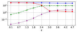
(a) Student Dataset

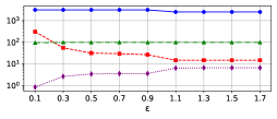
(b) COMPAS Dataset

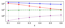
(c) Adult Dataset

Figure 1: Feasibility graph connectivity based on $\epsilon$.

TABLE I: Graph connectivity statistics for each dataset

Metrics	Student		COMPAS		Adult
	$G_{0}$	$G_{1}$	$G_{0}$	$G_{1}$	$G_{0}$	$G_{1}$
Nodes	383	266	1090	1412	16192	32650
Number of Strongly CC	319	229	982	655	7242	8806
Number of Weakly CC	1	2	169	39	987	994
Density (%)	4.21	3.68	0.42	2.47	0.31	0.70

V-A Auditing Fairness

In this set of experiments, we exploit our algorithms to audit fairness. Without loss of generality, we focus on finding counterfactual explanations for the false negative (FN) instances of a classification model (logistic regression) of groups $G_{0}$ and $G_{1}$. We include only instances in $G_{0}$ and $G_{1}$ for which at least one feasible counterfactual exists and use as a cost function, the $L_{2}$ vector distance.

V-A1 Burden

Let us first study the subgroups of groups $G_{0}$ and $G_{1}$ as formed by the WCCs of $G_{U}$. Figure 6 depicts the distribution of factual and candidate counterfactual instances across the WCCs (i.e., subgroups) of each group. The number of WCCs per group is a lower bound for the minimum number $k_{0}$ of counterfactuals required for the full coverage of the group. Further, the ratio of factual and counterfactuals in each WCC provides an indication of the difficulty of providing counterfactuals for each subgroup. For example, in both Compas and Adult, some subgroups of $G_{1}$ are hard to cover.

In Table VIII, we report $k_{0}$ and the minimum cost $d_{0}$ for full coverage. In both the Compas and the Adult datasets, $G_{1}$ requires significantly more counterfactuals for full coverage, due to the larger number of WCCs and the difficulty of covering specific WCCs (as indicated in Figure 6). Across all datasets, $G_{0}$ requires less cost for full coverage. This suggests that $G_{0}$ is easier to cover in general as it requires fewer resources in terms of both the number of counterfactuals and the associated cost.

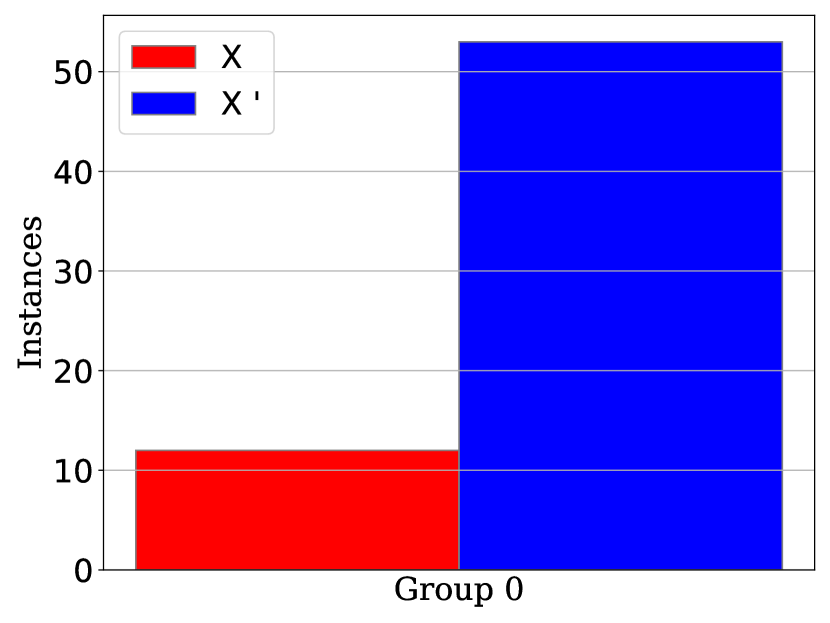
(a) Student $G_{0}$

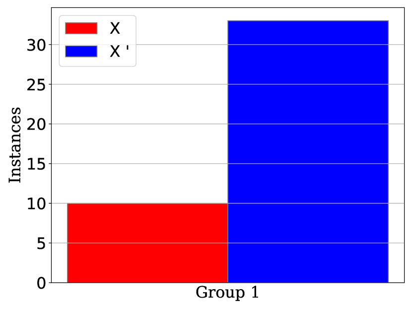
(b) Student $G_{1}$

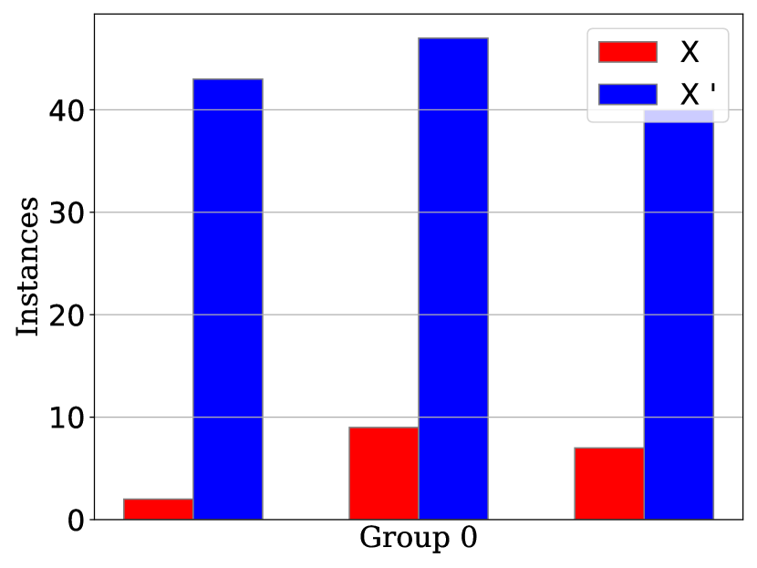
(c) COMPAS $G_{0}$

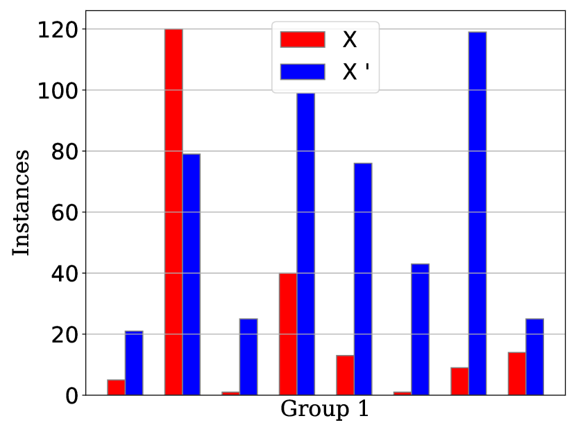
(d) COMPAS $G_{1}$

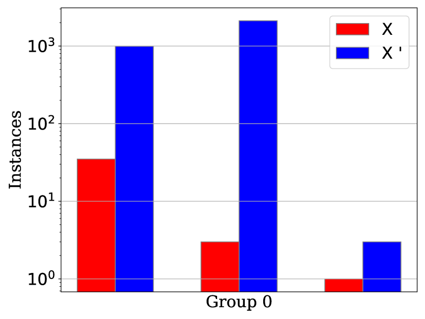
(e) Adult $G_{0}$

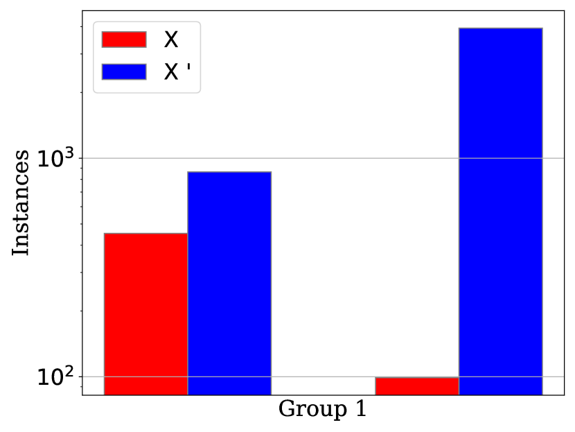
(f) Adult $G_{1}$

Figure 2: Distribution of factuals $X$ and candidate countefactuals $X^{\prime}$ instances for each WCC for each group.

TABLE II: Minimum counterfactuals and cost for coverage.

Datasets	$G_{0}$		$G_{1}$
	$k_{0}$	$d_{0}$	$k_{0}$	$d_{0}$
Student	2	3.71	1	3.98
COMPAS	3	0.57	9	0.61
Adult	5	0.7	12	1.2

Next, we use the AUC-related fairness measures to account for the various trade-offs between the number $k$ of counterfactuals, cost $d$, and coverage $c$. Table IX shows results of the $kAUC$ plots of coverage against cost, Table IV of the $dAUC$ plots of coverage against the number of counterfactuals, and Table V of the $cAUC$ plots of cost against the number of counterfactuals. The AUC scores in Tables IX and IV are normalized using the maximum values for full coverage, while the AUC scores in Table V are normalized using the $cAUC$ of the plot of the minimum cost value in any of the groups against $k$. For $kAUC$ and $dAUC$, the larger the AUC scores, the better, while for $cAUC$ the smaller the AUC scores, the better. More details about normalization and the selection of the $x$-axis values for all AUC plots are in the supplementary material.

The AUC measures provide a deeper analysis of fairness than $k_{0}$ and $d_{0}$. For the Student dataset, Table IX shows that although $G_{1}$ achieves full coverage with $k=1$, $G_{1}$ requires larger costs than $G_{0}$ to achieve full coverage for $k>1$. For large values of $k$, the $AUC$ scores of both groups become similar. Table IV shows that $G_{1}$ can achieve better coverage for lower costs and smaller $k$ values than $G_{0}$. Finally, if we want to optimize for cost efficiency, Table V shows that $G_{1}$ typically requires fewer resources for coverage up to 75%. For the COMPAS dataset, despite the many WCCs of $G_{1}$, Table IX shows that with just $k=1$, $G_{1}$ achieves over 50% coverage and Table IV that $G_{1}$ achieves similar coverage with comparable costs and comparable $AUC$-scores with $G_{0}$. Table V indicates that $G_{0}$ generally requires fewer counterfactuals and incurs lower costs for all coverage levels but for $c=0.75$. For the Adult dataset, $G_{1}$ gets better $kAUC$-scores than $G_{0}$ only for small values of $k$ (Table IX) and requires a large $k$ for coverage even for large costs (Table IV) indicating that there are factuals in $G_{1}$ that are hard to cover. Table V indicates that $G_{1}$ generally requires many counterfactuals and incurs high costs for all coverage levels.

TABLE III: $kAUC$ scores, saturation points $sp$ and maximum possible coverage $max_{cov}$ for various $k$.

$k$	Student						COMPAS						Adult
	$G_{0}$			$G_{1}$			$G_{0}$			$G_{1}$			$G_{0}$			$G_{1}$
	$sp$	$max_{cov}$	$AUC$	$sp$	$max_{cov}$	$AUC$	$sp$	$max_{cov}$	$AUC$	$sp$	$max_{cov}$	$AUC$	$sp$	$max_{cov}$	$AUC$	$sp$	$max_{cov}$	$AUC$
1	4.29	0.82	0.66	4.29	1	0.9	0.43	0.5	0.5	0.73	0.57	0.57	1.14	0.40	0.39	1.44	0.63	0.63
2	3.79	1	0.87	4.29	1	0.92	0.73	0.88	0.88	0.73	0. 77	0.77	0.84	0.60	0.6	1.44	0.83	0.82
3	3.79	1	0.92	4.29	1	0.93	0.73	1	0.99	0.73	0.84	0.84	0.84	0.80	0.8	1.44	0.89	0.88
4	3.79	1	0.95	4.29	1	0.94	0.73	1	1.0	0.73	0.90	0.9	0.84	0.90	0.9	1.44	0.93	0.92
5	3.29	1	0.95	4.29	1	0.94	0.43	1	1.0	0.73	0.95	0.95	0.84	1	1.0	1.44	0.95	0.95
6	3.29	1	0.95	4.29	1	0.94	0.43	1	1.0	0.73	0.97	0.97	0.84	1	1.0	1.44	0.96	0.96
7	3.29	1	0.95	4.29	1	0.94	0.43	1	1.0	0.73	0.99	0.99	0.84	1	1.0	1.44	0.97	0.97
8	3.29	1	0.95	4.29	1	0.94	0.43	1	1.0	0.73	99.5	0.99	0.84	1	1.0	1.44	0.98	0.98
9	3.29	1	0.95	4.29	1	0.94	0.43	1	1.0	0.73	1	1.0	0.84	1	1.0	1.44	0.99	0.98
10	3.29	1	0.95	4.29	1	0.94	0.43	1	1.0	0.73	1	1.0	0.84	1	1.0	1.44	0.99	0.99

TABLE IV: ${dAUC}$ scores, saturation points $sp$ and maximum possible coverage $max_{cov}$ for various $d$.

Student							COMPAS							Adult
$d$	$G_{0}$			$G_{1}$			$d$	$G_{0}$			$G_{1}$			$d$	$G_{0}$			$G_{1}$
	$sp$	$max_{cov}$	$AUC$	$sp$	$max_{cov}$	$AUC$		$sp$	$max_{cov}$	$AUC$	$sp$	$max_{cov}$	$AUC$		$sp$	$max_{cov}$	$AUC$	$sp$	$max_{cov}$	$AUC$
0.1	1	0	0.	1	0	0.0	0.1	2	16.7	0.16	9	0.09	0.07	0.1	1	0.0	0.0	10	0.04	0.03
0.6	1	0	0.0	1	0	0.0	0.4	5	1	0.93	10	0.93	0.82	0.4	6	0.80	0.66	10	0.36	0.25
1.1	1	0	0.0	1	0	0.0	0.7	3	1	0.96	10	0.99	0.91	0.7	5	0.90	0.79	10	0.87	0.74
1.6	1	0	0.0	1	0.11	0.11	1.0	3	1	0.96	9	1	0.91	1.0	5	1	0.89	10	0.98	0.9
2.1	1	0.09	0.09	2	0.22	0.22	1.3	2	1	0.98	4	1	0.97	1.3	5	1	0.89	10	0.99	0.93
2.6	5	0.45	0.37	4	0.55	0.5	1.6	2	1	0.98	4	1	0.97	1.6	5	1	0.89	10	0.99	0.93
3.1	6	0.82	0.67	2	0.89	0.88	1.9	2	1	0.98	4	1	0.97	1.9	5	1	0.89	10	0.99	0.93
3.6	3	1	0.95	1	0.89	0.89	2.2	2	1	0.98	4	1	0.97	2.2	5	1	0.89	10	0.99	0.93
4.1	2	1	0.99	1	1	1.0	2.5	2	1	0.98	4	1	0.97	2.5	5	1	0.89	10	0.99	0.93
4.6	2	1	0.99	1	1	1.0	2.8	2	1	0.98	4	1	0.97	2.8	5	1	0.89	10	0.99	0.93

TABLE V: ${cAUC}$ scores, saturation points ($sp$) and minimum maximum distance $max_{d}$ for various $c$.

$c$	Student						COMPAS						Adult
	$G_{0}$			$G_{1}$			$G_{0}$			$G_{1}$			$G_{0}$			$G_{1}$
	$sp$	$max_{d}$	$AUC$	$sp$	$max_{d}$	$AUC$	$sp$	$max_{d}$	$AUC$	$sp$	$max_{d}$	$AUC$	$sp$	$max_{d}$	$AUC$	$sp$	$max_{d}$	$AUC$
0.25	3	2.42	1.12	3	2.16	1	3	0.11	1	13	0.11	1.06	3	0.19	1	26	0.29	1.64
0.50	4	2.92	1.35	4	2.56	1.18	3	0.14	1.25	13	0.15	1.35	4	0.25	1.32	28	0.38	2.12
0.75	6	3.01	1.44	4	2.62	1.22	6	0.22	1.99	16	0.18	1.80	6	0.39	2.07	27	0.47	2.64
1	6	3.22	1.53	2	3.86	1.76	5	0.36	3.21	12	0.53	4.99	5	0.7	3.67	15	0.93	5.01

V-A2 Attribution

We now look into which attributes in each group contribute the most to the False Negative decisions of the model. To this end, we use $ACF$ which measures how frequently an attribute is changed in a counterfactual compared to the corresponding factual.

In Figure 7, we show attribute descriptions and how frequently their value changes. Only attributes that were modified in more than 50% of the counterfactuals of at least one subgroup are shown. To produce counterfactuals, we solve the coverage-constrained FGCE problem for full coverage, i.e., $c=1$.

In the Student dataset, for $G_{1}$, attributes family educational support and extracurricular activities are frequently altered, indicating the significant role of societal and educational support. Number of school absences, current health status, the age of the student, weekly study time appears in all $G_{1}$ counterfactuals but in only 60% of $G_{0}$ suggestions. Conversely, $G_{0}$ shows a stronger dependence on attributes related to family and personal relationships, such as cohabitational status of parents, quality of family relationships, and in a romantic relationship. This suggests that $G_{0}$ relies more on such personal and familial factors, while $G_{1}$ places a greater emphasis on societal and educational aspects underscoring different weightings in decision-making based on social factors. For the COMPAS dataset, $G_{0}$ shows consistent dependency on age, indicating that it plays a key role in risk assessment. In the Adult dataset, work hours per week and age are the most frequently changed attributes in both groups and nearly always modified for $G_{1}$. Notably, the marital status attribute is only changed in $G_{1}$ counterfactuals, and there is a significant emphasis on relationship status in $G_{1}$ compared to $G_{0}$. This indicates that $G_{1}$ is more sensitive to adjustments in work-related and personal relationship factors.

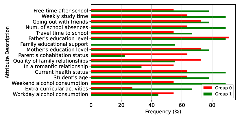
(a) Student Dataset

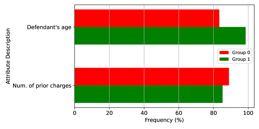
(b) COMPAS Dataset

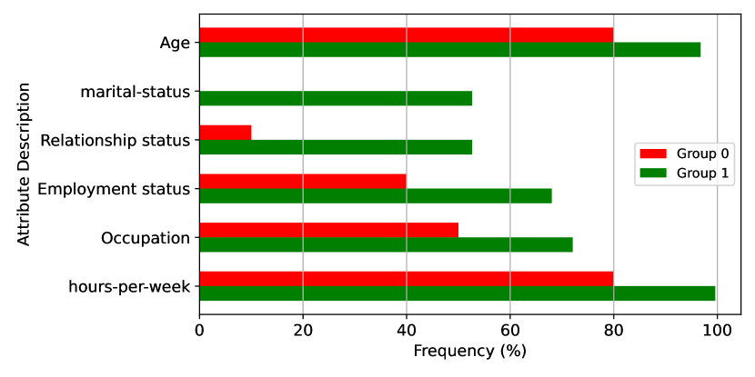
(c) Adult Dataset

Figure 3: Frequency of changes in attributes of CFE suggestions to instances.

V-B Comparison with Baselines

In this set of experiments, we compare the performance of our approach to previous research on generating counterfactuals. We conduct two types of evaluations: (a) against FACE [6], a graph-based method that generates individual counterfactuals, and (b) against two state-of-the-art baselines, AReS [11] and GLOBE-CE [12], which generate group counterfactuals. For this set of experiments, we generate counterfactuals for the whole group $G=G_{0}\cup G_{1}$.

V-B1 Comparison with Individual Counterfactuals

We first compare our approach with FACE [6], an approach that produces counterfactuals for individual factuals using a similar graph-based approach. We apply FACE to locate for each $\mathbf{x}$ $\in$ $X$ the counterfactual $x^{\prime}$ $\in$ $A_{x}$ such that the $cost(\mathbf{x},\mathbf{x}^{\prime})$ is minimized. This can be considered as the optimal counterfactual for $\mathbf{x}$. We use two different cost functions: (a) the $L_{2}$ distance between $\mathbf{x}$ and its counterfactual $\mathbf{x}^{\prime}$ (vector distance) and (b) the length of the shortest path from $\mathbf{x}$ to $\mathbf{x}^{\prime}$ in $G_{U}$, which is defined as the sum of the weights in the shortest path ($W_{ij}$ distance). This is the cost function used in FACE.

We solve the coverage-constrained FGCE problem to generate a set $S$ of counterfactuals for varying values of $k$. For FACE, we generate individual counterfactuals for all factuals covered by the set $S$ returned by FGCE. We then compare the average cost between $\mathbf{x}$ and its optimal counterfactual generated using FACE with the average cost between $\mathbf{x}$ and its counterfactual in set $S$ generated by FGCE. Figure 8 shows the results. Reported distances are normalized by their maximum values.

In the Student dataset, for the $W_{ij}$ distance FACE shows an increase from $k=1$ to $k=2$, stabilizing afterwards. FGCE manages to drop the overall cost when providing more counterfactuals, indicating competitive performance. Considering the vector distances, the FGCE cost remains constant, while FACE shows a slight increase initially. In the COMPAS dataset, both FACE and FGCE show a stepwise decrease in the $W_{ij}$ distance, indicating that FGCE can drop the average cost when possible by providing more counterfactuals. As for the vector distances, FGCE slightly deviates from the ideal counterfactuals. In the Adult dataset, both approaches indicate the need for providing more counterfactuals to reduce their $W_{ij}$ distance, while achieving similar values. Focusing on vector distances, FACE provides consistently low costs, while FGCE requires more counterfactuals to approximate this cost, while still maintaining competitive performance.

Overall, FGCE provides group counterfactuals with cost competitive to the optimal one provided by FACE.

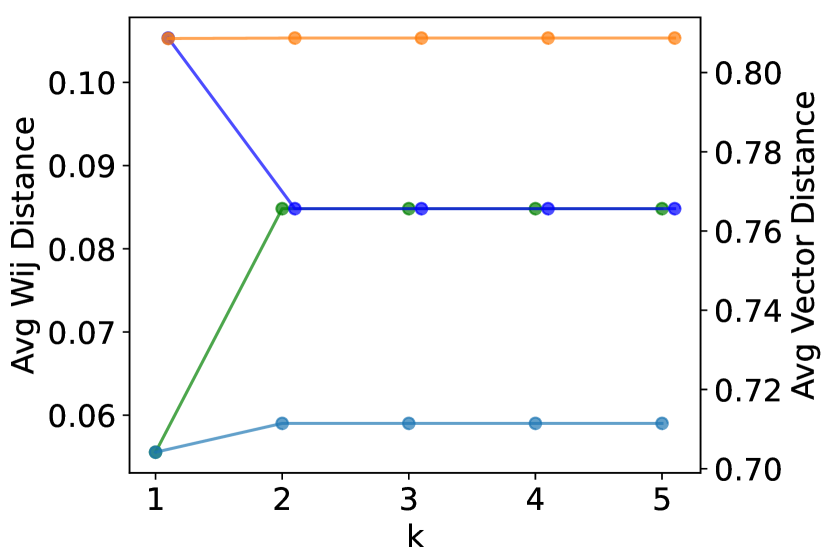
(a) Student Dataset

(b) COMPAS Dataset

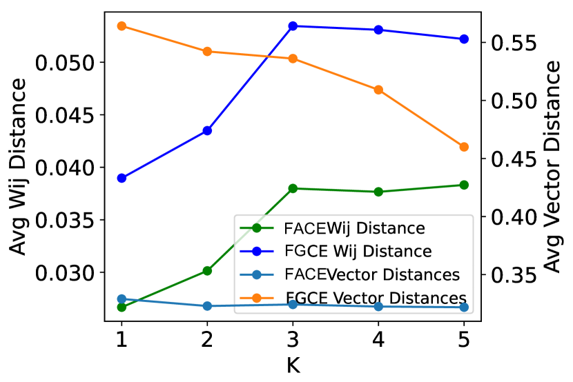
(c) Adult Dataset

Figure 4: FGCE comparison with FACE in terms of average vector distance and average sum of $W_{ij}$ on shortest paths.

V-B2 Comparison with group counterfactuals.

We also compare our approach with two state-of-the-art group counterfactual baselines: AReS [11] that creates rule-based group counterfactuals and GLOBE-CE [12], which employs scaled translation vectors for counterfactual generation. None of them considers feasibility constraints in generating counterfactuals.

For the Student dataset, AReS generates 9 rules ($r$) with max coverage 68%, and for the COMPAS dataset 10 rules with max coverage 85.08%. GLOBE-CE offering scaled translations per factual managed to cover all factuals, i.e. max coverage 100% for both datasets. We do not report results for the Adult dataset, since both competitors have very small coverage.

We assess the feasibility of the generated counterfactuals by first normalizing them, and then integrating them into a feasibility graph $G_{U}$. We quantify coverage as the percentage of feasible paths among factuals and their counterfactuals. We measure cost using the $L_{2}$ distance between the factual and the corresponding counterfactual. To evaluate the effects of varying levels of constraint relaxation on coverage, we generate different $G_{U}$ graphs. Specifically, we remove feasibility constraints (FC) for specific attributes and use two values of $\epsilon$, namely, the default $\epsilon$ value and no $\epsilon$ (i.e., no constraint in distance). The results are summarized in Table VI.

Relaxing FCs improves coverage using the AReS approach across both datasets, whereas achieving coverage with GLOBE-CE necessitates the removal of all constraints. Specifically, in the COMPAS dataset, eliminating the feasibility constraint for the prc (priors_count) attribute, which does not allow decreasing in a counterfactual the count of prior offenses, led to higher coverage rates for AReS. Similarly, in the Student dataset, removing the health attribute appears to increase coverage. With no $\epsilon$, in the COMPAS dataset, we note that the AReS approach maintains 85.08% coverage both with and without constraints, while the GLOBE-CE approach still necessitates the removal of all constraints to achieve coverage.

The FGCE approach achieves a high coverage rate on both datasets while maintaining low costs across all feature constraints. This highlights the strength of our approach in prioritizing feasible and actionable counterfactuals.

TABLE VI: Comparison with group counterfactual baselines.

Student
$\epsilon$	FC	AReS			GLOBE-CE			FGCE
	removed	$r$	Cov.	Cost	$k$	Cov.	Cost	$k$	Cov.	Cost
3	none	9	60	1.1	25	0	0	5	80	2.3
	age	9	60	1.1	25	0	0	5	80	2.3
	health	9	68	1.08	25	0	0	5	80	2.27
	all	9	68	1.08	25	100	0.46	5	80	2.2
-	none	9	60	1.1	25	0	0	5	80	2.3
	age	9	60	1.1	25	0	0	5	80	2.2
	health	9	68	1.08	25	0	0	5	80	2.3
	all	9	68	1.08	25	100	0.46	5	80	2
COMPAS
$\epsilon$	FC	AReS			GLOBE-CE			FGCE
	removed	$r$	Cov.	Cost	$k$	Cov.	Cost	$k$	Cov.	Cost
0.3	none	10	71.9	0.24	228	0	0	9	90	0.24
	age	10	71.9	0.24	228	0	0	9	90	0.21
	prc	10	80	0.25	228	0	0	9	90	0.17
	all	10	85.08	0.26	228	96.49	0.15	9	90	0.17
-	none	10	85.08	0.26	228	0	0	9	90	0.24
	age	10	85.08	0.26	228	0	0	9	90	0.21
	prc	10	85.08	0.26	228	0	0	9	90	0.17
	all	10	85.08	0.26	228	100	0.17	9	90	0.17

VI Related Work

Explanations have become a central focus in recent research [20, 5, 2, 3, 21, 22, 23, 4, 24], particularly as machine learning systems are increasingly employed to inform decisions in critical societal domains such as finance, healthcare, and education.

Counterfactual explanations hold a significant place in the explanations commonly used in the literature. Wachter et al. [25], one of the first works on counterfactual explanations, formulates CEs as an optimization problem that minimizes the distance between the original input and a counterfactual instance while ensuring the desired class prediction. Building upon this, a plethora of methods have been developed [26, 8, 27, 28, 5, 9, 6], each honing in on specific attributes of CEs [5] like validity, actionability, and sparsity and using different techniques. Some employ genetic programming to generate counterfactuals, CERTIFAI  [9], for instance, utilizes an evolutionary algorithm-based approach, evolving potential solutions over multiple generations to ascertain optimal CEs. Others rely on distance-based methods to identify significant changes in the feature space required for class transition, as seen in PreCoF  [28]. Also, methods addressing heterogeneous data utilize optimization techniques based on integer programming  [29], [30]. Furthermore, techniques like FACE [6] ensure that counterfactuals are also feasible and coherent with real-world data distribution, increasing the likelihood of actionable pathways for end-users. Our approach builds upon this concept to generate group feasible counterfactuals, capturing diverse trade-offs of coverage, cost, and interpretability.

While most approaches provide local explanations, focusing on individual instances, there are also group CEs aimed at explaining groups of instances in the input space. AReS [11] extends individual recourse by leveraging two-level recourse sets and formulating an objective function that optimizes for correctness, coverage, cost-effectiveness, and interpretability of the resulting explanations. Another approach in this vein is GLOBE-CE  [12], which defines global CEs as a translation direction multiplied by an input-dependent scalar representing the distance an input must travel to change its prediction. Additionally, CET  [31] leverages decision trees to assign actions to multiple instances opting for transparency and consistency. [32] also generates collective counterfactuals for a group of interest such that the minimizing cost under some linking constraints by solving a convex quadratic linearly constrained mixed integer problem.

None of these methods focuses on finding feasible counterfactuals as we do. While they allow for the exclusion of certain sensitive features, they lack precise control over the direction of increase or decrease permitted for these features. Furthermore, GLOBE-CE generates counterfactuals by selecting randomly features of the dataset and altering their values which can result in counterfactuals that do not align well with the underlying data distribution. In contrast, FGCEs ensure that they both lie in the data manifold and also adhere to the real-world feasibility constraints, thereby enhancing their trust, feasibility, and applicability.

Explanations have recently been used to address concepts of unfairness [4]. Fairness in this context refers to non-discrimination, ensuring that algorithmic decisions are not influenced by irrelevant attributes such as race or gender [33, 34, 35, 36, 37]. There are a few previous approaches that use counterfactuals to understand or measure unfairness [9, 19, 28, 13, 11]. The authors in [9] and [19] generate counterfactuals for individual instances and quantify burden by aggregating the distances between a factual and its counterfactual. PreCof [28] also generates counterfactuals for individual instances and uses the counterfactuals to explain which attributes contribute to unfairness. Instead in this work, we focus on generating group counterfactuals and using them to measure and explain unfairness. By doing so, we aim both at improving interpretability and at capturing the collective behavior of a group as a whole avoiding for example outliers. [9, 19, 28, 13, 11]. AReS [11] does not propose any new fairness measures but just compares the cost of counterfactuals across different racial subgroups. FACTS [13] builds on AReS to generate counterfactuals and posits that a classifier can be deemed fair if it satisfies certain fairness criteria. Our FGCE approach offers enhanced novel fairness measures that allow auditing fairness both at the group and the subgroup level and understanding the trade-offs between the number of counterfactuals, cost, and coverage.

This section presents additional experimental evaluations of the FGCE framework using two extended datasets, German Credit and HELOC. The German Credit dataset classifies individuals as good or bad credit risks based on attributes like credit history and employment. The HELOC dataset contains credit card information, including credit limits and payment history, used to predict credit risk or default likelihood. These experiments aim to demonstrate the adaptability and effectiveness of FGCE to financial contexts, reinforcing the insights gained from the main study. Both datasets involve credit risk assessments, where feasible counterfactuals are crucial for actionable insights.

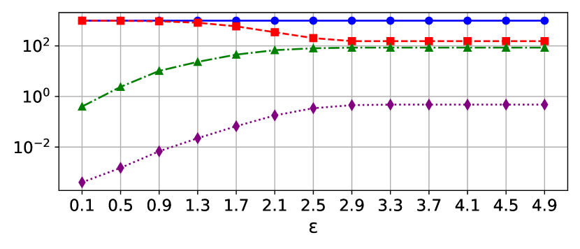
(a) German Credit Dataset

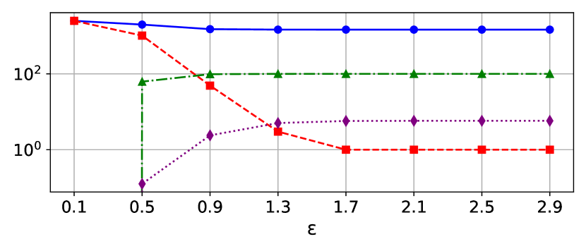
(b) HELOC Dataset

Figure 5: Feasibility graph connectivity based on $\epsilon$.

-A Feasibility Graph

For the German Credit and HELOC datasets, we determine optimal $\epsilon$ values—2.9 and 1.4, respectively—as the minimum thresholds for maximum node connectivity (no singleton nodes), as shown in Figure 5. For the German Credit dataset, we define groups based on gender, with $G_{0}$ representing women and $G_{1}$ representing men. In HELOC, we use the MaxDelqEver attribute to split groups into those with more than 5 delinquencies and those with 5 or fewer. Table VII, presents the structure of the feasibility graph and the components created for each of the groups.

TABLE VII: Graph connectivity statistics for each dataset

Metrics	GermanCredit		HELOC
	$G_{0}$	$G_{1}$	$G_{0}$	$G_{1}$
Nodes	310	690	1090	1412
Number of Strongly CC	310	686	927	539
Number of Weakly CC	59	96	1	1
Density (%)	0.92	0.76	3.68	14.15

-B Auditing Fairness

-B1 Burden

Table VIII shows the minimum counterfactuals for full coverage ($k_{0}$) and minimum maximum cost for full coverage ($d_{0}$). For the German Credit dataset, $G_{0}$ requires fewer counterfactuals and lower costs than $G_{1}$, while the HELOC dataset exhibits the opposite trend. This indicates $G_{0}$ for German Credit and $G_{1}$ for HELOC are easier to cover with fewer resources. Figure 6 depicts the distribution of factual and candidate counterfactual instances across aWCCs for each subgroup. As observed in the main paper, aWCCs with a lower possible counterfactual $X^{\prime}$-to-factual $X$ ratio are harder to cover, as evidenced by $G_{1}$ in 6, which requires more CFEs VIII.

TABLE VIII: Minimum counterfactuals and cost for coverage.

Datasets	$G_{0}$		$G_{1}$
	$k_{0}$	$d_{0}$	$k_{0}$	$d_{0}$
German Credit	1	2.36	5	2.67
HELOC	3	1.65	1	1.54

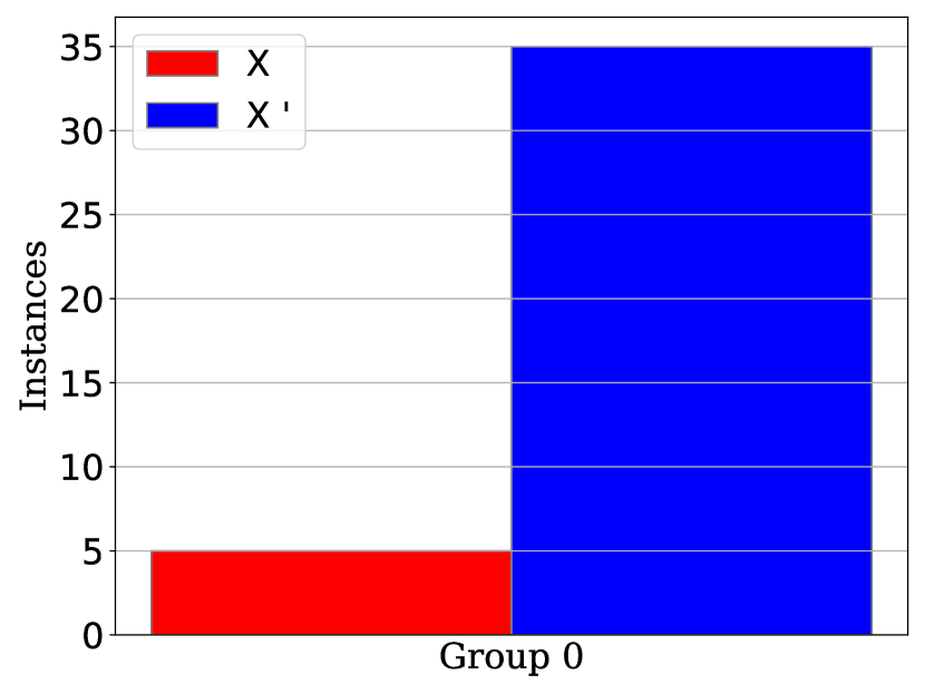
(a) German Credit $G_{0}$

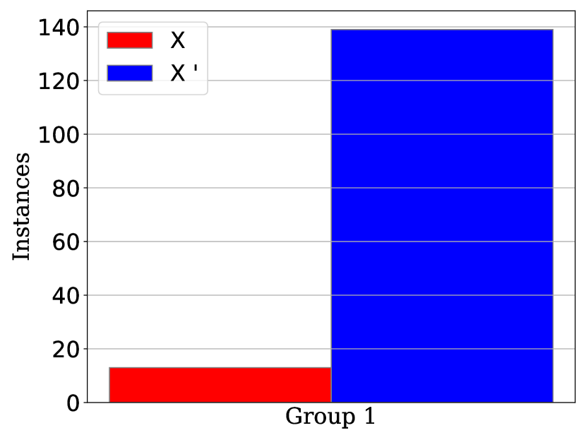
(b) German Credit $G_{1}$

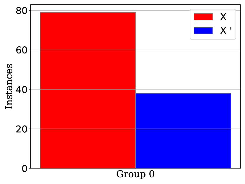
(c) HELOC $G_{0}$

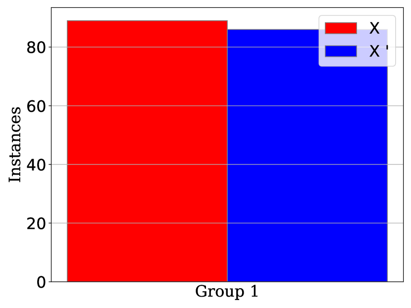
(d) HELOC $G_{1}$

Figure 6: Distribution of factuals $X$ and candidate countefactuals $X^{\prime}$ instances for each WCC for each group.

Next, we use AUC-related fairness metrics to audit the fairness of trade-offs in CFE generation methods. Tables IX and X display the $kAUC$ and $dAUC$ scores, respectively, including their saturation points $sp(k)$ and $sp(d)$, and the coverage percentages at these points. Table XI provides the $cAUC$ scores, saturation points $sp(c)$, and the minimum maximum cost for each coverage level.

In the German Credit dataset, Table IX reveals that $G_{0}$ achieves 100% coverage with the first counterfactual and maintains cost efficiency throughout, indicating a straightforward path to coverage. In contrast, $G_{1}$ reaches full coverage only by the third counterfactual, initially requiring more CFEs and thus facing a more complex path. This complexity is further highlighted by Table X, which shows that while $G_{1}$ starts with lower-cost coverage, $G_{0}$’s efficiency improves over time and eventually requires less overall cost. Table XI reinforces this, demonstrating $G_{0}$’s consistent need for fewer resources to achieve full coverage, suggesting a simpler or less diverse feature interaction compared to $G_{1}$.

The HELOC dataset shows a different pattern. According to Table IX, $G_{1}$ quickly achieves high coverage with fewer counterfactuals, while $G_{0}$ gradually reaches similar performance as more counterfactuals are added, suggesting $G_{1}$’s advantageous position in the feature space and less stringent changes needed to modify outcomes. Conversely, Table X reveals that $G_{1}$ initially provides a small coverage percentage at a low cost but requires many counterfactuals. $G_{1}$ is also the first to achieve full coverage (see also Table VIII), demonstrating better coverage effectiveness with fewer CFEs and lower costs. This implies that $G_{0}$ needs a broader search for feasible counterfactuals, indicating a more complex feature interplay. Lastly, Table XI shows that $G_{1}$ efficiently reaches up to 50% coverage with minimal cost and counterfactuals, while $G_{0}$, though needing more counterfactuals, requires less effort overall to achieve full coverage. The same holds true for $G_{0}$ after the 50% mark, which requires less effort overall based on AUC scores to achieve full coverage but with more counterfactuals.

In summary, AUC-related metrics validate the ability of FGCE to uncover disparities in the effort required for equitable outcomes across different groups. reaffirm the effectiveness of FGCE in auditing fairness in predictive modeling across diverse domains.

TABLE IX: $kAUC$ scores and saturation points

k	German Credit						HELOC
	$G_{0}$			$G_{1}$			$G_{0}$			$G_{1}$
	$sp$	Cov	$AUC$	$sp$	Cov	$AUC$	$sp$	Cov	$AUC$	$sp$	Cov	$AUC$
1	2.67	100.0	0.83	3.07	66.7	0.56	1.65	75.0	0.74	1.65	100.0	0.98
2	2.67	100.0	0.83	3.07	88.9	0.75	1.65	93.75	0.92	1.65	100.0	0.98
3	2.67	100.0	0.83	3.07	100.0	0.85	1.65	100.0	0.99	1.65	100.0	0.98
4	2.67	100.0	0.83	2.67	100.0	0.89	1.65	100.0	0.99	1.65	100.0	0.98
5	2.67	100.0	0.83	2.67	100.0	0.91	1.65	100.0	0.99	1.65	100.0	0.98
6	2.67	100.0	0.83	2.67	100.0	0.91	1.65	100.0	0.99	1.65	100.0	0.98
7	2.67	100.0	0.83	2.67	100.0	0.91	1.65	100.0	0.99	1.65	100.0	0.98
8	2.67	100.0	0.83	2.67	100.0	0.91	1.65	100.0	0.99	1.65	100.0	0.98
9	2.67	100.0	0.83	2.67	100.0	0.91	1.65	100.0	0.99	1.65	100.0	0.98
10	2.67	100.0	0.83	2.67	100.0	0.91	1.65	100.0	0.99	1.65	100.0	0.98

TABLE X: $dAUC$ scores and saturation points

German Credit							HELOC
d	$G_{0}$			$G_{1}$			d	$G_{0}$			$G_{1}$
	$sp$	$Cov$	$AUC$	$sp$	$Cov$	$AUC$		$sp$	$Cov$	$AUC$	$sp$	$Cov$	$AUC$
0.1	1	0.0	0.0	1	0.0	0.0	0.1	1	0.0	0.0	1	0.0	0.0
0.5	1	0.0	0.0	1	0.0	0.0	0.6	1	0.0	0.0	5	15.15	0.14
0.9	1	0.0	0.0	1	0.0	0.0	1.1	4	75.0	0.7	3	71.21	0.71
1.3	1	0.0	0.0	1	0.0	0.0	1.6	2	93.75	0.93	1	100.0	1.0
1.7	3	0.0	0.0	2	22.22	0.22	2.1	3	100.0	0.98	1	100.0	1.0
2.1	3	50.0	0.5	2	44.44	0.44	2.6	3	100.0	0.98	1	100.0	1.0
2.5	3	100.0	1.0	4	100.0	0.93	3.1	3	100.0	0.98	1	100.0	1.0
2.9	3	100.0	1.0	3	100.0	0.97	3.6	3	100.0	0.98	1	100.0	1.0
3.3	3	100.0	1.0	3	100.0	0.97	4.1	3	100.0	0.98	1	100.0	1.0
3.7	3	100.0	1.0	3	100	0.97	4.6	3	100.0	0.98	1	100.0	1.0

TABLE XI: ${cAUC}$ scores and saturation points

c	German Credit						HELOC
	$G_{0}$			$G_{1}$			$G_{0}$			$G_{1}$
	$sp$	$max_{d}$	$AUC$	$sp$	$max_{d}$	$AUC$	$sp$	$max_{d}$	$AUC$	$sp$	$max_{d}$	$AUC$
25	1	2.01	1.15	2	1.75	1.00	3	0.84	1.15	4	0.73	1.00
50	1	2.01	1.15	4	2.05	1.17	6	0.94	1.31	6	0.91	1.24
75	1	2.36	1.35	5	2.35	1.34	4	1.07	1.47	2	1.13	1.51
100	1	2.36	1.35	6	2.57	1.47	3	1.64	1.85	1	1.54	2.04

-B2 Attribution

Next, we assess fairness in counterfactual suggestions using the ACF metric, which tracks how often attributes are altered in counterfactuals versus actual instances. Figure 7 shows the attributes and their alteration percentages, focusing on those changed in over 50% of FGCE recommendations for at least one subgroup. The experiments utilize the parameters $k_{0}$, and $d_{0}$ from VIII for full coverage.

In the German Credit dataset, FGCE attribution analysis shows that group $G_{0}$ relies heavily on financial stability and employment attributes like Duration of present employment, Duration of present residence, Balance or type of the checking account, and Installment rate in percentage of disposable income. In contrast, group $G_{1}$ depends more on Credit duration in months, indicating a focus on credit history for assessing credit risk. This indicates that financial stability and credit history attributes have differential impacts on credit risk assessment, revealing how the model’s focus shifts based on group-specific characteristics.

In the HELOC dataset, FGCE analysis reveals distinct priorities across groups. For $G_{0}$, attributes such as percent of trades with balance, months since most recent delinquency, months since oldest trade open, and percentage of trades with balance are frequently adjusted, highlighting a focus on recent and historical credit behavior. Notably, changes to the Max delinquency ever attribute are suggested only for $G_{0}$. In contrast, $G_{1}$ prioritizes attributes like Number of trades opened in the last 12 months, Net fraction of installment credit to credit limit, and total number of credit trades, indicating a greater emphasis on recent credit activity and overall credit utilization. This differentiation suggests that $G_{0}$ is more concerned with past credit stability, while $G_{1}$ focuses on recent credit activity and credit limits.

In the HELOC dataset, FGCE analysis highlights different priorities across groups. For $G_{0}$, attributes like percent of trades with balance, months since most recent delinquency, months since oldest trade open, and the percentage of trades with balance are frequently adjusted, highlighting a focus on recent and historical credit behavior. Notably, changes to the Max delinquency ever attribute are suggested only for $G_{0}$. In contrast, $G_{1}$ prioritizes attributes like Number of trades opened in the last 12 months, Net fraction of installment credit to credit limit, and total number of credit trades, indicating a greater emphasis on recent credit activity and overall credit utilization. This differentiation suggests that $G_{0}$ is more concerned with past credit stability, while $G_{1}$ focuses on recent credit activity and credit limits.

-C Comparison with Individual Counterfactuals

We compare FGCE with FACE by evaluating the average L2 norm distance and the average sum of shortest path weights $w_{ij}$ between counterfactuals and factual instances where at least one feasible group counterfactual exists and present the results in Figure 8. Both metrics are normalized to assess deviations from FACE’s ideal counterfactuals, with $w_{ij}$ serving as the cost function.

In the German Credit dataset, FGCE demonstrates competitive performance relative to FACE. FGCE effectively maintains $w_{ij}$ costs on par with FACE, while the average vector distance remains comparable to that of FACE. For the HELOC dataset, the $w_{ij}$ costs for both FGCE and FACE decrease at $k=2$ and remain consistent after three counterfactuals, highlighting FGCE’s ability to match FACE in terms of cost efficiency. Vector distance metrics also reflect close alignment between the two approaches.

Overall, FGCE demonstrates competitive performance compared to FACE, effectively capturing group-specific nuances while maintaining similar cost efficiencies and vector distances.

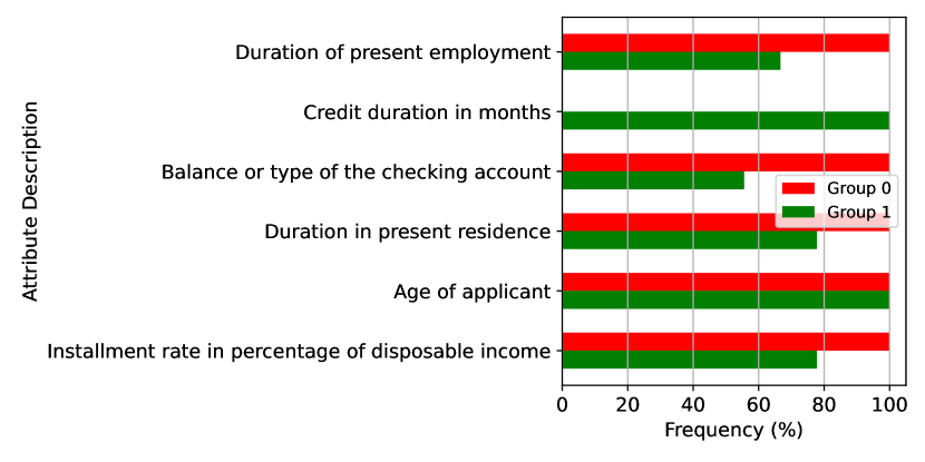
(a) GermanCredit Dataset

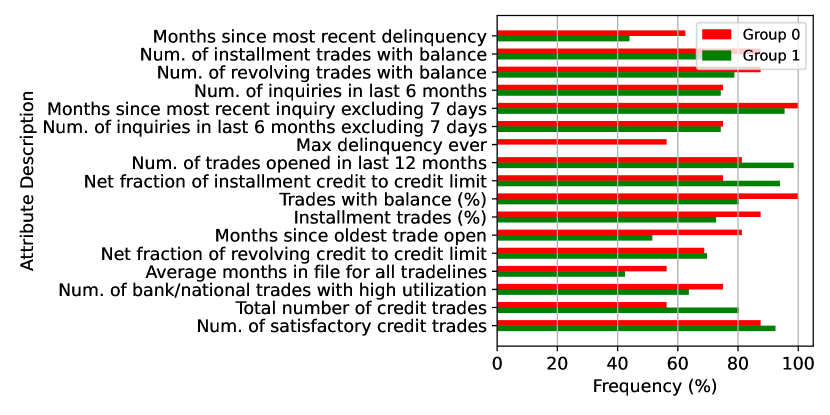
(b) HELOC Dataset

Figure 7: Frequency of changes in attributes of CFE suggestions to instances.

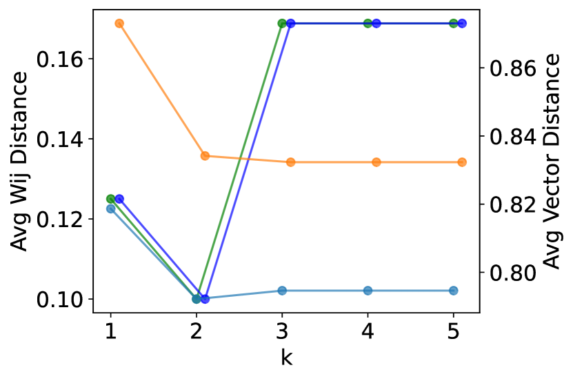
(a) German Credit Dataset

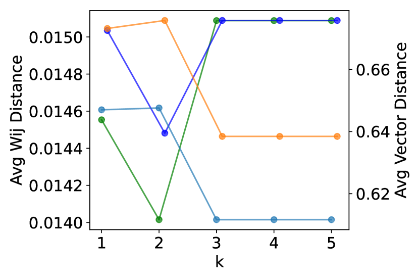
(b) HELOC Dataset

Figure 8: FGCE comparison with FACE in terms of average vector distance and average sum of $w_{ij}$ on shortest paths.

Appendix A Datasets

We employ three datasets; Student , COMPAS , Adult , German Credit and HELOC . The Student dataset includes records of student performance, featuring attributes like study time and family support. The target labels are derived from the final grade (G3), with students categorized as having lower performance if G3 is less than $10$ and high performance if G3 is $10$ or higher. The COMPAS dataset contains instances from the criminal justice system, used to predict the likelihood of recidivism. The Adult dataset comprises records of individuals with attributes related to their income. It is used for classification tasks, specifically to determine if an individual’s annual income exceeds $\$50,000$. The German Credit dataset classifies individuals as either good or bad credit risks based on various attributes such as credit history, account status, and employment. The HELOC dataset, consists of credit card account information, including features such as credit limits, payment history, and credit utilization rates, used for predicting credit risk or the likelihood of default. We treat as continuous, numerical attributes where the values represent measurements or quantities, with many unique values. More details about each attribute description, feasibility constraint, and corresponding datatype of Student, COMPAS, Adult, German Credit, HELOC, can be found in tables XII, XIII, XIV, XV and XVI respectively.

TABLE XII: Attributes, descriptions, feasibility constraints, and data types for the Student dataset. Constraints are denoted as follows: Up arrows ($\uparrow$) indicate attributes where only increases are allowed, down arrows ($\downarrow$) indicate attributes where only decreases are allowed, equals signs ($=$) denote attributes with no allowed changes, and dashes (-) represent attributes with no constraints.

Attribute	Description	Constraints	Dtype
age	Age of student (15 to 22)	$\uparrow$	int64
Medu	Education of mother	$\uparrow$
Fedu	Education of father	$\uparrow$
traveltime	Home to school travel time	-
studytime	Weekly study time	-
failures	Number of past class failures	-
famrel	Quality of family relationships	-
freetime	Free time after school	-
goout	Going out with friends	-
Dalc	Workday alcohol consumption	-
Walc	Weekend alcohol consumption	-
health	Current health status	$\uparrow$
absences	Number of school absences	-
G1	First period grade	-
G2	Second period grade	-
G3	Final grade	-
target	$1\text{ if }G3\geq 10\text{ else }0$	-
school	School of student	-	category
sex	Sex of student	$=$
address	Home address type of student	-
famsize	Family size	$\uparrow$
Pstatus	Cohabitation status of parents	-
Mjob	Job of mother	-
Fjob	Job of father	-
reason	Reason to choose this school	-
guardian	Guardian of student	-
schoolsup	Extra educational support	-
famsup	Family educational support	-
paid	Extra paid classes within the course subject	-
activities	Extra-curricular activities	-
nursery	Attended nursery school	$\uparrow$
higher	Wants to take higher education	-
internet	Internet access at home	-
romantic	with a romantic relationship	-

Appendix B Implementation Details

Density Selection Method Bandwidth selection is a critical aspect of kernel density estimation (KDE) that impacts the smoothness and accuracy of the resulting density estimate. To address this, we offer two methods for bandwidth selection. The first method is based on Scott’s rule [38], a heuristic that balances bias and variance in density estimation. It calculates the bandwidth parameter using the sample size and standard deviation of the data, providing a simple yet effective way to determine bandwidth. Alternatively, for a more refined optimization, we calculate the bandwidth using grid search and cross-validation techniques.

TABLE XIII: Attributes, descriptions, feasibility constraints, and data types for the COMPAS dataset. Constraints are denoted as follows: Up arrows ($\uparrow$) indicate attributes where only increases are allowed, down arrows ($\downarrow$) indicate attributes where only decreases are allowed, equals signs ($=$) denote attributes with no allowed changes, and dashes (-) represent attributes with no constraints.

Attribute	Description	Constraints	Dtype
age	Age of defendant	$\uparrow$	int64
juv_fel_count	Juvenile felony count	$\downarrow$
juv_misd_count	Juvenile misdemeanor count	$\downarrow$
juv_other_count	Juvenile other offenses count	$\downarrow$
priors_count	Prior offenses count	$\downarrow$
sex	Sex of defendant	=	category
c_charge_degree	Charge degree of original crime	$\downarrow$
race	Race of defendant	-
two_year_recid	Whether the defendant is rearrested within 2 years	-

TABLE XIV: Attributes, descriptions, feasibility constraints, and data types for the Adult dataset. Constraints are denoted as follows: Up arrows ($\uparrow$) indicate attributes where only increases are allowed, down arrows ($\downarrow$) indicate attributes where only decreases are allowed, equals signs ($=$) denote attributes with no allowed changes, and dashes (-) represent attributes with no constraints.

Attribute	Description	Constraints	Dtype
age	Age of an individual	$\uparrow$	int64
workclass	Employment status of individual	-
education	Highest level of education attained	$\uparrow$
educational-num	Number of years of education	$\uparrow$
marital-status	Marital status	-
occupation	Occupation of individual	-
relationship	Relationship to the head of household	-
capital-gain	Capital gains in the past year	-
capital-loss	Capital losses in the past year	-
hours-per-week	Hours worked per week	-
sex	Sex of individual	$=$	category
race	Race of individual	$=$

TABLE XV: Attributes, descriptions, feasibility constraints, and data types for the German Credit dataset. Constraints are denoted as follows: Up arrows ($\uparrow$) indicate attributes where only increases are allowed, down arrows ($\downarrow$) indicate attributes where only decreases are allowed, equals signs ($=$) denote attributes with no allowed changes, and dashes (-) represent attributes with no constraints.

Attribute	Description	Constraints	Dtype
Credit-Amount	Amount of credit required	$\downarrow$	Continuous
Month-Duration	Duration of the credit in months	$\downarrow$	int64
Instalment-Rate	Installment rate as a percentage of disposable income	$\downarrow$
Residence	Present residence duration in years	-
Age	Age of the individual	$\uparrow$
Existing-Credits	Number of existing credits at this bank	-
Num-People	Number of people liable to provide maintenance for	-
Existing-Account-Status	Balance or type of the checking account	$\uparrow$	category
Credit-History	Past credit behaviour of individual	*
Purpose	Purpose of the credit (e.g., furniture, education)	-
Savings-Account	Status of savings account/bonds	$\uparrow$
Present-Employment	Duration of present employment	$\uparrow$
Sex	Sex of the applicant	$=$
Marital-Status	Marital status of the applicant	$=$
Guarantors	Presence of guarantors	$\uparrow$
Property	Property ownership	$\downarrow$
Installment	Other installment plans	$\downarrow$
Housing	Housing status (e.g., rent, own, for free)	$\uparrow$
Job	Job type (e.g., unemployed, management)	$\uparrow$
Telephone	Registered telephone under the customers name	$\uparrow$
Foreign-Worker	Whether the applicant is a foreign worker	$=$

TABLE XVI: Attributes, descriptions, feasibility constraints, and data types for the HELOC dataset. Constraints are denoted as follows: Up arrows ($\uparrow$) indicate attributes where only increases are allowed, down arrows ($\downarrow$) indicate attributes where only decreases are allowed, equals signs ($=$) denote attributes with no allowed changes, and dashes (-) represent attributes with no constraints.

Attribute	Description	Constraints	Dtype
AverageMInFile	Average months in file for all trade lines	-	Continuous
NetFraction Install Burden	Net fraction of installment credit to credit limit	$\downarrow$
NetFraction Revolving Burden	Net fraction of revolving credit to credit limit	-
MSinceMostRecent Trade Open	Months since the most recent trade line was opened	-
PercentInstallTrades	Percentage of installment trades	-
PercentTrades WBalance	Percentage of trades with balance	-
NumTotalTrades	Total number of trade lines	-
MSinceMostRecent Delq	Months since the most recent delinquency	$\downarrow$
NumSatisfactoryTrades	Number of satisfactory trade lines	$\uparrow$
PercentTradesNever Delq	Percentage of trades with no delinquency	$\uparrow$
ExternalRisk Estimate	Risk estimate provided by an external source	$\downarrow$
ExternalRisk Estimate	Risk estimate provided by an external source	$\downarrow$	int64
MSinceOldest TradeOpen	Months since the oldest trade was opened	-
NumTrades60Ever2 DerogPubRec	Number of trades that have experienced 60+ days past due or worse	$\downarrow$
NumTrades90Ever2DerogPubRec	Number of trades that have experienced 90+ days past due or worse	$\downarrow$
MaxDelq2Public RecLast12M	Maximum delinquency reported in the last 12 months	$\downarrow$
MaxDelqEver	Maximum delinquency reported ever	$\downarrow$
NumTradesOpenin Last12M	Number of trades opened in the last 12 months	-
MSinceMostRecent Inqexcl7days	Months since most recent inquiry, excluding the last 7 days	-
NumInqLast6M	Number of inquiries in the last 6 months	-
NumInqLast6Mexcl7days	Number of inquiries in the last 6 months, excluding the last 7 days	-
NumRevolvingTrades WBalance	Number of revolving trades with balance	-
NumInstallTrades WBalance	Number of installment trades with balance	-
NumBank2NatlTrades WHigh Utilization	Number of bank/national trades with a high utilization ratio	-
RiskPerformance	Target variable indicating borrower’s risk performance	-	category

MIP algorithm. We implement the MIP approach using the Pulp library [39], with COIN-OR Branch and Cut (CBC) solver which executes the branch-and-cut algorithm. Baselines comparison. To compare our approach with baselines, for FACE and GLOBE-CE, we utilize their respective code repositories available on GitHub. For AReS, we employ the code provided by GLOBE-CE as no dedicated repository exists.

Preprocess Our preprocessing pipeline is consistent across datasets including the treatment of categorical and numerical data, which often poses challenges in these tasks. For ordered categorical features, we allow for a user-defined order that is dataset-specific, offering flexibility to accommodate natural sequences where applicable. In contrast, unordered categorical features, such as job occupations, are one-hot encoded to ensure that the difference between any two categories is consistent and maximally distinct, without implying any order or magnitude of change. Binary categorical features are label-encoded. For continuous features, we discretize them into bins using a heuristic algorithm that determines the number of bins based on the logarithm of the number of unique values and the range of those values, ensuring a balance between granularity and practicality. Last, we normalize each feature to the range of $[0,1]$, ensuring an equal contribution of features.

Although some datasets require additional tailored adjustments. From the COMPAS dataset, we exclude the attributes age_cat and c_charge_desc. The age_cat attribute which bins ages into categories was excluded due to its strong correlation coefficient of $0.99$ with age. Similarly, the c_charge_desc attribute was omitted because of its high correlation coefficient of $0.91$ with c_charge_degree, a binary attribute indicating misdemeanor or felony status. Retaining age_cat and c_charge_degree simplifies handling binary attributes. For the GermanCredit dataset, we split the original sex attribute, which contains information about sex and marital status, into two distinct attributes: sex and marital status [40]. To create feasibility constraints, we adjust certain feature values as follows: For the ”Existing-Account-Status” feature we map the value ’A14’ to ’A10’that account status can only improve in the proposed counterfactual instance after encoding. Similarly, for the ”Savings account/bonds” feature we map ’A65’ to ’A60’ to impose constraints that allow only increases in savings in the proposed counterfactual instance. Additionally, for the ”Credit-History” feature we set the constraint that if the instance value is A34 or A33, it can change to A32, A31, or A30, ensuring an improved credit history while permitting all other possible transitions. For the HELOC dataset, we drop any row with at least one negative value in their columns.

Appendix C Hyper-parameters

Models. Our experiments employ the Logistic Regression model from scikit-learn, utilizing its default settings for classification tasks. The datasets are divided into training and test sets with a 70% to 30% ratio, respectively. For reproducibility, we use a random seed value of 482 in the ‘train_test_split‘ function from scikit-learn. FGCE is applied exclusively to the test set.

Upper Bound Cost Limit In our experiments, the upper bound for the cost limit is defined by the square root of the effective number of features post-preprocessing. Each set of binary indicators of one-hotted features is counted as a single feature, and the target variable is excluded. Since we normalize all features to the range $[0,1]$, the upper bound represents the maximum Euclidean distance between two hypothetical instances: one where all features are at their minimum (zero) and another where all are at their maximum (one), thus setting a practical yet expansive limit for cost evaluations between any two instances within the dataset.

Optimal $k$AUC and $d$AUC Scores The optimal $k$AUC and $d$AUC scores are computed by evaluating the AUC of the values along the x-axis (number of counterfactuals $k$ for $k$AUC, or distances $d$ for $d$AUC) while maintaining the coverage at its maximum. These optimal scores provide a baseline for normalization, ensuring that the $k$AUC and $d$AUC scores reflect the best achievable performance across all $k$ or $d$ values, respectively.

Optimal $c$AUC score The $cAUC$ score is calculated by evaluating $cAUC$ for common $k$ values across groups. The optimal $cAUC$ score is determined by identifying the minimum cost among all groups for each shared $k$, and using this minimum cost for all common $k$ values to compute the metric. This approach ensures that the optimal $cAUC$ reflects the lowest effort required across all groups for a given coverage level. The resulting optimal $cAUC$ score is then used to normalize the $cAUC$ scores.

Cost used for $kAUC$ scores computations range from 70% of the minimum required for full coverage to the maximum possible cost per dataset. Tables showing the $dAUC$ scores list score values for 10 cost levels from 0.1 to the maximum possible per dataset with a step defined as $(\text{max possible distance}-0.1)/10$, while counterfactuals ranging from 1 to 10.

References

- [1] A.-H. Karimi, G. Barthe, B. Schölkopf, and I. Valera, “A survey of algorithmic recourse: contrastive explanations and consequential recommendations,” ACM Computing Surveys, vol. 55, no. 5, pp. 1–29, 2022.
- [2] F. Bodria, F. Giannotti, R. Guidotti, F. Naretto, D. Pedreschi, and S. Rinzivillo, “Benchmarking and survey of explanation methods for black box models,” Data Mining and Knowledge Discovery, vol. 37, no. 5, pp. 1719–1778, 2023.
- [3] R. Dwivedi, D. Dave, H. Naik, S. Singhal, R. Omer, P. Patel, B. Qian, Z. Wen, T. Shah, G. Morgan et al., “Explainable ai (xai): Core ideas, techniques, and solutions,” ACM Computing Surveys, vol. 55, no. 9, pp. 1–33, 2023.
- [4] C. Fragkathoulas, V. Papanikou, D. P. Karidi, and E. Pitoura, “On explaining unfairness: An overview,” in 2024 IEEE 40th International Conference on Data Engineering Workshops (ICDEW), 2024, pp. 226–236.
- [5] S. Verma, V. Boonsanong, M. Hoang, K. Hines, J. Dickerson, and C. Shah, “Counterfactual explanations and algorithmic recourses for machine learning: A review,” ACM Comput. Surv., jul 2024, just Accepted. [Online]. Available: https://doi.org/10.1145/3677119
- [6] R. Poyiadzi, K. Sokol, R. Santos-Rodriguez, T. De Bie, and P. Flach, “Face: feasible and actionable counterfactual explanations,” in Proceedings of the AAAI/ACM Conference on AI, Ethics, and Society, 2020, pp. 344–350.
- [7] M. T. Ribeiro, S. Singh, and C. Guestrin, “” why should i trust you?” explaining the predictions of any classifier,” in Proceedings of the 22nd ACM SIGKDD international conference on knowledge discovery and data mining, 2016, pp. 1135–1144.
- [8] R. K. Mothilal, A. Sharma, and C. Tan, “Explaining machine learning classifiers through diverse counterfactual explanations,” in Proceedings of the 2020 conference on fairness, accountability, and transparency, 2020, pp. 607–617.
- [9] S. Sharma, J. Henderson, and J. Ghosh, “Certifai: A common framework to provide explanations and analyse the fairness and robustness of black-box models,” in Proceedings of the AAAI/ACM Conference on AI, Ethics, and Society, ser. AIES ’20. New York, NY, USA: Association for Computing Machinery, 2020, p. 166–172. [Online]. Available: https://doi.org/10.1145/3375627.3375812
- [10] L. E. Bynum, J. R. Loftus, and J. Stoyanovich, “Counterfactuals for the future,” in Proceedings of the AAAI Conference on Artificial Intelligence, vol. 37, no. 12, 2023, pp. 14 144–14 152.
- [11] K. Rawal and H. Lakkaraju, “Beyond individualized recourse: Interpretable and interactive summaries of actionable recourses,” Advances in Neural Information Processing Systems, vol. 33, pp. 12 187–12 198, 2020.
- [12] D. Ley, S. Mishra, and D. Magazzeni, “Globe-ce: A translation-based approach for global counterfactual explanations,” arXiv preprint arXiv:2305.17021, 2023.
- [13] L. Kavouras, K. Tsopelas, G. Giannopoulos, D. Sacharidis, E. Psaroudaki, N. Theologitis, D. Rontogiannis, D. Fotakis, and I. Emiris, “Fairness aware counterfactuals for subgroups,” Advances in Neural Information Processing Systems, vol. 36, 2024.
- [14] M. Rosenblatt, “Remarks on Some Nonparametric Estimates of a Density Function,” The Annals of Mathematical Statistics, vol. 27, no. 3, pp. 832 – 837, 1956. [Online]. Available: https://doi.org/10.1214/aoms/1177728190
- [15] D. S. Hochba, “Approximation algorithms for np-hard problems,” ACM Sigact News, vol. 28, no. 2, pp. 40–52, 1997.
- [16] B. C. Tansel, R. L. Francis, and T. J. Lowe, “Location on networks: A survey. part i: The p-center and p-median problems,” Management Science, pp. 482–497, 1983.
- [17] M. Daskin, “Network and discrete location: models, algorithms and applications,” Journal of the Operational Research Society, vol. 48, no. 7, pp. 763–764, 1997.
- [18] S. Verma and J. Rubin, “Fairness definitions explained,” in FairWare@ICSE. ACM, 2018, pp. 1–7.
- [19] A. Kuratomi, E. Pitoura, P. Papapetrou, T. Lindgren, and P. Tsaparas, “Measuring the burden of (un) fairness using counterfactuals,” in Joint European Conference on Machine Learning and Knowledge Discovery in Databases. Springer, 2022, pp. 402–417.
- [20] C. Molnar, Interpretable machine learning. Lulu.com, 2020.
- [21] A. B. Arrieta, N. Díaz-Rodríguez, J. Del Ser, A. Bennetot, S. Tabik, A. Barbado, S. García, S. Gil-López, D. Molina, R. Benjamins et al., “Explainable artificial intelligence (xai): Concepts, taxonomies, opportunities and challenges toward responsible ai,” Information fusion, vol. 58, pp. 82–115, 2020.
- [22] A. Adadi and M. Berrada, “Peeking inside the black-box: a survey on explainable artificial intelligence (xai),” IEEE access, vol. 6, pp. 52 138–52 160, 2018.
- [23] R. Guidotti, “Counterfactual explanations and how to find them: literature review and benchmarking,” Data Mining and Knowledge Discovery, pp. 1–55, 2022.
- [24] M. A. Prado-Romero, B. Prenkaj, G. Stilo, and F. Giannotti, “A survey on graph counterfactual explanations: definitions, methods, evaluation, and research challenges,” ACM Computing Surveys, vol. 56, no. 7, pp. 1–37, 2024.
- [25] S. Wachter, B. Mittelstadt, and C. Russell, “Counterfactual explanations without opening the black box: Automated decisions and the gdpr,” Harv. JL & Tech., vol. 31, p. 841, 2017.
- [26] R. Guidotti, A. Monreale, F. Giannotti, D. Pedreschi, S. Ruggieri, and F. Turini, “Factual and counterfactual explanations for black box decision making,” IEEE Intelligent Systems, vol. 34, no. 6, pp. 14–23, 2019.
- [27] K. Kanamori, T. Takagi, K. Kobayashi, and H. Arimura, “Dace: Distribution-aware counterfactual explanation by mixed-integer linear optimization.” in IJCAI, 2020, pp. 2855–2862.
- [28] S. Goethals, D. Martens, and T. Calders, “Precof: counterfactual explanations for fairness,” Machine Learning, vol. 113, no. 5, pp. 3111–3142, 2024.
- [29] C. Russell, “Efficient search for diverse coherent explanations,” in Proceedings of the conference on fairness, accountability, and transparency, 2019, pp. 20–28.
- [30] B. Ustun, A. Spangher, and Y. Liu, “Actionable recourse in linear classification,” in Proceedings of the conference on fairness, accountability, and transparency, 2019, pp. 10–19.
- [31] K. Kanamori, T. Takagi, K. Kobayashi, and Y. Ike, “Counterfactual explanation trees: Transparent and consistent actionable recourse with decision trees,” Proceedings of Machine Learning Research, vol. 151, pp. 1846–1870, 2022.
- [32] E. Carrizosa, J. Ramírez-Ayerbe, and D. R. Morales, “Generating collective counterfactual explanations in score-based classification via mathematical optimization,” Expert Systems with Applications, vol. 238, p. 121954, 2024.
- [33] E. Pitoura, K. Stefanidis, and G. Koutrika, “Fairness in rankings and recommendations: an overview,” The VLDB Journal, pp. 1–28, 2022.
- [34] N. Mehrabi, F. Morstatter, N. Saxena, K. Lerman, and A. Galstyan, “A survey on bias and fairness in machine learning,” ACM computing surveys (CSUR), vol. 54, no. 6, pp. 1–35, 2021.
- [35] S. A. Friedler, C. Scheidegger, and S. Venkatasubramanian, “The (im) possibility of fairness: Different value systems require different mechanisms for fair decision making,” Communications of the ACM, vol. 64, no. 4, pp. 136–143, 2021.
- [36] S. Caton and C. Haas, “Fairness in machine learning: A survey,” ACM Computing Surveys, vol. 56, no. 7, pp. 1–38, 2024.
- [37] A. Castelnovo, R. Crupi, G. Greco, D. Regoli, I. G. Penco, and A. C. Cosentini, “A clarification of the nuances in the fairness metrics landscape,” Scientific Reports, vol. 12, no. 1, p. 4209, 2022.
- [38] D. W. Scott, Multivariate density estimation: theory, practice, and visualization. John Wiley & Sons, 2015.
- [39] S. Mitchell, M. OSullivan, and I. Dunning, “Pulp: a linear programming toolkit for python,” The University of Auckland, Auckland, New Zealand, vol. 65, 2011.
- [40] T. Le Quy, A. Roy, V. Iosifidis, W. Zhang, and E. Ntoutsi, “A survey on datasets for fairness-aware machine learning,” Wiley Interdisciplinary Reviews: Data Mining and Knowledge Discovery, vol. 12, no. 3, p. e1452, 2022.