Analytic evaluation of the three-loop three-point form factor of $\operatorname{tr}\phi^{3}$ in $\mathcal{N}=4$ sYM

Abstract

We compute analytically the three-loop correlation function of the local operator $\text{tr}\,\phi^{3}$ inserted into three on-shell states, in maximally supersymmetric Yang-Mills theory. The result is expressed in terms of Chen iterated integrals. We also present our result using generalised polylogarithms, and evaluate them numerically, finding agreement with a previous numerical result in the literature. We observe that the result depends on fewer kinematic singularities compared to individual Feynman integrals. Furthermore, upon choosing a suitable definition of the finite part, we find that the latter satisfies powerful symbol adjacency relations similar to those previously observed for the $\text{tr}\,\phi^{2}$ case.

1 Introduction

Form factors, i.e. the correlation function of (the Fourier transform of) a local operator, inserted into on-shell states are interesting objects in quantum field theory. For example, the simplest form factors of a current inserted into two on-shell states can be used to study the anomalous magnetic moment of the leptons Aoyama:2017uqe; Laporta:2019fmy, and they are useful in the study of infrared divergences (see Collins:1989bt for a review). In particular they have been used to obtain state-of-the-art results for the cusp and collinear anomalous dimension Henn:2016wlm; Boels:2017skl; Lee:2019zop; Henn:2019rmi; Henn:2019swt; vonManteuffel:2020vjv; Lee:2021lkc.

In this paper we focus on form factors in maximally supersymmetric Yang-Mills theory (sYM). The results obtained in such a toy theory can serve as a blueprint for corresponding QCD form factors. In particular, it is interesting to see which simplifications occur when assembling the full form factor from individual Feynman integrals. Moreover, the methods employed here for dealing with the necessary Feynman integrals in dimensional regularisation are general, and will be useful for future QCD studies. Indeed, the same Feynman integrals are relevant for studying processes involving the coupling of a Higgs boson to three gluons, in an effective field theory setup with a large top quark mass.

In sYM, many studies focused on scattering amplitudes on the one hand, and on correlation functions on the other hand, and on relations between them, in particular in the context of a duality with Wilson loops Alday:2007hr; Drummond:2007aua; Brandhuber:2007yx; Drummond:2007cf; Alday:2010zy; Eden:2010zz. From this viewpoint, form factors represent an interesting ‘hybrid’ object of one off-shell composite operator, inserted into a set of on-shell states.

There is a rich literature on form factors in sYM, going back to reference vanNeerven:1985ja, whose authors studied the stress-tensor multiplet inserted into two on-shell states. Many of the techniques known from scattering amplitudes, and properties known from them carry over to form factors. For example, on-shell techniques may be used to obtain integrands to high loop orders (cf. Yang:2019vag for a review). The integrand of the two-point form factor mentioned above is known up to the five-loop level Yang:2016ear; Boels:2012ew, and has been integrated up to four loops Gehrmann:2011xn; Huber:2019fxe; Lee:2021lkc. Although the integrands of the two-point form factors are fascinating, and their integrated expressions contain important information on anomalous dimensions, their kinematic dependence is fixed entirely by dimensional analysis, as those two-point form factors depend only on a single scale, $s=(p_{1}+p_{2})^{2}$. Therefore, it is interesting to study multi-point form factors (i.e., a local operator inserted into $n>2$ on-shell states). Already for $n=3$, one then obtains interesting two-variable functions. The same functions are also relevant for processes such as Higgs plus jet production, or vector boson for jet production.

The simplest three-point form factors to consider is the case of the stress-tensor multiplet, represented e.g. by the component $\text{tr}\,\phi^{2}$, inserted into three on-shell states, as in Brandhuber:2012vm. (For related studies of other local operators, and for more external states, cf. Brandhuber:2014ica; Brandhuber:2016fni; Brandhuber:2018xzk; Brandhuber:2018kqb; Ahmed:2019nkj). The two-loop result of Brandhuber:2012vm is already quite interesting. As was remarked in that reference, the result is closely related to a formula for six-particle MHV amplitudes; moreover, the function space, conveniently described by the symbol method Goncharov:2010jf, is rather simple: the symbol is built from six symbol letters only. In the QCD literature, that function space is known under the name of two-dimensional harmonic polylogarithms Gehrmann:2001jv.

Recently, interest in these form factors was reignited due to a number of novel structural observations. Firstly, it was noticed independently in references Chicherin:2020umh and Dixon:2020bbt that the types of two-loop integrals have a hidden structure: their symbol expressions are not arbitrary words in the six alphabet letters, but rather satisfy certain adjacency relations. Those six adjacency relations forbid specific subsequent appearances of letters, thereby reducing the admissible function space. The authors of reference Chicherin:2020umh interpreted these relations in the context of the surprising fact that the six alphabet letters are associated to a B2/C2 cluster algebra. Secondly, in the reference Dixon:2021tdw it was found that there is a relationship between that form factor, and six-particle MHV amplitudes in sYM (see also Dixon:2022xqh). The precise relationship involves a kinematic map as well as an antipodal duality. (An earlier observed two-loop relationship Brandhuber:2014ica between the two quantities does not appear to generalise.)

An interesting and impressive application of these observations is to turn them into bootstrap assumptions for what structures to expect at higher loop orders. Doing so has made it possible to bootstrap the stress-energy three-point form factor to five Dixon:2020bbt, and all the way up to eight loops Dixon:2022rse. Those bootstrap results are validated by their agreement with recent independent results about the near-collinear limit obtained via integrability Sever:2020jjx; Sever:2021nsq; Sever:2021xga; Basso:2023bwv. The above results are all the more remarkable, as individual Feynman diagrams do not satisfy some of the assumptions about the symbol alphabet (and adjacency relations) already at three loops Henn:2023vbd.

The above results strongly motivate us to investigate the $\text{tr}\,\phi^{3}$ three-point form factor. Its two-loop expression was computed in Brandhuber:2014ica. At three loops, the integrand of this form factor was constructed in Lin:2021kht; Lin:2021qol, where it was also evaluated numerically at one phase-space point. (Four-loop integrands for the form factor of the stress-tensor are available as well Lin:2021lqo.) However, to date, no analytic results for the three-loop form factor have been reported in the literature, due to the lack of knowledge of the three-loop non-planar Feynman integrals appearing in it.

In this paper we evaluate the necessary Feynman integrals analytically using the method of canonical differential equations Henn:2013pwa, extending previous results for planar Feynman integrals DiVita:2014pza; Canko:2020gqp; Canko:2021xmn; Henn:2023vbd, and use them to evaluate the form factor. These missing integrals are a subset of the non-planar three-loop Feynman integrals relevant to Higgs boson decays to three partons. That set of integrals has been recently computed in Gehrmann:2024tds.

We begin by checking the expected singular structure of the three-point $\text{tr}\,\phi^{3}$ form factor up to three loops, by following the iterative infrared structure of amplitudes in $\mathcal{N}=4$ sYM, from the Bern-Dixon-Smirnov (BDS) normalisation Bern:2005iz; Henn:2011by. When constructing the BDS remainder for $\text{tr}\,\phi^{3}$ at three loops, we observe that certain analytical properties (adjacency relations), which are manifest in the two-loop remainder, are no longer satisfied. The existence of such normalisation was recently reported in Dixon:2024talk. This normalisation is inspired by the bootstrapped remainder functions of the three-point $\text{tr}\,\phi^{2}$, constructed up to eight loops Dixon:2020bbt; Dixon:2022rse. In our work, by constructing the form factor from first principles and ensuring all adjacency relations are satisfied, we identify a normalisation that enforces these conditions that we refer to as the BDS-like normalisation.

This paper is organised as follows. In Sec. 2, we give an overview on the three-point form factors $\text{tr}\,\phi^{2}$ and $\text{tr}\,\phi^{3}$, by discussing their kinematic configuration, the construction of the finite remainders through the BDS and BDS-like normalisation, and summarise analytic properties of these form factors. Then, in Sec. 3, we review the known finite remainders for the form factor $\text{tr}\,\phi^{3}$ up to two loops. For the purpose of calculating the three-loop finite remainders, we extend these results to higher orders in the dimensional regulator $\epsilon$ (up to transcendental weight six functions). In Sec. 4, we present our main result: the three-point $\text{tr}\,\phi^{3}$ form factor to three loops. We detail the analytic calculation of the three-loop finite remainder, verify it against the only available numerical evaluation, and provide benchmark numerical results along with two- and three-dimensional plots. We also discuss the analytic properties of this form factor, with a particular focus on our chosen normalisation for the BDS-like normalisation. Lastly, in Sec. LABEL:sec:discussion, we draw our conclusions and discuss directions and open questions.

In the arXiv submission of this paper, we include ancillary files containing detailed information on the computations presented in the following sections. We provide the decomposition of the three-loop form factor $\text{tr}\,\phi^{3}$ in terms of masters integrals (3L_phi3_UT.m), together with their integral family definition (3L_families.m) and the basis of relevant master integrals (with up to nine propagators) (3L_MIs.m), and the analytic expressions of the BDS and BDS-like finite remainder functions in terms of generalised polylogarithms (phi3_GPL.m) and Chen iterated integrals (phi3_CII.m) up to three loops.

2 Three-point form factors in ${\cal N}=4$ super Yang-Mills

In this section, we recall the main features of the form factors that describe the interaction of three on-shell states $\Phi$ and a gauge invariant operator $\mathcal{O}$. This form factor is defined as the Fourier transformations of the matrix elements of the operator taken between the vacuum and three on-shell particle states,

$$\mathcal{F}_{\mathcal{O}}\left(p_{1},p_{2},p_{3};q\right)=\int d^{D}x\,e^{-\imath q\cdot x}\langle\Phi_{1}\Phi_{2}\Phi_{3}|\mathcal{O}\left(x\right)|0\rangle\,.$$ (1)

External states are on-shell $p_{i}^{2}=0$ and the operator carries an off-shell momentum $q^{2}\neq 0$. We can define the kinematic invariants,

$$s_{12} =(p_{1}+p_{2})^{2}\,,$$ (2)

$$s_{13} =(p_{1}+p_{3})^{2}\,,$$ (3)

$$s_{23} =(p_{2}+p_{3})^{2}\,.$$ (4)

Due to momentum conservation, $q=p_{1}+p_{2}+p_{3}$, only three of them are independent,

$$q^{2} =s_{12}+s_{23}+s_{13}\,.$$ (5)

We work in the Euclidean region,

$$q^{2}<0\,,\qquad s_{12}<0\,,\qquad s_{13}<0\,,\qquad s_{23}<0\,,$$ (6)

and consider the dimensionless ratios,

$$u=\frac{-s_{12}}{-q^{2}}\,, v=\frac{-s_{13}}{-q^{2}}\,, w=\frac{-s_{23}}{-q^{2}}\,,$$ (7)

satisfying the condition $u+v+w=1$. The Euclidean region in these variables corresponds to, $0<u<1$ and $0<v<1-u$ (or $0<v<1$ and $0<u<1-v$ ), where $w$ has been expressed in terms of $u$ and $v$.

We focus on the half-BPS form factors $\mathcal{O}(x)=\mathcal{O}_{k}=\text{tr}(\phi^{k})$. For their calculation, we consider the perturbative expansion in the ’t Hooft coupling for the gauge group $\mathsf{SU(N_{c})}$,

$$g^{2}=\frac{g_{\text{YM}}^{2}N_{c}}{e^{\epsilon\gamma_{E}}(4\pi)^{2-\epsilon}}\,,$$ (8)

with $\gamma_{E}$ the Euler-Mascheroni constant,

$$\mathcal{F}_{\mathcal{O}_{k}} =\mathcal{F}_{\mathcal{O}_{k}}^{\left(0\right)}\,c_{k}\,\mathcal{G}_{k}\,\delta^{(4)}(q-p_{1}-p_{2}-p_{3})\,.$$ (9)

Here $c_{k}$ accounts for the colour structures and $\mathcal{F}_{\mathcal{O}_{k}}^{\left(0\right)}$ for the tree-level form factors. For $k=2$ and $k=3$, we have,

$$\mathcal{F}_{\mathcal{O}_{2}}^{\left(0\right)}=\frac{\left\langle 12\right\rangle^{2}}{\left\langle 12\right\rangle\left\langle 23\right\rangle\left\langle 31\right\rangle}\,, c_{2}=\tilde{f}^{a_{1}a_{2}a_{3}}\,,$$ (10)

$$\mathcal{F}_{\mathcal{O}_{3}}^{\left(0\right)}=1\,, c_{3}=\tilde{d}^{a_{1}a_{2}a_{3}}\,,$$ (11)

and the perturbative expansion of $\mathcal{G}_{k}$,

$$\mathcal{G}_{k}=\left(1+\sum_{\ell=1}^{\infty}g^{2\ell}\,\mathcal{G}_{k}^{(\ell)}\right)\,.$$ (12)

Notice that it is expected that under exchange (or permutations) of the external momenta this form factor remains unchanged. This can also be argued from the indistinguishability of the three external on-shell states.

These operators are part of a half-BPS multiplet of operators and corresponds to a generalisation of the chiral part of the stress-tensor multiplet Eden:2011ku; Eden:2011yp. The evaluation of this form factor has been studied up to two loops for all $k$, by explicitly computing it from first principles Brandhuber:2012vm; Brandhuber:2014ica. Very recently, the evaluation of $\mathcal{O}_{2}$ and $\mathcal{O}_{3}$ has been performed in a fully numerical framework Lin:2021kht; Lin:2021qol, by employing unitarity-based methods and colour-kinematics duality. In parallel, bootstrapping techniques have allowed for the extension of the calculation of $\mathcal{O}_{2}$ up to eight loops Dixon:2020bbt; Dixon:2022rse.

Since form factors and, in general, multi-loop scattering amplitudes display infrared (IR) singularities that originate from soft and collinear configurations of the loop momenta, it is possible to predict their IR structure by systematically accounting for universal operators acting on the same amplitudes at lower loop orders Catani:1998bh; Becher:2009qa. Thus, one defines a finite remainder function,

$$\mathcal{G}_{k}=\mathcal{G}_{k}^{\text{BDS}}\exp(\mathcal{R}_{k})\,,$$ (13)

with $\mathcal{G}_{k}^{\text{BDS}}$ corresponding to the exponentiated one-loop factor,

$$\mathcal{G}_{k}^{\text{BDS}} =\exp\left[\sum_{\ell=1}^{\infty}g^{2\ell}\left(f^{\left(\ell\right)}\left(\epsilon\right)\mathcal{G}_{k}^{\left(1\right)}\left(\ell\epsilon\right)+C^{\left(\ell\right)}\right)\right]\,.$$ (14)

This leads to consider the perturbative expansion of the finite remainder, starting at two loops,

$$\mathcal{R}_{k} =\sum_{\ell=2}^{\infty}g^{2\ell}\,\mathcal{R}^{(\ell)}_{k}\,.$$ (15)

Explicitly, by combining Eqs. (12) and (13), the two- and three-loop finite remainder functions admit the form,

$$\mathcal{R}^{\left(2\right)}_{k} =\mathcal{G}_{k}^{\left(2\right)}\left(\epsilon\right)-\frac{1}{2}\left(\mathcal{G}_{k}^{\left(1\right)}\left(\epsilon\right)\right)^{2}-f^{\left(2\right)}\left(\epsilon\right)\mathcal{G}_{k}^{\left(1\right)}\left(2\epsilon\right)-C^{\left(2\right)}+\mathcal{O}\left(\epsilon\right)\,,$$ (16)

$$\mathcal{R}^{\left(3\right)}_{k} =\mathcal{G}_{k}^{\left(3\right)}\left(\epsilon\right)+\frac{1}{3}\left(\mathcal{G}_{k}^{\left(1\right)}\left(\epsilon\right)\right)^{3}-\mathcal{G}_{k}^{\left(2\right)}\left(\epsilon\right)\mathcal{G}_{k}^{\left(1\right)}\left(\epsilon\right)-f^{\left(3\right)}\left(\epsilon\right)\mathcal{G}_{k}^{\left(1\right)}\left(3\epsilon\right)-C^{\left(3\right)}+\mathcal{O}\left(\epsilon\right)\,,$$ (17)

with,

$$f^{\left(1\right)}\left(\epsilon\right) =1+\mathcal{O}(\epsilon)\,,$$

$$C^{(1)} =0\,,$$ (18a)

$$f^{\left(2\right)}\left(\epsilon\right) =-2\zeta_{2}-2\zeta_{3}\epsilon-2\zeta_{4}\epsilon^{2}+\mathcal{O}(\epsilon^{3})\,,$$ (18b)

$$C^{\left(2\right)} =4\zeta_{4}\,,$$ (18c)

$$f^{\left(3\right)}\left(\epsilon\right) =4\left[\frac{11}{2}\zeta_{4}+\left(6\zeta_{5}+5\zeta_{2}\zeta_{3}\right)\epsilon+\left(\frac{1909}{48}\zeta_{6}+31\zeta_{3}^{2}\right)\epsilon^{2}\right]+\mathcal{O}(\epsilon^{3})\,,$$ (18d)

$$C^{(3)} =16\zeta_{3}^{2}-\frac{181}{3}\zeta_{6}\,.$$ (18e)

Alternatively to the BDS normalisation (13), one can consider a different normalisation (or define a BDS-like normalised amplitude), to expose further properties of the finite remainder. This normalisation was extremely useful to expose constraints from the Steinmann relations in the calculation of six- and seven-point amplitudes Caron-Huot:2016owq; Dixon:2016nkn, and was employed in the computation of the leading colour contribution of the form factor $\text{tr}\,\phi^{2}$ through eight loops Dixon:2020bbt; Dixon:2022rse. This normalisation can schematically be expressed as,

$$\mathcal{G}_{k}=\mathcal{G}_{k}^{\text{BDS-like}}\times\mathcal{E}_{k}\,,$$ (19)

with,

$$\mathcal{G}^{\text{BDS-like}} =\mathcal{G}^{\text{BDS}}\exp\left(-\frac{1}{4}\Gamma_{\text{cusp}}\,\mathcal{E}_{k}^{\left(1\right)}\right)\,,$$ (20)

the cusp anomalous dimension Beisert:2006ez,

$$\Gamma_{\text{cusp}}=4g^{2}-8\zeta_{2}g^{4}+88\zeta_{4}g^{6}-4\left(219\zeta_{6}+8\zeta_{3}^{2}\right)g^{8}+\mathcal{O}(g^{10})\,.$$ (21)

$\mathcal{E}$ admitting a perturbative expansion in the coupling constant,

$$\mathcal{E}_{k}=\sum_{L=1}^{\infty}g^{2L}\,\mathcal{E}^{(L)}_{k}\,.$$ (22)

This amounts to the relation between $\mathcal{E}$ and $\mathcal{R}$,

$$\mathcal{E}_{k}=\exp\left[\frac{1}{4}\Gamma_{\text{cusp}}\mathcal{E}^{(1)}_{k}+\mathcal{R}_{k}\right]\,.$$ (23)

In the bootstrapping calculation of the form factor $\text{tr}\,\phi^{2}$, it has been observed that the normalised one-loop function $\mathcal{E}^{(1)}$ becomes Caron-Huot:2016owq; Dixon:2016nkn; Caron-Huot:2019bsq; Dixon:2020bbt; Dixon:2022rse,

$$\mathcal{E}_{2}^{\left(1\right)} =2\left[\text{Li}_{2}\left(1-\frac{1}{u}\right)+\text{Li}_{2}\left(1-\frac{1}{v}\right)+\text{Li}_{2}\left(1-\frac{1}{w}\right)\right]\,.$$ (24)

For $\text{tr}\,\phi^{3}$, the existence of such normalisation that satisfies similar analytic properties to the form factor $\text{tr}\,\phi^{2}$ has been reported in Dixon:2024talk. In this work, by explicitly calculating the three-loop contribution to $\mathcal{G}_{3}$ and ensuring that the analytic properties manifest in $\mathcal{G}_{2}$ are also present in $\mathcal{G}_{3}$, we find that the following normalisation choice in Eq. (20) leads to the desired properties,

$$\mathcal{E}^{\left(1\right)}_{3} =-\frac{1}{2}\left[\log^{2}\left(\frac{u}{v}\right)+\log^{2}\left(\frac{v}{w}\right)+\log^{2}\left(\frac{w}{u}\right)\right]-3\zeta_{2}\,.$$ (25)

We shall postpone the discussion on the construction of $\mathcal{E}_{3}^{(1)}$ to Sec. 4.4, where we explore in detail the analytic properties we aim to manifest in $\mathcal{E}_{3}$, by taking advantage of the three-loop contribution to $\mathcal{G}_{3}$.

3 $\text{tr}\,\phi^{3}$ three-point form factor to two loops

In this section, we revisit the known results for the form factor $\text{tr}\,\phi^{3}$ up to two loops, with a focus on the necessary components for the calculation of the three-loop finite remainder (see Eq. (17)). The strategies employed in these calculations are reused in our new three-loop results presented in Sec. 4.

The analytic expressions of this form factor up to two loops can be cast in the sum of $d\log$ integrals up to an overall normalisation factor,

$$\mathcal{G}_{3}^{\left(1\right)} =\sum_{i=1}^{3}\mathcal{I}\left(\parbox{56.9055pt}{\includegraphics[scale={0.4}]{1l_utbw.pdf}}\,s_{i+1\,i+2}\right)\,,$$ (26a)

$$\mathcal{G}_{3}^{\left(2\right)} =\sum_{i=1}^{3}\frac{1}{3}\mathcal{I}\left(\parbox{56.9055pt}{\includegraphics[scale={0.4}]{2l_ut13bw.pdf}}\,s_{i\,i+1}s_{i+1\,i+2}\right)+\frac{1}{3}\mathcal{I}\left(\parbox{56.9055pt}{\includegraphics[scale={0.4}]{2l_ut13bbw.pdf}}\,s_{i\,i+1}s_{i+1\,i+2}\right)$$

$$-\mathcal{I}\left(\parbox{56.9055pt}{\includegraphics[scale={0.4}]{2l_ut3bw.pdf}}\,s_{i\,i+2}\right)+2\mathcal{I}\left(\parbox{56.9055pt}{\includegraphics[scale={0.4}]{2l_ut7bw.pdf}}\,(q^{2}-s_{i+1\,i+2})\right)$$

$$-3\mathcal{I}\left(\parbox{56.9055pt}{\includegraphics[scale={0.4}]{2l_ut10bw.pdf}}\,s_{i+1\,i+2}\right)+\mathcal{I}\left(\parbox{56.9055pt}{\includegraphics[scale={0.4}]{2l_ut14bw.pdf}}\,s_{i+1\,i+2}^{2}\right)\,,$$ (26b)

where $\mathcal{I}\left(\mathcal{N}\right)$ corresponds to the Feynman integral constructed from the propagators present in the loop topology with numerator $\mathcal{N}$ and $s_{i\,j}\equiv(p_{i}+p_{j})^{2}$. Notice that (26b) exactly corresponds to (Brandhuber:2014ica, Eq. (3.24)) once integration-by-parts identities (IBPs) Chetyrkin:1981qh; Laporta:2000dsw are employed to express their integrand in terms of our choice of master integrals, which by construction admit a $d\log$ representation Henn:2020lye; Henn:2021aco.

The analytic expression of the form factor at one loop is known at all orders in the dimensional regulator $\epsilon$,

$$\mathcal{G}_{3}^{(1)}=S_{\epsilon}\frac{1}{\epsilon^{2}}\sum_{i=1}^{3}\left(-s_{i\,i+1}\right)^{-\epsilon}\,,$$ (27)

with $S_{\epsilon}=e^{\epsilon\gamma_{E}}\Gamma(1+\epsilon)\Gamma^{2}(1-\epsilon)/\Gamma(1-2\epsilon)$. The analogous two-loop expression can be expressed in terms of generalised polylogarithms, whose set of planar integrals were computed in Gehrmann:2000zt up to transcendental weight four.

Let us now draw our attention to the two-loop contribution to $\mathcal{G}_{3}$. The analytic expression for the finite remainder $\mathcal{R}_{3}^{(2)}$ has been reported in Brandhuber:2014ica, whose remainder is purely expressed in terms of classical polylogarithms, and their arguments depend on the dimensionless ratios (7). Likewise, the normalised two-loop remainder $\mathcal{E}_{3}^{(2)}$ is obtained after expanding (23) up to order $g^{4}$,

$$\mathcal{E}^{(2)} =\mathcal{R}^{(2)}+\frac{1}{2}\left(\mathcal{E}^{(1)}\right)^{2}-2\zeta_{2}\,\mathcal{E}^{(1)}\,.$$ (28)

This amounts to,

$$\mathcal{E}_{3}^{\left(2\right)}= \frac{3}{2}\left[\text{Li}_{4}\left(-\frac{uv}{w}\right)+\text{Li}_{4}\left(-\frac{uw}{v}\right)+\text{Li}_{4}\left(-\frac{vw}{u}\right)\right]-3\left[\text{Li}_{4}(u)+\text{Li}_{4}(v)+\text{Li}_{4}(w)\right]$$

$$-\frac{3}{2}\log(w)\left[\text{Li}_{3}\left(-\frac{u}{v}\right)+\text{Li}_{3}\left(-\frac{v}{u}\right)\right]$$

$$-\frac{3}{2}\log(v)\left[\text{Li}_{3}\left(-\frac{u}{w}\right)+\text{Li}_{3}\left(-\frac{w}{u}\right)\right]$$

$$-\frac{3}{2}\log(u)\left[\text{Li}_{3}\left(-\frac{v}{w}\right)+\text{Li}_{3}\left(-\frac{w}{v}\right)\right]$$

$$+\frac{9}{16}\left(\log^{4}(u)+\log^{4}(v)+\log^{4}(w)\right)$$

$$-\left(\log^{3}(u)\log(vw)+\log^{3}(v)\log(wu)+\log^{3}(w)\log(uv)\right)$$

$$+26\left(\log^{2}(u)\log^{2}(v)+\log^{2}(v)\log^{2}(w)+\log^{2}(w)\log^{2}(u)\right)$$

$$-\frac{1}{4}\left(\log^{2}(u)\log(v)\log(w)+\log^{2}(v)\log(w)\log(u)+\log^{2}(w)\log(u)\log(v)\right)$$

$$+\frac{1}{4}\zeta_{2}\Big{[}25\left(\log^{2}(u)+\log^{2}(v)+\log^{2}(w)\right)$$

$$\qquad-22\left(\log(u)\log(v)+\log(u)\log(w)+\log(v)\log(w)\right)\Big{]}$$

$$+\zeta_{3}\log(uvw)+\frac{199}{8}\zeta_{4}\,.$$ (29)

The symbol expansion of the two-loop remainder $\mathcal{E}_{3}^{(2)}$ becomes,

$$\mathcal{S}\left(\mathcal{E}_{3}^{\left(2\right)}\right)= -\frac{1}{2}u\otimes\frac{u}{(1-u)^{3}}\otimes\frac{v}{w}\otimes\frac{v}{w}-u\otimes v\otimes\frac{u}{w}\otimes_{S}\frac{v}{w}+6u\otimes\frac{u}{v}\otimes\frac{u}{v}\otimes\frac{u}{v}$$

$$+\text{perms}\left(u,v,w\right)\,,$$ (30)

in terms of the dimensionless ratios (7), $\text{perms}(u,v,w)$ accounting for all six permutations of $\{u,v,w\}$, and the symmetrised tensor product, $x\otimes_{S}y=x\otimes y+y\otimes x$.

Figure 1: Integral families present in the evaluation of the one- and two-loop form factor $\text{tr}\left(\phi^{3}\right)$.

As a prelude for the construction of the three-loop finite remainder, let us remark that one needs to consider one- and two-loop contributions to $\text{tr}\,\phi^{3}$, according to Eq. (16). While the one-loop result is known to all orders in $\epsilon$ (see Eq. (27)), we are required to extend the two-loop contribution to transcendental weight six (or $\epsilon^{2}$ in the dimensional regulator). The integral families involved are depicted in Fig. 1. These integrals are known from references Gehrmann:2023etk; Badger:2023xtl. In the present work, we independently evaluate these integrals so as to have the results in the same format as the three-loop integrals. We compute them in the Euclidean region (6), following the procedure outlined in Henn:2023vbd, and express them in terms of generalised polylogarithms. Due to the structure of the form factor, permutations of the external momenta must be considered when calculating these integrals (see (26b)). The differential equations satisfied by these integrals are solved for the same variables, $u$ and $v$ of Eq. (7), allowing for straightforward analytic cancellations.

As cross-check of our analytic calculation, we recompute the two-loop finite remainders $\mathcal{R}_{3}^{(2)}$ and $\mathcal{E}_{3}^{(2)}$, and obtain the three-loop IR structure of $\mathcal{G}_{3}^{(3)}$ from lower loop orders, according to (17). We handle the products of lower loop contributions to $\mathcal{G}_{3}$ (i.e., $(\mathcal{G}^{(1)}_{3})^{n}$ and $\mathcal{G}^{(1)}_{3}\mathcal{G}^{(2)}_{3}$ with $n=2,3$) with the aid of PolyLogTools Duhr:2019tlz, which are expressed in terms of a minimal set of generalised polylogarithms (GPLs) Parker:2015cia. We construct this basis up to transcendental weight six functions, by systematically enumerating Lyndon words on the sets $\{0,1\}$ and $\{0,1,-v,1-v\}$.

With all one- and two-loop contributions at hand, we now turn our attention to the complete three-loop calculation of the finite remainder, which is the focus of the following section.

4 $\text{tr}\,\phi^{3}$ three-point form factor to three loops

In this section, we analytically calculate the three-loop form factor $\langle\text{tr}(\phi^{3})\phi(p_{1})\phi(p_{2})\phi(p_{3})\rangle$. We have considered the integrands of Lin:2021kht; Lin:2021qol as our starting point.

The three-loop integrand can pictorially cast as,

$$\mathcal{G}_{3}^{\left(3\right)} =\mathcal{I}\left(\parbox{71.13188pt}{ \includegraphics[scale={0.4}]{figs/graphicsN2labelpbw.pdf} }\,\mathcal{N}_{2}\right)\,+\mathcal{I}\left(\parbox{71.13188pt}{ \includegraphics[scale={0.4}]{figs/graphicsN3labelpbw.pdf} }\,\mathcal{N}_{3}\right)\,+\mathcal{I}\left(\parbox{71.13188pt}{ \includegraphics[scale={0.4}]{figs/graphicsN4labelpbw.pdf} }\,\mathcal{N}_{4}\right)\,$$

$$+\mathcal{I}\left(\parbox{71.13188pt}{ \includegraphics[scale={0.4}]{figs/graphicsN5labelpbw.pdf} }\,\mathcal{N}_{5}\right)\,+\mathcal{I}\left(\parbox{71.13188pt}{ \includegraphics[scale={0.4}]{figs/graphicsN9labelpbw.pdf} }\,\mathcal{N}_{9}\right)\,+\mathcal{I}\left(\parbox{71.13188pt}{ \includegraphics[scale={0.4}]{figs/graphicsN11labelpbw.pdf} }\,\mathcal{N}_{11}\right)\,$$

$$+\mathcal{I}\left(\parbox{71.13188pt}{ \includegraphics[scale={0.4}]{figs/graphicsN21labelpbw.pdf} }\,\mathcal{N}_{21}\right)\,+\mathcal{I}\left(\parbox{71.13188pt}{ \includegraphics[scale={0.4}]{figs/graphicsN22labelpbw.pdf} }\,\mathcal{N}_{22}\right)+\text{perms}(p_{1},p_{2},p_{3})\,,$$ (31)

with “$\text{perms}\left(p_{1},p_{2},p_{3}\right)$” accounting for all six permutations of the external massless momenta, and $\mathcal{N}$ are numerators containing dependence on external and internal momenta. Here, $\mathcal{N}_{i}$ exactly matches the i-th diagram of (Lin:2021qol, Fig. 12).

To analytically evaluate the three-loop contribution to $\text{tr}\,\phi^{3}$, $\mathcal{G}^{(3)}_{3}$, we employ established techniques for calculating multi-loop scattering amplitudes. We summarise our methodology in Sec. 4.1. We proceed to analytically construct $\mathcal{G}^{(3)}_{3}$, and the remainder functions $\mathcal{R}^{(3)}_{3}$ and $\mathcal{E}^{(3)}_{3}$, in terms of two-dimensional generalised polylogarithms, in Sec. 4.2. We then compare our results with the only available numerical evaluation reported in Lin:2021kht; Lin:2021qol and present representative two- and three-dimensional plots of the finite remainders, in Sec. 4.3. In the subsequent Sec. 4.4, we proceed to analyse their analytic structure to elucidate further properties of the $\text{tr}\,\phi^{3}$ three-point form factor at three loops. We examine the functional expressions in detail, particularly highlighting the differences between $\mathcal{R}^{(3)}_{3}$ and $\mathcal{E}^{(3)}_{3}$, and providing a support to the BDS-like normalisation, presented in Sec. 3.

4.1 Result in terms of master integrals

(a) Integral family A

(b) Integral family $E_{1}$

(c) Integral family $E_{2}$

(d) Integral family $F_{1}^{*}$

(e) Integral family $I_{2}^{*}$

Figure 2: Integral families present in the evaluation of the three-loop form factor $\text{tr}\left(\phi^{3}\right)$. For integral families $F_{1}^{*}$ and $I_{2}^{*}$, we only consider all possible subtopologies with nine internal propagators.

		Ordering of $\{p_{1},p_{2},p_{3}\}$
Family	123	132	213	231	312	321	Total
A	78	73	46	71	44	40	352
$E_{1}$	12	10	11	10	11	10	64
$E_{2}$	23	20	18	19	18	14	112
$F_{1}^{*}$	32	26	28	22	23	19	150
$I_{2}^{*}$	2	0	0	0	0	0	2

Table 1: Decomposition of the three-loop form factor $\text{tr}\,\phi^{3}$ in terms of master integrals according to the ordering of external momenta in integral family.

In order to calculate $\mathcal{R}_{3}^{\left(3\right)}$ and $\mathcal{E}_{3}^{\left(3\right)}$, we first evaluate $\mathcal{G}_{3}^{\left(3\right)}$. We employ the standard approach for computing multi-loop scattering amplitudes. We start mapping the integrals appearing in (31) onto the families shown in Fig. 2, with the aid of Reduze Studerus:2009ye; vonManteuffel:2012np. Then, we apply IBP identities to reduce the integrals to a minimal set of master integrals, chosen to be in canonical form Henn:2013pwa. For this purpose, we employ LiteRed Lee:2012cn to generate IBPs and sector symmetries between integral families, and FiniteFlow Peraro:2019svx to solve the linear system of equations over finite fields Klappert:2019emp; Peraro:2016wsq; vonManteuffel:2014ixa. We find that $\mathcal{G}_{3}^{\left(3\right)}$ is expressed as a linear combination of 680 master integrals, which, by construction, are uniform transcendental degree integrals, and whose coefficients are rational numbers. Thus, displaying that $\mathcal{G}_{3}^{\left(3\right)}$ manifests uniform transcendental degree at all orders in $\epsilon$, in the very same way as lower loop contributions (see Eqs. (26)).

In Table 1, we summarise the number of master integrals that appear in the decomposition of $\mathcal{G}^{(3)}_{3}$, according to the order of the external momenta. An additional explanation of this table is in order. As previously mentioned, we have implemented sector mappings between all integrals using LiteRed. This is carried out while preserving the order of the integral families listed in the first column ({A, $E_{1}$, $E_{2}$, $F_{1}^{*}$, $I_{2}^{*}$}) and the first row ({{123}, {132}, {213}, {231}, {312}, {321}}). Specifically, we map families from the rightmost part of the lists onto those in the leftmost part of the same list. For example, consider the integrand with numerator $\mathcal{N}_{9}$ in Eq. (31) (pictorially corresponding to a nine-propagator subsector of the integral family $F_{1}^{*}$), with the external momenta ordered as {231} (i.e. $\{p_{2},p_{3},p_{1}\}$). From this table, it can be seen that subsectors of $F_{1}^{*}$ (with less than nine propagators) have been mapped onto A, $E_{1}$, and $E_{2}$, as well as onto subsectors that only appear in $F_{1}^{*}$ but for different orderings of external momenta, such as {{123}, {132}, {213}}.

4.2 Discussion of the Feynman integrals

With the decomposition of $\mathcal{G}^{(3)}_{3}$ in terms of master integrals at our disposal, we proceed to analytically evaluate the three-loop Feynman integrals involved in this decomposition (see Fig. 2 and Table 1). The three-loop planar integrals (A, $E_{1}$, and $E_{2}$) have already been computed, showing dependence solely on the letters of the alphabet $\vec{\alpha}_{u}$ (38), and are expressed in terms of two-dimensional generalised polylogarithms (cf. DiVita:2014pza; Canko:2020gqp; Canko:2021xmn; Henn:2023vbd). For the remaining integral families, $F_{1}^{*}$ and $I_{2}^{*}$, we focus on the relevant nine-propagator subsector to obtain integrals with uniform transcendental degree and solve their canonical differential equations for this specific sector. A brief comment on the analytic structure of these integrals is in order. While the required subsector of $I_{2}^{*}$ depends solely on the letters of the alphabet $\alpha_{u}$, the relevant subsector of $F_{1}^{*}$ exhibits dependence on additional letters that start appearing at transcendental weight four. Remarkably, upon substituting the analytic expressions for the master integrals, we observe pairwise cancellations of these additional letters, resulting in $\mathcal{G}^{(3)}_{3}$ being expressed only in terms of $\vec{\alpha}_{u}$. In this paper, we focus on the analytic calculation of $\mathcal{G}^{(3)}_{3}$. Let us remark that the complete results for all master integrals shown in Fig. 2, including those integral families contributing to the three-loop scattering amplitudes relevant to Higgs boson decays to three partons, have been recently computed in Gehrmann:2024tds. For an overview of the framework employed in these calculations, we refer the reader to this thorough reference.

4.3 Result for remainder function and checks

We obtain the finite remainders $\mathcal{R}^{(3)}$ and $\mathcal{E}^{(3)}$ from the contributions of $\mathcal{G}_{3}$ up to three loops, according to Eqs. (17) and (23). Similar to the calculation of the two-loop remainder discussed in Sec. 3, we observe the analytic cancellation of all infrared poles up to transcendental weight five. Thus, we express the finite remainders $\mathcal{R}^{(3)}$ and $\mathcal{E}^{(3)}$ in terms of 85 generalised polylogarithms.

$(s_{12},s_{13},s_{23})$	$\epsilon^{-6}$	$\epsilon^{-5}$	$\epsilon^{-4}$	$\epsilon^{-3}$	$\epsilon^{-2}$	$\epsilon^{-1}$	$\epsilon^{0}$
$(-2,-2,-2)$	$\underline{-4.5}$	$\underline{9.35748}69$	$\underline{-6.0280}719$	$\underline{31.503}061$	$\underline{19.56}3942$	$\underline{123.5}7978$	$\underline{216}.98716$
$(-1,-1,-2)$	$-4.5$	$3.1191623$	$1.8994028$	$30.694938$	$62.552040$	$189.20903$	$438.75261$
$(-1,-2,-2)$	$-4.5$	$6.2383246$	$-1.3436550$	$30.266438$	$40.558842$	$149.76105$	$314.26322$
$(-1,-2,-3)$	$-4.5$	$8.0629176$	$-4.9111558$	$32.562137$	$28.204878$	$142.41474$	$262.28451$

Table 2: Numerical evaluation of $\mathcal{G}_{3}^{(3)}$ appearing in Eq. (31). The underlined digits show the agreement with the results reported in (Lin:2021kht, Table 1).

$(u,v,w)$	$\mathcal{R}^{(3)}$	$\mathcal{E}^{(3)}$
$(1/3,1/3,1/3)$	198.6040626686176	53.53642538022867
$(1/4,1/4,1/2)$	205.3528021206956	36.90938731982311
$(1/5,2/5,2/5)$	201.0771454928365	30.62853770987929
$(1/2,1/3,1/6)$	205.5332888628428	10.44614318690575

Table 3: Numerical evaluation of the three-loop finite reminders $\mathcal{R}^{(3)}$ and $\mathcal{E}^{(3)}$.

In Tables 2 and 3, we present numerical evaluations of $\mathcal{G}^{(3)}_{3}$, and the finite remainders $\mathcal{R}^{(3)}$ and $\mathcal{E}^{(3)}$ in reference points inside the region (6). We find full agreement with the numerical evaluation of the phase-space point $(s_{12},s_{13},s_{23})=(-2,-2,-2)$ reported in Lin:2021kht; Lin:2021qol.

Let us remark that in Brandhuber:2014ica, with the explicit calculation of the two-loop finite remainder $\mathcal{R}^{(2)}$, it was observed that this remainder diverges at the boundaries of the region (6), specifically at $u=0,v=0$ and $u+v=1$. These limits correspond to the soft and collinear regimes. Below, we revisit these observations for our finite functions $\mathcal{E}^{(L)}$ at one, two, and three loops.

In addition to the reference points, we include two- and three-dimensional plots showing numerical stability of our results and illustrating the behaviour of these finite remainders. In Fig. 3, we plot $\mathcal{E}^{(L)}_{3}$ up to $L=3$ in the unphysical region ($u,v>0$ and $u+v<1$). From these plots, we notice that the behaviour when approaching one of the corners, say $u=v=z$ (with $z\to 0$), corresponds to the soft limit of $p_{1}\to 0$,

$$\mathcal{E}_{3}^{\left(1\right)}\left(u,v,w\right) \overset{u=v=z\to 0}{\longrightarrow}-\log^{2}(z)-3\zeta_{2}\,,$$ (32)

$$\mathcal{E}_{3}^{\left(2\right)}\left(u,v,w\right) \overset{u=v=z\to 0}{\longrightarrow}\frac{\log^{4}(z)}{4}+4\zeta_{2}\log^{2}(z)+2\zeta_{3}\log(z)+\frac{77\zeta_{4}}{4}\,,$$ (33)

$$\mathcal{E}_{3}^{\left(3\right)}\left(u,v,w\right) \overset{u=v=z\to 0}{\longrightarrow}\frac{7\log^{6}(z)}{36}-\frac{5}{12}\zeta_{2}\log^{4}(z)-5\zeta_{3}\log^{3}(z)-\frac{157}{4}\zeta_{4}\log^{2}(z)$$

$$\qquad\qquad-16\left(\zeta_{2}\zeta_{3}+\zeta_{5}\right)\log(z)+\zeta_{3}^{2}-\frac{3461\zeta_{6}}{48}\,,$$ (34)

whose structure can be appreciated in Fig. 4, where we consider the particular slice along the line $u=v=z$ (with $0<z<1/2$).

The scenario when approaching a generic point on one of the three edges in Fig. 3 corresponds to a collinear limit. For example, $u\to 0$ $(v+w=1)$ is equivalent to $p_{1}\parallel p_{2}$,

$$\mathcal{E}_{3}^{\left(1\right)}\left(u,v,w\right) \overset{u=v=z\to 1/2}{\longrightarrow}-\log^{2}(2(1-2z))-3\zeta_{2}\,,$$ (35)

$$\mathcal{E}_{3}^{\left(2\right)}\left(u,v,w\right) \overset{u=v=z\to 1/2}{\longrightarrow}\frac{1}{2}\log^{4}\left(\frac{1}{2}-z\right)+4\log(2)\log^{3}\left(\frac{1}{2}-z\right)$$

$$\qquad\qquad+\left(\frac{11}{2}\zeta_{2}+12\log^{2}(2)\right)\log^{2}\left(\frac{1}{2}-z\right)$$

$$\qquad\qquad+\left(22\zeta_{2}\log(2)+\frac{13}{4}\zeta_{3}+16\log^{3}(2)\right)\log\left(\frac{1}{2}-z\right)$$

$$\qquad\qquad-6\text{Li}_{4}\left(\frac{1}{2}\right)+\frac{31}{4}\log^{4}(2)+\frac{47}{2}\zeta_{2}\log^{2}(2)+\frac{5}{4}\zeta_{3}\log(2)+\frac{89}{4}\zeta_{4}\,,$$ (36)

$$\mathcal{E}_{3}^{\left(3\right)}\left(u,v,w\right) \overset{u=v=z\to 1/2}{\longrightarrow}-\frac{1}{6}\log^{6}\left(\frac{1}{2}-z\right)-2\log(2)\log^{5}\left(\frac{1}{2}-z\right)$$

$$\qquad\qquad-2\left(2\zeta_{2}+5\log^{2}(2)\right)\log^{4}\left(\frac{1}{2}-z\right)$$

$$\qquad\qquad-\left(32\zeta_{2}\log(2)+\frac{80}{3}\log^{3}(2)+3\zeta_{3}\right)\log^{3}\left(\frac{1}{2}-z\right)$$

$$\qquad\qquad-\left(\frac{301}{4}\zeta_{4}+98\zeta_{2}\log^{2}(2)+\frac{119}{3}\log^{4}(2)-8\text{Li}_{4}\left(\frac{1}{2}\right)+11\log(2)\zeta_{3}\right)$$

$$\qquad\qquad\qquad\times\log^{2}\left(\frac{1}{2}-z\right)+\dots\,,$$ (37)

where the ellipsis corresponds to sub-leading powers of $\log$’s. The limit $z\to 1/2$ can also be appreciated in Fig. 4.

To ensure our paper is self-contained and allow the reader to reproduce our results, we provide ancillary files in the arXiv submission containing the analytic expressions of the finite remainders $\mathcal{R}^{(2)}_{3},\mathcal{R}^{(3)}_{3}$ and $\mathcal{E}^{(1)}_{3},\mathcal{E}^{(2)}_{3}$, and $\mathcal{E}^{(3)}_{3}$.

In the next section, we discuss the analytic properties of the three-loop finite remainder.

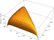
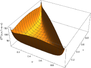
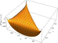
Figure 3: Three-dimensional plots of the finite functions $\mathcal{E}^{(L)}_{3}$ at one, two, and three loops in region (6).

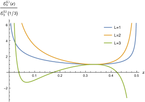
Figure 4: Two-dimensional plots of the finite remainder function $\mathcal{E}^{(L)}_{3}$ up to three loops in the slice $u=v=z$ with $z\in(0,1/2)$ of region (6). Boundaries on the plot correspond to the soft limit ($z\to 0$) and the collinear limit ($z\to 1/2$), as explained in the text.

4.4 Analytic properties

Analytic calculations from bootstrapping approaches of the finite remainder $\mathcal{E}_{2}^{(L)}$ up to eight loops (with $L=8$), and the analytic calculation of the two-loop finite remainder $\mathcal{E}_{3}^{(2)}$ show that these symbol expressions exhibit dependence only on letters of the alphabet,

$$\vec{\alpha}_{u}=\left\{u,v,w,1-u,1-v,1-w\right\}\,.$$ (38)

This alphabet has explicitly appeared in the analytic calculation of four-point two-loop Feynman integrals with one off- and three on-shell external states, giving raise to two-dimensional harmonic polylogarithms (2dHPL’s) Gehrmann:2000zt; Gehrmann:2001ck. For the calculation of three-loop Feynman integrals, however, it was observed that the alphabet (38) needs to be extended for particular integral families Henn:2023vbd. Therefore, it is interesting to ask: will higher-loop contributions to the form factor contain letters of the six-letter alphabet (38) only? We answer this question by studying the analytic properties of the three-loop finite remainder $\mathcal{E}_{3}^{(3)}$.

With the analytic expression of the finite remainder $\mathcal{E}^{(3)}_{3}$ at hand, we can identify the following properties:

1. The first entry of the symbol of $\mathcal{E}^{(3)}_{3}$ always corresponds to an element of the set $\{u,v,w\}$, which is consistent with physical thresholds for massless processes, $s_{ij}=0$ or $q^{2}=0$.

2. The last entry of the symbol of $\mathcal{E}^{(3)}_{3}$ corresponds to an element of the set $\{u/v,v/w,w/u\}$.

3. The symbol of $\mathcal{E}^{(3)}_{3}$ is invariant under the action of the dihedral group, generated by the transformations,

   cycle: $$u\to v\to w\to u\,,$$

   flip: $$u\leftrightarrow v\,.$$ (39)

4. The symbol of $\mathcal{E}^{(3)}_{3}$ satisfies a set of six adjacency restrictions, which, in the alphabet $\vec{\alpha}_{u}$, corresponds to the condition that certain pairs of letters never appear in adjacent positions,

   $$\cancel{\ldots\left(1-u\right)\otimes\left(1-v\right)\ldots}\,, \cancel{\ldots\left(1-v\right)\otimes\left(1-u\right)\ldots}\,,$$

   $$\cancel{\ldots\left(1-u\right)\otimes\left(1-w\right)\ldots}\,, \cancel{\ldots\left(1-w\right)\otimes\left(1-u\right)\ldots}\,,$$

   $$\cancel{\ldots\left(1-v\right)\otimes\left(1-w\right)\ldots}\,, \cancel{\ldots\left(1-w\right)\otimes\left(1-v\right)\ldots}\,.$$ (40)

In order to elucidate further physical constraints for the symbol of $\mathcal{E}^{(3)}_{3}$, we use an alternative symbol alphabet, as carried out in the bootstrapping calculation of $\text{tr}\,\phi^{2}$ to eight loops Dixon:2021tdw. This alphabet is denoted by,

$$\vec{\alpha}_{a}=\{a,b,c,d,e,f\}\,,$$ (41)

with,

$$a=\frac{u}{vw}\,, b=\frac{v}{wu}\,, c=\frac{w}{uv}\,,$$

$$d=\frac{1-u}{u}\,, e=\frac{1-v}{v}\,, f=\frac{1-w}{w}\,.$$ (42)

In this representation, the generators of the dihedral group are understood as,

cycle: $$\left\{a,b,c,d,e,f\right\}\to\left\{b,c,a,e,f,d\right\}\,,$$

flip: $$\left\{a,b,c,d,e,f\right\}\to\left\{b,a,c,e,d,f\right\}\,,$$ (43)

and the adjacency restrictions (40), discussed in iv, correspond to,

(44)