Rotational excitation in sympathetic cooling of diatomic molecular ions by laser-cooled atomic ions

Abstract

Sympathetic cooling of molecular ions through the Coulomb interaction with laser-cooled atomic ions is an efficient tool to prepare translationally cold molecules. Even at relatively high collisional energies of about 1eV (T$\sim$10000K), the nearest approach in the ion-ion collisions never gets closer than $\sim$1nm such that naively perturbations of the internal molecular state are not expected. The Coulomb field may, however, induce rotational transitions changing the purity of initially quantum state prepared molecules. Here, we use estimates of rotational state changes in collisions of diatomic ions with atomic ions (arXiv:1905.02130) and determine the overall rotational excitation accumulated over the sympathetic cooling. We also estimate the cooling time, considering both a single atomic ion and a Coulomb crystal of atomic ions.

I Introduction

Sympathetic cooling of molecular ions by means of co-trapped laser-cooled atomic ions Mølhave and Drewsen (2000); Bowe et al. (1999) is an efficient method for creating cold and ultra-cold molecular ions. Since cooling is mediated by the mutual Coulomb repulsion between the ions, it is independent of the details of the internal structure of the ions, and is therefore generally applicable. Consequently, it has been applied to a wide range of different species, including various polar Mølhave and Drewsen (2000); Koelemeij et al. (2007); Staanum et al. (2008); Willitsch et al. (2008); Hansen et al. (2012) and apolar Blythe et al. (2005); Tong et al. (2010) diatomic molecular ions, and also polyatomic molecular ions  Ostendorf et al. (2006); Højbjerre et al. (2008), some of which have been successfully cooled down to temperatures of some tens of millikelvin. The study of such molecular ions is currently a vivid research topics with applications in e.g., quantum logic protocols Shi et al. (2013); Sinhal et al. (2020), fundamental physics Schiller and Korobov (2005) and cold and ultra-cold chemistry Dulieu and Osterwalder (2018).

Cooling of both the translational and internal degrees of freedom is of great interest in this respect. Indeed, sympathetic cooling by one laser-cooled atomic ion can cool one molecular ion to the ground state of the ion pair within the trap Wan et al. (2015); Rugango et al. (2015); Wolf et al. (2016); wen Chou et al. (2017); Poulsen (2011). Rotationally cold molecular ions is a versatile tool on which to implement quantum technologies. Polar molecular ions benefit from their permanent dipole interaction, which allows for effective control over the molecular ion and has been used to implement various quantum technologies Schuster et al. (2011); Shi et al. (2013); Lin et al. (2020); Chou et al. (2017). A drawback with polar molecular ions is that they may couple to the black body radiation via their dipole moments. A way around this issue is to utilize apolar molecular ions Sinhal et al. (2020), which lack a permanent dipole moment. Molecular ions can also be combined into hybrid systems with neutral species for a wide range of applications in quantum technology and fundamental physics Deiß et al. .

Single molecular ions have even been cooled to the ground state of their collective motion with a single co-trapped and laser-cooled atomic ion Wan et al. (2015); Rugango et al. (2015); Wolf et al. (2016); wen Chou et al. (2017), where various forms of quantum logic spectroscopy Schmidt et al. (2005) have recently been demonstrated Schmidt et al. (2005); Sinhal et al. (2020) and already provided unprecedented spectral resolution. Simultaneously, optical pumping Vogelius et al. (2002); Staanum et al. (2010); Schneider et al. (2010); Deb et al. (2013), helium buffer gas cooling Hansen et al. (2014), probabilistic state preparation Wolf et al. (2016); wen Chou et al. (2017) and resonance enhanced multi-photon ionization (REMPI) Tong et al. (2010); Gardner et al. (2019) have been applied to produce molecular ions in specific internal states with high probability. The latter method differs from the others in that the internal quantum state is prepared prior to sympathetic translational cooling and may thus be prone to state changes during cooling. So far, it has only been applied to form state-selected N${}_{2}^{+}$ molecular ions in the vicinity of the trap potential minimum Tong et al. (2010). This is, however, not practical in general, for example in cases where the neutral precursor molecule (such as H₂ or HD) reacts efficiently with the laser-cooled atomic ions. In such cases, it can be favorable to first produce the state-selected molecular ions in one trap and transfer them into another trap more suitable for translational sympathetic cooling. A similar situation is encountered for molecular ions that have to be produced by an external source, such as an electrospray ion source combined with an internal state pre-cooling trap Stockett et al. (2016). In all these cases, the initial kinetic energy of the captured molecular ions can be as high as the effective trap potential, typically in the $1-10\,$eV range.

One potential issue with sympathetic cooling of molecular ions arises from the Coulomb field, originating from the atomic coolants, may also couple to the rotational degree of freedom and thereby induce rotational state changes during the scattering events of the cooling process Berglund et al. .

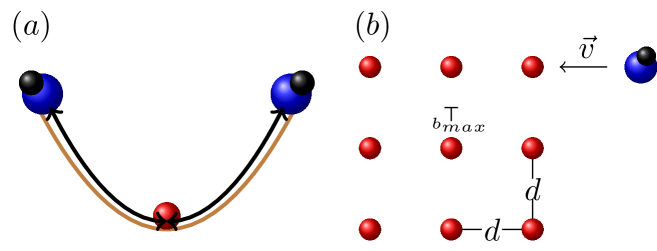
Figure 1: Sympathetic cooling of a molecular ion via collisions with laser-cooled atomic ions: The considered cooling scenarios with either a single trapped atom (a) or many atomic ions forming a Coulomb crystal (b).

Here, we consider sympathetic cooling of diatomic molecular ions with emphasise on the translational cooling dynamics and rotational state excitations. We investigate the feasability of cooling depending of the interatomic distances of the atomic ions in the trap. Additionally, we also estimate the accumulated rotational population excitation probability for initial scattering energies, based on the excitation probability for rotatoinal excitation in a single collision Berglund et al. .

II Translational cooling

Our model is built on a separation of energy scales for translational and internal molecular motion: While initial collisional energies range from $0.1\,$eV to 10 eV, the rotational energy scale is only of the order of $10^{-4}\,$eV, so we can treat the translational dynamics without having to worry about changes in collisional energies due to rotational excitations and vice versa. We inspect two sympathetic cooling regimes, illustrated in Fig. 1(a) and (b), respectively. In both cases, we assume the ion trap potential to be harmonic and isotropic, and either contain a single atomic ion Staanum et al. (2008); Hansen et al. (2012); Tong et al. (2010) (a) or many atomic ions in the form of a Coulomb crystal Staanum et al. (2010); Heazlewood and Softley (2015) (b), which we for simplicity will assume has a simple cubic structure (though often fcc or bcc). As we shall see, the specific scenario will be important for the time required to reach the final energy.

Treating the molecular ion as a point particle, the relative motion reduces to the textbook problem of classical scattering in a $1/r$-potential Goldstein (1980). This neglects the trap potential which is reasonable at the relevant short distances where effective translation energy exchange take place.

Classical scattering is characterized by the scattering energy $E$ and the impact parameter $b$ and the reduced mass $\mu=\frac{m_{mol}M_{at}}{M_{mol}+M_{at}}$ the reduced mass with $M_{mol}$ and $M_{at}$ the molecular and atomic masses. The impact parameter is not fixed, nor controllable, in a sympathetic cooling experiment. We thus need to average over all possible values of $b$. In the following, we focus on two extreme situations—cooling by a single atom (SA) and a large Coulomb crystal (CC). In the SA case, as soon as the atomic ion reach millikelvin temperatures it will remain close to the trap minimum. Consequently, we assume the atom all the time to be in the centre of the trapping potential. Assuming furthermore that the energy E is not fixed, but rather represent a thermal energy distribution with the mean value E, then due to the isotropic trapping potential the distribution of impact parameters is given by

$$f_{SA}(b)=\frac{b}{\sigma^{2}}e^{-\frac{b^{2}}{2\sigma^{2}}}\,,$$ (1)

where $\sigma=\sqrt{E/\left(\mu\omega^{2}\right)}$ is the effective length of the trap at a given energy, $\omega$ the trap frequency. In the second scenario, that of a large Coulomb crystal (CC), the lattice spacing $d$ determines the maximum impact parameter in a scattering event, i.e., $b_{max}=d/2$. Assuming the molecular ion is entering along the [100] direction of the simple cubic lattice, cf. Fig. 1(c), we approximate the impact parameter distribution by

$$f_{CC}(b)=\frac{8b}{d^{2}},\quad b\in[0,\frac{d}{2}]\,.$$ (2)

The translational energy transferred from the molecular ion to the atom (in the laboratory frame) in a single scattering event, $\delta E_{lab}$, is given by

$$\delta E_{lab}=\frac{2\xi(1-\cos{\theta_{sc}})}{(1+\xi)^{2}}E_{lab}\,,$$ (3)

where $E_{lab}$ is the initial collisional energy, $\xi=M_{mol}/M_{at}$ is the molecule to atomic mass ratio, and $\theta_{sc}$ is the scattering angle. The latter depends on the scattering energy $E$ (in the center-of-mass (CM) frame), the impact parameter $b$, and the charges $q_{at}$, $q_{mol}$ of the atomic and molecular ions respectively, in the following way $\theta_{sc}(E,b)=2\sin^{-1}{\left(1/\sqrt{1+\left(\frac{2Eb}{q_{at}q_{mol}}.\right)^{2}}\right)}$.

The CM and lab frame energies are related by

$$E_{lab}=EM_{mol}/\mu$$ (4)

for elastic collisions. Eq. (4) allows us to express the energy transfer, Eq. (3), in the CM frame. The energy transfer relative to the scattering energy in the CM-frame per collision is plotted in Fig. 2 as a function of the impact parameter. We see that the energy transfer is more efficient for scattering pairs with similar masses. In addition, the translational energy transfer per scattering energy for non-head-on collisions increases with decreasing scattering energy.

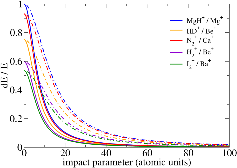
Figure 2: The translational energy transfer, normalized to scattering energy as a function of the impact parameter $b$ for for two scattering energies $E=2$eV (solid lines) and $E=1$ eV (dashed dotted lines) as measured in the CM frame.

A complete cooling process consists of a series of such collisions, and will successively lower the translational energy of the molecular ion. Let the initial and final translational energies of the molecular ion be $E_{max}$ and $E_{min}$ respectively. For a given scattering energy, the typical transfer of kinetic energy from the molecular ion to the coolant, $\Braket{\delta E}$, is given by the average with respect to the impact parameter

$$\Braket{\delta E(E)}=\int_{0}^{\infty}\delta E(E,b)\,f(b)\,db\,,$$ (5)

where the probability distribution $f(b)$ depends on the specific cooling scenario. The distribution function, $f(b)$, for the single ion- and crystal cooling scenarios are obtained from Eqs. (1) and (2) respectively. The total energy transferred in a cycle of $N$ collisions is then

$$\Delta E=E_{max}-E_{min}=\sum_{n=0}^{N-1}\Braket{\delta E}(E_{n}),$$ (6)

where $E_{n+1}=E_{n}-\Braket{\delta E(E_{n})}$. If the energy transfer in each collision is very small compared to the collision energy, then the energy transfer is approximately constant over several collisions, $n(E_{i})$. It is convenient to partition the full energy interval ($E\in[E_{max},E_{min}]$) into $N$ sub intervals such that

$$E_{max}=E_{0}>E_{1}>...\,E_{i}>E_{i+1}>...\,E_{N}=E_{min}$$ (7)

and, assuming that the energy interval $\Delta E_{i}\equiv E_{i}-E_{i+1}$ is not too large,

$$\Delta E_{i}\approx n(E_{i})\Braket{dE}(E_{i})\Rightarrow n(E_{i})\approx\frac{\Delta E_{i}}{\Braket{\delta E}(E_{i})},$$ (8)

thus defining $n(E_{i})$. We can now rewrite Eq. (6) as

$$\Delta E=\sum_{i=0}^{N-1}\Delta E_{i}\approx\sum_{i=0}^{N-1}n(E_{i})\Braket{\delta E}(E_{i}).$$ (9)

We now specify to the particular scenarios considered, beginning with the CC scenario, i.e. cooling by an infinite Coulomb crystal, where, by Eq. (2), the mean energy loss becomes

$$\begin{aligned} \Braket{\delta E(E)}_{CC}&=\frac{8}{d^{2}}\int_{0}^{\frac{d}{2}}\delta E(E,b)bdb,\\ &=\frac{4\xi\log{((d\cdot E)^{2}+1)}}{(1+\xi)^{2}d^{2}E}\,.\end{aligned}$$ (10)

With Eqs. (8) and (10), we have an expression for the number of collisions required to reduce the scattering energy from $E_{i}$ to $E_{i+1}$

$$n(E_{i})_{CC}\approx\frac{(1+\xi)^{2}d^{2}E_{i}}{4\xi\log{((d\cdot E_{i})^{2}+1)}}\Delta E_{i}\,.$$ (11)

We can estimate the time between collisions,

$$\tau_{CC}=\frac{d}{v_{lab}}=d\sqrt{\frac{M_{mol}}{2E_{lab}}}=d\sqrt{\frac{\mu}{2E}},$$ (12)

where $v_{lab}$ is the speed of the molecular ion in the lab frame. Therefore the cooling time on a given subinterval, $i$ is the product of Eqs. (11) and (12). Summing over all subintervals leads to the total cooling time

$$T_{CC} \approx\frac{(1+\xi)^{2}d^{3}}{4\xi}\sqrt{\frac{\mu}{2}}\sum_{i=0}^{N-1}\frac{\sqrt{E_{i}}}{\log{((d\cdot E_{i})^{2}+1)}}\Delta E_{i}$$ (13)

$$\to\frac{(1+\xi)^{2}d^{3}}{4\xi}\sqrt{\frac{\mu}{2}}\int_{E_{min}}^{E_{max}}\frac{\sqrt{E}dE}{\log{((d\cdot E)^{2}+1)}}\,,$$

where the integral is the limit where $\Delta E_{i}\to dE$.

In the SI cooling case with $\sigma$ in Eq. (1) large compared to any $b$ at which energy transfer is significant, we find

$$\Braket{\delta E(E)}_{SA} = \frac{1}{\sigma^{2}}\int_{0}^{\infty}\delta E(E,b)be^{-\frac{b^{2}}{2\sigma^{2}}}db,$$ (14)

$$< \frac{\xi\log{((2\sigma E)^{2}+1)}}{(1+\xi)^{2}\sigma^{2}E}.$$

Using Eq. (14), the number of scattering events required to change the translational energy of the molecular ion by $\Delta E_{i}$ is given by

$$n_{SA}(E_{i}) \approx\frac{\Delta E_{i}}{\Braket{\delta E(E_{i})}}_{SA}$$ (15)

$$>\frac{(1+\xi)^{2}\sigma^{2}E_{i}}{\xi\log{((2\sigma E_{i})^{2}+1)}}\Delta E_{i}.$$

Since the molecular ion will oscillate in the trap, the time between two scattering events amounts to $\tau_{SA}=\frac{\pi}{\omega}$, independent of $E$. By this approximation we essentially neglect the fact that the Coulomb scattering cross section is infinite. Discretizing the energy range, the total time needed to lower the molecular ion’s energy by $\Delta E$ can be approximated by

$$T_{SA} \approx\sum_{i=0}^{N-1}n_{SA}(E_{i})\tau_{SA}=\frac{\pi}{\omega}\sum_{i=0}^{N-1}n_{SA}(E_{i})$$ (16)

$$>\pi\sqrt{\mu}\sum_{i=0}^{N-1}\frac{(1+\xi)^{2}\sigma_{i}^{3}\sqrt{E_{i}}}{\xi\log{((2\sigma_{i}E_{i})^{2}+1)}}\Delta E_{i}$$

with $\sigma_{i}=\sqrt{\frac{E_{i}}{\mu\omega^{2}}}$. From Eq. (16), it is clear that cooling at the highest energies is much slower than at low energies. As a matter of fact, one can estimate an average value for $\tilde{\sigma}\approx\frac{6}{7}\sigma(E_{max})$, where the full evaluation can be found in Appendix A. We may therefore approximate the total cooling time,

$$T_{SA}>\pi\sqrt{\mu}\tilde{\sigma}^{3}\sum_{i=0}^{N-1}\frac{(1+\xi)^{2}\sqrt{E_{i}}}{\xi\log{((2\tilde{\sigma}E_{i})^{2}+1)}}\Delta E_{i}.$$ (17)

We can thus establish a simple relation between the cooling times in the two regimes from Eqs. (17) and (13), namely

$$\frac{T_{SA}}{T_{CC}}\sim\left(\frac{\tilde{\sigma}}{d}\right)^{3}\,.$$ (18)

For standard Coulomb crystals, $d\approx 10\,\mu$m, whereas $\sigma(E_{0})=635\,\mu$m for $E=2\,$eV. With $\omega=2\pi\times 1\,$MHz, $T_{SA}$ is more than $10^{6}$ times larger than $T_{CC}$. As an example, cooling ²⁴MgH⁺ from $2\,$eV to $0.01\,$eV in a crystal of ²⁴Mg⁺ with $d=5.29\,\mu$m takes approximately $2\,$ms in agreement with an earlier estimate Bussmann et al. (2006), compared to $\sim$$40\,$min when cooling with a single atomic ion. Sympathetic translational cooling is thus much more advantageous with a Coulomb crystal.

In order to validate our model for sympathetic cooling in the CC regime, we compare the estimated cooling times obtained from our model with cooling times obtained from molecular dynamics (MD) simulations. The comparison is presented in Table 1. Given the many simplifications and approximations in our model, the results from our model are in strikingly good agreement with the full MD simulations, and tell us that our model is indeed useful.

$n$	$\braket{\delta E_{lab}}$ (eV)	$n_{coll}$	$T_{CC}$ (ms)	$T_{MD}$* (ms)
$10$	$1.15\cdot 10^{-5}$	$3.47\cdot 10^{4}$	$3.53\cdot 10^{-1}$	$\approx 4.6\cdot 10^{-1}$
$20$	$4.80\cdot 10^{-5}$	$8.34\cdot 10^{3}$	$8.48\cdot 10^{-2}$	$\approx 1.3\cdot 10^{-1}$
$30$	$1.14\cdot 10^{-4}$	$3.50\cdot 10^{3}$	$3.56\cdot 10^{-2}$	$\approx 6.0\cdot 10^{-2}$
$40$	$2.11\cdot 10^{-4}$	$1.89\cdot 10^{3}$	$1.93\cdot 10^{-2}$	$\approx 3.6\cdot 10^{-2}$

Table 1: Comparison of the cooling time in the crystal cooling scenario, as obtained by molecular dynamics (MD) simulations and by our model. In the comparison the scattering pair ²⁴MgH⁺-²⁴Mgⁿ⁺, where $n$ is the charge of the atomic ion, is used along with the starting energy $E_{max}=0.4$ eV and $E_{min}=0.0$ eV, in the lab frame. In the flat distribution, the cutoff is $d=17.5$ $\mu$m. The collision frequency was estimated from the initial speed and mean free path and found to be $\approx 280$ MHz. $T_{CC}$ was calculated using one term in the series expansion in Eq. (13). In order to use the equation we also need to specify the average energy transfer in a single collision, $\Braket{\delta E_{lab}}$, Eq. (10), as well as the number of collisions, $n_{coll}$, Eq. (11). *$T_{MD}$ corresponds to the time obtained in ref. Bussmann et al. (2006).

One could wonder if local disruption of the crystal structure and heating effects due to collisions may have a significant effect on subsequent collisions, however, since the speed of sound is typically of the order of $\sim 10m/s$, the ions will during most of the cooling process be moving with supersonic velocities, and previous collisions can have no effect as long the crystal is long enough to stop the incoming ion by passing through once. Even if this is not the case, the mean density cold ions will not change dramatically after passing of a fast ion, and the crystal will be essentially the same before the next passage.

III Rotational excitation during the cooling process

Just as with the kinetic energy transfer, the rotational excitation depends on the scattering energy and the impact parameter. Let the rotational excitation at a given energy and impact parameter be $\epsilon(E,b)$ In order to estimate the rotational excitation over a complete cooling cycle, we discretize the range from the initial to the final scattering energy, analogously to Eq. (13). Just like in the treatment of the translational cooling, we need to average over the impact parameter. We are now only concerned with the crystal cooling scenario, so we use the distribution function in Eq. (2), obtaining $\tilde{\epsilon}(E)=\Braket{\epsilon(E,b)}_{CC}$. If the accumulated cycle excitation is to be small, then certainly $\epsilon(E,b)$ need be small, and since most excitation takes place for impact parameters much smaller than $d$ Berglund et al. , we must have $\tilde{\epsilon}(E)\ll 1$. Once we have obtained $\tilde{\epsilon}(E_{i})$ corresponding to the energy of subinterval $i$, we can estimate the accumulated rotational excitation on this interval by $n(E_{i})\tilde{\epsilon}(E_{i})$. The accumulated rotational excitation in a complete cycle is obtained by summing up the contributions from the subintervals

$$\Phi_{\Sigma}\approx\sum_{i=0}^{N-1}n(E_{i})\tilde{\epsilon}(E_{i})\,.$$ (19)

Notice that Eq. (19) disregards de-excitations that might occur in a multiple scattering sequence. However, this effect will be minor as long as the degree of excitation during the complete translational cooling cycle is much smaller than 1 as assumed above.

In order to obtain the accumulated excitation we need to first to estimate the single collision excitation, $\tilde{\epsilon}(E)$. Since it fundamentally depends on whether it is a polar and apolar molecular ion that is sympathetically cooled, in the following we consider the two cases separately.

III.1 Apolar molecular ions

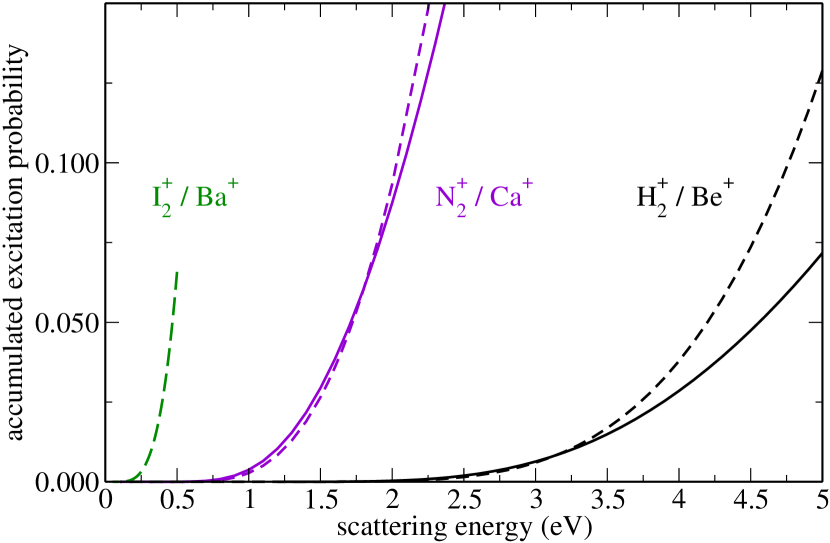
Figure 3: Accumulated excitation for apolar molecular ions after a complete cooling cycle as function of the initial scattering energy, comparing full numerical calculations (dashed lines) to PT (solid lines, $d\approx 5.3$ $\mu$m).

For apolar molecular ions, we calculate numerically the population excitation taking the polarizability and quadrupole interactions into account Berglund et al. . By comparing not only the final excitation, but also the population as a function of time during a collision, we find that an estimate for the rotational excitation after one collision can be obtained as a function of the scattering energy and the impact parameter using first-order time-dependent perturbation theory (PT) Berglund et al. . We find that the quardupole interaction with the field due to the atomic ion coolant dominates the polarizability interaction (i.e. the polarizability contributes much less population excitation for the scattering energies relevant here) and we can therefore neglect the polarizability contribution in our PT-treatment Berglund et al. . For a full cooling process we need to calculate the accumulated rotational excitations by averaging over the impact parameter. In particular, we are interested in calculating averages for the excitations in a single collsions at a fixed scattering energy. In our model, the only quantity in the expression for the single collision excitation that depends on the impact parameter is the third power of the maximum field strength Berglund et al. ,

$$\varepsilon_{0}^{3}(E,b)=\frac{1}{\left(\frac{1}{2E}+\sqrt{\left(\frac{1}{2E}\right)^{2}+b^{2}}\right)^{6}}.$$ (20)

In the CC-scenario, we use Eqs. (2) and (20) to calculate the average

$$\frac{8}{d^{2}}\int_{0}^{\frac{d}{2}}\varepsilon_{0}^{3}(E,b)b\,db\approx\frac{6}{5d^{2}}E^{4}\,.$$ (21)

where the evaluation is presented in Appendix B. From this average we have now obtained an estimate for the population excitation at a given scattering energy in terms of the reduced mass, the lattice spacing, the rotational constant, $B$ and the quadrupole moment along the molecular axis, $Q_{Z}$,

$$\tilde{\epsilon}(E)\approx\left\langle\left|c_{2,0}^{(1)}(E)\right|^{2}\right\rangle \approx 1.86^{2}\frac{1}{150d^{2}}\left(\frac{3Q_{Z}}{4}\right)^{2}\mu E\left(1+6\cdot 1.86\sqrt{\frac{\mu}{E^{3}}}B\right)e^{-6\cdot 1.86\sqrt{\frac{\mu}{E^{3}}}B}.$$ (22)

This expression for the typical rotational excitation in a single collision, together with Eqs. (11) and (19) are what we need to estimate the accumulated cycle excitation. If we let the energy partition become infinitesimal, i.e. let $\Delta E_{i}\to dE$ in Eq. (11), then the sum in Eq. (19) becomes an integral,

$$\Phi_{\Sigma} \approx 1.86^{2}\frac{3(1+\xi)^{2}\mu Q_{Z}^{2}}{200\xi}\times$$

$$\int_{E_{i}}^{E_{f}}\frac{E^{2}\left(1+6\cdot 1.86\sqrt{\frac{\mu}{E^{3}}}B\right)e^{-6\cdot 1.86\sqrt{\frac{\mu}{E^{3}}}B}}{\log{\left(\left(d\cdot E\right)^{2}+1\right)}}dE\,.$$

which is our final result for apolar molecular ions. The final estimate for the accumulated excitation probability at the end of the cooling process nearly only depends on the molecular parameters and initial scattering energy, where the dependence on the lattice splitting is weak due to the logarithm.

In Fig. 3, numerical and analytical results are presented for a few selected combinations of molecular and atomic ion species. For the popular example of N${}_{2}^{+}$ - Ca⁺ Tong et al. (2010); Germann et al. (2014); Germann and Willitsch (2016a, b), we expect excitation of more than a few percent only for initial scattering energies well above 1.5 eV (CM). However, for very heavy molecular ions with small rotational constants, such as I${}_{2}^{+}$, significant rotational excitation is expected already for initial energies of a few hundred meV. At the other end we find the scattering pair H${}_{2}^{+}$ - Be⁺, representing a molecular ion with a large rotational constant. In this case we observe a resilience to rotational excitations, our results indicate that significant excitations above a few procent to occur above 3.5 eV (CM). Notie that the discrepancy between analytical and numerical results for higher energies are more significant for H${}_{2}^{+}$ than for N${}_{2}^{+}$. The reason for this is our neglect of the polarizability interaction for the analytical calculations. The polarizability becomes more important for high energies, and the polarizability interaction is relatively more pornounced for H${}_{2}^{+}$ Berglund et al. . In Fig. 3 we have assumed $d=5.3$ $\mu$m . However, since the main contribution to both the sympathetic cooling process and the rotational excitations take place at very much shorter distances, neither d nor actually the cooling scenario are important for the complete cooling cycle result. The total cooling time, however, strongly depends on the particular scenario and values of $d$ as explained above.

III.2 Polar molecular ions

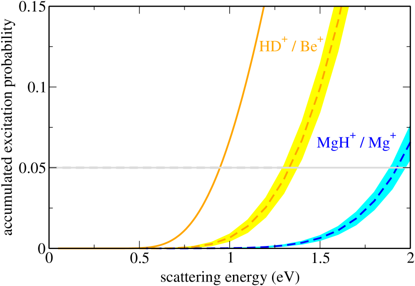
Figure 4: Accumulated excitation probability, Eq. (19), for polar molecular ions after a complete cooling cycle, as a function of the initial scattering energy with $E_{final}=0.1\,$eV, comparing the estimate (solid lines) based on approximation (25) (with $\delta E=0.05\,$eV) to full numerical simulations (dashed lines, $\delta E=0.1$ eV). Within each interval $\delta E$, the excitation occurring in a single collision, $\tilde{\epsilon}$, can be evaluated at the highest and lowest energy, $E_{i}$ and $E_{i}-\delta E$, defining the shaded region, or taken to be the arithmetic mean, indicated by the dashed lines. The horizontal gray line marks an excitation level of 5%.

For the polar case, the dominant interaction between the molecular ion and the electric field originating on the coolant atomic ion is the dipole interaction, which is linear in the electric field strength. This combined with the gradual variation of the Coulomb interaction at large distances leads to a slow onset (offset) of the interaction between the two scattering ions as they approach (receed). This in turn allows for the single collision dynamics to be analyzed in the adiabatic picture, as done in Ref. Berglund et al. . In general, the scattering is in the high field limit, leading to strong following of the field, and no closed formula can be found for $\tilde{\epsilon}(E)$. However, for molecular ions having a low permanent dipole moment, the effect of the field on the rotational states is moderate, and an approximate, two-level model can be used, which leads to the following expression for $\epsilon(E_{i})$ Berglund et al. :

$$\tilde{\epsilon}(E)=\frac{(1.86\pi D)^{2}\mu}{6E^{3}b_{max}^{2}}\int_{0}^{b_{max}}\frac{\exp{\left(-2\cdot 1.86B\sqrt{\frac{\mu}{E^{3}}}\sqrt{1+\frac{D^{2}}{3B^{2}\left(\frac{1}{2E}+\sqrt{\left(\frac{1}{2E}\right)^{2}+b^{2}}\right)^{4}}}\right)}}{\left(\frac{1}{2E}+\sqrt{\left(\frac{1}{2E}\right)^{2}+b^{2}}\right)^{4}+\frac{D^{2}}{3B^{2}}}b\,db.$$ (24)

From this we estimate the accumulated excitation in a complete cooling cycle using Eq. (19) to be

$$\Phi_{\Sigma} \approx\sum_{i=1}^{N}n(E_{i})\tilde{\epsilon}(E_{i})$$ (25)

$$\approx\frac{\left(1+\xi\right)^{2}d^{2}}{4\xi}\sum_{i=1}^{N}\frac{E_{i}\tilde{\epsilon}(E_{i})}{\log{\left(d\cdot E_{i}\right)^{2}+1}}\Delta E_{i}$$

The accumulated excitation is presented in Figure 4. Here we present both analytical and numerical results for HD$~{}+$, representing the low-field limit, and only numerical results for MgH⁺,representing the high-field limit. For the low-field limit (orange) our estimate, Eq. (25) is in fair agreement with the numerical results, but not as well as for the apolar case. We notice that our estimate gives an upper bound to the numerical results at relevant scattering energies. We attribute this effect, in part, because single collisions tends to give an upper bound for low energies and high values of the impact parameters, where the effect of the field is weak Berglund et al. . Notice also that the averaging process, Eq. (24) suppresses the value of the integral at low impact parameters, due to the differential elemment, $b\,db$. This resoning fails at higher energies, as can be seen in Figure 4, but at such high energies the probability excitation is so high that an estimate is no longer relevant. In the high-field limit we have no estimate for the single excitation Berglund et al. , and we can therefore not estimate the full cycle either. A high dipole moment does suppress the rotational excitation process Berglund et al. , a fact that is reflected in the low accumulated excitation probability seen in the figure, and we can therefore expect, contraintuitively, that a molecular ion with a high permanent dipole moment should be resilient against rotational excitations in a sympathetic cooling process. The accumulated excitations obtained from numerical calculations of single collision excitations predict a total excitation of $0.05$ at $E\approx 1.8,1.25$ eV for MgH⁺ and HD⁺ respectively. By Eq.(4) these energies correspond to $E_{lab}\approx 3.5,1.6$ eV for MgH⁺ and HD⁺ respectively. For the apolar species N${}_{2}^{+}$, H${}_{2}^{+}$ and I${}_{2}^{+}$ the corresponding lab energies are $E_{lab}\approx 2.6,4.9,2.8$ eV.

One may wonder if the trapping field also could lead to rotational excitations. The strongest fields are found in rf traps, where the dominating rf-fields can reach maximum amplitudes of $\sim 10^{5}$V/m. For typical values dipole moments of polar diatomic molecular ions, such fields leads to a coupling energy of $\sim 10^{-24}$ Joule or equivalent a frequency of $\sim 1$ GHz. Since this frequency is orders of magnitude lower than the frequencies associated with the rotational splitting in the molecular ions considered above, we do not expect any significant contribution of the trapping fields to rotational state excitations. Notice however that even though the trap field is negligible in terms of the rotational state splitting it can lead to mixing of $m_{J}$-sub-levels Hashemloo and Dion (2015); Hashemloo et al. (2016).

IV Conclusions and outlook

With regards to estimating the rotational excitation in a cooling process, we find the situation to be considerably different for apolar and polar molecular ions respectively. Predicting the rotational excitation of diatomic molecular ions during sympathetic cooling by laser-cooled atomic ions can be estimated in terms of the adiabatic picture for polar molecular ions. The estimate is conservative and not very accurate, in particular for high field (energy) scattering. For polar molecular ions an accurate estimate requires a full quantum-dynamical treatment, whereas validity of PT for apolar molecular ions has allowed us to derive a closed-form estimate of the accumulated population excitation which solely depends on the molecular parameters and initial scattering energy.

The scenarios of using a Coulomb crystal of atomic ions or just a single atomic ion do not significantly change the final degree of collision-induced rotational excitation. However, translational cooling with a single atomic ion is dramatically slower and will generally be impractical.

For a wide range of apolar molecular ions, we find the internal state to be preserved for initial energies of 1 eV and above, eventually limited by close-encounter interactions disregarded in the present treatment. Our result could be of interest to experimentalists for their desing of a particular experimental setup. E.g., if a particular molecular ion is to be used, our estimates can serve as a guide in chosing the trap depth in order to keep rotational excitations under a given threshold. Conversly, if the potential depth is set for a given experiment, our results can serve as a guide indicating which molecular ions are robust enough to serve as systems for the desired application.

When extending the treatment to polyatomics, we expect rotational excitation to be more critical, both because of more degrees of freedom with low-energy spacings and the physical size of the molecules making close-encounter interactions more likely. The latter deserve a more thorough investigation in future work as they might provide a new avenue for controlling collisions due to the extremely large fields present in a close encounter. The control knob would be the initial collision energy which can be varied via the choice of the molecule’s position in the trap during photo-ionization, or by injecting low-energetic molecular ions from an external source into the trap. The same techniques could also be used to experimentally test our present predictions for diatomics.

Appendix A An estimate of an average of $\sigma(E)$ in the single ion cooling scenario

The average of $\sigma(E)=\sqrt{\frac{E}{\mu\omega^{2}}}$ in the single ion cooling scenario, from an initial scattering energy $E_{max}$ to a final scattering energy $E_{min}$, can be estimated by

$$\tilde{\sigma}=\frac{1}{N}\int_{E_{min}}^{E_{max}}\sigma(E)n(E)\,dE,$$ (26)

where the total number of collisions is

$$N=\int_{E_{min}}^{E_{max}}n(E)\,dE$$ (27)

and $n(E)$ is given by Eq. (15), i.e. we will approximate $n(E)\,dE\approx\frac{(1+\xi)^{2}\sigma^{2}E}{\xi\log{((2\sigma E)^{2}+1)}}\,dE$. Since the logarithm changes slowly compared to other factors in the integrand we will treat it as a constant, $\frac{1}{\log{(\tilde{x}^{2}+1)}}$, for some $2\sigma(E_{min})E_{min}<\tilde{x}<2\sigma(E_{max})E_{max}$. With this approximation we arrive at

$$N\approx\frac{\alpha}{3}\left(E_{max}^{3}-E_{min}^{3}\right),$$ (28)

where $\alpha=\frac{(1+\xi)^{2}}{\xi}\frac{1}{\mu\omega^{2}}\frac{1}{\log(\tilde{x}^{2}+1)}$. Now, Eq. (26) becomes

$$\tilde{\sigma}\approx\frac{\frac{2\alpha}{7}\sqrt{\frac{1}{\mu\omega^{2}}}\left(E_{max}^{7/2}-E_{min}^{7/2}\right)}{\frac{\alpha}{3}\left(E_{max}^{3}-E_{min}^{3}\right)}.$$ (29)

Assuming that the lower energy is much smaller than the maximum, or $E_{min}\to 0$, we obtain

$$\tilde{\sigma}\approx\frac{6}{7}\sqrt{\frac{1}{\mu\omega^{2}}}E_{max}^{1/2}=\frac{6}{7}\sigma(E_{max}).$$ (30)

Appendix B Evaluation of $\Braket{\varepsilon_{0}^{3}}_{CC}$

The average of $\varepsilon_{0}^{3}$ Berglund et al. over the impact parameter in the crystal cooling scenario is

$$\Braket{\varepsilon_{0}^{3}}_{CC}=\frac{8}{d^{2}}\int_{0}^{\frac{d}{2}}\frac{b\;db}{\left(\frac{1}{2E}+\sqrt{\left(\frac{1}{2E}\right)^{2}+b^{2}}\right)^{6}}$$ (31)

Let $r=\frac{1}{2E}$. The integral can be evaluated by a symbolic mathematical software program, such as wxmaxima, with the result

$$\Braket{\varepsilon_{0}^{3}}_{CC} =\frac{8}{d^{2}}\int_{0}^{\frac{d}{2}}\frac{bdb}{\left(r+\sqrt{r^{2}+b^{2}}\right)^{6}}$$ (32)

$$=\frac{8}{d^{2}}\left(\frac{-5\left(\frac{d}{2}\right)^{6}+\sqrt{\left(\frac{d}{2}\right)^{2}+r^{2}}\left(24\left(\frac{d}{2}\right)^{4}r+88\left(\frac{d}{2}\right)^{2}r^{3}+64r^{5}\right)-60\left(\frac{d}{2}\right)^{4}r^{2}-120\left(\frac{d}{2}\right)^{2}r^{4}-64r^{6}}{20\left(\frac{d}{2}\right)^{10}}+\frac{3}{320r^{4}}\right)$$

With $\frac{d}{2}\gg r=\frac{1}{2E}$, the main contribution from the first term in the parenthesis is $\left|-\frac{1}{4\left(\frac{d}{2}\right)^{4}}\right|\ll\frac{3}{320r^{4}}$. Therefore,

$$\Braket{\varepsilon_{0}^{3}}_{CC}\approx\frac{8}{d^{2}}\frac{3}{320r^{4}}=\frac{12}{10d^{2}}E^{4}.$$ (33)

References

- Mølhave and Drewsen (2000) K. Mølhave and M. Drewsen, Phys. Rev. A 62, 011401 (2000).
- Bowe et al. (1999) P. Bowe, L. Hornekær, C. Brodersen, M. Drewsen, J. S. Hangst, and J. P. Schiffer, Phys. Rev. Lett. 82, 2071 (1999).
- Koelemeij et al. (2007) J. C. J. Koelemeij, B. Roth, A. Wicht, I. Ernsting, and S. Schiller, Phys. Rev. Lett. 98, 173002 (2007).
- Staanum et al. (2008) P. F. Staanum, K. Højbjerre, R. Wester, and M. Drewsen, Phys. Rev. Lett. 100, 243003 (2008).
- Willitsch et al. (2008) S. Willitsch, M. T. Bell, A. D. Gingell, S. R. Procter, and T. P. Softley, Phys. Rev. Lett. 100, 043203 (2008).
- Hansen et al. (2012) A. K. Hansen, M. A. Sørensen, P. F. Staanum, and M. Drewsen, Angew. Chemie Int. Ed. 51, 7960 (2012).
- Blythe et al. (2005) P. Blythe, B. Roth, U. Fröhlich, H. Wenz, and S. Schiller, Phys. Rev. Lett. 95, 183002 (2005).
- Tong et al. (2010) X. Tong, A. H. Winney, and S. Willitsch, Phys. Rev. Lett. 105, 143001 (2010).
- Ostendorf et al. (2006) A. Ostendorf, C. B. Zhang, M. A. Wilson, D. Offenberg, B. Roth, and S. Schiller, Phys. Rev. Lett. 97, 243005 (2006).
- Højbjerre et al. (2008) K. Højbjerre, D. Offenberg, C. Z. Bisgaard, H. Stapelfeldt, P. F. Staanum, A. Mortensen, and M. Drewsen, Phys. Rev. A 77, 030702 (2008).
- Shi et al. (2013) M. Shi, P. F. Herskind, M. Drewsen, and I. L. Chuang, New Journal of Physics 15, 113019 (2013).
- Sinhal et al. (2020) M. Sinhal, Z. Meir, K. Najafian, G. Hegi, and S. Willitsch, Science 367, 1213 (2020), https://www.science.org/doi/pdf/10.1126/science.aaz9837 .
- Schiller and Korobov (2005) S. Schiller and V. Korobov, Physical Review A 71, 032505 (2005).
- Dulieu and Osterwalder (2018) O. Dulieu and A. Osterwalder, eds., Cold Chemistry: Molecular Scattering and Reactivity Near Absolute Zero (The Royal Society of Chemistry, 2018).
- Wan et al. (2015) Y. Wan, F. Gebert, F. Wolf, and P. O. Schmidt, Phys. Rev. A 91, 043425 (2015).
- Rugango et al. (2015) R. Rugango, J. E. Goeders, T. H. Dixon, J. M. Gray, N. B. Khanyile, G. Shu, R. J. Clark, and K. R. Brown, New J. Phys. 17, 035009 (2015).
- Wolf et al. (2016) F. Wolf, Y. Wan, J. C. Heip, F. Gebert, C. Shi, and P. O. Schmidt, Nature 530, 457–460 (2016).
- wen Chou et al. (2017) C. wen Chou, C. Kurz, D. B. Hume, P. N. Plessow, D. R. Leibrandt, and D. Leibfried, Nature 545, 203 (2017).
- Poulsen (2011) G. Poulsen, Sideband Cooling of Atomic and Molecular Ions, Ph.D. thesis, Department of Physics and Astronomy, Aarhus University (2011).
- Schuster et al. (2011) D. Schuster, L. S. Bishop, I. Chuang, D. DeMille, and R. Schoelkopf, Physical Review A 83, 012311 (2011).
- Lin et al. (2020) Y. Lin, D. R. Leibrandt, D. Leibfried, and C.-w. Chou, Nature 581, 273 (2020).
- Chou et al. (2017) C.-w. Chou, C. Kurz, D. B. Hume, P. N. Plessow, D. R. Leibrandt, and D. Leibfried, Nature 545, 203 (2017).
- (23) M. Deiß, S. Willitsch, and J. Hecker Denschlag, Nature Physics 20, 713.
- Schmidt et al. (2005) P. O. Schmidt, T. Rosenband, C. Langer, W. M. Itano, J. C. Bergquist, and D. J. Wineland, Science 309, 749 (2005), https://www.science.org/doi/pdf/10.1126/science.1114375 .
- Vogelius et al. (2002) I. S. Vogelius, L. B. Madsen, and M. Drewsen, Phys. Rev. Lett. 89, 173003 (2002).
- Staanum et al. (2010) P. F. Staanum, K. Højbjerre, P. S. Skyt, A. K. Hansen, and M. Drewsen, Nature Phys. 6, 271 (2010).
- Schneider et al. (2010) T. Schneider, B. Roth, H. Duncker, I. Ernsting, and S. Schiller, Nature Phys. 6, 275 (2010).
- Deb et al. (2013) N. Deb, B. R. Heazlewood, M. T. Bell, and T. P. Softley, Phys. Chem. Chem. Phys. 15, 14270 (2013).
- Hansen et al. (2014) A. K. Hansen, O. O. Versolato, L. Kłosowski, S. B. Kristensen, A. Gingell, M. Schwarz, A. Windberger, J. Ullrich, J. R. C. López-Urrutia, and M. Drewsen, Nature 508, 76 (2014).
- Gardner et al. (2019) A. Gardner, T. Softley, and M. Keller, Sci. Rep. 9, 506 (2019).
- Stockett et al. (2016) M. H. Stockett, J. Houmøller, K. Støchkel, A. Svendsen, and S. Brøndsted Nielsen, Rev. Sci. Instrum. 87, 053103 (2016).
- (32) J. M. Berglund, M. Drewsen, and C. P. Koch, arXiv:1905.02130 .
- Heazlewood and Softley (2015) B. R. Heazlewood and T. P. Softley, Annu. Rev. Phys. Chem. 66, 475 (2015).
- Goldstein (1980) H. Goldstein, Classical Mechanics (Addison-Wesley, 1980).
- Bussmann et al. (2006) M. Bussmann, U. Schramm, D. Habs, V. Kolhinen, and J. Szerypo, Int. J. Mass Spectrom. 251, 179 (2006).
- Germann et al. (2014) M. Germann, X. Tong, and S. Willitsch, Nature Phys. 10, 820 (2014).
- Germann and Willitsch (2016a) M. Germann and S. Willitsch, J. Chem. Phys. 145, 044314 (2016a).
- Germann and Willitsch (2016b) M. Germann and S. Willitsch, J. Chem. Phys. 145, 044315 (2016b).
- Hashemloo and Dion (2015) A. Hashemloo and C. M. Dion, J. Chem. Phys. 143, 204308 (2015).
- Hashemloo et al. (2016) A. Hashemloo, C. M. Dion, and G. Rahali, Internat. J. Mod. Phys. C 27, 1650014 (2016).