Quasisections of circle bundles and Euler class

Abstract.

Let $E\xrightarrow[\text{}]{\pi}B$ be an oriented circle bundle over an oriented closed surface $B$. A quasisection is a closed smooth manifold ${Q}$ mapped by a generic smooth mapping $q$ to $E$ such that $\pi\circ q({Q})=B$.

In the paper we show that Euler number (Euler class) of the bundle equals the sum of weights of (some of) singularities of a quasisection. We also prove the uniqueness of such a formula.

The formula is a close relative of M. Kazarian’s formula which relates the Euler number and Morse bifurcations of a generic function defined on the total space $E$.

1. Introduction

Let $E\xrightarrow[\text{}]{\pi}B$ be a circle bundle, that is, an oriented locally trivial fiber bundle whose fibers are circles $S^{1}$. Assume that the base $B$ is a closed $2$-dimensional oriented surface. Such bundles are classified by their Euler classes, or just Euler numbers.

Definition 1.

A quasisection of $E\xrightarrow[\text{}]{\pi}B$ is a closed smooth manifold $Q$ and a smooth map $q:Q\rightarrow E$ such that $\pi\circ q(Q)=B$.

The pair $(Q,q)$ will be denoted by $\mathcal{Q}$. We also abbreviate the composition $\pi\circ q:Q\rightarrow B$ as $\pi:{\mathcal{Q}}\rightarrow B$.

Throughout the paper, the maps $q$ and $\pi\circ q$ are assumed to be generic, or stable, in the sense of Whitney’s singularity theory [1]. In particular, this means that the singularities of $q$ can be lines of self-intersection, isolated triple points, and Whitney umbrellas only. We also assume that away from Whitney umbrellas, the singularities of $\pi\circ q$ are pleats and folds. There are some more natural genericity conditions; we discuss them in due time.

Main results

• Theorem 1 (The local formula for the Euler number) asserts that the Euler number of a bundle equals the weighted number of some special singularities of the quasisection, called singular vertices. These are: ($I$) intersections of (projections of) two folds of $\mathcal{Q}$, ($II$) pleats of $\mathcal{Q}$, and ($III$) intersections of a fold and a regular sheet of $\mathcal{Q}$.

• Section 4 gives a zoo of quasisections.

• Theorem 3 (the uniqueness theorem) asserts that no other assignement of weights gives a valid local formula.

Motivations

Let us now mention relatives of our results and some motivations.

In [8], the following construction is used. Given a generic smooth function $f:E\rightarrow\mathbb{R}$, the restriction of $f$ to a fiber has (at least two) critical points. The set of critical points taken over all the fibers is a close analogue of a quasisection, but generic singularities in that framework look different. So what we prove is a very close relative of Theorem 1.4, (4) from [8].

We would also like to mention the local combinatorial formulae for the Euler class, [7, 11], that retrieve the Euler class of the bundle from local data of a triangulated circle bundle. It was proven in [17] that this formula is not unique, so for triangulated bundles the analogue of Theorem 3 does not hold.

Stable maps between closed surfaces have been studied since long. A stable map has folds and pleats only; the fold lines may have self-intersections in the image. There exist some relationships between the Euler characteristics of the surfaces, number of pleats, number (and types) of crosses of the fold in the image, etc. [4, 12, 13]. For instance, it is known [14, 15] that a generic map from $\mathbb{R}P^{2}$ to $\mathbb{R}^{2}$ necessarily has an odd number of pleats.

Theorem 1 can be also considered as a relationship between weighted number of singularities and the Euler class of the fiber bundle. In our formula we have ”old” singularities, (crossings of folds and pleats) counted with some weights, and also ”new” singularities (crossings of a fold and a regular sheet) which are not visible via the map $\pi\circ q$.

A reminder on Euler class

We remind the reader that a circle bundle is uniquely defined by its Euler class $\mathcal{E}(E\rightarrow B)\in H^{2}(B,\mathbb{Z})$. Fixing an orientation of $B$ and identifying $H^{2}(B,\mathbb{Z})$ with $\mathbb{Z}$, we speak of the Euler number $\mathcal{E}$ of a bundle $E\rightarrow B$.

We use the following way to compute the Euler number: Assume that a partial section $s:B\setminus\{x_{i}\}\rightarrow E$ is defined everywhere except for a finite set of points $x_{1},...,x_{m}\in B$. For each of $x_{i}$ take a neighborhood $U_{i}$ bounded by a small circle $C_{x_{i}}$. The circle inherits an orientation from $B$. Next, choose a trivialization of the bundle in the neighborhood $U_{i}$. The restriction of the section $s$ defines a map

$$s_{\mid_{C_{x_{i}}}}:C_{x_{i}}\rightarrow S^{1}.$$

The source and the target are two oriented circles, so the degree of the map is well-defined. Set

$$ind_{s}(x_{i}):=deg\leavevmode\nobreak\ s_{\mid_{C_{x_{i}}}}.$$

The index $ind_{s}(x_{i})$ depends on the section $s$, but the sum of the indices over all $x_{i}$ does not:

Proposition 1.

[9], [3]. In the above notation,

$$\mathcal{E}(E\rightarrow B)=\sum_{i}ind_{s}(x_{i}).$$

Now we can explain the leading idea of our construction in short (it traces back to M. Kazarian’s multisections [8]).

Assume we have a random section $s$ defined outside some fixed finite set $\{x_{i}\}\subset B$. Then one can take the expectation:

$$\mathcal{E}(E\rightarrow B)=\mathbb{E}\Big{(}\sum_{i}ind_{s}(x_{i})\Big{)}=\sum_{i}\mathbb{E}(ind_{s}(x_{i})).$$

We will show that a quasisection yields a random section with a finite probability space. In other words, a quasisection gives a finite collection of partial sections, and taking $\mathbb{E}$ amounts to averaging.

2. Singular points and their portraits

2.1. Singularities

Let $\mathcal{Q}=(Q,q)$ be a quasisection of a circle bundle.The singular curve of $\mathcal{Q}$ is the image under projection $\pi$ of the line of self-intersection, and of folds of $\mathcal{Q}$.

We assume in the paper that singularities of the singular curve are stable, that is, persist under small perturbations of $q$. For instance, (the projections of) two pleats never coincide, there are no triple crossing points of (projections of) folds, etc.

Remark. Stability means that intersection of projections of two folds is always transversal. But the projection of a line of self-intersection may be stably tangent to the projection of a fold. This happens whenever a regular sheet of $\mathcal{Q}$ crosses a fold in $E$.

A singular vertex is one of the following:

1. A self-intersection of the singular curve.

2. The image under projection $\pi$ of a Whitney umbrella.

3. The image under projection $\pi$ of a pleat.

Singular vertices cut the singular curve into singular segments (or singular circles, if a component of the singular curve is closed and has no singular vertices).

A typical landscape of singular curves and singular vertices of a generic quasisection is depicted in Fig. 1.

Figure 1. Singular curve and singular vertices, a fragment of a typical landscape.

2.2. Portraits of points from the base

Let $x\in B$ be an arbitrary point. We may assume that its neighborhood and the preimage of the neighborhood are equipped with flat Riemanian metrics such that the projection $\pi$ locally equals the orthogonal projection, and the fibers have one and the same length. Let $C_{x}$ be a small circle embracing $x$. Then $\pi^{-1}(C_{x})$ is a flat torus. The circle $C_{x}$ is oriented according to the orientation of $B$; the orientation is depicted counterclockwise. We depict $\pi^{-1}(C_{x})$ as an annulus assuming that its inner and the outer circles are glued. Besides, we assume that the orientations of the fibers point inwards, from the outer circle to the inner circle, see Fig. 2, left. In the annulus, we mark $\pi^{-1}(C_{x})\cap\mathcal{Q}$, which is a non-emply union of some curves.

This picture is called the portrait of the point $x\in B$. We say that two portraits are equal if they differ on orientation preserving fiberwise diffeomorphism.

Example.

1. If $x$ is a regular point, its portrait (Fig. 2, left) is a disjoint union of a non-zero number of simple circles. Each simple circle comes from a regular sheet of $\mathcal{Q}$.

2. Assume $x$ belongs to the interior of a singular edge which comes from a fold. Then its portrait looks as is depicted in Fig. 2, right. It consists of a (non-zero) number of simple circles, and one fold curve.

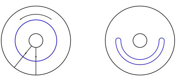
Figure 2. Left: The portrait of a regular point. Right: A portrait of a point $x$ lying on a fold.

It is easy to see:

Lemma 1.

1. If $x$ ranges within the interior of one and the same singular edge (so $x$ is not a singular vertex), its portrait does not change.

2. Portrait of an intersection point of (projections of) two folds is as in Fig. 3, left, up to adding/removing some of simple circles.

   Such a singular vertex is called type $I$.

3. Portrait of a (projection of a) pleat is (up to line symmetry) as in Fig. 3, center. The number of simple circles may vary.

   Such a singular vertex $x$ is called type $II$, right (respectively, left), if its portrait equals to (respectively, is line symmetric to) Fig. 3, center.

4. Portrait of the projection of an intersection of a fold and a regular sheet is (up to line symmetry) as in Fig. 3, right.

   Such a singular vertex $x$ is called type $III$, right (respectively, left) if its portrait equals to (respectively, is line symmetric to) Fig. 3, right, also up to some number of simple circles.

Singular vertices of types $I$, $II$, and $III$ are called essential vertices.

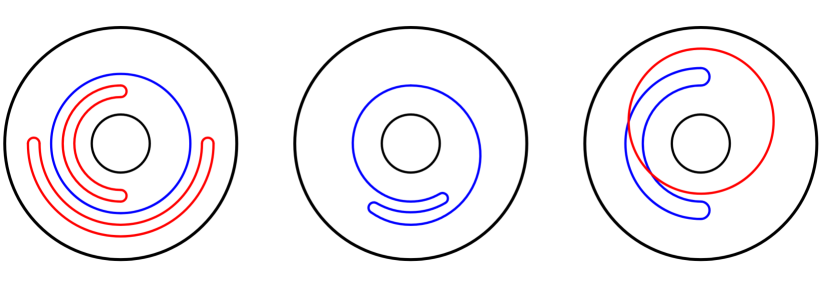
Figure 3. The list of all non-symm portraits, types $I$, $II$ right, and $III$ right.

Now consider the projection of a Whitney umbrella. Let us remind that a Whitney umbrella is defined (in suitable coordinates, and up to diffeomorphisms of the target and the source spaces) as $x(u,v)=uv,\ y(u,v)=u,\ z(u,v)=v^{2}$. The point $W=(0,0)$ is called the endpoint of the umbrella, and the line of self-intersection emanating from $W$ is called the handle.

We are interested in the portrait of (projection of) the endpoint $W$ under assumption that the projection goes in a generic direction.

Lemma 2.

The portrait of a Whitney umbrella is a disjoint union of a number of simple circles and an umbrella curve, as in Fig. 4. Therefore the portrait has a line symmetry. The other scenarios are non-generic.

Proof.

Let $x=\pi(W)$. Since we are interested in the local picture only, assume that we deal with a Whitney umbrella in $\mathbb{R}^{3}$ and with the standard orthogonal projection $\pi$ to the horizontal plane. Take a generic point $p\in C_{x}$ and a plane $h\subset\mathbb{R}^{3}$ which contains the endpoint $W$ of the umbrella, and the points $p$ and $x$. Therefore $h$ contains the direction of the projection (the vertical direction). Denote by $p^{\prime}\in C_{x}$ the point opposite to $p$.

The intersection of a Whitney umbrella with a generic plane passing through $W$ is a planar curve with an $A_{2}$ singularity at $W$, see [5]. It has the following properties : (1) Each vertical line in $h$ which is sufficiently close to $W$, intersects the curve in at most three points. (2) If $\pi^{-1}(p)$ intersects the curve at $3$ points, then $\pi^{-1}(p^{\prime})$ has no intersections with the curve. Now a simple case analysis completes the proof. ∎

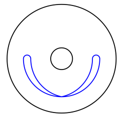
Figure 4. The portrait of a Whitney umbrella

It is easy to check:

Lemma 3.

The portraits of all the singular vertices that are not listed in Lemma 1 have a line symmetry.

Let $x$ be an essential vertex of type $I$.

Imagine a point $y$ that goes along the circle $C_{x}$ in the ccw direction, starting from a place with no fold curves, that is, with the minimal number of points in $\pi^{-1}(y)\cap\mathcal{Q}$. Let us order the folds as follows: the point $y$ meets the first fold first. The other fold is the second.

Now let $n(x)$ be the number of simple circles of $\pi^{-1}(y)\cap\mathcal{Q}$ lying between the first and the second fold curves, if one counts from the first fold curve in the direction of the fiber.

Set also $k(x)$ be the number of simple circles lying between the fold curves, if one counts from the second fold curve in the direction of the fiber.

It is clear that:

Lemma 4.

1. (Two folds intersect in the projection)

   1. The portrait of an essential vertex of type $I$ defines (and is defined by) two numbers, $n$ and $k$.

   2. For the line symmetry image, $n$ and $k$ interchange.

   3. The number $n+k$ cannot be zero.

2. (A pleat) The portrait of an essential vertex of type $II$ defines (and is defined by) its type (right or left) and the number $r$ of simple circles ($r$ might be zero).

3. (A fold intersects a regular sheet) The portrait of an essential vertex of type $III$ defines (and is defined by) its type (right or left) and the number $r$ of simple circles ($r$ might be zero).

Let us assign weights to the essential singular vertices:

Definition 2.

1. For an essential vertex $x$ of type $I$, set

   $$\mathcal{W}_{ff}(x)=\mathcal{W}_{ff}(n,k)=\frac{4(n-k)}{(n+k)(n+k+2)(n+k+4)}.$$

2. For a right essential vertex $x$ of type $II$ set

   $$\mathcal{W}_{p}(x)=\mathcal{W}_{p,R}(r)=\frac{2}{(r+1)(r+3)}$$

   For a left essential vertex $x$ of type $II$ set

   $$\mathcal{W}_{p}(x)=\mathcal{W}_{p,L}(r)=\frac{-2}{(r+1)(r+3)}.$$

3. For a right essential vertex $x$ of type $III$, set

   $$\mathcal{W}_{fs}(x)=\mathcal{W}_{fs}(r,R)=\frac{2}{(r+1)(r+3)}$$

   For a left essential vertex $x$ of type $III$, set

   $$\mathcal{W}_{fs}(x)=\mathcal{W}_{fs}(r,L)=\frac{-2}{(r+1)(r+3)}.$$

3. Local formula for the Euler class

Theorem 1.

The Euler number of a circle bundle with a generic quasisection $\mathcal{Q}$ equals the sum of weights of essential singular vertices:

$$\mathcal{E}=\sum_{I}\mathcal{W}_{ff}(x_{i})+\sum_{II}\mathcal{W}_{p}(x_{i})+\sum_{III}\mathcal{W}_{fs}(x_{i}).$$

That is, only pairwise intersections of folds, pleats, and intersections of a fold and a regular sheet matter.

Proof.

Multisections. The singular curve cuts the base $B$ into open domains $D_{1},...,D_{N}$. For a domain $D_{i}$, the restriction

$$\pi^{-1}(D_{i})\cup\mathcal{Q}\rightarrow D_{i}$$

is a (non-ramified) covering. If $D_{i}$ is one-connected, the covering is trivial. So let us first assume that all the $D_{i}$ are one-connected. Denote the covering degree by $d_{i}$.

We are going to construct a random partial sections, or, equivalently, a finite number of partial sections of the bundle that have equal probabilities. Each of the partial sections will be defined everywhere except for the set of singular vertices $\{x_{i}\}$.

Step 1:

For each of $D_{i}$ we choose the section to be equal to one of the sheets of the covering. The choice is done independently for different domains, and uniformly for the sheets over a given $D_{i}$. This gives us $\prod d_{i}$ partial sections defined so far over $\bigcup D_{i}$. Each of them comes with probability $\frac{1}{\prod d_{i}}$.

Step 2:

Extend each of the chosen sections to $B\setminus\{x_{i}\}$. It remains to extend a section defined over two neighbor domains $D_{i}$ and $D_{j}$ (it might be one and the same domain) to a separating segment of the singular curve.

For each of the singular edges we choose the extensions according to the rules. Assume the singular edge separates domains $D_{i}$ and $D_{i}$.

1. If the sheets over domains $D_{i}$ and $D_{i}$ agree (that is, one is the extension of the other), then we extend the section to the singular edge by this sheet.

2. If the sheets over domains $D_{i}$ and $D_{i}$ do not agree, we extend the section to the singular edge in two ways, clockwise and counterclockwise, see Fig. 10, with probability $1/2$ for each choice.

   Let us comment on Fig. 10. It depicts two neighbor domains, $D_{i}$ and $D_{j}$. Assume that a line $l$ crosses transversally the singular edge. One sees the restriction of the bundle to $l$, so the restricted total space is the cylinder. The dotted lines denote the quasisection. The red lines on the left indicate a choice of the partial sections over $D_{i}$ and $D_{j}$; in this particular case they do not agree. The red lines on the right show two ways of extending the partial section to the singular edge. So the number of partial sections increases after Step 2 even further.

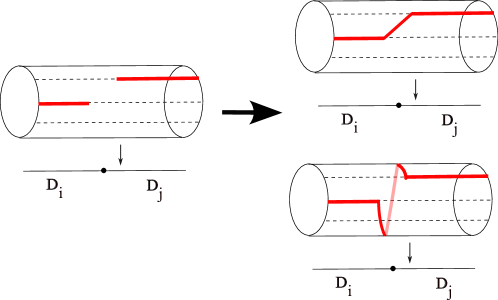
Figure 5. Extension of a partial section to a singular edge.

Since $\mathcal{E}=\mathbb{E}\Big{(}\sum_{i}ind_{s}(x_{i})\Big{)}=\sum_{i}\mathbb{E}(ind_{s}(x_{i})),$ it remains to compute the contribution $\mathbb{E}(ind_{s}(x))$ of each of the singular vertices.

Let us first give technical backgrounds of the computation. In a neighborhood of a singular vertex, a choice of a partial section over the domains $D_{i}$ that are incident to the vertex, amounts to a choice of a (possibly non-continuous) curve from the portrait which intersects each of the fibers exactly once, see Fig. 6.

Assume one goes in the ccw direction. At the points of discontinuity the curve makes $M$ jumps ”forwards”, that is, in the direction of the fiber, and $K$ jumps backwards.

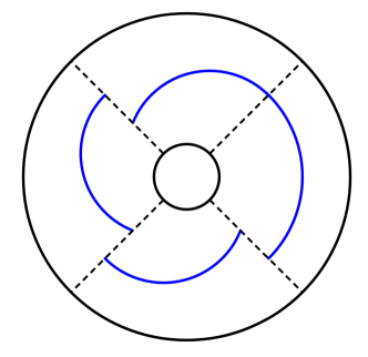
Figure 6. A choice of partial sections over the domains $D_{i}$ in a neighborhood of a singular vertex. Here $M=0,\ K=3$

A straightforward computation shows:

Lemma 5.

In the above notation, a choice of partial sections over $D_{i}$ contributes $\frac{K-M}{2}$.

Therefore $\mathbb{E}(ind_{s}(x))$ equals the average of $\frac{K-M}{2}$ over all possible choices of partial sections over the domains $D_{i}$ incident to $x$.

Lemma 6.

1. The contributions of a portrait and its image under a line symmetry sum up to zero.

2. If a portrait of a singular vertex has a line symmetry, the vertex contributes $0$.

3. Only essential singular vertices have non-zero expectation $\mathbb{E}(ind_{s}(x))$.

Proof.

(1) Indeed, line symmetry maps a partial section $s$ of an initial portrait to some partial sections of the symmetric image of the portrait. Besides, $K$ and $M$ exchange their roles. (2) follows from (1), since the numbers $\frac{K-M}{2}$ for two symmetric partial sections sum up to zero.

∎

Lemma 7.

For a right essential vertex of type $II$ (a right pleat),

$$\mathbb{E}(ind_{s}(x))=\frac{2}{(r+1)(r+3)}.$$

For a left essential vertex of type $II$ (a left pleat),

$$\mathbb{E}(ind_{s}(x))=\frac{-2}{(r+1)(r+3)}.$$

Proof.

Let’s prove the statement for a right pleat. The singular vertex has two incident domains $D_{i}$ and $D_{j}$, so the portrait is divided into two regions: a large sector and a small sector, see Fig. 7. Now, using Lemma 5, let us calculate the contribution of each of the partial sections. If we choose a red arc in the large sector and a red arc in the small sector, we get either two jumps down, as in case (a), or one jump down, as in cases (b) and (c). Their total contribution is $\frac{2}{2}+2\cdot\frac{1}{2}=2$. If we choose a blue arc in the small sector, we will have one downward and one upward jump, so the total contribution will be zero. Also, a choice of any blue arc in the large sector and any other arc in the small sector contributes zero. Since the total number of sections is $(r+1)(r+3)$, the averaging gives $\frac{2}{(r+1)(r+3)}$.

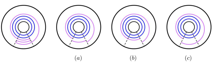
Figure 7. portrait of a pleat; choices of partial sections.

∎

Lemma 8.

For an essential vertex of type $I$,

$$\mathbb{E}(ind_{s}(x))=\frac{4({n}-{k})}{(n+k)(n+k+2)(n+k+4)}$$

Proof.

Figure 8. The four domains $D_{i}$ in a neighborhood of a type $I$ critical vertex.

The annulus is divided into four sectors, $a,b,c$ and $d$, see 8. the sectors come from four domains $D_{i}$ in a neighborhood of the vertex. By Lemma 5, we have to average $\frac{K-M}{2}$ over all choices of sheets in each of the sectors. A $4$-tuple of partial sections (over $a,b,c$ and $d$) yields two triples of partial sections, one triple is over the sectors $a,b,c$, and the other one is over $a,d,c$. Observe that the value $\frac{K-M}{2}$ behaves additively. Therefore we need to average $\frac{K-M}{2}$ for both of the triples and sum up. A computation (analogous to the previous lemma) shows that each triple contributes $\frac{2(n-k)}{(n+k)(n+k+1)(n+k+2)}$.

∎

Lemma 9.

For a right essential vertex of type $III$ ( a regular sheet intersects a fold),

$$\mathbb{E}(ind_{s}(x))=\frac{2}{(r+1)(r+3)}.$$

For a left essential vertex of type $III$,

$$\mathbb{E}(ind_{s}(x))=\frac{-2}{(r+1)(r+3)}.$$

Proof.

This can be proven by analogous computations. ∎

Theorem is proven for the case when all the domains $D_{i}$ are one-connected.

Non-one-connected domains $D_{i}$.

If there are domains that are not one-connected, the following trick helps. Let us enlarge $\mathcal{Q}$ by adding a disjoint with $\mathcal{Q}$ connected component. This new component is a topological sphere. Geometrically it looks like a thin ellipsoid (Hausdorff close to a line segment). On the one hand, a careful adding a number of such components makes all the $D_{i}$ one-connected, keeps the Euler number, and also keeps the portraits of already existing singular vertices. On the other hand, there arise new singular vertices of type $I$. They arise in pairs that differ on a line symmetry, therefore the corresponding weights are canceled.

∎

4. Examples of quasisections. Existence and non-existence

4.1. Elementary examples

A smooth section is a quasisection. Indeed, it can be viewed as an embedded closed manifold which projects bijectively to the base $B$. We remind the reader that existence of a continuous section is equivalent to triviality of the circle bundle.

Moreover, if a quasisection $\mathcal{Q}$ has no singularities (for instance, yields a covering of $B$), then $E\rightarrow B$ is also trivial.

One can fill $E$ with many mutually disjoint (topological) spheres and thus get a (disconnected) quasisection with type $I$ singular vertices only. Adding thin connecting tubes gives a connected embedded quasisection.

Example 1.

(Quasisections of the trivial bundle.) Let $\phi:Q\rightarrow B$ be a generic smooth map. Let $f:Q\rightarrow\mathbb{R}$ be a generic function such that $f(Q)\subset(0,1)$. Assume that the fibers of the bundle are consistently coordinatized by $\mathbb{R}/\mathbb{Z}$. Set $q(x)=(\phi(x),f(x))$. Adding $N$ disjoint continuous sections gives a quasisection. If $\pi\circ q$ is surjective, the number $N$ may be zero.

4.2. Quasisections with odd degree

Definition 3.

The degree $deg(\mathcal{Q})\in\mathbb{Z}_{2}$ (or $\mathbb{Z}$) of a quasisection is $deg(\pi\circ q)$.

Theorem 2.

1. If $Q$ is orientable, and $\mathcal{E}\neq 0$, then $deg(\mathcal{Q})=0\in\mathbb{Z}$.

2. If $Q$ is non-orientable, and $deg(\mathcal{Q})=1\in\mathbb{Z}_{2}$, then $\mathcal{E}$ is even.

3. For any even $\mathcal{E}$, there exists a non-orientable quasisection with $deg=1$.

Proof.

(1) and (2) follow from Gysin exact sequence.

An example for (3) is below. ∎

Example 2.

Assume $\mathcal{E}(E\rightarrow B)=2$. Take the base $B$ and a small disk $D\subset B$. The restriction of the bundle to $B\setminus Int(D)$ is trivial, so let us choose a continuous section $s$ over $B\setminus Int(D)$. One considers $s$ as a manifold $S$ with boundary lying in $E$. By construction, $\partial S\subset\pi^{-1}(\partial D)=\partial D\times S^{1}$. We may assume that $\partial S$ looks as in Fig. 9, left. Homotope $S$ as is depicted in Fig. 9, center. Next patch two discs to $\partial S$ (Fig. 9, right). One disc projects to $D$, and the other one embeds in $\partial D\times S^{1}$. We get a closed surface (one can check that it is the Klein bottle) which is piecewise smoothly mapped to $E$. A perturbation turners it to a smooth quasisection.

Our surgery acts in a neighborhood of $D$. Therefore the degree of $\pi\circ q$ equals $1$ since each of the points away from $D$ has a one-element preimage.

A quasisection for arbitrary even $\mathcal{E}=2k$ comes from an analogous construction for $k$ small disks $D_{i}\subset B$.

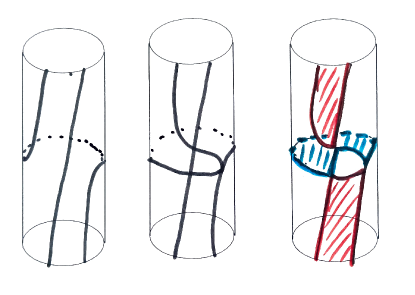
Figure 9. A quasisection with $deg=1$.

4.3. Pancake quasisections

A pancake quasisection is an embedding of a finite number of topological spheres in $E$ such that:

1. Each of the spheres projects with no pleats and with a unique circular fold.

2. The projections of the spheres have at most triple intersections.

The spheres are called pancakes since one imagines them to be very much flattened.

Assume we have a pancake quasisection, and $P_{1},P_{2}$ and $P_{3}$ are pancakes that intersect in the projection. The triple produces three singular vertices (the innermost intersection points) of type $I$. Each of them has weight either $1/6$, or $-1/6$, depending on the orientation of the triple $P_{1},P_{2},P_{3}$. Therefore the local formula reads as

$$\mathcal{E}(E\rightarrow B)=\frac{1}{2}(\hbox{ number of positively oriented triples of pancakes }-$$

$$\hbox{ number of negatively oriented triples}).$$

Figure 10. Two triples of pancakes, a negatively oriented (left) and a positively oriented (right).

Example 3.

The circle bundle over the sphere $S^{2}$ with $\mathcal{E}=2$ has a pancake quasisection with four pancakes. All the $12$ singular vertices are essential and have one and the same type $I$ with $n=2$, $k=0$.

Example 4.

(Two crossing pancakes, A)

Let $E\rightarrow B$ be a circle bundle with $\mathcal{E}=1$ over $B=S^{2}$. Let $U\subset B$ be a disk. The bundle has a continuous section $s_{1}$ over $U$, and a continuous section $s_{2}$ over $B\setminus U$. We think of these partial sections as of subsets of $E$. Take the $\varepsilon$-neighborhoods of $s_{1}$ and $s_{2}$ and their boundaries. We get two ”very flat” topological spheres (also called pancakes), but unlike the previous example, the pancakes are now crossing. The only essential vertices in this case are $4$ right essential vertices of type $III$ with $r=1$.

If $\mathcal{E}\geqslant 0$ is arbitrary, a similar construction gives $4\mathcal{E}$ right essential vertices of type $III$ with $r=1$

Example 5.

(Two crossing pancakes, B)

Let $E\rightarrow B$ be a trivial bundle over $B=S^{2}$. Take $n$ continuous disjoint sections and two crossing discs in $E$. Replacing the discs by their $\varepsilon$-neighborhoods gives two crossing pancakes. We arrive at a quasisection with $4$ singular vertices of type $III$, and $2$ singular vertices of type $I$.

Example 6.

(Curled pancake) Consider a trivial bundle over $S^{2}$. Let $\mathcal{Q}$ consist of $N$ disjoint continuous sections one curled pancake, see Fig. 11. There are two essential vertices of type $II$ and one of type $I$.

Figure 11. A curled pancake

5. Uniqueness of the local formula

Definition 4.

A local formula $\mathcal{F}$ computing the Euler number via singularities of quasisections is a triple of functions

$$\mathcal{F}_{ff}:(\mathbb{N}\cup\{0\})\times(\mathbb{N}\cup\{0\})\setminus\{0,0\}\rightarrow\mathbb{R},$$

$$\ \mathcal{F}_{p}:(\mathbb{N}\cup\{0\})\times\{L,R\}\rightarrow\mathbb{R},$$

$$\ \hbox{and}\ \ \mathcal{F}_{fs}:(\mathbb{N}\cup\{0\})\times\{L,R\}\rightarrow\mathbb{R}$$

such that for any circle bundle $E\rightarrow B$ and any quasisection $\mathcal{Q}$

$$\mathcal{E}(E\rightarrow B)=\sum_{I}\mathcal{F}_{ff}((n,k)(x_{i}))+\sum_{II}\mathcal{F}_{p}(n(x_{i}))+\sum_{III}\mathcal{F}_{fs}(n(x_{i})),$$

where $x_{i}$ ranges over essential vertices of $\mathcal{Q}$, and the numbers $n$ (and $k$ for the type $I$) are those defined in Section 2.2.

Theorem 3.

Any local formula coincides with that from Theorem 1. That is, we always have

$$\mathcal{F}_{ff}(n,k)\equiv\mathcal{W}_{ff}(n,k),\ \mathcal{F}_{p}(n)\equiv\mathcal{W}_{p}(n),\ \mathcal{F}_{fs}(n)\equiv\mathcal{W}_{fs}(n).$$

The proof is based on examples from Section 4 and goes by induction.

We apply local transformations to a quasisection: add pancakes or other connected components, create wrinkles, etc. These transformations keep the bundle, and therefore, the Euler number, but change the essential singular vertices and their weights in a controllable way.

Since local transformations keep the degree of the quasisection, we need two bases of induction, one for $deg=1$ and the other for $deg=0$.

So assume we are given some local formula $\mathcal{F}$.

Lemma 10.

(The antisymmetry property of $\mathcal{F}$)

1. $\mathcal{F}_{ff}(n,k)\equiv-\mathcal{F}_{ff}(k,n)$.

2. $\mathcal{F}_{p}(n,R)=-\mathcal{F}_{p}(n,L)$.

3. $\mathcal{F}_{fs}(n,R)\equiv-\mathcal{F}_{fs}(n,L)$.

Proof.

1. Take a quasisection $\mathcal{Q}$ and add two small disjoint pancakes, whose projections intersect at two points. We assume that the pancakes do not intersect $\mathcal{Q}$, and the projections of two new folds do not intersect the already existent singular curves. There arise two new singular vertices of type $I$, one with some parameters $(k,n)$, and the other with $(n,k)$. Since all other singular vertices and their weights persist, and $\mathcal{E}$ persists as well, the weights of the new singular vertices cancel each other.

2. Take a regular part of a quasisection $\mathcal{Q}$ and create a small wrinkle, that is, two pleats connected with folds. The parameters of the pleats are $r,L$ and $r,R$. Since all other singular vertices persist, and $\mathcal{E}$ persists as well, the weights of the two pleats cancel each other.

3. Take a regular point of $\mathcal{Q}$ and add a pancake that crosses $\mathcal{Q}$ in the small neighborhood of this point. There appear two new singular vertices of type $III$, one is $(n,R)$, and the other is $(n,L)$. By similar reasons their weights cancel each other.

∎

Lemma 11.

(Induction step for Type $I$)

$\mathcal{F}_{ff}(n,k)$ is uniquely determined by $\mathcal{F}_{ff}(1,0),\mathcal{F}_{ff}(2,0),$ and $\mathcal{F}_{ff}(3,0)$.

Proof.

We shall prove that $\mathcal{F}_{ff}(n,k)$ is a linear combination of $\mathcal{F}_{ff}(1,0),\mathcal{F}_{ff}(2,0),$ and $\mathcal{F}_{ff}(3,0)$ with coefficients depending on $n$ and $k$. The proof goes by induction. Consider a quasisection $\mathcal{Q}$ of the trivial bundle over $S^{2}$ which is a disjoint union of three disjoint pancakes $P_{1},P_{2},P_{3}$ (whose projections have a triple intersection), and $m\geqslant 2$ disjoint continuous sections, called simple sheets. The quasisection has $6$ singular vertices, all of them of type $I$ . Assume that there are $a$ simple sheets between pancakes $P_{1}$ and $P_{2}$, $b$ simple sheets lying between $P_{2}$ and $P_{3}$, and $c=m-a-b$ simple sheets between $P_{3}$ and $P_{1}$.

We shall use the local formula:

$$\mathcal{F}_{ff}(a+b+2,c)+\mathcal{F}_{ff}(b+c+2,a)+\mathcal{F}_{ff}(c+a+2,b)+$$

$$+\mathcal{F}_{ff}(a+b,c)+\mathcal{F}_{ff}(b+c,a)+\mathcal{F}_{ff}(c+a,b)=0,$$

and also Lemma 10:

$$\mathcal{F}_{ff}(s,m+2-s)=-\mathcal{F}_{ff}(m+2-s,s).$$

Assuming that $\mathcal{F}_{ff}(a+b,c)+\mathcal{F}_{ff}(b+c,a)+\mathcal{F}_{ff}(c+a,b)$ for all $a+b+c=m$ is known, prove that $\mathcal{F}_{ff}(n,k)$ is uniquely defined for $n+k=m+2$.

For a fixed $m$, we arrive at a system of linear equations with unknowns
$\mathcal{F}_{ff}(m+2-a,a),\ \ a=0,1,...,m+2$. To prove the uniqueness of its solution, let us consider the corresponding homogenous system. It reads as

$$\left\{\begin{array}[]{ll}g(a)+g(b)+g(c)=0,&\hbox{ for $a+b+c=m$;}\\ g(a)+g(m+2-a)=0,&\hbox{for $0\leqslant a\leqslant m+2$.}\end{array}\right.$$

Since $g(0)+g(0)+g(m)=0,$ and $g(2)+g(n)=0$, we get $g(2)=2g(0)$. Since $g(1)+g(1)+g(n-2)=g(0)+g(2)+g(n-2)$, then $2g(1)=g(0)+g(2)$, so $g(1)=\frac{3}{2}g(0)$. Proceeding in a similar way, we get $g(k)=(\frac{k}{2}+1)g(0)$ for all $k$. The second equation gives $0=g(0)+g(m+2)=g(0)(2+\frac{n+2}{2})$, which implies $g(0)=0$ and completes the proof.
∎

Lemma 12.

(Induction step for Type $II$)

$$\mathcal{F}_{p}(n+2,R)=\mathcal{F}_{p}(n,R)-\mathcal{F}_{ff}(n+1,0)+\mathcal{F}_{ff}(n,1)$$

Proof.

Assume a quasisection has a right pleat with $n$ simple circles in the portrait. Add a small pancake right over the pleat whose projection embraces the projection of the pleat. The pleat turns to a pleat with $n+2$ simple circles in the portrait. Besides, there arise two type $I$ singular vertices. Since the Euler class persists, the difference of two local formulae is zero. ∎

Lemma 13.

(Type $III$ reduces to Type $I$)

$$\mathcal{F}_{fs}(n+1,R)=1/2\mathcal{F}_{ff}(n,0).$$

Proof.

The local formula for Example 5 reads as $2\mathcal{F}_{ff}(0,n)+4\mathcal{F}_{fs}(n+1,L)=0$. ∎

Lemma 14.

(The base of induction, degree $0$)

1. $\mathcal{F}_{ff}(2,0)=\mathcal{W}_{ff}(2,0)=1/6$.

2. $\mathcal{F}_{fs}(1,R)=\mathcal{W}_{fs}(1,R)=1/4$.

3. $\mathcal{F}_{p}(1,R)=\mathcal{W}_{p}(1,R)=1/4$.

Proof.

(1) follows from Example 3.

(2) follows from Example 4.

(3) Take the Boy surface [18], place it in the total space of the trivial bundle $S^{2}\times S^{1}\rightarrow S^{2}$, and add two continuous sections, disjoint from the Boy surface. We get a quasisection with degree $2$. The local formula $\mathcal{F}$ reads as

$$0=3\mathcal{F}_{p}(3,R)+3\mathcal{F}_{fs}(3,R)-3\mathcal{F}_{ff}(2,0).$$

Applying Lemma 12, (1) and (2), one gets

$$\mathcal{F}_{p}(1,R)=1/4=\mathcal{W}_{p}(1,R).$$

∎

Lemma 15.

$$\mathcal{F}_{ff}(3,0)=\frac{3}{7}\mathcal{F}_{ff}(1,0),\ \ \mathcal{F}_{ff}(2,1)=\frac{1}{7}\mathcal{F}_{ff}(1,0).$$

Proof.

Let us prove that

$$\begin{cases}2\mathcal{F}_{ff}(3,0)+\mathcal{F}_{ff}(0,1)+\mathcal{F}_{ff}(2,1)=0\\ \mathcal{F}_{ff}(0,1)+\mathcal{F}_{ff}(3,0)+4\mathcal{F}_{ff}(2,1)=0\\ \end{cases}$$

Take a trivial bundle over $S^{2}$ with one continuous section and three pancakes as in Fig. 10. The local formula gives the first equation.

For the second equation let us take a trivial bundle over $S^{2}$ with one curled pancake and one small pancake placed over one of the pleats.The local formula gives: $\mathcal{F}_{p}(2,L)+\mathcal{F}_{p}(4,L)+\mathcal{F}_{ff}(0,1)+\mathcal{F}_{ff}(2,1)+\mathcal{F}_{ff}(2,1)=0$. Application of the antisymmetry property and Lemma 12 complete the proof. ∎

Lemma 16.

(The base of induction, degree $1$)

1. $\mathcal{F}_{ff}(1,0)=\mathcal{W}_{ff}(1,0)=4/15$.

2. $\mathcal{F}_{p}(0,R)=\mathcal{W}_{p}(0,R)=2/3$.

3. $\mathcal{F}_{fs}(0,R)=\mathcal{W}_{fs}(0,R)=2/3$.

Proof.

Let us take the Boy surface, place it in the total space of the trivial bundle $S^{2}\times S^{1}\rightarrow S^{2}$, and add a continuous section. The union of the Boy surface and the continuous section is a quasisection with degree $1$. Application of the local formula $\mathcal{F}$ and Lemma 11 give:

$$0=3\mathcal{F}_{p}(2,R)+3\mathcal{F}_{fs}(2,R)-3\mathcal{F}_{ff}(1,0)=$$

$$=3(\mathcal{F}_{p}(0,R)-\mathcal{F}_{ff}(1,0)+\mathcal{F}_{ff}(0,1))+3/2\mathcal{F}_{ff}(1,0)-3\mathcal{F}_{ff}(1,0)=$$

$$=3\mathcal{F}_{p}(0,R)-3/2\mathcal{F}_{ff}(1,0).$$

We get a homogeneous linear equation which includes unknowns $\mathcal{F}_{p}(0,R)$ and $\mathcal{F}_{ff}(1,0)$.

Next, we take the quasisection from Example 2, where $deg=1$, and the Euler number is $2$. Applying the local formula $\mathcal{F}$ together with the above lemmata, we get

$$2=\lambda\mathcal{F}_{p}(0,R)+\mu\mathcal{F}_{ff}(1,0)$$

for some coefficients $\lambda$ and $\mu$. Thus we obtain a system of linear equations which has a unique solution.

∎

Theorem 3 is proven.

References

- [1] V. I. Arnold, S. Gusein-Zade, A. Varchenko, Singularities of Differentiable Maps vol. I, Monographs Math. 82, Birkhäuser, (1985).
- [2] S. Chern, Circle bundles, Lect. Notes Math. 597 (1977), 114-131.
- [3] A. Fomenko, D. Fuchs, Homotopical Topology, Springer, 2016
- [4] Y. M. Eliashberg, Ob osobennostjah tipa skladki, Izv. Akad. Nauk SSSR Ser. Mat. 34:5 (1970), 1110-1126. Translated as On singularities of folding type in Math. USSR Izv. 4:5 (1970), 1119-1134.
- [5] T. Fukui, M. Hasegawa, Height functions on Whitney umbrellas, RIMS Kôkyûroku Bessatsu B38, 153-168 (2013).
- [6] A. Haefliger, Quelques Remarques sur les Applications Différentiables d’une Surface sur le Plan. Ann. Inst. Fourier, Grenoble10 (1960), 47-60.
- [7] K. Igusa, Combinatorial Miller-Morita-Mumford classes and Witten cycles, Algebr. Geom. Topol., 4, 2004, 473–520.
- [8] M. Kazarian, The Chern-Euler number of circle bundle via singularity theory, Math. Scand., 82:2 (1998), 207-236.
- [9] J.H. Milnor, J.D. Stasheff, Characteristic Classes, Annals of Mathematics Studies 76. Princeton University Press, (1974) Princeton.
- [10] N. Mnëv, Minimal triangulations of circle bundles, circular permutations, and the binary Chern cocycle, Zap. Nauch. Semin. POMI, 481, 2019, 87–107.
- [11] N. Mnëv, G. Sharygin, On local combinatorial formulas for Chern classes of a triangulated circle bundle, Zap. Nauch. Semin. POMI, 448, 2016, 201–235.
- [12] J. R. Quine, A global theorem for singularities, Trans. Amer. Math. Soc., 236 (1978), 307-314.
- [13] T. Yamamoto, Number of singularities of stable maps on surfaces, Pacific J. Math., Vol. 280, No. 2, 2016
- [14] R. Thom, Les singularites des applications differentiables, Ann. Inst. Fourier (Grenoble) 6 (1955/56) 43-87.
- [15] H. Whitney, On regular closed curves in the plane, Compositio Math. 4 (1937) 276-284.
- [16] R. Pignoni,Projections of surfaces with a connected fold curve, Topology and its Applications 49 (1993) 55-74.
- [17] S. Reshetova, Around local combinatorial formulae for -bundles, unpublished, https://dspace.spbu.ru/bitstream/11701/39921/2/diplom_Reshetova.pdf
- [18] A model of Boy’s surface in Constructive Solid Geometry, https://www.math.univ-toulouse.fr/~cheritat/boy-surface/index.html