Engineering propagating cat states with driving-assisted cavity QED

Abstract

We propose a method for generating optical cat states in propagating pulses based on cavity quantum electrodynamics (QED). This scheme uses multiple four-level systems (4LSs) inside an optical cavity as an emitter. Time-modulating driving stimulates the emitter to produce a superposition of coherent states entangled with the 4LSs. The postselection of an appropriate state of the 4LSs leads to a multicomponent cat state in a propagating pulse. Taking atomic decay and cavity loss into account, we optimize the cavity external loss rate to maximize the fidelity. We find that its optimum value is formulated similarly to that of other generation methods for propagating states, which suggests a universal property of cavity-QED systems interacting with fields outside the cavity.

I Introduction

Propagating nonclassical light is one of the promising systems for quantum information processing. The propagating optical state has several advantages: high scalability using time- or frequency-domain-multiplexing methods [1, 2, 3] and high feasibility for long-distance quantum communication [4]. To generate nonclassical light with “Wigner-negativity” [5], two exemplary methods are known. The first is the use of quantum entanglement and measurements of light [6, 7]. The second is based on the nonlinear interaction between matter and light.

While the former method requires photon number counting to generate complex optical states, the latter does not require such measurements. Notably, a nonlinear system inside an optical cavity, which is treated in cavity quantum electrodynamics (QED), is a promising system for generating nonclassical lights because it can harness the strong interaction between matter and light. Generating nonclassical light with cavity-QED systems has been studied on both the theoretical and experimental sides. For example, a single photon has been generated by various systems, e.g., neutral atoms [8, 9], ions [10, 11], defects in solids [12, 13], and generating $N$-photon states has been proposed [14]. These discrete-variable (DV) states are generated by driving a nonlinear system inside the cavity. On the other hand, continuous-variable (CV) states, such as Schrödinger cat states (superpositions of coherent states) and Gottesman-Kitaev-Preskill states [15], can be generated by reflecting an optical state off the cavity QED systems [16, 17, 18]. However, in these schemes, (nonclassical) seed light must repeatedly pass through circulators and reflect off the cavity, which introduces additional losses, pulse distortions, and complications of the setup, and thus it will be difficult to generate desired states with high fidelity.

In this paper, we propose a protocol for generating cat states by driving four-level systems (4LSs) inside a cavity. Our protocol generates entanglement between the 4LSs and a superposition of coherent states in a propagating pulse output from the cavity. If we use a single 4LS and measure it after driving, we can generate a superposition of two coherent states, $\ket{\alpha}\pm\ket{-\alpha}$, namely, a Schrödinger cat state. Moreover, by driving and measuring two 4LSs and postselecting the measurement result, we can generate a four-component cat state $\ket{\beta}+\ket{-\beta}+\ket{i\beta}+\ket{-i\beta}$. Our protocol can tailor the temporal pulse shape by controlling driving pulses, similar to the conventional driving methods for DV states [19, 14, 20]. Notably, this does not require circulators or repeating reflection, and thus prevents additional optical loss, unlike conventional reflecting methods for CV states. We also discuss the requirement of the pulse length for high-fidelity generation. The length limit we find is consistent with that of the other driving methods. Moreover, taking atomic decay and cavity loss into account, we optimize the cavity external loss rate to maximize the fidelity. We find that its optimum value is formulated similarly to that of the other generation methods for propagating states. These results suggest a universal property of cavity-QED systems interacting with fields outside the cavity.

II Generating Schrödinger cat states

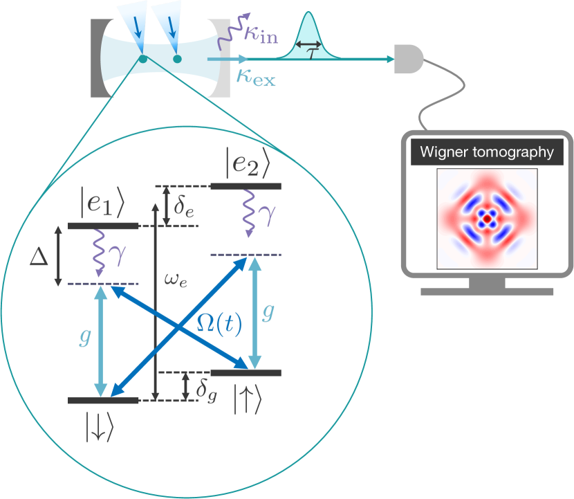
Figure 1: Schematic of the proposed protocol.

We consider a 4LS with two ground and excited states inside a one-sided optical cavity, where two optical transitions couple with a single cavity mode $\hat{c}$ and the two other diagonal transitions are driven by $\sigma_{+}$- and $\sigma_{-}$- polarized laser fields (see Fig. 1). The Hamiltonian of the 4LS in the rotating-wave approximation and a proper rotating frame is given as $(\hbar=1)$

$$\hat{H}_{\text{4LS}}= \ab(\Delta-\frac{\delta_{e}}{2})\outerproduct{e_{1}}{e_{1}}+\ab(\Delta+\frac{\delta_{e}}{2}-\delta_{g})\outerproduct{e_{2}}{e_{2}}$$ (1)

$$+\Big{[}\Omega(t)\ab(\outerproduct{e_{2}}{\downarrow}+\outerproduct{e_{1}}{\uparrow})$$

$$\quad\quad+g(\outerproduct{e_{1}}{\downarrow}+\outerproduct{e_{2}}{\uparrow})\hat{c}+\text{H.c.}\Big{]}.$$

Here, $\delta_{g}\,(\delta_{e})$ is the difference frequency between the ground spin (excited) states, $\Delta=\omega_{e}-\omega_{c}$ is the detuning between the optical transition frequency and the cavity frequency, and $g$ is the cavity coupling strength. We have assumed that the frequency of the laser field that couples $\ket{\downarrow}\text{-}\ket{e_{2}}\,(\ket{\uparrow}\text{-}\ket{e_{1}})$ is $\omega_{c}+\delta_{g}\,(\omega_{c}-\delta_{g})$. In the following, we also assume a sufficiently large $\Delta$ such that we can neglect the difference between the energy of spin (excited) states and adiabatically eliminate the excited states, which allows us to obtain a simplified effective Hamiltonian given as [21, 22](see Appendix A)

$$\hat{H}^{\text{eff}}_{\text{4LS}}=\omega_{0}\hat{c}^{\dagger}\hat{c}+\hat{\sigma}_{x}(\lambda^{\ast}(t)\hat{c}+\lambda(t)\hat{c}^{\dagger}),$$ (2)

where we define $\hat{\sigma}_{x}=\outerproduct{\uparrow}{\downarrow}+\outerproduct{\downarrow}{\uparrow}$ and the parameters are given as follows:

$$\omega_{0}=-\frac{g^{2}}{\Delta},\quad\lambda(t)=-\frac{g\Omega(t)}{\Delta}.$$ (3)

Note that such a simplified model is originally proposed in Ref. [21] for mimicking the Dicke model, and has been demonstrated by using ${}^{87}\text{Rb}$ atoms inside an optical cavity [23].

To present the essence of our protocol, we first neglect the atomic decay, which is discussed later. We assume that the cavity mode couples a desired output mode at rate $\kappa_{\text{ex}}$ and an unwanted mode at rate $\kappa_{\text{in}}$, which corresponds to internal loss and scattering at the mirrors. We use the input-output theory [24] to formulate the dynamics. We also assume that the 4LS is initially in the spin manifold $\{\ket{\downarrow},\ket{\uparrow}\}$, and both of the cavity and output modes are in vacuum states. From the commutation relation $[\hat{\sigma}_{x},\hat{H}^{\text{eff}}_{\text{4LS}}]=0$, $\hat{\sigma}_{x}(t)$ is time-independent and can be denoted simply by $\hat{\sigma}_{x}(0)$. For $\hat{c}(t)$, we obtain

$$\dot{\hat{c}}=-(i\omega_{0}+\kappa)\hat{c}-i\lambda(t)\hat{\sigma}_{x}(0),$$ (4)

where the dot denotes the time derivative and we have defined $\kappa=\kappa_{\text{ex}}+\kappa_{\text{in}}$. Here, we choose the Rabi frequency $\Omega(t)=-\lambda(t)\Delta/g$ with

$$\lambda(t)=\frac{i\alpha}{\sqrt{2\kappa_{\text{ex}}}}\ab[\dot{v}(t)+(i\omega_{0}+\kappa)v(t)],$$ (5)

where $\alpha$ is a complex number and $v(t)$ is an envelope function satisfying $\int_{0}^{\infty}\differential{t}|v(t)|^{2}=1$ and $v(0)=\lim_{t\to\infty}v(t)=0$. This choice gives the cavity mode as

$$\hat{c}(t)=\frac{v(t)}{\sqrt{2\kappa_{\text{ex}}}}\alpha\hat{\sigma}_{x}(0)$$ (6)

and we find that the desired output mode is given as $\hat{a}_{\text{out}}(t)=v(t)\alpha\hat{\sigma}_{x}(0)$ by using the input-output relation $\hat{a}_{\text{out}}(t)=\sqrt{2\kappa_{\text{ex}}}\hat{c}(t)$. Thus, after driving the 4LS, the desired output mode becomes a coherent state with a temporal mode $v(t)$ whose amplitude depends on the initial spin state of the 4LS. When we prepare the initial spin-cavity state as $\ket{0}_{c}(b_{0}\ket{0}+b_{1}\ket{1})$ and assume $\kappa_{\text{in}}=0$, we can generate the hybrid entangled state $\ket{0}_{c}(b_{0}\ket{0}\ket{\alpha;v}_{\text{ex}}+b_{1}\ket{1}\ket{-\alpha;v}_{\text{ex}})$. Here, $\ket{j}=(\ket{\downarrow}+(-1)^{j}\ket{\uparrow})/\sqrt{2}$, $\ket{n}_{c}$ is the $n$-photon state in the cavity mode, and $\ket{\alpha;v}_{\text{ex}}$ is a coherent state with a temporal mode $v(t)$ in the desired output mode. Thus, if we prepare the initial state as $\ket{\downarrow}$ and observe $\ket{\downarrow}\,(\ket{\uparrow})$ after driving, we obtain an even (odd) cat state $(\ket{\alpha}+\ket{-\alpha})/\mathcal{N}_{+}\,[(\ket{\alpha}-\ket{-\alpha})/\mathcal{N}_{-}]$ where $\mathcal{N}_{\pm}=\sqrt{2(1\pm e^{-2|\alpha|^{2}})}$ is a normalized factor.

Now, we investigate the performance of our protocol including the effect of cavity loss and atomic decay. The density operator of the total system, which includes the 4LS, the cavity mode, and the propagating light with the temporal mode $v(t)$, evolves according to a master equation

$$\odv{\hat{\rho}}{t}=-i[\hat{H},\hat{\rho}]+\sum_{m}\ab(\hat{L}_{m}\hat{\rho}\hat{L}_{m}^{\dagger}-\frac{1}{2}\{\hat{L}_{m}^{\dagger}\hat{L}_{m},\hat{\rho}\}),$$ (7)

where the Hamiltonian and the Lindblad operators are given as follows:

$$\begin{gathered}\hat{H}(t)=\hat{H}_{\text{4LS}}(t)+\frac{i}{2}\sqrt{2\kappa_{\text{ex}}}\ab[g_{v}^{\ast}(t)\hat{c}^{\dagger}\hat{a}_{v}-g_{v}(t)\hat{c}\hat{a}_{v}^{\dagger}],\\ \hat{L}_{0}(t)=\sqrt{2\kappa_{\text{ex}}}\hat{c}+g_{v}^{\ast}(t)\hat{a}_{v}(t),\quad\hat{L}_{1}=\sqrt{2\kappa_{\text{in}}}\hat{c},\\ \hat{L}_{2}=\sqrt{2r_{1}\gamma}\outerproduct{\downarrow}{e_{1}},\quad\hat{L}_{3}=\sqrt{2(1-r_{1})\gamma}\outerproduct{\uparrow}{e_{1}},\\ \hat{L}_{4}=\sqrt{2r_{2}\gamma}\outerproduct{\uparrow}{e_{2}},\quad\hat{L}_{5}=\sqrt{2(1-r_{2})\gamma}\outerproduct{\downarrow}{e_{2}},\end{gathered}$$ (8)

where $r_{1}(r_{2})$ is a branting ratio. Following the virtual-cavity method proposed in Refs. [25, 26], the master equation (7) describes a Gedanken-experiment where we put another one-sided cavity with complex input coupling

$$g_{v}(t)=-\frac{v^{\ast}(t)}{\sqrt{\int_{0}^{t}\differential{t^{\prime}}|v(t^{\prime})|^{2}}}$$ (9)

that completely absorbs a propagating state with a temporal mode $v(t)$. The operator $\hat{a}_{v}$ is an annihilation operator of the virtual cavity. As mentioned above, we focus on the regime where the detuning is sufficiently large and excited states can be adiabatically eliminated. Thus, we can reduce the master equation (7) to the effective one (see Appendix A). We numerically solve the effective master equation, unless stated otherwise. Assuming the initial state as $\ket{0}_{c}\ket{\downarrow}\ket{0}_{v}$, we evaluate the fidelity $\innerproduct{[}{[}3]{\text{cat}}{\hat{\rho}}{\text{cat}}$, where the Schrödinger-cat entangled state $\ket{\text{cat}}$ is defined as

$$\ket{\text{cat}}=\ket{0}_{c}\frac{\ket{0}\ket{\alpha}_{v}+\ket{1}\ket{-\alpha}_{v}}{\sqrt{2}}.$$ (10)

Here, $\ket{\alpha}_{v}$ is a coherent state in the virtual cavity mode. In the following, we set $\alpha=2$ and the temporal mode function as the Gaussian function

$$v(t)=\sqrt{\frac{1}{\sqrt{\pi}\tau}}\exp\ab[-\frac{1}{2}\ab(\frac{t-t_{0}}{\tau})^{2}],$$ (11)

where $t_{0}$ is a sufficiently large value such that $v(0)\to 0$.

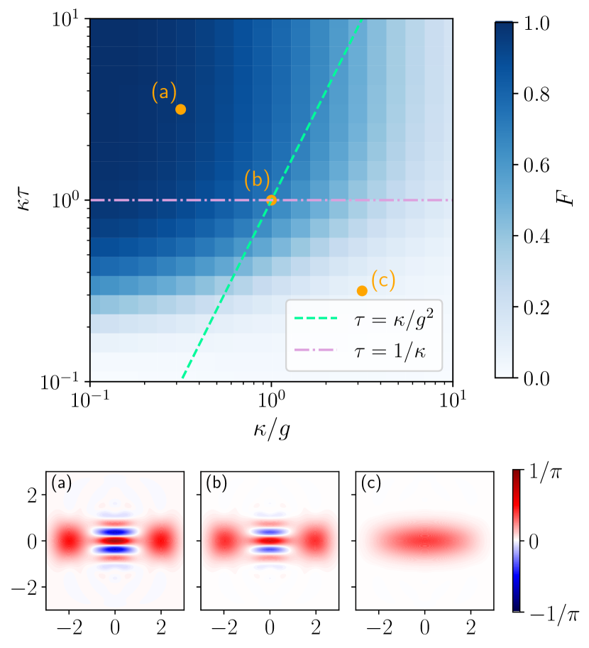
Figure 2: Fidelity for the Schrödinger-cat entangled state as a function of $\kappa/g$ and $\kappa\tau$ and Wigner functions of the output field. The cavity QED parameters are set as $(\Delta,g,\kappa_{\text{in}})=(1000,10,0.01)\gamma$ and $r_{1}=r_{2}=0.5$. We plot the Wigner functions of the output field after postselecting the case where the 4LS in $\ket{\downarrow}$ with the parameters that the dots show.

We first investigate how short a pulse can be generated by the system. Regarding the timescale of energy exchange between the atomic system and the output field through the cavity mode, there are two characteristic frequencies: $g$ and $\kappa$. When $g\gg\kappa$, the exchange speed between the atomic system and the cavity mode is faster than that between the cavity mode and the output field, and therefore the cavity decay rate $\kappa$ limits the total exchange speed. When $\kappa\gg g$, the exchange speed between the cavity mode and the output field is faster and the total exchange speed is determined by the Purcell-effect-enhanced atomic dipole decay rate into the cavity mode $g^{2}/\kappa$ [27]. Thus, we predict that we have to set $\tau\gg\tau_{c}\coloneqq\max(1/\kappa,\kappa/g^{2})$ for high-fidelity generation. This requirement is also valid for single-photon storage and generation [28, 20]. Figure 2 shows the fidelity as a function of $\kappa\tau$ and $\kappa/g$. We find that the requirement $\tau\gg\tau_{c}$ is also valid for generating the Schrödinger-cat entangled state, as expected.

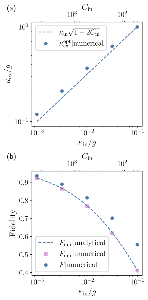
Figure 3: Optimized $\kappa_{\text{ex}}$ for generating the Schrödinger-cat entangled state. The parameters other than $\kappa_{\text{in}}$ are the same as Fig. 2 and we set $\tau=5\tau_{c}$. (a) Numerically optimized $\kappa_{\text{ex}}$ to maximize the fidelity $F$. (b) Numerical results for $F$ and $F_{\text{min}}$ with numerically optimized $\kappa_{\text{ex}}$. The dashed line represents $F_{\text{min}}$ given in Eq. (14) with $\kappa_{\text{ex}}=\kappa_{\text{in}}\sqrt{1+2C_{\text{in}}}$.

Assuming that $\tau$ satisfies the requirements, the fidelity will reach a value determined by the performance of the cavity-QED system and the amplitude of the coherent state. The performance of a cavity-QED system with an output field has been described by two parameters: the cooperativity $C=g^{2}/(2\kappa\gamma)$ and the escape efficiency $\kappa_{\text{ex}}/\kappa$ [29, 18]. An increase in both parameters is preferable. However, there is a trade-off relation between them with respect to $\kappa_{\text{ex}}$, and thus we have to carefully tune $\kappa_{\text{ex}}$ to maximize the fidelity, which can be achieved by tuning the reflectance of the mirror. To analytically analyze this tradeoff, we first decompose the generated state $\hat{\rho}$ as $\hat{\rho}=\outerproduct{\Psi}{\Psi}+\hat{\rho}_{\text{jumps}}$ with $\outerproduct{\Psi}{\Psi}$ representing an unnormalized state where no atomic decay and cavity loss occur and $\hat{\rho}_{\text{jumps}}$ representing an unnormalized state where one or more quantum jumps occur. When preparing the initial state as $\sum_{j}b_{j}\ket{0}_{c}\ket{j}\ket{\text{vac}}$, where $\ket{\text{vac}}$ denotes a vacuum state of all output modes, and assuming $\omega_{0}/\kappa=-g^{2}/(\kappa\Delta)\simeq 0$, we can derive the unnormalized state with no quantum jumps as (see Appendix C)

$$\ket{\Psi}=e^{-(1/P-1)|\alpha|^{2}/2}\sum_{j}b_{j}\ket{0}_{c}\ket{j}\ket{(-1)^{j}\alpha;v}_{\text{ex}},$$ (12)

where we have defined

$$P=\frac{\kappa_{\text{ex}}}{\kappa}\frac{2C}{1+2C}.$$ (13)

Thus, the fidelity with the ideal state $\ket{\psi_{\text{id}}}=\sum_{j}b_{j}\ket{0}_{c}\ket{j}\ket{(-1)^{j}\alpha;v}_{\text{ex}}$ is lower bounded as follows:

$$F=\innerproduct{[}{[}3]{\psi_{\text{id}}}{\hat{\rho}}{\psi_{\text{id}}}\geq e^{-(1/P-1)|\alpha|^{2}}(\eqqcolon F_{\text{min}}),$$ (14)

and we can maximize $F_{\text{min}}$ with $\kappa_{\text{ex}}=\kappa_{\text{in}}\sqrt{1+2C_{\text{in}}}$. Here, $C_{\text{in}}=g^{2}/(2\kappa_{\text{in}}\gamma)$ is known as the internal cooperativity, which is a performance measure of a cavity-QED system after optimizing $\kappa_{\text{ex}}$ [29, 18]. We numerically calculate $\hat{\rho},\ket{\Psi}$, and optimize $\kappa_{\text{ex}}$ for each $\kappa_{\text{in}}$ to maximize $F$, and then plot $F_{\text{min}}$ and $F$ with numerically optimized $\kappa_{\text{ex}}$ (see Fig. 3). Here, we calculate $\ket{\Psi}$ by solving the effective non-Hermitian Schrödinger equation (see Appendix A). As shown in Fig. 3, the numerically optimized $\kappa_{\text{ex}}$ is close to $\kappa_{\text{in}}\sqrt{1+2C_{\text{in}}}$. Considering $C_{\text{in}}\gg 1$ for high fidelity, we can suggest that the optimal $\kappa_{\text{ex}}$ will be proportional to $g\sqrt{\kappa_{\text{in}}/\gamma}$. Note that $P$ is the performance measure of generating single photons in a driving manner and cat states by a reflection manner with a single atom inside a cavity [29, 17]. Thus, these previous results and the result from this study imply that $P$ is a universal performance measure for generating propagating light with a single atom inside a cavity.

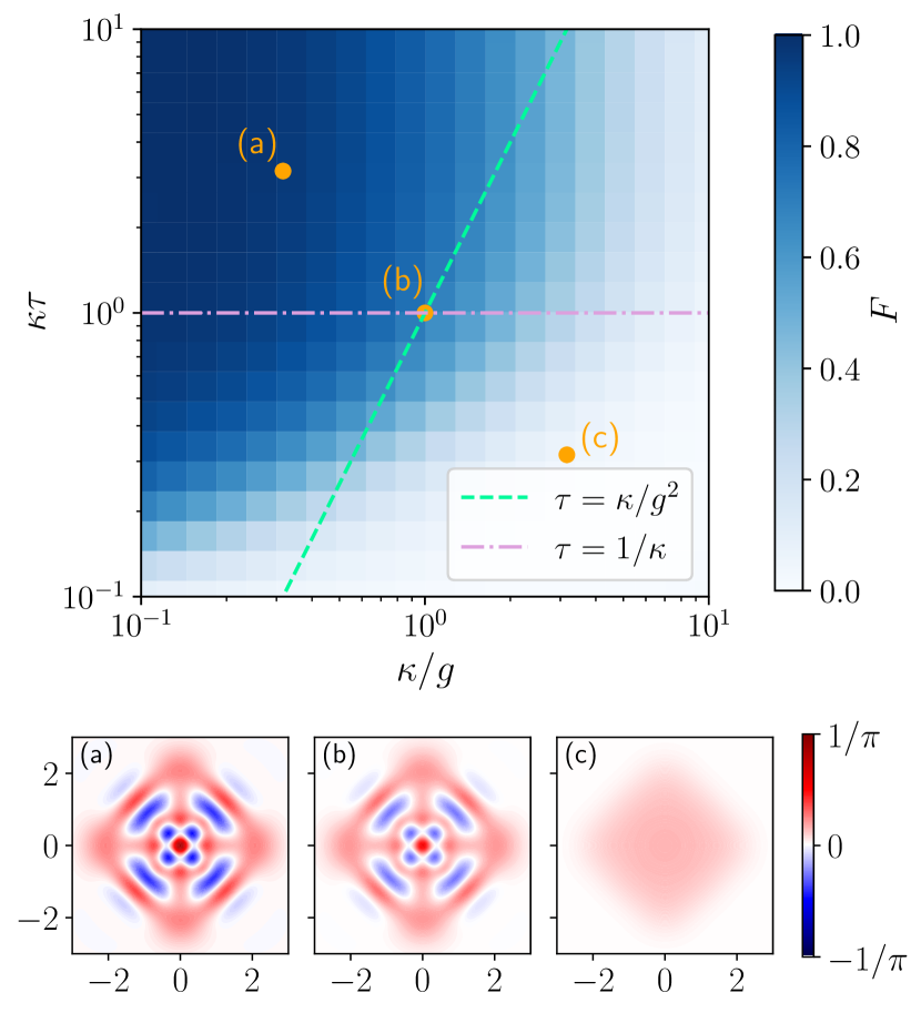
Figure 4: Fidelity for the four-component cat state as a function of $\kappa/g$ and $\kappa\tau$ and Wigner functions of the output field. The parameters are the same as Fig. 2. We plot the Wigner functions of the output field after postselecting the case where the 4LSs in $\ket{\downarrow}_{1}\ket{\downarrow}_{2}$ with the parameters that the dots show.

III Generating four-component cat states

Adding another 4LS inside the cavity allows for generating more complex entangled states. We assume that we can individually apply laser fields to the 4LS $i\,(i=1,2)$ with the time-dependent Rabi frequency $\Omega_{i}(t)=-\lambda_{i}(t)\Delta/g$, where

$$\lambda_{i}(t)=\frac{i\alpha_{i}}{\sqrt{2\kappa_{\text{ex}}}}\ab[\dot{v}(t)+(i2\omega_{0}+\kappa)v(t)].$$ (15)

When the two 4LSs are initially in $\ket{\downarrow}_{1}\ket{\downarrow}_{2}$ and we set $\alpha_{1}=\beta e^{i\pi/4}/\sqrt{2}$ and $\alpha_{2}=\beta e^{-i\pi/4}/\sqrt{2}$, we can generate the entangled state $\sum_{jl}\ket{j}_{1}\ket{l_{x}}_{2}\ket{(-1)^{j}i^{j+l}\beta;v}/2$ (see Appendix B). After postselecting the case where the 4LSs are in the state $\ket{\downarrow}_{1}\ket{\downarrow}_{2}$, the propagating light becomes a four-component cat state $(\ket{\beta;v}+\ket{-\beta;v}+\ket{i\beta;v}+\ket{-i\beta;v})/N_{\beta}$, where $N_{\beta}$ is a normalized factor. This state has various applications in optical quantum computation and quantum communication [30, 31, 32, 33]. Notably, no study has succeeded in generating such a state in the optical domain, although several theoretical studies have proposed generation methods [34, 35, 36].

We discuss the pulse length of the output light and optimization of $\kappa_{\text{ex}}$ as in the case of the Schrödinger-cat entangled state generation (Sec. II). We numerically solve the dynamics and evaluate the fidelity

$$F=\frac{\bra{\text{four-cat}}\innerproduct{[}{[}3]{\downarrow\downarrow}{\hat{\rho}}{\downarrow\downarrow}\ket{\text{four-cat}}}{\Tr[\innerproduct{[}{[}3]{\downarrow\downarrow}{\hat{\rho}}{\downarrow\downarrow}]}$$ (16)

where

$$\ket{\text{four-cat}}=\ket{0}_{c}\frac{\ket{\beta}_{v}+\ket{-\beta}_{v}+\ket{i\beta}_{v}+\ket{-i\beta}_{v}}{N_{\beta}},$$ (17)

and we set $\beta=2$. For the pulse length, the simulation result in Fig. 4 shows that the same requirement: $\tau\gg\tau_{c}\coloneqq\max(1/\kappa,\kappa/g^{2})$ is required. For optimizing $\kappa_{\text{ex}}$, we find that the numerically optimized $\kappa_{\text{ex}}$ is close to $\kappa_{\text{in}}\sqrt{1+3C_{\text{in}}}$ (see Fig. 5). Thus, considering $C_{\text{in}}\gg 1$ for high fidelity, the optimal $\kappa_{\text{ex}}$ will be proportional to $g\sqrt{\kappa_{\text{in}}/\gamma}$, which is the same attitude in the case of the Schrödinger-cat entangled state. Such a universal attitude is interesting and investigating its physical origin is left for future work.

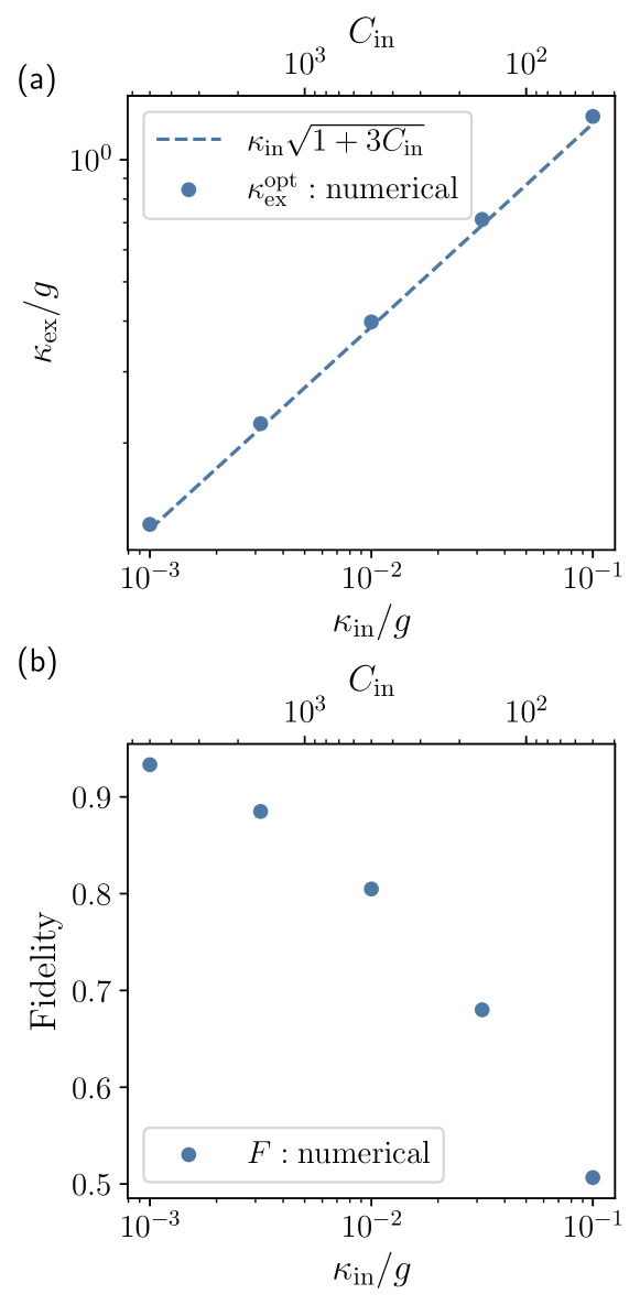
Figure 5: Optimized $\kappa_{\text{ex}}$ for generating the four-component cat state. The parameters other than $\kappa_{\text{in}}$ are the same as Fig. 2 and we set $\tau=5\tau_{c}$. (a) Numerically optimized $\kappa_{\text{ex}}$ to maximize the fidelity $F$. (b) Numerical results for $F$ with numerically optimized $\kappa_{\text{ex}}$.

IV Conclusion

We have proposed a protocol to generate propagating cat states by driving 4LSs inside a cavity. Using a single 4LS, we can deterministically generate the Schrödinger-cat entangled states, which have applications in quantum communication [37, 38]. Moreover, using two 4LSs, we can generate a four-component cat state after postselecting the state of the two 4LSs. The Schrödinger-cat entangled state has already been generated with cavity QED, using the reflection scheme proposed by Wang and Duan [17, 16]. In principle, a four-component cat can also be generated by repeated use of the reflection scheme and postselection twice. In this case, however, the propagating two-component cat state must pass through a circulator and be reflected by a cavity with finite loss, which was 19% in the previous work [17]. Thus, generating a four-component cat state with the reflection method may not be feasible. Our protocol can generate it without circulators and multiple reflections, and hence it will be a more promising method to generate complex CV states. Our method will require $C_{\text{in}}>10^{3}$ to generate desired states with fidelity close to unity. Albeit such high internal cooperativity may be challenging, cavity designs that achieve the internal cooperativity exceeding $10^{3}$ have been proposed and even realized experimentally [39, 40, 41], making our method feasible in the near future.

Finally, we note that adding more 4LSs can generate more complex CV states. In general, our protocol can generate the entanglement between $N$ 4LSs and a superposition of $2^{N}$ coherent states: $\sum_{\{j^{(i)}\}}b_{j^{(1)}j^{(2)}\cdots j^{(N)}}\ket*{j^{(1)}j^{(2)}\cdots j^{(N)}}\ket*{\sum_{i}(-1)^{j^{(i)}}\alpha_{i};v}$ (see Appendix B). Thus, combining linear optics or squeezers with our protocol would provide a method to generate more complex and more useful CV states with high fidelity.

Appendix A Derivation of the effective master equation

We rewrite the Hamiltonian of a single 4LS in a proper rotating frame in Eq. (1) as

$$\hat{H}_{\text{4LS}}= \hat{H}_{e}+\hat{V}(t)+\hat{V}^{\dagger}(t),$$ (18)

$$\hat{H}_{e}= \ab(\Delta-\frac{\delta_{e}}{2})\outerproduct{e_{1}}{e_{1}}+\ab(\Delta+\frac{\delta_{e}}{2}-\delta_{g})\outerproduct{e_{2}}{e_{2}},$$

$$\hat{V}(t)= \Omega(t)(\outerproduct{e_{2}}{\downarrow}+\outerproduct{e_{1}}{\uparrow})+g(\outerproduct{e_{1}}{\downarrow}+\outerproduct{e_{2}}{\uparrow})\hat{c}.$$

Here, assuming the case where excited states $\{\ket{e_{1}},\ket{e_{2}}\}$ quickly reach steady states, we can adiabatically eliminate excited states. Such adiabatical elimination can be systemically done by using an effective operator formalism with time-dependent couplings as follows [43, 44]. First, we define a non-Hermitian Hamiltonian as

$$\hat{H}_{\text{NH}}= \hat{H}_{e}-\frac{i}{2}\sum_{m=2}^{5}\hat{L}_{m}^{\dagger}\hat{L}_{m}$$ (19)

$$= \ab(\Delta-\frac{\delta_{e}}{2}-i\gamma)\outerproduct{e_{1}}{e_{1}}+\ab(\Delta+\frac{\delta_{e}}{2}-\delta_{g}-i\gamma)\outerproduct{e_{2}}{e_{2}},$$

where $\hat{L}_{m}$ is defined in Eq. (8). By using this operator, the effective operators are given as follows:

$$\hat{H}^{\text{eff}}_{\text{4LS}}(t)= -\frac{1}{2}\hat{V}^{\dagger}(t)[\hat{H}_{\text{NH}}^{-1}+(\hat{H}_{\text{NH}}^{-1})^{\dagger}]\hat{V}(t),$$ (20)

$$\hat{L}_{m}^{\text{eff}}(t)= \hat{L}_{m}\hat{H}_{\text{NH}}^{-1}\hat{V}(t)\quad(m=2,3,\cdots,5),$$

where

$$\hat{H}_{\text{NH}}^{-1}=\ab(\Delta-\frac{\delta_{e}}{2}-i\gamma)^{-1}\outerproduct{e_{1}}{e_{1}}+\ab(\Delta+\frac{\delta_{e}}{2}-\delta_{g}-i\gamma)^{-1}\outerproduct{e_{2}}{e_{2}}.$$ (21)

Substituting Eqs. (18) and (19) into Eq. (20) gives

$$\hat{H}^{\text{eff}}_{\text{4LS}}= -\real\ab[\frac{1}{\Delta-\delta_{e}/2-i\gamma}]\ab[|\Omega|^{2}\outerproduct{\uparrow}{\uparrow}+g^{2}\outerproduct{\downarrow}{\downarrow}\hat{c}^{\dagger}\hat{c}+(\Omega g\hat{\sigma}_{-}\hat{c}^{\dagger}+\text{H.c.})]$$ (22)

$$-\real\ab[\frac{1}{\Delta+\delta_{e}/2-\delta_{g}-i\gamma}]\ab[|\Omega|^{2}\outerproduct{\downarrow}{\downarrow}+g^{2}\outerproduct{\uparrow}{\uparrow}\hat{c}^{\dagger}\hat{c}+(\Omega g\hat{\sigma}_{+}\hat{c}^{\dagger}+\text{H.c.})],$$

$$\hat{L}_{2}^{\text{eff}}= \frac{\sqrt{2r_{1}\gamma}}{\Delta-\delta_{e}/2-i\gamma}(\Omega\hat{\sigma}_{-}+g\outerproduct{\downarrow}{\downarrow}\hat{c}),$$

$$\hat{L}_{3}^{\text{eff}}= \frac{\sqrt{2(1-r_{1})\gamma}}{\Delta-\delta_{e}/2-i\gamma}(\Omega\outerproduct{\uparrow}{\uparrow}+g\hat{\sigma}_{+}\hat{c}),$$

$$\hat{L}_{4}^{\text{eff}}= \frac{\sqrt{2r_{2}\gamma}}{\Delta+\delta_{e}/2-\delta_{g}-i\gamma}(\Omega\hat{\sigma}_{+}+g\outerproduct{\uparrow}{\uparrow}\hat{c}),$$

$$\hat{L}_{5}^{\text{eff}}= \frac{\sqrt{2(1-r_{2})\gamma}}{\Delta+\delta_{e}/2-\delta_{g}-i\gamma}(\Omega\outerproduct{\downarrow}{\downarrow}+g\hat{\sigma}_{-}\hat{c}).$$

Here, we assume $|\Delta|\gg\delta_{g},\delta_{e},\gamma$ and then the effective operators can be approximated as

$$\hat{H}^{\text{eff}}_{\text{4LS}}= -\frac{g^{2}}{\Delta}\hat{c}^{\dagger}\hat{c}-\frac{g}{\Delta}\hat{\sigma}_{x}(\Omega^{\ast}(t)\hat{c}+\Omega(t)\hat{c}^{\dagger})=\omega_{0}\hat{c}^{\dagger}\hat{c}+\hat{\sigma}_{x}(\lambda^{\ast}(t)\hat{c}+\lambda(t)\hat{c}^{\dagger}),$$ (23)

$$\hat{L}_{2}^{\text{eff}}= \frac{\sqrt{2r_{1}\gamma}}{\Delta}(\Omega\hat{\sigma}_{-}+g\outerproduct{\downarrow}{\downarrow}\hat{c})=-\frac{\sqrt{2r_{1}\gamma}}{g}(\lambda(t)\hat{\sigma}_{-}+\omega_{0}\outerproduct{\downarrow}{\downarrow}\hat{c}),$$

$$\hat{L}_{3}^{\text{eff}}= \frac{\sqrt{2(1-r_{1})\gamma}}{\Delta}(\Omega\outerproduct{\uparrow}{\uparrow}+g\hat{\sigma}_{+}\hat{c})=-\frac{\sqrt{2(1-r_{1})\gamma}}{g}(\lambda(t)\outerproduct{\uparrow}{\uparrow}+\omega_{0}\hat{\sigma}_{+}\hat{c}),$$

$$\hat{L}_{4}^{\text{eff}}= \frac{\sqrt{2r_{2}\gamma}}{\Delta}(\Omega\hat{\sigma}_{+}+g\outerproduct{\uparrow}{\uparrow}\hat{c})=-\frac{\sqrt{2r_{2}\gamma}}{g}(\lambda(t)\hat{\sigma}_{+}+\omega_{0}\outerproduct{\uparrow}{\uparrow}\hat{c}),$$

$$\hat{L}_{5}^{\text{eff}}= \frac{\sqrt{2(1-r_{2})\gamma}}{\Delta}(\Omega\outerproduct{\downarrow}{\downarrow}+g\hat{\sigma}_{-}\hat{c})=-\frac{\sqrt{2(1-r_{2})\gamma}}{g}(\lambda(t)\outerproduct{\downarrow}{\downarrow}+\omega_{0}\hat{\sigma}_{-}\hat{c}),$$

where we have neglected the term of the identity operator in the Hamiltonian and defined

$$\omega_{0}=-\frac{g^{2}}{\Delta},\quad\lambda(t)=-\frac{g\Omega(t)}{\Delta}.$$ (24)

Similarly, the effective Hamiltonian of $N$ 4LSs is approximately given by

$$\hat{H}^{\text{eff}}_{\text{4LSs}}= \sum_{i=1}^{N}\hat{H}_{\text{4LS},i}^{\text{eff}},$$ (25)

$$\hat{H}_{\text{4LS},i}^{\text{eff}}= \omega_{0}\hat{c}^{\dagger}\hat{c}+\hat{\sigma}_{x,i}(\lambda^{\ast}_{i}(t)\hat{c}+\lambda_{i}(t)\hat{c}^{\dagger}),$$

where we define $\hat{\sigma}_{x,i}=\outerproduct{\uparrow}{\uparrow}[_{i}]{\downarrow}+\outerproduct{\downarrow}{\downarrow}[_{i}]{\uparrow}$ and $\lambda_{i}(t)=-g\Omega_{i}(t)/\Delta$. To simulate the output field from the cavity based on the virtual-cavity method [25, 26], we numerically solve the following effective master equation:

$$\odv{\hat{\rho}}{t}= -i[\hat{H}^{\text{eff}},\hat{\rho}]+\sum_{m=0,1}\ab(\hat{L}_{m}\hat{\rho}\hat{L}_{m}^{\dagger}-\frac{1}{2}\{\hat{L}_{m}^{\dagger}\hat{L}_{m},\hat{\rho}\})+\sum_{i=1}^{N}\sum_{m\geq 2}\ab(\hat{L}_{m}^{i,\text{eff}}\hat{\rho}(\hat{L}_{m}^{i,\text{eff}})^{\dagger}-\frac{1}{2}\{(\hat{L}_{m}^{i,\text{eff}})^{\dagger}\hat{L}_{m}^{i,\text{eff}},\hat{\rho}\}),$$ (26)

where

$$\begin{gathered}\hat{H}^{\text{eff}}=\hat{H}^{\text{eff}}_{\text{4LSs}}+\frac{i}{2}\sqrt{2\kappa_{\text{ex}}}\ab[g_{v}^{\ast}(t)\hat{c}^{\dagger}\hat{a}_{v}-g_{v}(t)\hat{c}\hat{a}_{v}^{\dagger}],\\ \hat{L}_{0}(t)=\sqrt{2\kappa_{\text{ex}}}\hat{c}+g_{v}^{\ast}(t)\hat{a}_{v}(t),\quad\hat{L}_{1}=\sqrt{2\kappa_{\text{in}}}\hat{c},\end{gathered}$$ (27)

and the effective Lindblad operators $\hat{L}_{m}^{i,\text{eff}}$ are given by replacing $(\hat{\sigma}_{\pm},\outerproduct{\uparrow}{\uparrow},\outerproduct{\downarrow}{\downarrow})$ with $(\hat{\sigma}_{\pm,i},\outerproduct{\uparrow}{\uparrow}[_{i}]{\downarrow},\outerproduct{\downarrow}{\downarrow}[_{i}]{\downarrow})$ in Eq. (23). To evaluate the unnormalized state with no quantum jumps $\ket{\Psi}$, we numerically solve the following effective non-Hermitian Schrödinger equation:

$$i\odv{\ket{\Psi}}{t}= \hat{\mathcal{H}}^{\text{eff}}\ket{\Psi},$$ (28)

$$\hat{\mathcal{H}}^{\text{eff}}= \hat{H}^{\text{eff}}-\frac{i}{2}\ab(\sum_{m=0,1}\hat{L}_{m}^{\dagger}\hat{L}_{m}+\sum_{i=1}^{N}\sum_{m\geq 2}(\hat{L}_{m}^{i,\text{eff}})^{\dagger}\hat{L}_{m}^{i,\text{eff}}).$$

Appendix B Input-output theory with multiple 4LSs inside a cavity

We consider the case with $N$ 4LSs inside a cavity. We assume that the 4LSs are initially in the spin manifold $\{\ket{\downarrow},\ket{\uparrow}\}$, and both of the cavity and output modes are in vacuum states. From the relation $[\hat{\sigma}_{x,i},\hat{H}_{\text{4LSs}}^{\text{eff}}]=0$, $\hat{\sigma}_{x,i}(t)$ is time-independent and can be denoted simply by $\hat{\sigma}_{x,i}(0)$. For $\hat{c}(t)$, we obtain

$$\dot{\hat{c}}=-(iN\omega_{0}+\kappa)\hat{c}-i\sum_{i}\lambda_{i}(t)\hat{\sigma}_{x_{i}}(0).$$ (29)

Here, we choose the laser field $\Omega_{i}(t)$ satisfying

$$\lambda_{i}(t)=\frac{i\alpha_{i}}{\sqrt{2\kappa_{\text{ex}}}}\ab[\dot{v}(t)+(iN\omega_{0}+\kappa)v(t)].$$ (30)

Substituting it into Eq. (29) gives

$$\hat{c}(t)=\frac{v(t)}{\sqrt{2\kappa_{\text{ex}}}}\sum_{i}\alpha_{i}\hat{\sigma}_{x,i}(0)$$ (31)

and we find that the output desired mode is given as $\hat{a}_{\text{out}}(t)=v(t)\sum_{i}\alpha_{i}\hat{\sigma}_{x,i}(0)$ by using the input-output relation $\hat{a}_{\text{out}}(t)=\sqrt{2\kappa_{\text{ex}}}\hat{c}(t)$. Thus, after driving 4LSs, the output desired mode becomes a coherent state with a temporal mode $v(t)$ whose amplitude depends on the initial state of $N$ 4LSs.

Appendix C Evaluating $F_{\text{min}}$ for the generation of the Schrödinger-cat entangled state

We show the derivation of $F_{\text{min}}$ in Eq. (14). The total Hamiltonian is given as follows:

$$\hat{H}_{\text{total}}(t)= \hat{H}^{\text{eff}}_{\text{4LS}}(t)+\hat{H}_{B}+\hat{H}_{\text{int}},$$ (32)

$$\hat{H}^{\text{eff}}_{\text{4LS}}(t)= \omega_{0}\hat{c}^{\dagger}\hat{c}+\hat{\sigma}_{x}(\lambda^{\ast}(t)\hat{c}+\lambda(t)\hat{c}^{\dagger}),$$

$$\hat{H}_{B}= \sum_{i=0,1}\int\differential{k}k\hat{a}_{i}^{\dagger}(k)\hat{a}_{i}(k),$$

$$\hat{H}_{\text{int}}= \sum_{i=0,1}i\sqrt{\frac{\kappa_{i}}{\pi}}\int\differential{k}(\hat{a}_{i}^{\dagger}(k)\hat{c}-\hat{a}_{i}(k)\hat{c}^{\dagger}),$$

where $\hat{a}_{0}\,(\hat{a}_{1})$ is an annihilation operator of the desired output mode (the loss mode), and we have defined $(\kappa_{0},\kappa_{1})=(\kappa_{\text{ex}},\kappa_{\text{in}})$ and set the speed of light as $c=1$. In this section, we assume that the time width of the temporal mode $v(t)$ is sufficiently long and therefore $\aab*{\hat{c}^{\dagger}\hat{c}}\simeq 0$, which reduces the effective Lindblad operators as follows:

$$\hat{L}_{2}^{\text{eff}}= -\frac{\sqrt{2r_{1}\gamma}}{g}\lambda(t)\hat{\sigma}_{-},\quad\hat{L}_{3}^{\text{eff}}=-\frac{\sqrt{2(1-r_{1})\gamma}}{g}\lambda(t)\outerproduct{\uparrow}{\uparrow},$$ (33)

$$\hat{L}_{4}^{\text{eff}}= -\frac{\sqrt{2r_{2}\gamma}}{g}\lambda(t)\hat{\sigma}_{+},\quad\hat{L}_{5}^{\text{eff}}=-\frac{\sqrt{2(1-r_{2})\gamma}}{g}\lambda(t)\outerproduct{\downarrow}{\downarrow}.$$

Here, we consider the dynamics under the condition of no quantum jumps, which is described by a non-Hermitian Schrödinger equation:

$$\begin{gathered}i\odv*{\ket{\psi}}{t}=\hat{\mathcal{H}}\ket{\psi},\\ \hat{\mathcal{H}}=\hat{\mathcal{H}}^{\text{eff}}+\hat{H}_{B}+\hat{H}_{\text{int}},\\ \hat{\mathcal{H}}^{\text{eff}}=\hat{H}^{\text{eff}}(t)-\frac{i}{2}\sum_{m=2}^{5}(\hat{L}_{m}^{\text{eff}})^{\dagger}\hat{L}_{m}^{\text{eff}}=\omega_{0}\hat{c}^{\dagger}\hat{c}+\hat{\sigma}_{x}(\lambda^{\ast}(t)\hat{c}+\lambda(t)\hat{c}^{\dagger})-i\gamma\ab|\frac{\lambda(t)}{g}|^{2}\hat{I}.\end{gathered}$$ (34)

To reduce the difficulty of solving the dynamics, we use a frame where the amplitude of the output coherent state is always zero [45]. We apply the transformation of the Schrödinger equation with the operator $\hat{O}(t)$ as follows:

$$i\odv*{\ket{\psi(t)}_{O}}{t}= \hat{\mathcal{H}}_{O}(t)\ket{\psi(t)}_{O},$$ (35)

$$\ket{\psi(t)}_{O}\coloneqq \hat{O}(t)^{-1}\ket{\psi(t)},$$

$$\hat{\mathcal{H}}_{O}(t)\coloneqq \hat{O}(t)^{-1}\hat{\mathcal{H}}\hat{O}(t)+i\ab(\odv{\hat{O}^{-1}(t)}{t})\hat{O}(t).$$

We choose $\hat{O}(t)$ as

$$\hat{O}(t)=\exp\ab(-\gamma\int_{0}^{t}\differential{t^{\prime}}\ab|\frac{\lambda(t^{\prime})}{g}|^{2})e^{\hat{\sigma}_{x}(\beta(t)\hat{c}^{\dagger}-\beta^{\ast}(t)\hat{c})}\prod_{i}\exp\ab[\hat{\sigma}_{x}\int\differential{k}(\zeta_{i}(k,t)\hat{a}_{i}^{\dagger}(k)-\zeta_{i}^{\ast}(k,t)\hat{a}_{i}(k))],$$ (36)

where we assume

$$\begin{gathered}-i\dot{\zeta}_{i}(k,t)+k\zeta_{i}(k,t)+i\sqrt{\frac{\kappa_{i}}{\pi}}\beta(t)=0,\\ \zeta_{i}(k,0)=0.\end{gathered}$$ (37)

Equation (37) leads to

$$\zeta_{i}(k,t)=\sqrt{\frac{\kappa_{i}}{\pi}}\int_{0}^{t}\differential{\tau}\beta(\tau)e^{-ik(t-\tau)},$$ (38)

$$\sqrt{\frac{\kappa_{i}}{\pi}}\int\differential{k}\zeta_{i}(k,t)=\kappa_{i}\beta(t),$$ (39)

and we thus obtain

$$\hat{\mathcal{H}}_{O}(t)= \hat{O}(t)^{-1}\hat{\mathcal{H}}\hat{O}(t)+i\ab(\odv{\hat{O}^{-1}(t)}{t})\hat{O}(t)$$ (40)

$$= \omega_{0}\hat{c}^{\dagger}\hat{c}+\hat{H}_{B}+\hat{H}_{\text{int}}+\ab(\hat{\sigma}_{x}\hat{c}^{\dagger}\ab\{\lambda(t)-i[\dot{\beta}(t)+(i\omega_{0}+\kappa)\beta(t)]\}+\text{H.c.}).$$

By setting $\lambda(t)$ as

$$\lambda(t)=i[\dot{\beta}(t)+(i\omega_{0}+\kappa)\beta(t)],$$ (41)

we obtain $\hat{\mathcal{H}}_{O}=\omega_{0}\hat{c}^{\dagger}\hat{c}+\hat{H}_{B}+\hat{H}_{\text{int}}$. In the following, we assume $\beta(0)=0$ such that $\hat{O}(0)=\hat{I}$. Assuming the initial state as $\ket{\psi(0)}=\sum_{j}b_{j}\ket{j}\ket{0}_{c}\ket{\text{vac}}$, where $\ket{\text{vac}}$ denotes a vacuum state of all output modes, we obtain

$$\ket{\psi(t)}_{O}=e^{-i\hat{\mathcal{H}}_{O}t}\ket{\psi(0)}=\sum_{j}b_{j}\ket{0}_{c}\ket{j}\ket{\text{vac}}.$$ (42)

Thus,

$$\ket{\psi(t)}= \hat{O}(t)\ket{\psi(t)}_{O}$$ (43)

$$= \exp\ab(-\gamma\int_{0}^{t}\differential{t^{\prime}}\ab|\frac{\lambda(t^{\prime})}{g}|^{2})e^{\hat{\sigma}_{x}(\beta(t)\hat{c}^{\dagger}-\beta^{\ast}(t)\hat{c})}\prod_{i}\exp\ab[\hat{\sigma}_{x}\int\differential{k}(\zeta_{i}(k,t)\hat{a}_{i}^{\dagger}(k)-\zeta_{i}^{\ast}(k,t)\hat{a}_{i}(k))]\ket{\psi(0)}.$$

Using Eq. (38) allows us to derive

$$\int\differential{k}\zeta_{i}(k,t)\hat{a}^{\dagger}_{i}(k)=\sqrt{2\kappa_{i}}\int_{0}^{t}\differential{\tau}\beta(\tau)\hat{a}_{i}^{\dagger}(z=t-\tau),$$ (44)

where we have defined

$$\hat{a}_{i}(z)=\frac{1}{\sqrt{2\pi}}\int\differential{k}e^{ikz}\hat{a}_{i}(k).$$ (45)

Here, we define $\beta(t)$ as $\sqrt{2\kappa_{\text{ex}}}\beta(t)=\alpha v(t)$ with $v(t)$ satisfying

$$\begin{gathered}\int_{0}^{\infty}\differential{t}|v(t)|^{2}=1,\\ v(0)=\lim_{t\to\infty}v(t)=0.\end{gathered}$$ (46)

In this case, the generated state at a sufficiently large $t=T$ such that $\int_{0}^{T}\differential{t}|v(t)|^{2}=1$ becomes

$$\ket{\psi(T)}= \exp\ab(-\gamma\int_{0}^{T}\differential{t}\ab|\frac{\lambda(t)}{g}|^{2})\prod_{i}\exp\ab\{\hat{\sigma}_{x}\ab[\ab(\sqrt{\frac{\kappa_{\text{in}}}{\kappa_{\text{ex}}}})^{i}\alpha\int_{0}^{T}\differential{t}v(t)\hat{a}_{i}^{\dagger}(z=T-t)-\text{H.c.}]\}\ket{\psi(0)}$$ (47)

$$= \exp\ab(-\gamma\int_{0}^{T}\differential{t}\ab|\frac{\lambda(t)}{g}|^{2})\sum_{j}b_{j}\ket{0}_{c}\ket{j}\ket{(-1)^{j}\alpha;v}_{\text{ex}}\ket{(-1)^{j}\sqrt{\frac{\kappa_{\text{in}}}{\kappa_{\text{ex}}}}\alpha;v}_{\text{in}},$$

and the coupling strength is given as

$$\lambda(t)=\frac{i\alpha}{\sqrt{2\kappa_{\text{ex}}}}\ab[\dot{v}(t)+(i\omega_{0}+\kappa)v(t)].$$ (48)

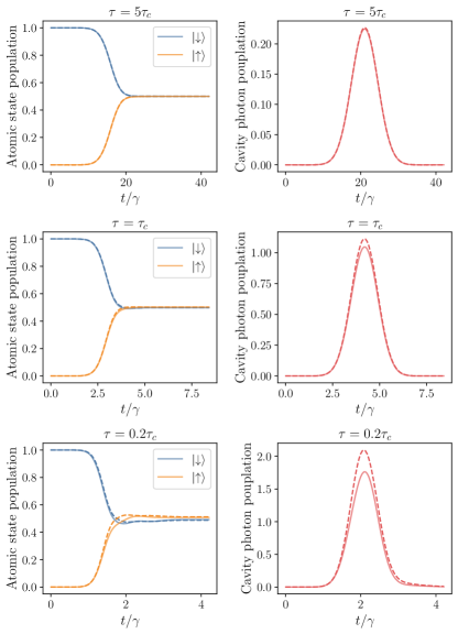
Figure 6: Comparison of the effective model with the full one in the case of the Schrödinger-cat entangled state generation with a 4LS inside a cavity. Solid lines represent the full model whereas dashed lines represent the effective model. The parameters are given as $(\Delta,g,\kappa_{\text{ex}},\kappa_{\text{in}})=(1000,10,1,0.01)\gamma$ and $r_{1}=r_{2}=0.5$.

Considering that we cannot access the mode that corresponds to the internal loss, we can decompose the generated state $\hat{\rho}=\outerproduct{\Psi}{\Psi}+\hat{\rho}_{\text{jumps}}$ with $\hat{\rho}_{\text{jumps}}$ representing an unnormalized state where one or more atomic decays or cavity losses occur and

$$\ket{\Psi}=\tensor{[}_{\text{in}}]{\innerproduct{0}{\psi(T)}}{}=\exp\ab(-\gamma\int_{0}^{T}\differential{t}\ab|\frac{\lambda(t)}{g}|^{2}-\frac{1}{2}\frac{\kappa_{\text{in}}}{\kappa_{\text{ex}}}|\alpha|^{2})\sum_{j}b_{j}\ket{0}_{c}\ket{j}\ket{(-1)^{j}\alpha;v}_{\text{ex}}$$ (49)

representing an unnormalized state where no atomic decay and cavity loss occur. Thus, the fidelity with the ideal state $\sum_{j}b_{j}\ket{j}\ket{0}_{c}\ket{(-1)^{j}\alpha;v}_{\text{ex}}$ is lower bounded as follows:

$$F\geq\exp\ab(-2\gamma\int_{0}^{T}\differential{t}\ab|\frac{\lambda(t)}{g}|^{2}-\frac{\kappa_{\text{in}}}{\kappa_{\text{ex}}}|\alpha|^{2})(\eqqcolon F_{\text{min}}).$$ (50)

Here, we assume a sufficiently large $\Delta$ such that $\omega_{0}/\kappa=-g^{2}/\kappa\Delta\simeq 0$. From Eq. (48),

$$\int_{0}^{T}\differential{t}|\lambda(t)|^{2}\simeq \frac{|\alpha|^{2}}{2\kappa_{\text{ex}}}\int_{0}^{T}\differential{t}\ab[|\dot{v}(t)|^{2}+\kappa\odv*{|v(t)|^{2}}{t}+\kappa^{2}|v(t)|^{2}]$$ (51)

$$= \frac{\kappa^{2}|\alpha|^{2}}{2\kappa_{\text{ex}}}\ab(1+\int_{0}^{T}\differential{t}\ab|\frac{\dot{v}(t)}{\kappa}|^{2}).$$

Assuming the long pulse such that $|\dot{v}(t)/\kappa|\simeq 0$ leads

$$F_{\text{min}}=\exp\ab[-\ab(\frac{\kappa}{\kappa_{\text{ex}}}\frac{1+2C}{2C}-1)|\alpha|^{2}],$$ (52)

where $C=g^{2}/2\kappa\gamma$ is the cooperativity.

Appendix D Validity of the effective model

We numerically simulate the dynamics of the full model for the Schrödinger-cat entangled state generation shown in Fig. 6. We find a discrepancy between the effective model and the full one for small $\tau/\tau_{c}$. As discussed in the main text, generating desired states with high fidelity requires $\tau\gg\tau_{c}$. Thus, our analysis based on the effective model should successfully predict the performance of state generation with high fidelity.

References

- Chen et al. [2014] M. Chen, N. C. Menicucci, and O. Pfister, Experimental realization of multipartite entanglement of 60 modes of a quantum optical frequency comb, Phys. Rev. Lett. 112, 120505 (2014).
- Larsen et al. [2019] M. V. Larsen, X. Guo, C. R. Breum, J. S. Neergaard-Nielsen, and U. L. Andersen, Deterministic generation of a two-dimensional cluster state, Science 366, 369 (2019).
- Asavanant et al. [2019] W. Asavanant, Y. Shiozawa, S. Yokoyama, B. Charoensombutamon, H. Emura, R. N. Alexander, S. Takeda, J. ichi Yoshikawa, N. C. Menicucci, H. Yonezawa, and A. Furusawa, Generation of time-domain-multiplexed two-dimensional cluster state, Science 366, 373 (2019).
- Kimble [2008] H. J. Kimble, The quantum internet, Nature 453, 1023 (2008).
- Mari and Eisert [2012] A. Mari and J. Eisert, Positive wigner functions render classical simulation of quantum computation efficient, Phys. Rev. Lett. 109, 230503 (2012).
- Hong and Mandel [1986] C. K. Hong and L. Mandel, Experimental realization of a localized one-photon state, Phys. Rev. Lett. 56, 58 (1986).
- Eaton et al. [2022] M. Eaton, C. González-Arciniegas, R. N. Alexander, N. C. Menicucci, and O. Pfister, Measurement-based generation and preservation of cat and grid states within a continuous-variable cluster state, Quantum 6, 769 (2022).
- McKeever et al. [2004] J. McKeever, A. Boca, A. D. Boozer, R. Miller, J. R. Buck, A. Kuzmich, and H. J. Kimble, Deterministic generation of single photons from one atom trapped in a cavity, Science 303, 1992 (2004).
- Morin et al. [2019] O. Morin, M. Körber, S. Langenfeld, and G. Rempe, Deterministic shaping and reshaping of single-photon temporal wave functions, Phys. Rev. Lett. 123, 133602 (2019).
- Keller et al. [2004] M. Keller, B. Lange, K. Hayasaka, W. Lange, and H. Walther, Continuous generation of single photons with controlled waveform in an ion-trap cavity system, Nature 431, 1075 (2004).
- Schupp et al. [2021] J. Schupp, V. Krcmarsky, V. Krutyanskiy, M. Meraner, T. Northup, and B. Lanyon, Interface between trapped-ion qubits and traveling photons with close-to-optimal efficiency, PRX Quantum 2, 020331 (2021).
- Sweeney et al. [2014] T. M. Sweeney, S. G. Carter, A. S. Bracker, M. Kim, C. S. Kim, L. Yang, P. M. Vora, P. G. Brereton, E. R. Cleveland, and D. Gammon, Cavity-stimulated raman emission from a single quantum dot spin, Nature Photonics 8, 442 (2014).
- Knall et al. [2022] E. N. Knall, C. M. Knaut, R. Bekenstein, D. R. Assumpcao, P. L. Stroganov, W. Gong, Y. Q. Huan, P.-J. Stas, B. Machielse, M. Chalupnik, D. Levonian, A. Suleymanzade, R. Riedinger, H. Park, M. Lončar, M. K. Bhaskar, and M. D. Lukin, Efficient source of shaped single photons based on an integrated diamond nanophotonic system, Phys. Rev. Lett. 129, 053603 (2022).
- Groiseau et al. [2021] C. Groiseau, A. E. J. Elliott, S. J. Masson, and S. Parkins, Proposal for a deterministic single-atom source of quasisuperradiant -photon pulses, Phys. Rev. Lett. 127, 033602 (2021).
- Gottesman et al. [2001] D. Gottesman, A. Kitaev, and J. Preskill, Encoding a qubit in an oscillator, Phys. Rev. A 64, 012310 (2001).
- Wang and Duan [2005] B. Wang and L.-M. Duan, Engineering superpositions of coherent states in coherent optical pulses through cavity-assisted interaction, Phys. Rev. A 72, 022320 (2005).
- Hacker et al. [2019] B. Hacker, S. Welte, S. Daiss, A. Shaukat, S. Ritter, L. Li, and G. Rempe, Deterministic creation of entangled atom–light schrödinger-cat states, Nature Photonics 13, 110–115 (2019).
- Hastrup and Andersen [2022a] J. Hastrup and U. L. Andersen, Protocol for generating optical gottesman-kitaev-preskill states with cavity qed, Phys. Rev. Lett. 128, 170503 (2022a).
- Vasilev et al. [2010] G. S. Vasilev, D. Ljunggren, and A. Kuhn, Single photons made-to-measure, New Journal of Physics 12, 063024 (2010).
- Utsugi et al. [2022] T. Utsugi, A. Goban, Y. Tokunaga, H. Goto, and T. Aoki, Gaussian-wave-packet model for single-photon generation based on cavity quantum electrodynamics under adiabatic and nonadiabatic conditions, Phys. Rev. A 106, 023712 (2022).
- Dimer et al. [2007] F. Dimer, B. Estienne, A. S. Parkins, and H. J. Carmichael, Proposed realization of the dicke-model quantum phase transition in an optical cavity qed system, Phys. Rev. A 75, 013804 (2007).
- Takahashi et al. [2017] H. Takahashi, P. Nevado, and M. Keller, Mølmer–sørensen entangling gate for cavity qed systems, Journal of Physics B: Atomic, Molecular and Optical Physics 50, 195501 (2017).
- Baden et al. [2014] M. P. Baden, K. J. Arnold, A. L. Grimsmo, S. Parkins, and M. D. Barrett, Realization of the dicke model using cavity-assisted raman transitions, Phys. Rev. Lett. 113, 020408 (2014).
- Gardiner and Collett [1985] C. W. Gardiner and M. J. Collett, Input and output in damped quantum systems: Quantum stochastic differential equations and the master equation, Phys. Rev. A 31, 3761 (1985).
- Kiilerich and Mølmer [2019] A. H. Kiilerich and K. Mølmer, Input-output theory with quantum pulses, Phys. Rev. Lett. 123, 123604 (2019).
- Kiilerich and Mølmer [2020] A. H. Kiilerich and K. Mølmer, Quantum interactions with pulses of radiation, Phys. Rev. A 102, 023717 (2020).
- Reiserer and Rempe [2015] A. Reiserer and G. Rempe, Cavity-based quantum networks with single atoms and optical photons, Rev. Mod. Phys. 87, 1379 (2015).
- Giannelli et al. [2018] L. Giannelli, T. Schmit, T. Calarco, C. P. Koch, S. Ritter, and G. Morigi, Optimal storage of a single photon by a single intra-cavity atom, New Journal of Physics 20, 105009 (2018).
- Goto et al. [2019] H. Goto, S. Mizukami, Y. Tokunaga, and T. Aoki, Figure of merit for single-photon generation based on cavity quantum electrodynamics, Phys. Rev. A 99, 053843 (2019).
- Grimsmo et al. [2020] A. L. Grimsmo, J. Combes, and B. Q. Baragiola, Quantum computing with rotation-symmetric bosonic codes, Phys. Rev. X 10, 011058 (2020).
- Su et al. [2022] D. Su, I. Dhand, and T. C. Ralph, Universal quantum computation with optical four-component cat qubits, Phys. Rev. A 106, 042614 (2022).
- Hastrup and Andersen [2022b] J. Hastrup and U. L. Andersen, All-optical cat-code quantum error correction, Phys. Rev. Res. 4, 043065 (2022b).
- Li and van Loock [2023] P.-Z. Li and P. van Loock, Memoryless quantum repeaters based on cavity-qed and coherent states, Advanced Quantum Technologies 6, 2200151 (2023).
- Hastrup et al. [2020] J. Hastrup, J. S. Neergaard-Nielsen, and U. L. Andersen, Deterministic generation of a four-component optical cat state, Opt. Lett. 45, 640 (2020).
- Thekkadath et al. [2020] G. S. Thekkadath, B. A. Bell, I. A. Walmsley, and A. I. Lvovsky, Engineering Schrödinger cat states with a photonic even-parity detector, Quantum 4, 239 (2020).
- Asavanant et al. [2021] W. Asavanant, K. Takase, K. Fukui, M. Endo, J.-i. Yoshikawa, and A. Furusawa, Wave-function engineering via conditional quantum teleportation with a non-gaussian entanglement resource, Phys. Rev. A 103, 043701 (2021).
- van Loock et al. [2006] P. van Loock, T. D. Ladd, K. Sanaka, F. Yamaguchi, K. Nemoto, W. J. Munro, and Y. Yamamoto, Hybrid quantum repeater using bright coherent light, Phys. Rev. Lett. 96, 240501 (2006).
- Azuma et al. [2012] K. Azuma, H. Takeda, M. Koashi, and N. Imoto, Quantum repeaters and computation by a single module: Remote nondestructive parity measurement, Phys. Rev. A 85, 062309 (2012).
- Hunger et al. [2010] D. Hunger, T. Steinmetz, Y. Colombe, C. Deutsch, T. W. Hänsch, and J. Reichel, A fiber fabry–perot cavity with high finesse, New Journal of Physics 12, 065038 (2010).
- Al-Sumaidae et al. [2018] S. Al-Sumaidae, M. H. Bitarafan, C. A. Potts, J. P. Davis, and R. G. DeCorby, Cooperativity enhancement in buckled-dome microcavities with omnidirectional claddings, Opt. Express 26, 11201 (2018).
- Ruddell et al. [2020] S. K. Ruddell, K. E. Webb, M. Takahata, S. Kato, and T. Aoki, Ultra-low-loss nanofiber fabry–perot cavities optimized for cavity quantum electrodynamics, Opt. Lett. 45, 4875 (2020).
- Krämer et al. [2018] S. Krämer, D. Plankensteiner, L. Ostermann, and H. Ritsch, Quantumoptics. jl: A julia framework for simulating open quantum systems, Computer Physics Communications 227, 109 (2018).
- Reiter and Sørensen [2012] F. Reiter and A. S. Sørensen, Effective operator formalism for open quantum systems, Phys. Rev. A 85, 032111 (2012).
- Kikura et al. [2024] S. Kikura, R. Asaoka, M. Koashi, and Y. Tokunaga, High-purity single-photon generation based on cavity qed (2024), arXiv:2403.00072 [quant-ph] .
- Goto and Koshino [2023] S. Goto and K. Koshino, Efficient numerical approach for the simulations of high-power dispersive readout with time-dependent unitary transformation, Phys. Rev. A 108, 033722 (2023).